From Prediction to Diagnostic Support: A Data-Driven System for Retail Demand Forecasting and Inventory Risk Assessment

Abstract

The rapid digital transformation of the retail industry has generated large-scale, high-frequency data; yet many retailers still rely on siloed systems that decouple demand forecasting from operational inventory management. This separation often leads to structural inventory imbalances, including simultaneous stockouts and overstock situations. To address this, we propose a unified, data-driven framework that integrates advanced sales forecasting with a diagnostic inventory health system, bridging predictive analytics with diagnostic decision support for proactive inventory-risk assessment. Utilizing a real-world dataset of approximately 500,000 product–store–day records from a Chinese e-commerce company, we evaluate six forecasting models across statistical, machine learning, and Deep Learning (DL) architectures. Results indicate that DL models achieved the lowest RMSE and MAPE values, whereas RF and XGBoost produced more favorable MASE values. Forecasting performance varied by evaluation criterion, with no model consistently outperforming all others. However, LSTM achieved the lowest testing RMSE (0.3996) and MAPE (21.63%). Building upon these predictive outputs, we introduce an inventory health diagnosis framework based on empirically calibrated thresholds for the Inventory Turnover Ratio (ITR) and Excess Inventory Rate (EIR), with the thresholds calibrated on the training and calibration period and evaluated on an independent temporal validation period. Application of this framework to the independent diagnostic validation period shows that 61.1% of SKU–store observations were classified as Potential Risk or Critical, including 16.3% classified as Critical, indicating inventory misalignment requiring managerial attention. By providing an interpretable and scalable system for proactive risk detection, this research provides a practical framework to support retailers in transitioning from demand forecasting to inventory diagnostic decision support.

1. Introduction

The rapid digital transformation of the retail industry has fundamentally reshaped global supply chains, shifting the focus from aggregate-level planning to high-frequency, granular decision-making. In the modern e-commerce landscape, retailers manage vast inventories across diverse geographical regions, generating millions of data points at the Stock Keeping Unit (SKU)–store level [1]. While this “Big Data” era offers unprecedented opportunities, the increasing complexity of these multi-dimensional environments makes accurate sales forecasting and effective inventory management essential for operational efficiency [1].

Despite advancements in predictive modelling, a persistent “operational silo” remains between demand forecasting and inventory management. Traditional systems often treat these as independent functions: data scientists optimize for mathematical accuracy, while operations managers struggle with physical challenges such as stockouts, overstocking, and aging stock [2]. This disconnect manifests as a structural imbalance where retail demand remains highly volatile due to internal factors, such as promotions, and external factors, such as seasonal events and regional characteristics [3,4].

Traditional forecasting approaches, such as Auto-Regressive Integrated Moving Average (ARIMA) or exponential smoothing, often fail to capture these nonlinear and irregular patterns [5]. Recent literature has increasingly applied DL to forecasting, including recurrent, attention-based, and specialized temporal architectures. LSTM remains widely used for modeling sequential dependencies, while Transformers capture interactions across historical observations [6,7]. Recent specialized architectures further highlight that model selection should consider accuracy, sequence length, data scale, heterogeneity, and computational requirements. However, a significant research gap remains: most studies analyze inventory metrics in isolation and fail to incorporate predicted demand directly into diagnostic processes [2,8]. Therefore, there is a critical need for a unified framework that translates forecasting outputs into interpretable diagnostic signals for proactive inventory risk detection.

This research addresses these challenges by proposing an integrated, data-driven system for retail sales forecasting and inventory health diagnosis. Utilizing a large-scale dataset of approximately 500,000 product–store–day records from Hengyuansheng (Quanzhou) Digital Technology Co., Ltd. (Quanzhou, China), we evaluate six models across three methodological families: statistical (Seasonal Naïve (SN) and Prophet), Machine Learning (ML) (Random Forest (RF) and Extreme Gradient Boosting (XGBoost)), and DL (LSTM and Transformer). Moving beyond simple error metrics, we introduce an original diagnostic framework based on event-calibrated thresholds for the Inventory Turnover Ratio (ITR) and Excess Inventory Rate (EIR).

The benchmark was designed as a representative cross-family comparison rather than an exhaustive evaluation. Seasonal Naïve and Prophet represent statistical methods, RF and XGBoost feature-based machine learning, and LSTM and Transformer recurrent and attention-based deep learning, respectively. This design balances diverse modeling assumptions with computational feasibility for the large-scale SKU–store dataset, while more specialized architectures were excluded to limit experimental scope.

To guide this investigation, we address the following three Research Questions (RQs):

RQ1: Which forecasting model provides the best performance for retail sales forecasting based on multiple evaluation metrics, including RMSE and MAPE?

RQ2: How can sales forecasting results be integrated to identify inventory health conditions effectively in a retail context?

RQ3: How can forecasting-based inventory analysis be made interpretable to support practical managerial decision-making?

The main contributions of this study are summarized as follows. First, we propose an integrated framework that combines demand forecasting with inventory health diagnostics to support managerial decision-making. Second, we deliver comprehensive benchmarking of forecasting models on a massive, real-world retail dataset. Third, we offer operational evidence of inventory health, revealing that over 60% of SKU–store combinations were classified as Potential Risk or Critical, indicating substantial inventory states requiring operational attention.

The main contribution of this work lies in integrating established forecasting methods with a data-driven inventory health diagnostic framework. Rather than proposing a novel forecasting algorithm, this study focuses on transforming forecasting outputs into interpretable diagnostic signals through an empirically calibrated thresholding mechanism that supports managerial decision-making.

The remainder of this paper is structured as follows: Section 2 reviews the related literature; Section 3 details the forecasting and diagnostic methodology; Section 4 presents the experimental results; and Section 5 discusses managerial implications and concludes the study.

2. Related Works

2.1. Evolution of Retail Demand Forecasting

Traditionally, retail demand forecasting relied on classical statistical models such as ARIMA and exponential smoothing. While these models are computationally efficient and offer high interpretability, they are primarily designed for stable, linear time-series data at aggregate levels [5]; however, their relative performance can vary substantially across retail datasets and demand characteristics, particularly when high-volatility and nonlinear patterns are present [9]. This has motivated increasing attention to ML and DL approaches for retail demand forecasting [9]. In the contemporary e-commerce context, SKU–store level sales data is frequently defined by “zero-inflation” (periods of no sales), and non-stationary patterns driven by external “shocks” such as promotions and holidays [1]. These complexities are compounded in retail environments where variable pricing strategies further influence daily consumption patterns, requiring models that can account for the non-linear relationship between price shifts and sales volume [10]. These complexities were notably highlighted in the M5 Accuracy Competition, which demonstrated that top-performing solutions for large-scale retail forecasting predominantly utilize ML and DL to handle such irregular data structures [11].

To address these complexities, the literature shifted toward adaptive frameworks like Prophet, which decomposes time series into trend, seasonality, and holiday effects. However, recent advancements have prioritized DL models to improve purchase forecasting accuracy, particularly in collaborative retail environments where producer-retailer teams must synchronize demand signals [12]. While Prophet improves upon ARIMA by handling irregular intervals and large seasonal shifts, it still struggles with the high-dimensional, nonlinear interactions present in multi-city retail environments [3,13]. Consequently, researchers have increasingly turned toward ML and DL to capture the “contextual features”, such as discount depth and regional characteristics, that dictate modern consumer behavior [4]; for instance, Ref. [14] demonstrated that combining clustering methods with ML can significantly improve prediction accuracy in specialized retail sectors by grouping similar historical sales patterns.

Recent time-series forecasting extends beyond conventional recurrent and Transformer models, incorporating specialized mechanisms such as temporal attention, multi-scale learning, variable selection, and probabilistic forecasting. Their suitability depends on factors including forecast horizon, historical context, data heterogeneity, feature availability, and computational resources. Therefore, for the one-day-ahead SKU–store task with a 14-day window, this study benchmarks representative statistical, machine-learning, recurrent, and attention-based models rather than the full forecasting landscape.

2.2. ML vs. DL in Supply Chains

The emergence of ML introduced robust ensemble-based methods to retail forecasting, most notably RF and XGBoost. Beyond ensemble techniques, distance-based learning approaches such as k-Nearest Neighbors (KNN) have also been utilized to generate forecasts by identifying historical observations with similar demand patterns, specifically to capture localized and short-term sales behavior [15]. These simpler regression-based models provide a useful baseline for evaluating how effectively more complex architectures can capture localized consumption shifts in retail environments [16]. They also excel at handling tabular data and high-dimensional feature sets, such as the interaction between price elasticities and local store characteristics [4]. By utilizing gradient boosting and bagging techniques, these architectures effectively mitigate the risk of overfitting in noisy retail environments. Furthermore, recent research has demonstrated that systematically optimizing these ML models can significantly enhance their predictive stability across diverse retail categories [17]. However, a major limitation of standard ML models is their ‘memoryless’ nature; they typically treat each time step as an independent observation unless time-lagged features are manually engineered [3].

Recent research increasingly adopts DL models for sequential data, demonstrating strong retail forecasting performance by capturing temporal dependencies and nonlinear relationships with less reliance on engineered temporal features [18,19]. However, their advantage is dataset- and metric-dependent, and ML models remain competitive with informative tabular features, as also demonstrated by large-scale benchmarks such as the M5 competition [20]. Similar advantages have been observed in supermarket-specific studies, where daily product-level sequences were most accurately captured using neural architectures compared to traditional regression baselines [21]. Specifically, the development of architectures like the Temporal Fusion Transformer has advanced the field by enabling the seamless integration of static metadata and time-varying covariates while maintaining model interpretability [22]. Building on these architectural gains, recent frameworks have successfully embedded DL into comprehensive decision support systems, demonstrating that sophisticated temporal modeling can be directly translated into operational supply chain improvements [23]. LSTM networks, a variant of RNNs, have become the gold standard for multi-step forecasting due to their “gating” mechanisms, which allow the model to retain long-term dependencies while discarding irrelevant noise [6,24]. Recently, Transformer models, utilizing self-attention mechanisms, have demonstrated an ability to capture global dependencies across massive datasets [7]. More recently, empirical studies in the supermarket sector further validate that RNN-based architectures are highly effective at predicting the daily sales of individual products by learning from high-resolution transactional sequences [25]. While DL models offer superior accuracy, the literature highlights a trade-off: they are often viewed as “black boxes,” lacking the direct interpretability required for high-stakes managerial decisions. Addressing this, recent surveys highlight that modern research is increasingly focused on hybrid models and attention mechanisms that seek to balance high predictive performance with meaningful transparency [22]. Parallel advancements in specialized algorithms, such as the Exponential Factorization Machine, have further enhanced retail accuracy by explicitly modeling pairwise interactions between categorical SKU attributes while minimizing percentage error to better accommodate the high holding costs of perishable goods [26]. This study contributes to this debate by benchmarking these architectures specifically on their ability to translate high-frequency data into stable operational signals.

2.3. Inventory Management and Performance Metrics

Traditional inventory management literature has long focused on balancing service levels with holding costs. The ITR remains the most widely recognized metric for assessing operational efficiency, representing how many times a company’s inventory is sold and replaced over a specific period [8]; building on this, contemporary research in AI-driven operations highlights that such metrics are essential for enhancing inventory visibility and reducing manual errors in stock management [27]. While a high ITR generally indicates lean operations, it can be deceptive in isolation; it fails to distinguish between a healthy “high-velocity” SKU and one that is perpetually understocked, leading to lost sales and customer dissatisfaction [2,28].

To provide a more holistic view of “Inventory Health,” recent studies have introduced the EIR as a critical counterpart to turnover. EIR measures the proportion of stock that exceeds forecasted demand, directly quantifying the capital tied up in non-performing assets. Despite the individual utility of these metrics, a significant gap remains in the literature: most research treats ITR and EIR as “lagging indicators”, post-hoc measurements of what has already occurred. There is a lack of “proactive diagnostics” that integrate real-time, high-frequency sales forecasts into an automated health-state categorization (e.g., Healthy, Potential Risk, Critical), which is a gap that must be addressed as AI-based systems introduce automated methods for detecting inventory discrepancies and optimizing replenishment [27]. This study addresses this gap by utilizing event-calibrated thresholds, adjusting the “health” definition based on promotional peaks and seasonal troughs, to provide a more nuanced diagnostic signal than static industry benchmarks [2].

2.4. Synthesis and Research Gap

A synthesis of the current literature reveals two primary trends: (1) a rapid advancement in DL models for capturing complex, non-linear demand patterns, and (2) a well-established set of inventory metrics such as ITR and EIR. However, these two domains remain largely fragmented. Most research focuses on improving forecasting accuracy (minimizing RMSE or MAPE) without establishing a direct link to operational ‘health’ diagnostics [1]. Conversely, inventory studies often utilize historical data, lacking the “forward-looking” predictive power required for proactive risk management [2].

The research gap is most evident at the SKU–store level, where the sheer volume and noise of high-frequency e-commerce data often lead to “analysis paralysis” for human managers. There is a demonstrable need for an integrated framework that not only predicts demand with high precision but also translates those predictions into an interpretable, event-calibrated diagnostic system. By bridging the gap between predictive analytics and inventory diagnostic decision support, this study provides a scalable framework that enables retailers to proactively identify inventory health risks and support managerial decision-making [27].

In summary, while the literature has made significant strides in isolated areas of demand forecasting and inventory metrics, there remains a critical need for a unified diagnostic decision-support system that operates at the high-frequency SKU–store level. The existing fragmentation between predictive accuracy and operational health signals represents a significant barrier to proactive retail management. To address this gap, the following section details our proposed methodology, which integrates advanced DL forecasting with a novel, event-calibrated inventory diagnostic framework.

Table 1. Comparison of Retail Sales Forecasting Models and Reported Performance.

Ref.	Model	Dataset	MAPE%	RMSE
[1]	Prophet	UK Retail Sales Time Series	13.2	-
	XGBoost	UK Grocery Retail Data	8.9	-
	LightGBM		8.3	-
	RF		9.5	-
	Transformer	Retail Benchmark Dataset	6.1	-
[15]	KNN	Indian Retail Stores	11.6	0.898
[20]	LSTM	M5 Walmart Retail	7.8	0.289
[24]	GRU	Fashion and Apparel Retail Sales Dataset	6.7	-

and

Table 2. Comparison of Retail Sales Forecasting Models of Daily Dataset.

Ref.	Model	Dataset	RMSE%
[29]	ARIMA (1,1,1)	Walmart, single SKU	1.13
	Prophet		1.71
	LightGBM (Category Sample Avg.)	Walmart, 100 sampled SKUs	1.1883
[21]	Linear Regression	Brazil supermarket, same dataset	5–8
	LSTM (top 25% SKUs)	Brazil supermarket, l-performing SKUs	1.55
	GRU (top 25% SKUs)	Brazil supermarket, same subset	1.55–1.60
[26]	ATLAS(S)	Weekly sales forecasts for 8 product categories	5.54–78.91

synthesize selected existing works, comparing model performance across various reporting frequencies and benchmarking the predictive accuracy of DL models against traditional statistical methods.

3. Materials and Methods

The proposed framework is conceptualized as a dual-layer architecture comprising a Predictive Layer, optimized for high-frequency SKU–store sales forecasting, and an Inventory Health Diagnostic Layer, designed to identify inventory conditions and generate interpretable, rule-based managerial decision-support signals. This section details the multi-dimensional spatial-temporal characteristics of the utilized dataset, the diverse modeling families employed for temporal analysis, and the event-calibrated diagnostic logic developed to translate inventory states into decision-ready managerial signals. The diagnostic layer is intended to support managerial decision-making rather than to perform formal prescriptive inventory optimization.

3.1. Data Source and Preprocessing

The empirical basis of this research is a large-scale longitudinal dataset provided by HENGYUANSHENG (QUAN ZHOU) DIGITAL TECHNOLOGY, Quanzhou, Fuijan, China, a leading Chinese e-commerce enterprise. The raw data encompasses approximately 500,000 product–store–day records, spanning multiple product categories across diverse geographical regions ranging from Tier-1 to Tier-3 cities. The primary unit of analysis is the SKU–store level; this granular approach ensures that localized demand variances, which are frequently obscured by aggregate corporate-level data, are accurately captured and modeled.

The predictive capacity of the framework relies on a multi-dimensional feature set, categorized into temporal, promotional, and regional variables as detailed in

Table 3. Feature List for Multi-Dimensional Demand Forecasting.

Feature	Description	Type
date	Date of each transaction	Temporal
city_name	Unique identifiers and names for cities participating in the dataset	Categorical
first_category, second_category, third_category	Product hierarchy from broad to fine-grained categories	Categorical
product	Unique identifier for individual products (SKUs)	Categorical
price	Price of each product	Numerical
sale_amount	Total sales amount for each product–store–date	Numerical
discount	Discount rate applied during the specific date	Numerical
Activity	Binary indicator (1 = promotional event, 0 = normal day)	Binary
stock_quantity	The exact on-hand inventory quantity is available at the store for the given product and date.	Numerical
Holiday	Binary indicator for public holidays or major sale days	Binary

. These variables allow the models to account for both baseline demand and external shocks, such as localized promotions and regional economic tiers.

To ensure the robustness of the forecasting models, a multi-stage preprocessing pipeline was implemented. The progression from data collection to the final diagnostic output is visually summarized in Figure 1. This research framework illustrates the sequential flow of the study: beginning with data acquisition and rigorous preprocessing, moving through the parallel development of the six forecasting models, and concluding with the multi-dimensional evaluation and inventory health diagnostic layers. By following this structured pipeline, the methodology ensures that high-frequency SKU–store data is converted into actionable managerial insights with both scientific and operational validity.

3.1.1. Dataset Quality Assessment

A data quality assessment was conducted after preprocessing to evaluate the completeness, consistency, and reliability of the dataset. The original dataset consisted of 500,000 product–store–day records collected from multiple product categories and geographical regions. Data cleaning procedures included missing value treatment, duplicate checking, categorical attribute imputation, and anomaly screening.

As summarized in

Table 4. Dataset Statistics Before and After Preprocessing.

Metric	Before Preprocessing	After Preprocessing
Records	500,000	459,310
Missing Values	27,555	0
Duplicate Records	0	0
Outliers	N/A	40,690
Zero-demand Ratio (%)	5.7	6.2

, 27,555 missing values were treated during preprocessing, with no duplicate records detected. Anomaly screening used a two-stage SKU–store-level procedure. First, observations below Q1 − 1.5 × IQR or above Q3 + 1.5 × IQR, where Q1 and Q3 are the first and third quartiles of each SKU–store sales distribution, were flagged only as candidate anomalies. Second, flagged observations were evaluated against recorded promotional, holiday, discount, inventory, and other operational events. Those with plausible event-related explanations were retained, while only unexplained statistical outliers were removed. Valid zero-demand observations were also retained.

Using this combined statistical and business-rule screening procedure, 40,690 potential anomalies were identified for removal. After preprocessing, the final dataset contained 459,310 records, representing 91.86% of the original observations. The processed dataset included 784 unique products (SKUs) and 558 stores, providing broad coverage for large-scale retail demand forecasting and inventory risk assessment. Missing values were imputed rather than removed; therefore, the reduction in record count was attributed to the anomaly-screening procedure.

Post-processing analysis showed that 6.2% of observations corresponded to zero-demand events, compared with 5.7% in the original dataset, indicating the presence of intermittent demand patterns. The final processed dataset was subsequently used for model training and evaluation.

To improve the transparency and reproducibility of the experimental setup, a summary of the dataset characteristics and forecasting configuration is provided in

Table 5. Dataset Summary and Forecasting Configuration.

Item	Value
Processed Records	459,310
Number of SKUs	784
Number of Stores	558
Number of Cities	136
Target Variable	Daily Sale Amount
Forecast Horizon	1 Day
Forecast Type	One-Step-Ahead Forecasting
Historical Window (Short-Term Context)	14 Days
Zero-Demand Ratio	6.2%
Train-Test Split	80%/20%
Data Partitioning	Chronological Split
Data Period	January 2022–December 2024

.

3.1.2. Exploratory Data Analysis (EDA)

Prior to algorithmic modeling, an EDA was performed to characterize the underlying statistical properties and demand dynamics within the Hengyuansheng ecosystem. This diagnostic phase focuses on identifying structural complexities, such as price elasticity, geographic variance, and category-specific seasonality, that the subsequent forecasting layer must accommodate.

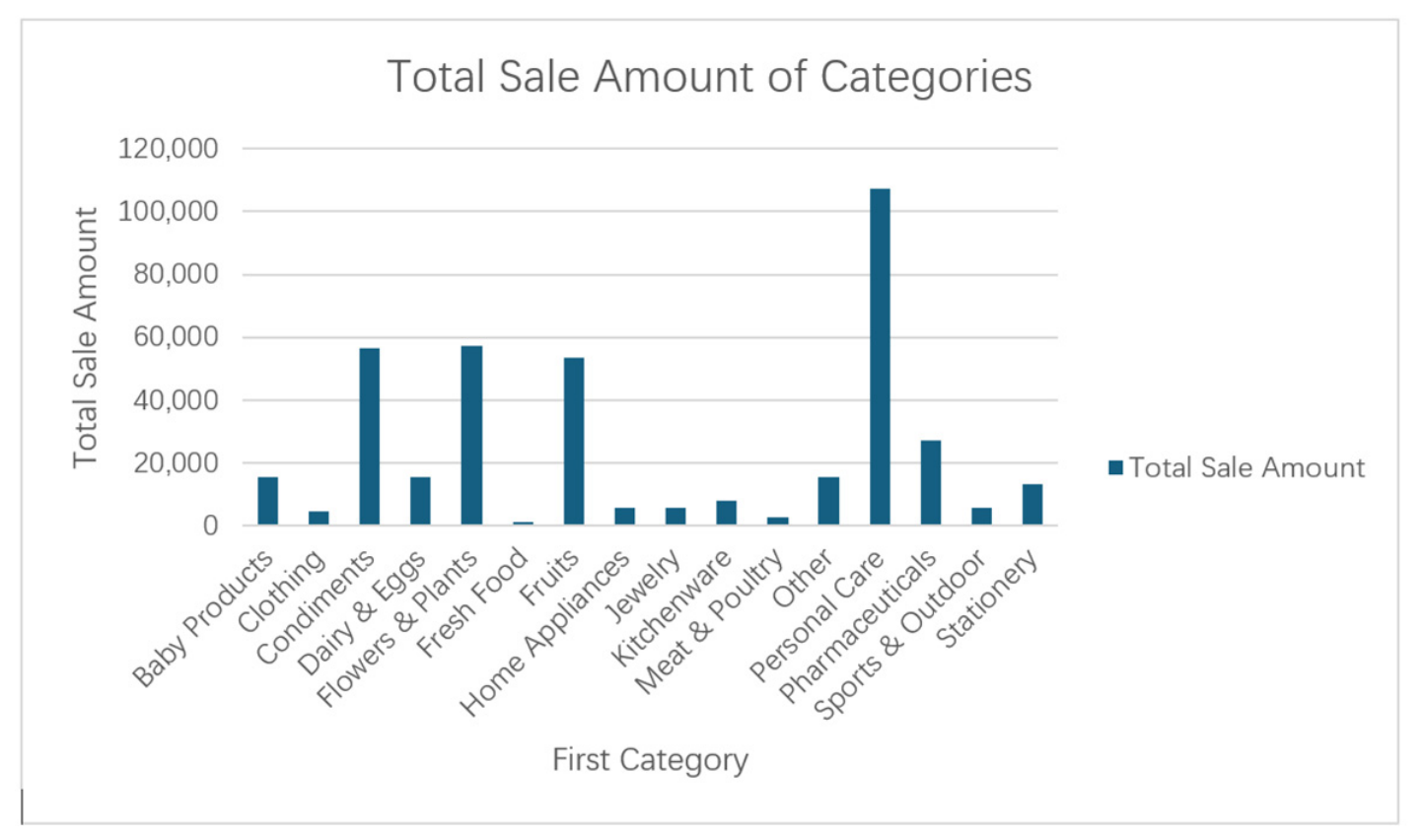
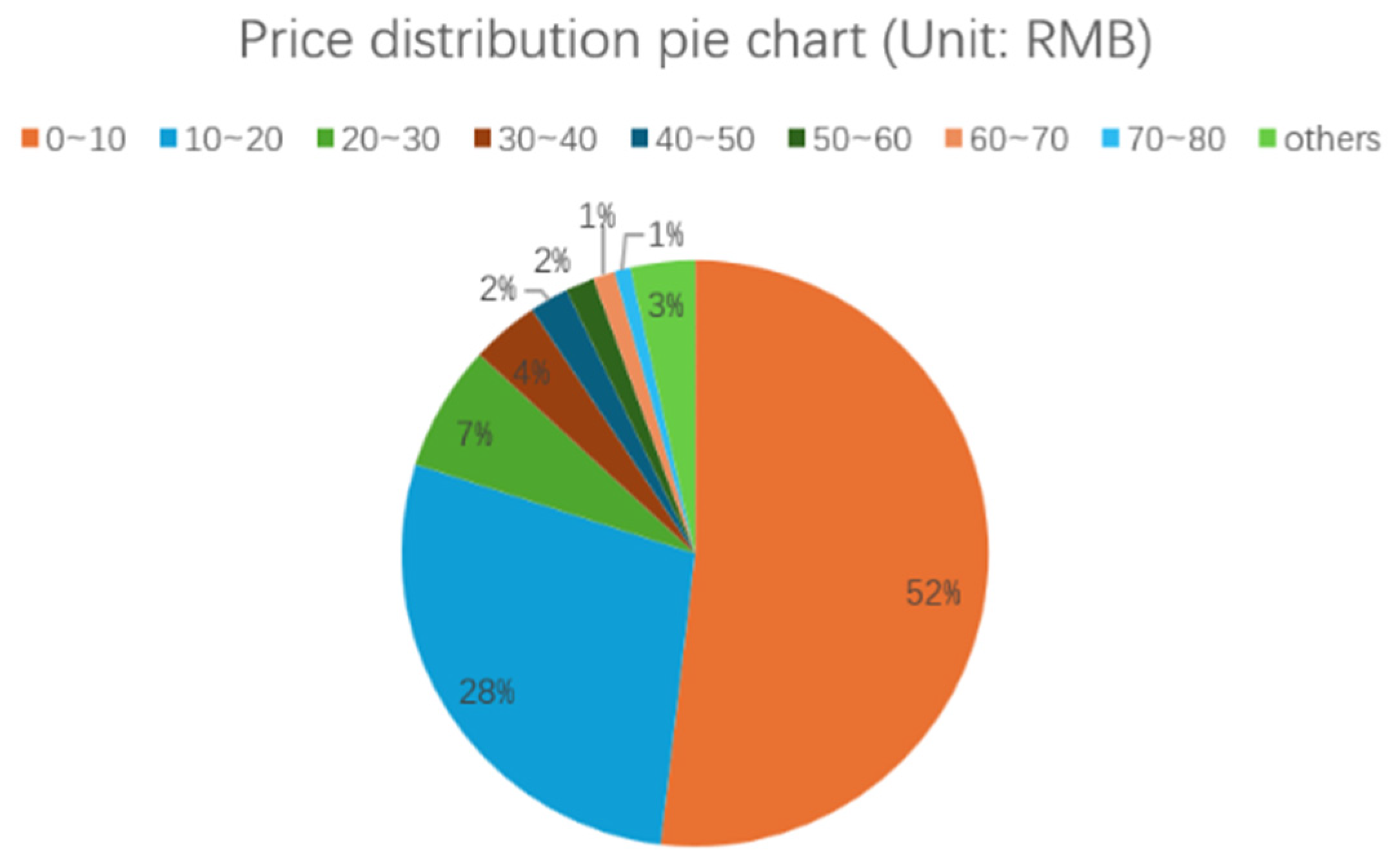
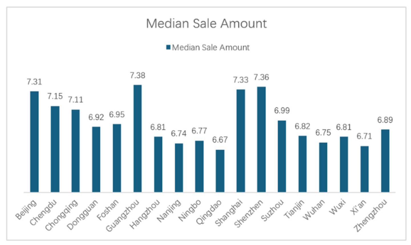
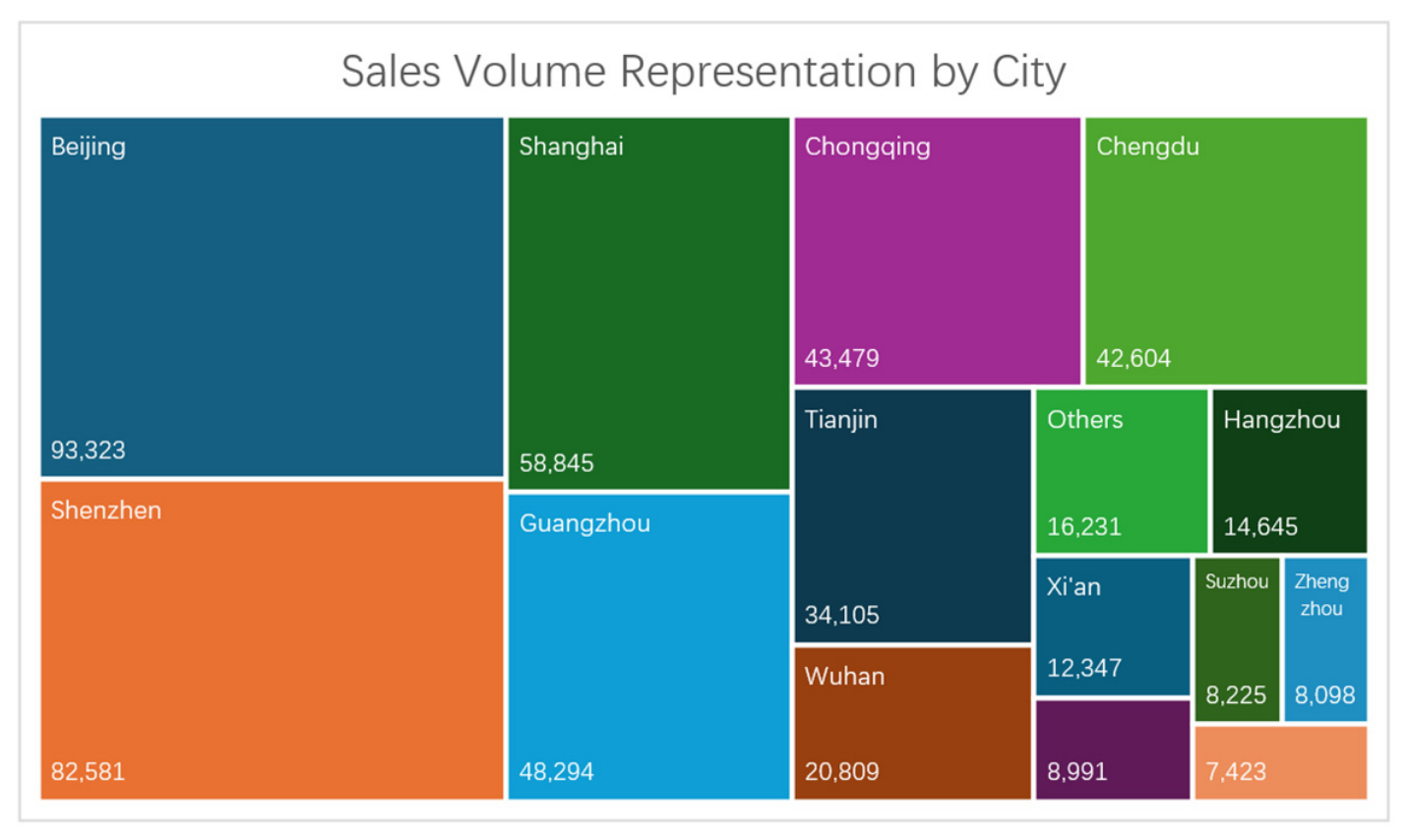
The economic diversity of the product portfolio is visualized in Figure 2, illustrating the varying price points that dictate consumer demand elasticity. The spatial complexity of the dataset is further elucidated through regional performance metrics; Figure 3 identifies distinct disparities in purchasing power across urban centers, while Figure 4 demonstrates that sales volume is non-uniformly distributed across product hierarchies. Finally, Figure 5 provides a geographic visualization of demand density. Collectively, these findings validate the inclusion of “City Tier” and “Category” as primary contextual features, as they represent the fundamental drivers of variance in SKU–store level sales.

3.1.3. Data Cleaning

To ensure the veracity of inputs for the algorithmic layer, the raw data underwent a rigorous cleaning and validation process. The primary challenge addressed was the zero-inflated nature of the SKU–store sales records; in high-frequency retail data, a value of ‘0’ typically denotes a lack of transactions (a “true zero”) rather than a recording error. Consequently, missing values were resolved using a combination of forward- and backward-filling techniques to maintain the continuity of temporal sequences without introducing synthetic bias. For missing categorical attributes, such as product hierarchy identifiers, values were imputed using mode imputation within each city-category cohort, a technique validated for preserving statistical integrity in high-frequency time-series databases [30].

Furthermore, an outlier screening procedure was applied at the SKU–store level using a two-stage statistical and business-context rule. An observation was first flagged as a candidate anomaly when its sales amount was below Q1 − 1.5 × IQR or above Q3 + 1.5 × IQR for its corresponding SKU–store series. The statistical flag was not used as an automatic exclusion criterion. Instead, flagged observations were cross-checked against the business-event variables available in the dataset, including promotional activity, holiday indicators, discount information, and inventory-related conditions. Observations associated with an identifiable business or operational event that could plausibly explain the extreme sales value were retained. Only observations that satisfied the IQR outlier criterion while lacking a corresponding recorded business or operational explanation were removed. This procedure was designed to reduce the influence of likely data-quality anomalies while preserving genuine demand shocks that may contain predictive information. Valid zero-demand observations were retained because they represent intermittent-demand behavior rather than missing or erroneous records.

3.1.4. Feature Engineering

To move beyond raw historical sales, the dataset was enriched with multi-dimensional contextual features designed to parameterize the operational environment of each SKU–store node. This process, summarized in Table 3, involved the extraction and encoding of features that capture exogenous demand drivers. First, temporal features were decomposed from transaction dates to account for cyclical fluctuations, such as day-of-the-week effects and weekends. Second, promotional and calendar indicators were integrated as binary flags to denote discount events and major public holidays (e.g., Lunar New Year). Forward- and backward-fill operations were applied only to missing values in the dataset, whereas valid zero-demand observations were preserved unchanged to reflect actual sales occurrences. Observations with zero demand were excluded from MAPE calculations to avoid undefined percentage errors.

These indicators enable the models to distinguish normal demand patterns from sudden demand fluctuations identified during the exploratory analysis. Finally, regional tiering was encoded to allow the models to learn varying consumer behaviors across different city classifications. By embedding these contextual layers, the feature engineering phase ensures that the predictive layer can generalize effectively across diverse product categories and geographic markets. All engineered features were generated using information available at or before the prediction time, thereby avoiding the use of future information during model development.

3.1.5. Data Transformation and Normalization

To ensure stability and convergence across the diverse modeling families, a rigorous transformation pipeline was applied to the engineered feature set. Given the significant variance in sales volumes and price points identified in Figure 2 and Figure 4, numerical features were normalized to a common scale ([0, 1]) [3]. This process is essential for preventing gradient explosion in the LSTM and Transformer architectures, where high-magnitude inputs can disproportionately influence weight updates. The normalization was carefully executed to ensure that the underlying temporal trends and relative variances, critical for capturing seasonal cycles, remained intact. Furthermore, categorical variables, such as City Tier and Product Category from Table 3, were transformed into numerical representations suitable for algorithmic processing. By aligning the disparate scales of price, quantity, and binary indicators, this transformation layer creates a mathematically cohesive input space for the subsequent predictive layer. The normalization parameters were estimated exclusively from the training data and then applied unchanged to the testing data to ensure a leakage-free evaluation.

3.1.6. Data Partitioning

To simulate real-world operational forecasting and prevent data leakage, the processed dataset was partitioned chronologically. Unlike random sampling, which can inadvertently allow models to “peek” into the future, a temporal split ensures that the evaluation reflects the model’s ability to generalize to unseen future sequences. As specified in the research design, an 80% training and calibration period was utilized to calibrate the parameters and weights of the six candidate models and to derive the inventory diagnostic thresholds. The remaining 20% served as an out-of-sample testing and independent diagnostic validation period, providing the “ground truth” for the forecasting performance metrics defined in Section 3.3.1 and for evaluating the inventory health diagnostic framework. This chronological separation ensures that the forecasting models and diagnostic thresholds are developed using only the earlier period, while their performance is evaluated on previously unseen observations. To further prevent data leakage, all preprocessing operations that required parameter estimation, including feature scaling and data transformation, were fitted using only the training and calibration dataset and subsequently applied to the test and validation dataset. Feature engineering was performed without utilizing future observations, ensuring that no information from the testing or diagnostic validation period was introduced into model training or threshold calibration.

3.2. Predictive Layer: Forecasting Models

3.2.1. Statistical Forecasting Models

The first family of models serves as a foundational benchmark, utilizing classical statistical and decomposition techniques to characterize the fundamental components of the time series. By isolating trend and seasonal patterns, these models provide a reference point for determining the “marginal gain” in accuracy offered by more computationally intensive ML architectures. This category includes the SN approach for baseline periodicity and the Prophet model for additive decomposition [5]. In this study, the SN model establishes the benchmark for intrinsic forecastability; a Mean Absolute Scaled Error (MASE) of 1.00 is defined as the baseline “no-skill” threshold. Consequently, a MASE value below 1.00 indicates lower scaled absolute error than the Seasonal Naïve benchmark, whereas a value above 1.00 indicates that the model does not improve upon the benchmark according to this metric. This comparison is descriptive and should not be interpreted as evidence of statistical significance.

SN: The SN model was implemented as a secondary baseline to provide a benchmark for the minimum acceptable forecasting accuracy. Unlike the parameterized models, SN assumes that the forecast for time is equal to the observed value at time, where represents the seasonal period [5]. For the dataset was set to 7 days to account for the strong weekly cyclicality identified in the EDA. This model serves to quantify the ‘value-add’ of the more complex algorithmic architectures; any model failing to outperform the SN baseline would be considered operationally insufficient.

Prophet: Prophet was selected as the statistical baseline due to its ability to model trend, seasonality, and holiday effects [5]. The model was configured with weekly and daily seasonality and incorporated external regressors, including discount, holiday, and promotional activity variables. The final hyperparameter configuration is presented in

Table 6. Hyperparameter Configuration and Seasonal Settings for the Prophet Baseline Model.

Parameter	Value	Description
Growth	Linear	Trend growth
Seasonality	Daily, Weekly	Enabled
Seasonality	Yearly	Disabled
Regressors	External regressors	Discount, Holiday, Activity
Training	Test window	28 days

.

3.2.2. ML Models

To capture the non-linear interactions between promotional activities, regional tiers, and historical sales, two ensemble learning architectures were implemented. These models move beyond the additive logic of the statistical baselines by utilizing decision-tree structures to partition the feature space into high-accuracy demand clusters.

RF: RF was selected as a representative ensemble ML model due to its strong performance in retail demand forecasting and its ability to capture nonlinear relationships among pricing, promotional, inventory, and regional variables [4]. Unlike statistical forecasting models that primarily rely on temporal patterns, RF can effectively utilize heterogeneous tabular features and is widely adopted as a benchmark model in retail forecasting studies [17]. Therefore, RF was included to evaluate the predictive capability of tree-based ensemble learning methods on high-frequency SKU–store demand data. The final hyperparameter configuration is presented in

Table 7. Hyperparameter Configuration for RF Model.

Parameter	Value	Description
n_estimators	600	Number of trees
max_depth	10	Maximum tree depth
min_samples_leaf	2	Minimum samples per leaf
min_samples_split	4	Minimum samples to split
n_jobs	−1	Parallel processing

.

XGBoost: XGBoost was included due to its proven effectiveness in retail demand forecasting and its ability to model complex feature interactions through gradient boosting [4]. The final hyperparameter settings are reported in

Table 8. Hyperparameter Configuration for XGBoost Model.

Parameter	Value	Description
max_depth	4	Max depth of trees
learning rate (eta)	0.01	Shrinkage rate
subsample	0.8	Row subsampling
colsample_bytree	0.8	Feature subsampling
objective	reg:squarederror	Regression loss
num_boost_round	2000	Max boosting rounds
early_stopping_rounds	20	Early stopping
eval_metric	RMSE	Evaluation metric

.

3.2.3. DL Models

To address the challenges of high-frequency sequences and short-term temporal dependencies in the dataset, two DL models were implemented: LSTM and Transformer. Both models used a 14-day historical input window to perform one-step-ahead forecasting. The 14-day window captures weekly seasonality, short-term demand persistence, and recent promotional effects while maintaining a manageable sequence length; thus, it represents short-term forecasting rather than long-term annual or multi-month dependencies.

LSTM: The LSTM network was selected due to its ability to model temporal dependencies within sequential demand data [6]. In the present study, the 14-day input window allows the model to capture recent demand persistence, weekly seasonality, and short-term promotional effects. This characteristic is particularly important for the present dataset, which exhibits seasonal fluctuations and promotion-driven demand shocks identified during the EDA stage. Previous studies have also demonstrated the effectiveness of LSTM in multi-category retail demand forecasting [6] and food-retailing applications involving complex supply–demand interactions [12]. The architectural configuration of the LSTM model is detailed in

Table 9. Hyperparameter Configuration for the LSTM Model.

Parameter	Value	Description
Window size	14	Short-term historical sequence length (days)
LSTM units	64	Hidden units in LSTM layer
Dense units	32	Fully connected layer size
Dropout	0.2	Dropout rate
Optimizer	Adam	Optimization algorithm
Batch size	32	Samples per batch
Epochs	30	Maximum epochs
Validation split	0.1	Validation ratio
Early stopping patience	6	Early stopping criterion

.

Transformer: Representing the frontier of sequence modeling, the Transformer architecture was implemented to leverage its self-attention mechanism. Unlike the sequential nature of LSTMs, Transformers process entire sequences in parallel, allowing the model to weigh the relative importance of different historical days regardless of their distance from the forecast date. Recent evidence suggests that Transformers can outperform traditional RNN-based approaches in capturing the long-range dependencies and sharp volatility found in SKU-level data [7]. Parameters of the Transformer are detailed in

Table 10. Hyperparameter Configuration for the Transformer Model.

Parameter	Value	Description
Window size	14	Short-term historical input sequence length (days)
d_model	32	Embedding dimension
Number of layers	2	Transformer encoder blocks
Number of heads	8	Multi-head self-attention
FF dimension	64	Hidden size in FFN
Dropout	0.2	Dropout rate
Optimizer	Adam	Gradient-based optimizer
Learning rate	0.001	Initial learning rate
Batch size	32	Samples per batch
Epochs	30	Maximum training epochs
Validation split	0.1	Fraction for validation
Early stopping patience	6	Early stopping criterion

.

3.2.4. Model Selection and Benchmarking Scope

The selected forecasting models were intended to provide methodological diversity rather than constitute an exhaustive benchmark of all contemporary time-series forecasting architectures. Seasonal Naive was used as a classical seasonal baseline, Prophet represented a widely adopted statistical forecasting approach, Random Forest and XGBoost represented nonlinear machine-learning methods, while LSTM and Transformer represented recurrent and attention-based deep-learning approaches, respectively. More specialized recent architectures, such as Temporal Fusion Transformer (TFT), PatchTST, and time-series foundation models, were not included in the current benchmark. Their inclusion would require additional model-specific preprocessing, hyperparameter tuning, and computational resources to ensure a fair comparison. Moreover, the present task focuses on one-day-ahead forecasting using a 14-day historical window, which provides a relatively short sequence compared with settings where long-range temporal modeling is central. Therefore, the current benchmark was designed to balance methodological diversity, computational feasibility, and comparability across model families. Nevertheless, benchmarking specialized contemporary forecasting architectures under the same experimental protocol remains an important direction for future research.

3.3. Inventory Health Diagnostic Layer

3.3.1. Metric Definitions

The health of an SKU–store combination is determined by the mathematical relationship between the forecasted demand, the actual inventory level (I), and the Cost of Goods Sold (COGS). Inventory health thresholds were calibrated using the training and calibration period and applied unchanged to the independent diagnostic validation period.

ITR: As calculated in (1) identifies the velocity of capital circulation. A declining ITR, when coupled with high forecasted demand, serves as an early warning for potential stockouts. In this study, ITR is defined as the ratio of average inventory level to COGS, derived from the actual cost of products sold in enterprise transaction records. Higher ITR indicates a larger inventory position relative to realized sales, slower circulation, and greater accumulation potential, while lower ITR indicates faster circulation.

$$\mathrm{I}\mathrm{T}\mathrm{R}={\displaystyle \frac{\mathrm{A}\mathrm{v}\mathrm{e}\mathrm{r}\mathrm{a}\mathrm{g}\mathrm{e} \mathrm{I}\mathrm{n}\mathrm{v}\mathrm{e}\mathrm{n}\mathrm{t}\mathrm{o}\mathrm{r}\mathrm{y}}{\mathrm{C}\mathrm{O}\mathrm{G}\mathrm{S}}}$$

(1)

EIR: As defined in (2), EIR represents the proportion of current inventory relative to forecasted demand. A positive EIR indicates excess inventory, with higher values suggesting greater accumulation and holding-cost risk, while a negative EIR indicates potential understock as forecasted demand exceeds available inventory. Zero available inventory is directly classified as a stockout according to the event-labeling strategy in Section 3.3.2.

$$\mathrm{E}\mathrm{I}\mathrm{R}={\displaystyle \frac{\mathrm{I}-\widehat{\mathrm{y}}}{\mathrm{I}}}$$

(2)

3.3.2. Event-Calibrated Threshold Logic

Table 11. Event-Calibrated Diagnostic Thresholds and State Definitions.

Health Level	Diagnostic Condition	Interpretation
Healthy	EIR ≤ 0.10 and ITR ≤ 1.2	Inventory well-aligned with demand; balanced turnover
Potential Risk	0.10 < EIR ≤ 0.18 or 1.2 < ITR ≤ 2.0	Early warning signals of imbalance; requires attention
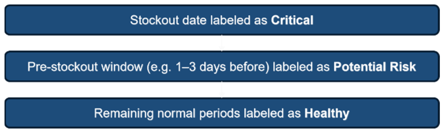
Critical	EIR > 0.18 or ITR > 2.0	High risk of stockout or overstock; corrective action required

thresholds were derived through multi-stage empirical calibration using historical stockout events from the training and calibration period as risk signals. Following the chronological partition in Section 3.1.6, the first 80% of observations was used for threshold calibration and the remaining 20% exclusively for independent diagnostic validation. As shown in Figure 6, calibration-period stockout dates were labeled “Critical,” the preceding three-day windows as “Potential Risk,” and other operational periods as “Healthy.”

The three-day pre-stockout window was selected as an interpretable short-term warning horizon to capture inventory deterioration immediately before stockout while excluding temporally distant observations, consistent with the one-day-ahead forecasting design. However, it is an empirically motivated rather than theoretically optimal choice, and alternative lead times should be evaluated through future ablation analysis.

A stockout event was defined as insufficient available inventory to satisfy observed demand. Isolated zero-demand observations were excluded due to intermittent retail demand. Only calibration-period observations meeting the stockout condition were used for threshold calibration, with no diagnostic validation data used for threshold estimation or calibration.

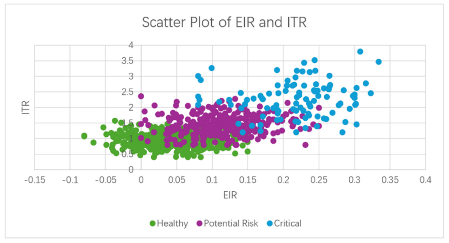
Event-labeled observations were mapped into the EIR–ITR space (Figure 7) to represent inventory risk around historical stockouts and their warning periods. Quantile analysis identified elevated imbalance in the upper-tail region, with the 80th–90th percentile range used as an empirical reference rather than a predetermined probability threshold. The resulting cutoffs were regularized into interpretable thresholds of EIR = 0.10 and 0.18 and ITR = 1.2 and 2.0. Positive EIR values indicate excess inventory relative to forecasted demand, whereas negative EIR values indicate potential understock conditions where expected demand exceeds available inventory. EIR is expressed as a proportion rather than a percentage; therefore, an EIR value of 0.10 corresponds to 10% and an EIR value of 0.18 corresponds to 18%.

The proposed diagnostic framework therefore distinguishes operational stockouts from naturally occurring zero-demand periods, ensuring that the thresholds reflect inventory risk rather than demand intermittency.

To ensure operational interpretability and account for the non-linear overlap between states, these specific quantile ranges from the calibration period were regularized into the finalized “clean” thresholds detailed in Table 11. These thresholds were fixed after calibration and subsequently applied unchanged to the independent diagnostic validation period. This empirical anchoring ensures that the diagnostic boundaries are not merely theoretical abstractions, but are directly informed by observed failure points and high-volatility periods in the calibration data.

The proposed thresholding framework is intended as a practical, data-driven diagnostic mechanism rather than a theoretically optimal classification model. By calibrating the thresholds using historical operational events from the calibration period and evaluating them on a subsequent independent validation period, the framework provides interpretable and operationally meaningful decision-support criteria for inventory health assessment. Although the thresholds were derived from a real-world industrial dataset, further validation using datasets from different retail environments will be an important direction for future research.

Although the thresholds were calibrated using a real-world industrial dataset, they should be regarded as empirically derived decision-support criteria rather than universally optimal values. To further evaluate the robustness of the calibrated thresholds, an additional sensitivity analysis was conducted exclusively on the independent diagnostic validation period by varying both the EIR and ITR thresholds by ±10%. Inventory health distributions remained largely consistent across tested settings, with over 60% of SKU–store combinations classified as Potential Risk or Critical in every scenario. This indicates robustness to moderate threshold variations, but does not directly validate diagnostic accuracy. Cross-domain validation using additional industrial datasets remains an important direction for future research.

Common thresholds were applied across all SKU–store combinations and categories to ensure consistent, comparable network-wide risk screening. Although subgroup-specific thresholds could better capture heterogeneity, they require sufficient event observations and substantially more calibration. Thus, the common thresholds provide a stable and interpretable baseline and should be viewed as empirical network-level decision-support criteria rather than universally optimal thresholds for individual products, stores, or categories.

3.4. Hyperparameter Optimization

To improve model robustness and avoid arbitrary parameter selection, a validation-based grid search procedure was conducted for RF, XGBoost, LSTM, and Transformer models. Candidate hyperparameter combinations were selected based on previous retail forecasting studies and preliminary experiments. The final parameter configuration for each model was determined according to the lowest validation RMSE.

For RF, the number of trees and maximum tree depth were optimized. For XGBoost, learning rate, tree depth, and the number of estimators were evaluated. For LSTM, the number of hidden units and dropout rate were optimized, while for Transformer, the number of attention heads and encoder layers were explored.

Table 12. Hyperparameter Search Space.

Model	Parameter	Search Space
RF	n_estimators	200, 400, 600
RF	max_depth	10, 20, 30
XGBoost	learning_rate	0.01, 0.05, 0.10
XGBoost	max_depth	4, 6, 8
XGBoost	n_estimators	500, 1000, 2000
LSTM	hidden units	32, 64, 128
LSTM	dropout	0.1, 0.2
Transformer	attention heads	2, 4, 8
Transformer	encoder layers	1, 2, 3

summarize the search spaces and the selected configurations.

3.5. Cross-Validation Strategy

To further assess forecasting robustness and model generalizability, a time-series-aware cross-validation procedure based on TimeSeriesSplit was employed. Unlike conventional random k-fold cross-validation, TimeSeriesSplit preserves temporal ordering and prevents information leakage from future observations into the training set.

Temporal cross-validation showed greater stability for LSTM (mean RMSE = 0.3655, SD = 0.0585) than Transformer (mean RMSE = 0.4487, SD = 0.3176), indicating higher Transformer sensitivity across folds. This instability may result from the short 14-day input window, heterogeneous SKU–store demand patterns, and greater Transformer complexity and data requirements. Thus, model complexity does not necessarily imply superior forecasting; LSTM provided a better balance of accuracy and stability for the present dataset.

Tree-based models (RF and XGBoost) were evaluated using 10-fold TimeSeriesSplit, while DL models (LSTM and Transformer) were evaluated using 5-fold TimeSeriesSplit due to their substantially higher computational cost. A series-level paired bootstrap analysis was conducted on the independent test period to assess statistical differences between models. SKU–store combinations were resampled with replacement, preserving within-series dependence, and paired performance differences were recalculated to construct 95% bootstrap intervals. These intervals distinguished descriptive performance differences from those supported by test-set sampling variability. Approximate 95% CIs for mean RMSE were calculated as mean RMSE ± 1.96 × (standard deviation/√k), where k is the number of validation folds. As the temporally ordered folds are not fully independent, these intervals represent approximate uncertainty rather than strict confidence intervals.

Table 13. Time-Series Cross-Validation Results.

Model	Validation Folds	Mean RMSE	Std RMSE	Approx. 95% Uncertainty Interval for Mean RMSE
RF	10	0.7985	0.0620	[0.7601, 0.8369]
XGBoost	10	0.7855	0.0880	[0.7309, 0.8401]
LSTM	5	0.3655	0.0585	[0.3142, 0.4168]
Transformer	5	0.4487	0.3176	[0.1703, 0.7271]

reports the mean RMSE, standard deviation, and corresponding intervals.

3.6. Evaluation Metrics

To rigorously evaluate the predictive performance of the candidate models and address RQ1, we employ a complementary set of evaluation metrics that captures absolute error, scale-normalized error, and relative percentage error. This multi-metric evaluation is particularly important for the high-volatility SKU–store dataset, which contains heterogeneous sales volumes and intermittent zero-demand observations. The following metrics are utilized to benchmark the six candidate models.

Root Mean Square Error (RMSE): Used to assess the magnitude of forecasting errors while assigning greater weight to large prediction deviations. As defined in (3), the squared error term makes RMSE particularly sensitive to large forecasting errors, including deviations occurring during high-demand periods. Therefore, RMSE is useful for evaluating whether a forecasting model can adequately accommodate demand peaks and other high-volatility periods:

$$\mathrm{R}\mathrm{S}\mathrm{M}\mathrm{E}=\sqrt{{\displaystyle \frac{1}{\mathrm{n}}}{\displaystyle \sum _{\mathrm{t}=1}^{\mathrm{n}}}({\mathrm{y}}_{\mathrm{t}}-{\widehat{\mathrm{y}}}_{\mathrm{t}}{)}^2}$$

(3)

Mean Absolute Percentage Error (MAPE): Measures the relative accuracy of the forecasts as a percentage of actual sales. By normalizing the error relative to the actual observed values, as expressed in (4), this metric allows for performance comparison across different product categories and store tiers regardless of their varying sales volumes:

$$\mathrm{M}\mathrm{A}\mathrm{P}\mathrm{E}={\displaystyle \frac{100\%}{\mathrm{n}}}{\displaystyle \sum _{\mathrm{t}=1}^{\mathrm{n}}}|{\displaystyle \frac{{\mathrm{y}}_{\mathrm{t}}-{\widehat{\mathrm{y}}}_{\mathrm{t}}}{{\mathrm{y}}_{\mathrm{t}}}}|$$

(4)

Because the dataset contains intermittent zero-demand observations, special treatment was applied during MAPE calculation. Observations with actual demand equal to zero were excluded from percentage-error computation because MAPE becomes mathematically undefined when the denominator equals zero. The proportion of excluded observations was relatively small (6.2% of the processed dataset), ensuring that the reported MAPE values remain representative of overall forecasting accuracy while avoiding numerical distortion caused by zero-demand periods.

MASE: Following the recommendations of [5], MASE serves as the primary metric for determining the “value-add” of advanced algorithmic models. By scaling the Mean Absolute Error (MAE) of a candidate model against the MAE of the SN baseline, as calculated in (5), a result of less than 1.00 confirms that the model provides superior predictive power over a simple seasonal heuristic:

$$\mathrm{M}\mathrm{A}\mathrm{S}\mathrm{E}={\displaystyle \frac{\frac{1}{\mathrm{n}}{\sum }_{\mathrm{i}=1}^{\mathrm{n}}|{\mathrm{y}}_{\mathrm{i}}-{\widehat{\mathrm{y}}}_{\mathrm{i}}|}{\frac{1}{\mathrm{n}-\mathrm{m}}{\sum }_{\mathrm{i}=\mathrm{m}+1}^{\mathrm{n}}|{\mathrm{y}}_{\mathrm{i}}-{\mathrm{y}}_{\mathrm{i}-\mathrm{m}}|}}$$

(5)

MAE: Measures the average absolute difference between the predicted and observed sales values. Unlike RMSE, MAE does not disproportionately penalize large errors and therefore provides an interpretable measure of the typical forecasting error in the original scale of the target variable.

$$\mathrm{M}\mathrm{A}\mathrm{E}={\displaystyle \frac{1}{\mathrm{n}}}{\displaystyle \sum _{\mathrm{i}=1}^{\mathrm{n}}}\left|{\mathrm{y}}_{\mathrm{i}}-{\widehat{\mathrm{y}}}_{\mathrm{i}}\right|$$

(6)

By integrating these complementary metrics, the study provides a multi-dimensional assessment of forecasting performance, allowing model strengths and weaknesses to be evaluated according to different error characteristics and operational objectives.

In this study, a seasonal period of seven days was adopted for MASE computation to reflect weekly demand seasonality. The same seasonal benchmark was consistently used for both the Seasonal Naïve forecasting model and the scaling series in the denominator, ensuring methodological consistency and interpretability of the reported MASE values.

4. Results and Discussion

The objective of this chapter is to evaluate the empirical performance of the proposed multi-layered forecasting and diagnostic framework. By analyzing approximately 500,000 product-store-day records from the dataset, this section provides a comparative assessment of the six candidate models defined in Section 3. The discussion transitions from the raw predictive accuracy of the models, measured through the standardized error metrics established in (3)–(5), to the operational utility of the Inventory Health Diagnostic Layer. This dual-focus approach ensures that the value-add of advanced architectures, such as the Transformer and LSTM, is quantified not only in terms of statistical precision but also in their ability to mitigate systemic supply chain risks during high-volatility promotional periods.

4.1. Predictive Performance Benchmarking

The predictive performance of the six candidate models was evaluated to address RQ1, focusing on their ability to navigate the non-linear demand spikes inherent in multi-category retail. By benchmarking the statistical baselines against the ensemble and DL models, we can identify the specific algorithmic strengths required for modern SKU-level management. The consolidated results for the testing period are presented in

Table 14. Comparative Performance Metrics for Demand Forecasting Models.

Model	RMSE	MAPE (%)	MASE	MAE
SN	2.2353	156.24%	1.0000	1.3526
Prophet	0.5504	34.66	1.3405	0.4413
RF	0.7586	63.69	0.5368	0.6077
XGBoost	0.7683	62.52	0.5309	0.6138
LSTM	0.3996	21.63	0.8595	0.3189
Transformer	0.4698	27.32	1.1030	0.3752

.

4.1.1. Comparative Evaluation of Forecasting Accuracy

The experimental results indicate that the LSTM model achieved the strongest point-estimate performance in terms of RMSE and MAPE, while XGBoost achieved the lowest MASE. Specifically, LSTM obtained the lowest testing RMSE (0.3996) and MAPE (21.63%), whereas RF and XGBoost produced lower MASE values than the other advanced models. Overall, model performance depended on the evaluation criterion. Cross-validation showed that LSTM achieved the lowest mean RMSE (0.3655; approximate 95% CI: [0.3142, 0.4168]), while Transformer had a higher mean RMSE (0.4487) and wider interval ([0.1703, 0.7271]), indicating greater variability across temporal folds. RF and XGBoost showed similar performance, with overlapping intervals ([0.7601, 0.8369] and [0.7309, 0.8401], respectively), so their RMSE difference should not be interpreted as statistically significant. Overall, considering both performance and variability, LSTM showed the most favorable results under RMSE and MAPE, while differences among competing models should be interpreted cautiously.

4.1.2. Technical Interpretation of Model Performance Differences

Table 13 and Table 14 show that model performance varied across error metrics and temporal folds. LSTM achieved the lowest testing RMSE and MAPE and the lowest cross-validation mean RMSE, while RF and XGBoost achieved substantially lower MASE values. Thus, no model was uniformly superior across all evaluation criteria. This interpretation reflects the observed estimates and cross-validation variability without assuming that all model differences are statistically significant.

Capture of Long-Range Temporal Dependencies: Unlike the SN baseline, which relies on a fixed weekly seasonal pattern, LSTM uses its gated recurrent architecture and 14-day input window to capture short-term demand persistence, weekly fluctuations, and recent promotional changes, achieving the lowest testing RMSE (0.3996). However, the 14-day window limits its ability to explicitly capture long-term annual or multi-month dependencies.

Robustness to High-Volatility Shocks: While XGBoost and RF are effective at partitioning heterogeneous tabular features, their higher MAPE values indicate greater relative errors for low-volume observations. In contrast, the Transformer architecture uses multi-head self-attention to model relationships among historical observations. However, its wider cross-validation confidence interval indicates greater variability across temporal folds, suggesting that higher architectural complexity does not necessarily improve performance stability.

Mitigation of Zero-Inflation and Noise: The SKU-store dataset is characterized by sparse intervals and high-frequency noise. The results indicate that LSTM provides a favorable combination of RMSE and MAPE performance in this setting, while RF and XGBoost provide stronger scaled-error performance according to MASE. Therefore, the observed results reflect different performance profiles rather than a uniformly dominant architecture. Nevertheless, model differences should be interpreted alongside their confidence intervals and not considered statistically significant without a formal paired test.

4.2. Operational Validation of the Inventory Health Diagnostic Layer

While the previous section established the statistical performance of the forecasting models, the practical utility of the framework depends on its ability to translate these forecasts into actionable inventory management signals. This section evaluates the Inventory Health Diagnostic Layer using the independent diagnostic validation period. The thresholds derived exclusively from the preceding calibration period were applied to the forecasted demand and inventory observations in the validation period without further adjustment. By shifting the focus from error percentages to the actual distribution of stock health, we can evaluate the system’s ability to identify systemic risks, such as capital stagnation and stockout potential, on previously unseen observations.

4.2.1. System-Wide Distribution of SKU-Store Health States

The second phase of the experimental evaluation translates the forecasting outputs into actionable operational insights through the diagnostic layer. By applying the event-calibrated thresholds established in Table 11, each SKU–store combination was categorized into one of three health states. The results, summarized in

Table 15. Distribution of Inventory Health States across SKU–Store Combinations.

Health Level	Diagnostic Condition	Interpretation
Healthy	38.9	Balanced supply and demand
Potential Risk	44.8	Early warning of misalignment
Critical	16.3	Immediate intervention required

, reveal a significant structural imbalance within the supply chain. The analysis indicates that only 38.9% of inventory positions are classified as Healthy, suggesting that current replenishment strategies are not fully synchronized with localized demand patterns. More critically, over 60% of the dataset exhibits some form of inventory risk, with 16.3% categorized as Critical. The robustness of the calibrated threshold selection was further examined through a sensitivity analysis conducted exclusively on the independent validation period. The overall distribution of inventory health states changed only marginally under moderate threshold perturbations, and the proportion of inventory classified as Potential Risk or Critical consistently remained above 60%. These findings indicate that the proposed diagnostic conclusions are stable and are not driven solely by the observations used during threshold calibration or by a particular threshold configuration. These “Critical” cases represent high-risk stockout or overstocking scenarios that warrant managerial attention, with possible interventions including emergency replenishment or markdown consideration to prevent lost sales and capital stagnation. The diagnostic framework provides early warnings, enabling managers to prioritize high-risk SKU–store combinations before inventory risks escalate into serious operational problems.

Threshold calibration used a three-day pre-stockout window, the 80th–90th percentile EIR–ITR region, and rectangular boundaries for interpretable network-wide screening. Although not globally optimal, ±10% sensitivity analysis showed stable diagnostic-state distributions, supporting robustness. Further ablation of warning windows, quantile ranges, and category-specific or nonlinear boundaries is needed for optimization.

4.2.2. ITR and EIR Indicators

To understand the drivers behind the “Critical” and “Potential Risk” states, it is necessary to examine the interaction between capital velocity (ITR) and stock surplus (EIR). The diagnostic layer utilizes these two metrics as a coordinate system to delineate the boundaries of operational health. As shown in the coordinate mapping in Figure 7, the dataset exhibits a high degree of variance in turnover efficiency. The average ITR of 2.22 indicates a relatively high inventory position compared with realized sales, suggesting slow circulation and potential inventory accumulation. The mean EIR of −0.40 indicates that forecasted demand generally exceeded available inventory, suggesting under-provisioning across much of the network, although some SKU–store combinations show positive EIR values indicating excess inventory. The clustering of data points in the Critical region (ITR > 2.0 or EIR > 0.18) highlights specific store-category combinations where high demand volatility has outpaced traditional replenishment logic. By identifying these clusters, the framework provides managers with a targeted intervention list, prioritizing SKUs that contribute most to capital stagnation. This diagnostic granularity ensures that corrective actions, such as inter-store stock transfers or localized markdowns, are data-driven rather than reactive.

4.2.3. Synthesis of Stockout and Obsolescence Risks

The final validation of the diagnostic layer involves assessing its ability to distinguish between different modes of supply chain failure. By cross-referencing the state distribution from Table 15 with temporal sales patterns, the framework identifies two primary risks: stockout probability and inventory obsolescence. As summarized in the diagnostic findings, 16.3% of SKU–store observations in the independent diagnostic validation period were classified as Critical. Analysis through the lens of the EIR and ITR provides further insight into the potential understock and overstock conditions represented by these high-risk observations. Conversely, SKU–store combinations with ITR values substantially above the 2.0 threshold indicate a higher risk of inventory accumulation and aging due to relatively high inventory levels compared with realized sales. This is particularly prevalent in non-seasonal categories where the lack of demand-responsive replenishment has led to capital being “trapped” in low-velocity stock. The integration of the LSTM’s predictive signals with these diagnostic triggers allows the system to generate a prioritized risk matrix. Rather than prescribing an optimized replenishment policy, the framework associates different inventory-risk states with rule-based managerial recommendations based on the severity and direction of the EIR/ITR signals. For instance, SKUs identified as “Critical-Understock” can be flagged for managerial consideration of expedited replenishment, while those identified as “Potential-Overstock” can be prioritized for managerial consideration of promotional interventions to reduce the risk of aging stock. These recommendations are intended to support managerial prioritization rather than automatically determine an optimal course of action. Therefore, the framework should be understood as a predictive-to-diagnostic decision-support system rather than a fully prescriptive inventory optimization tool.

4.2.4. Overall Discussion

The forecasting results reveal clear performance differences among the evaluated model families. LSTM achieved the lowest RMSE and MAPE values, indicating its strong ability to capture temporal dependencies and nonlinear demand fluctuations within SKU–store sales sequences. This advantage is particularly beneficial in retail environments characterized by seasonality, promotional activities, and irregular demand patterns. The Transformer showed weaker performance, possibly due to the short 14-day input window and one-day forecasting horizon, which may limit the benefits of self-attention. Thus, these results reflect its performance under this short-term configuration rather than its general forecasting capability.

Overall, the results indicate that forecasting performance depends on the evaluation metric adopted. LSTM has lowest RMSE and MAPE, while RF and XGBoost achieved more favorable MASE values. Therefore, no single model consistently outperformed all competing approaches across every evaluation metric, highlighting the importance of selecting models according to specific operational objectives.

4.3. Discussion and Literature Comparison

The experimental findings of this study offer a dual contribution to the retail analytics literature by examining the comparative performance of statistical, ML, and DL forecasting models for high-frequency demand forecasting and demonstrating the operational value of an integrated, event-calibrated diagnostic system. This section benchmarks these results against existing research and discusses the broader implications for modern retail management. To clearly delineate the contributions of this research relative to established benchmarks,

Table 16. Comparison of the Proposed Work with State-of-the-Art Approaches.

Ref.	Methodology	Key Focus	Forecasting Performance	Operational Diagnostic Link
[20]	LSTM	M5 Walmart Benchmark	High (RMSE: 0.289)	No (Purely Predictive)
[1]	Transformer	UK Retail Benchmarking	High (MAPE: 6.1%)	Limited (Theoretical)
[21]	LSTM/RNN	Supermarket Daily Sales	High (RMSE: 1.55)	No (Forecasting Only)
This Work	LSTM & Integrated Framework	E-commerce Risk Assessment	High (RMSE: 0.3996)	Yes (Event-Calibrated)

provides a summary of representative studies from literature. While these works demonstrate state-of-the-art predictive performance, this study is unique in its integration of those predictive signals into a localized diagnostic framework for inventory health.

4.3.1. Alignment with Modern Forecasting Literature

The strong RMSE and MAPE performance of the LSTM model in this study, with the lowest testing RMSE (0.3996) and MAPE (21.63%), is consistent with previous evidence that recurrent architectures can perform well in retail demand forecasting. Our results corroborate the findings of [6,7], who noted that gated recurrent units and self-attention mechanisms are uniquely suited for capturing the non-linear “shocks” caused by retail promotions. Furthermore, our observation that the Transformer’s performance was slightly more sensitive to data noise (MASE: 1.1030) compared to the LSTM supports the assertion by [30] that recurrent architectures often maintain better stability in the presence of the “zero-inflation” common in SKU-level datasets.

4.3.2. Bridging the Predictive-Prescriptive Gap

A significant finding of this research is the successful integration of point forecasts into an actionable diagnostic framework, addressing the “operational silo” identified by [1,2]. As illustrated in Table 16, most existing research focuses exclusively on improving error metrics like RMSE and MAPE. By contrast, our framework uses the forecasting outputs, including those generated by the LSTM model, not as an end in themselves, but as inputs to the event-calibrated diagnostic process described in Section 3.3. This approach demonstrates how forecasting outputs can be systematically transformed into interpretable inventory-risk and decision-support signals through rule-based diagnostic logic. The identification of over 60% of inventory records as having “Potential” or “Critical” risk underscores the limitations of the “memoryless” replenishment systems currently used in the industry, which lack the forward-looking capacity of our integrated system.

4.3.3. Contextual Robustness and Scalability

Unlike previous studies that focus on single-category or small-scale datasets, our framework’s performance across 500,000 multi-city records demonstrates its scalability. By incorporating contextual features such as city tier and promotion flags (as detailed in Section 3.1), the framework accounts for the geographical and category-specific heterogeneity often ignored in more aggregate-level research. These results provide empirical evidence that the proposed framework can be applied to large-scale, multi-branch e-commerce data and can serve as a basis for an operational diagnostic dashboard. However, practical deployment and external validation would be required before generalizing this conclusion to other retail environments.

5. Conclusions and Future Work

This study has presented an integrated framework for retail demand forecasting and inventory health diagnosis, validated through a comprehensive empirical analysis of 500,000 product-store-day records from the Hengyuansheng (Quanzhou) Digital Technology Co., Ltd. Addressing the core RQs, the results show that model performance varied across evaluation criteria. LSTM achieved the lowest testing RMSE (0.3996) and MAPE (21.63%), while XGBoost and RF achieved lower MASE values, indicating no single model dominated across all metrics. The forecasting results provide predictive input to the integrated diagnostic layer, bridging statistical prediction and interpretable inventory decision support. By utilizing event-calibrated thresholds derived exclusively from historical stockout signals in the calibration period, the framework was independently evaluated on the subsequent validation period. The results show that 61.1% of SKU–store observations in the independent validation period were classified as Potential Risk or Critical, with 16.3% categorized as Critical. These findings demonstrate the ability of the framework to transform forecasting outputs into transparent and interpretable inventory health signals on previously unseen observations.

From a managerial perspective, the implications of this research are significant for the transition toward data-driven, proactive supply chain oversight. The proposed diagnostic dashboard allows retail practitioners to move beyond reactive troubleshooting by prioritizing high-risk SKUs and implementing targeted interventions, such as expedited replenishment or strategic markdowns, before capital stagnation or stockouts occur. The proposed inventory health diagnostic framework can assist managers in prioritizing high-risk SKUs, monitoring inventory status, and allocating resources more effectively, thereby supporting operational decision-making. However, the framework does not perform formal replenishment optimization, which would require an explicit decision model incorporating costs, lead times, service levels, replenishment quantities, capacity constraints, and demand uncertainty. The robustness of the system is particularly evident during high-volatility promotional windows, where the event-calibrated logic prevents the “false alarms” often triggered by traditional, static replenishment systems. Ultimately, this framework provides a scalable and interpretable solution for large-scale e-commerce enterprises seeking to synchronize their inventory levels with localized, time-sensitive demand patterns.

Despite these contributions, certain limitations suggest productive avenues for future research. While the current system utilizes a fixed historical sequence window, future iterations could incorporate dynamic window sizes to better accommodate varying product lifecycles across different retail categories. Furthermore, the integration of unsupervised anomaly detection techniques, such as Isolation Forest or One-Class SVM, could refine the system’s ability to detect irregular stock movements like “phantom inventory” or sudden data drift. Finally, expanding the framework to encompass multi-echelon optimization would enable automated stock rebalancing between city branches, further enhancing the resilience and efficiency of the broader supply chain network. Although the proposed thresholds were calibrated using historical inventory events from the study dataset and evaluated on a temporally independent validation period, external validation using independent retail datasets was not conducted in this study. Therefore, the generalizability of the threshold values beyond the studied retail environment remains to be established. While the sensitivity analysis provides evidence of within-dataset robustness, it cannot replace cross-domain or cross-company validation. Future research will therefore focus on validating the proposed threshold calibration strategy using independent datasets from diverse retail environments, product categories, and operational settings. Such external validation will help determine whether the identified threshold ranges remain stable across different inventory structures and demand characteristics or require context-specific recalibration. In addition, future work will investigate more advanced inventory risk modeling techniques and evaluate the operational impact of the diagnostic signals through real-world or controlled decision-support experiments.

Future research will extend the forecasting benchmark to specialized contemporary and advanced time-series models to assess whether more complex architectures improve predictive performance and downstream inventory diagnostics across different forecasting horizons and retail environments.

References

1. Fildes, R.; Ma, S.; Kolassa, S. Retail Forecasting: Research and Practice. Int. J. Forecast. 2022, 38, 1283–1318. [Google Scholar] [CrossRef] [Scilit]
2. Aro, O.E.; Louis, S. Framework for Evaluating Inventory Health. Int. J. Humanit. Soc. Sci. Manag. 2024, 4, 82–86. [Google Scholar]
3. Ren, S.; Chan, H.L.; Siqin, T. Demand Forecasting in Retail Operations for Fashionable Products: Methods, Practices, and Real Case Study. Ann. Oper. Res. 2020, 291, 761–777. [Google Scholar] [CrossRef] [Scilit]
4. Ma, S.; Fildes, R.; Huang, T. Demand Forecasting with High Dimensional Data: The Case of SKU Retail Sales Forecasting with Intra- and Inter-Category Promotional Information. Eur. J. Oper. Res. 2016, 249, 245–257. [Google Scholar] [CrossRef] [Scilit]
5. Hyndman, R.J.; Athanasopoulos, G. Forecasting, 3rd ed.; OTexts: Melbourne, Australia, 2021. [Google Scholar]
6. Punia, S.; Nikolopoulos, K.; Singh, S.P.; Madaan, J.K.; Litsiou, K. Deep Learning with Long Short-Term Memory Networks and Random Forests for Demand Forecasting in Multi-Channel Retail. Int. J. Prod. Res. 2020, 58, 4964–4979. [Google Scholar] [CrossRef] [Scilit]
7. Oliveira, J.M.; Ramos, P. Evaluating the Effectiveness of Time Series Transformers for Demand Forecasting in Retail. Mathematics 2024, 12, 2728. [Google Scholar] [CrossRef] [Scilit]
8. Bhatt, A.P.; Nahar, P. Smart Retail Inventory Management Using AI-Driven IoT. J. Supply Chain Manag. Syst. 2025, 14, 30–36. [Google Scholar] [CrossRef] [Scilit]
9. Falatouri, T.; Darbanian, F.; Brandtner, P.; Udokwu, C. Predictive Analytics for Demand Forecasting—A Comparison of SARIMA and LSTM in Retail SCM. Procedia Comput. Sci. 2022, 200, 993–1003. [Google Scholar] [CrossRef] [Scilit]
10. Auppakorn, C.; Phumchusri, N. Daily Sales Forecasting for Variable-Priced Items in Retail Business. In Proceedings of the ACM International Conference Proceeding Series, Chiang Mai, Thailand, 28 April 2022; Association for Computing Machinery: New York, NY, USA, 2022; pp. 80–86. [Google Scholar]
11. Makridakis, S.; Spiliotis, E.; Assimakopoulos, V. M5 Accuracy Competition: Results, Findings, and Conclusions. Int. J. Forecast. 2022, 38, 1346–1364. [Google Scholar] [CrossRef] [Scilit]
12. Kao, C.Y.; Chueh, H.E. Deep Learning Based Purchase Forecasting for Food Producer-Retailer Team Merchandising. Sci. Program. 2022, 2022, 2857850. [Google Scholar] [CrossRef] [Scilit]
13. Mitra, A.; Jain, A.; Kishore, A.; Kumar, P. A Comparative Study of Demand Forecasting Models for a Multi-Channel Retail Company: A Novel Hybrid Machine Learning Approach. Oper. Res. Forum 2022, 3, 58. [Google Scholar] [CrossRef] [Scilit]
14. Chen, I.F.; Lu, C.J. Sales Forecasting by Combining Clustering and Machine-Learning Techniques for Computer Retailing. Neural Comput. Appl. 2017, 28, 2633–2647. [Google Scholar] [CrossRef] [Scilit]
15. Krishna, A.; Akhilesh, V.; Aich, A.; Hegde, C. Sales-Forecasting of Retail Stores Using Machine Techniques; IEEE: Bengaluru, India, 2018. [Google Scholar]
16. Kohli, S.; Godwin, G.T.; Urolagin, S. Sales Prediction Using Linear and KNN Regression; Springer: Berlin/Heidelberg, Germany, 2021; pp. 321–329. [Google Scholar]
17. Ganguly, P.; Mukherjee, I. Enhancing Retail Sales Forecasting with Optimized Machine Learning Models. In Proceedings of the 4th International Conference on Sustainable Expert Systems, ICSES 2024, Kaski, Nepal, 15–17 October 2024; Institute of Electrical and Electronics Engineers: Piscataway, NJ, USA, 2024; pp. 884–889. [Google Scholar] [CrossRef] [Scilit]
18. Ahmed, R.S.; Hasnain, M.; Mahmood, M.H.; Mehmood, M.A. Comparison of Deep Learning Algorithms for Retail Sales Forecasting. ICCK Trans. Intell. Syst. 2024, 1, 112–126. [Google Scholar] [CrossRef] [Scilit]
19. Mao, H.; Gao, Z.; Hou, J. Research on E-Commerce Retail Demand Forecasting Based on Multi-Model Fusion. Highlights Bus. Econ. Manag. 2025, 55, 113–121. [Google Scholar] [CrossRef] [Scilit]
20. Hewamalage, H.; Montero-Manso, P.; Bergmeir, C.; Hyndman, R.J. A Look at the Evaluation Setup of the M5 Forecasting Competition. arXiv 2021, arXiv:2108.03588. [Google Scholar] [CrossRef] [Scilit]
21. Pinochet, L.H.C.; de Souza, C.A.; Viana, A.B.N.; Rodríguez-Abitia, G.; Pardim, V.I. Predicting the Antecedents of Quality of Life from the Use of Smart Technologies in Supermarket Retail: An in-Depth Investigation Using Artificial Neural Networks. In Proceedings of the Procedia Computer Science; Elsevier B.V.: Amsterdam, The Netherlands, 2023; Volume 221, pp. 450–457. [Google Scholar]
22. Lim, B.; Zohren, S. Time-Series Forecasting with Deep Learning: A Survey. Philos. Trans. R. Soc. A 2021, 379, 20200209. [Google Scholar] [CrossRef] [Scilit] [PubMed]
23. Punia, S.; Shankar, S. Predictive Analytics for Demand Forecasting: A Deep Learning-Based Decision Support System. Knowl. Based. Syst. 2022, 258, 109956. [Google Scholar] [CrossRef] [Scilit]
24. Giri, C.; Chen, Y. Deep Learning for Demand Forecasting in the Fashion and Apparel Retail Industry. Forecasting 2022, 4, 565–581. [Google Scholar] [CrossRef] [Scilit]
25. Perin, J.; Sampaio, L.; Marcon, M.; Ortoncelli, A. Prediction of Daily Sales of Individual Products in a Medium-Sized Brazilian Supermarket Using Recurrent Neural Networks Models. In Proceedings of the 14th International Conference on Data Science, Technology and Applications, Bilbao, Spain, 10–12 June 2025; SCITEPRESS: Setúbal, Portugal, 2025; pp. 739–747. [Google Scholar] [CrossRef] [Scilit]
26. Li, C.; Cheang, B.; Luo, Z.; Lim, A. An Exponential Factorization Machine with Percentage Error Minimization to Retail Sales Forecasting. ACM Trans. Knowl. Discov. Data 2021, 15, 22. [Google Scholar] [CrossRef] [Scilit]
27. Guha, A.; Grewal, D.; Kopalle, P.K.; Haenlein, M.; Schneider, M.J.; Jung, H.; Moustafa, R.; Hegde, D.R.; Hawkins, G. How Artificial Intelligence Will Affect the Future of Retailing. J. Retail. 2021, 97, 28–41. [Google Scholar] [CrossRef] [Scilit]
28. Yousaf, M.; Dehning, B. The Effects of Sales Surprise on Inventory Turnover: An Empirical Study. Cogent Econ. Financ. 2023, 11, 2258696. [Google Scholar] [CrossRef] [Scilit]
29. Kourentzes, N.; Trapero, J.R.; Barrow, D.K. Optimising Forecasting Models for Inventory Planning. Int. J. Prod. Econ. 2020, 225, 107597. [Google Scholar] [CrossRef] [Scilit]
30. Nasseri, M.; Falatouri, T.; Brandtner, P.; Darbanian, F. Applying Machine Learning in Retail Demand Prediction—A Comparison of Tree-Based Ensembles and Long Short-Term Memory-Based Deep Learning. Appl. Sci. 2023, 13, 11112. [Google Scholar] [CrossRef] [Scilit]
Figure 1. Proposed Research Framework.
Information 17 00909 g001
Figure 2. Price Distribution (Unit: RMB).
Information 17 00909 g002
Figure 3. Median Sale Amount of Cities.
Information 17 00909 g003
Figure 4. Total Sale Amount of First Categories.
Information 17 00909 g004
Figure 5. Sales Volume Representation by City.
Information 17 00909 g005
Figure 6. Event-Driven Inventory State Labeling Process.
Information 17 00909 g006
Figure 7. Inventory Health Diagnostic Logic and State Distribution.
Information 17 00909 g007