Knowledge-Guided Multimodal Resource Identification in Low-Voltage Transformer Areas with Sparse Measurements

Abstract

Identifying distributed photovoltaic generation, battery energy storage, and load-dominant behaviour remains challenging when transformer-area measurements are sparse, operating patterns overlap, and reference labels are incomplete. We develop a knowledge-guided multimodal learning framework that combines raw electrical sequences with temporal, statistical, frequency-domain, and contextual descriptors. A knowledge-guided label library reconciles archived operating records, expert rules, and clustering-based screening, while transfer learning and WGAN-based augmentation are used to improve learning under limited and imbalanced data. The proposed framework jointly encodes raw electrical sequences, engineered descriptors, and contextual information and integrates their complementary representations through attention-based multimodal fusion. On a held-out real-only test set with independently verified labels, the proposed framework achieved 93.8% accuracy and a macro-F1 of 93.8%, while retaining 90.4% accuracy when 30% of the inputs were randomly masked. These results support further evaluation of knowledge-guided multimodal learning for transformer-area resource identification, although broader cross-region and cross-utility validation is required before operational deployment.

1. Introduction

Distributed energy resources (DERs), particularly rooftop photovoltaic (PV) systems and small-scale battery energy storage systems (BESSs), are altering power flows in low-voltage distribution networks. Within a transformer area, residential and commercial demand may coincide with PV generation, storage operation, and variable user responses. Their overlapping signatures complicate line-loss analysis, resource monitoring, anomaly localisation, and hosting-capacity assessment [1,2]. Reliable identification of the dominant resource pattern is therefore becoming an important component of transformer-area observability [3,4].

Previous work has examined supply–demand balance identification in PV-rich transformer areas and storage control for renewable-energy accommodation [5,6]. Coordinated control of charging stations and DERs provides a complementary route to local flexibility [7]. Other studies have used multidimensional features for anomaly detection and line-loss estimation in noisy transformer-area data [8,9,10]. Related research on power quality and PV optimisation further illustrates the value of distinguishing generation- and load-side behaviour [11,12]. In practice, however, communication constraints and asynchronous data streams continue to limit measurement quality and temporal alignment [13,14].

Three limitations remain. First, many methods rely on a single electrical quantity and therefore capture only part of the relationship among resource composition, temporal dynamics, and power-quality signatures. Second, sparse or asynchronous acquisition introduces missing values and temporal misalignment that can destabilise feature extraction [8,15]. Third, transformer-area datasets are often small, imbalanced, and weakly labelled, which limits model transfer to new regions and uncommon operating states [16,17,18].

Here, we investigate whether operational knowledge and multimodal learning can be combined to identify transformer-area resource patterns from sparse measurements. The framework uses a knowledge-guided label library to screen weak labels and then combines raw sequences, engineered electrical features, and contextual descriptors. This design separates label curation from representation learning and provides an explicit operational basis for interpreting the model inputs and decisions.

Related Work and Remaining Gap

Transformer-area analytics has developed along three related lines. The first addresses individual operational tasks, including supply–demand balance identification, line-loss analysis, and hosting-capacity evaluation [3,5,8,9]. The second supports specific resources through PV optimisation, storage control, and power-quality assessment [4,6,11,12]. The third considers imperfect data through transfer learning, data repair, and streaming-data processing [14,16,17,18]. Recent studies have also examined weakly supervised transformer-area identification, multi-feature topology decisions, and GAN-based robustness under missing or imbalanced data [19,20,21]. These studies establish the relevant components, but their joint use for transformer-area resource classification remains insufficiently evaluated. In particular, the interaction between weak-label screening, multimodal fusion, and robustness to sparse measurements has received limited attention.

The study makes the following contributions:

• A multidimensional representation combines temporal, statistical, and spectral information from transformer-area electrical measurements.
• A knowledge-guided label library screens uncertain labels using historical records, operational rules, and clustering evidence.
• Transfer learning and WGAN-based augmentation are incorporated to address limited and imbalanced training data.
• A CNN–LSTM–Attention architecture fuses electrical sequences, engineered features, and contextual descriptors.
• A pilot case study evaluates the framework against conventional machine-learning, recurrent, convolutional, and recent Transformer-based time-series baselines on a held-out real-only test set.

Section 2 describes the problem formulation, feature construction, label library, and model architecture. Section 3 presents the case study and evaluation protocol. Section 4 reports and interprets the results, and Section 5 concludes the paper.

2. Materials and Methods

2.1. Problem Formulation

Transformer-area resource identification was formulated as a four-class classification problem at the observation-window level. Each window contained $T=96$ time steps, corresponding to one day of measurements sampled at 15 min intervals. The input comprised aggregated electrical measurements and auxiliary descriptors, and the output represented the dominant resource composition or operating pattern.

Four representative classes were considered. Load-dominant windows lacked pronounced DER signatures, whereas PV-associated windows showed reverse-flow or midday generation patterns. Storage-associated windows exhibited charging or discharging signatures, and mixed-resource windows combined PV, storage, and load behaviour. The class definitions were chosen for transformer-area screening and resource monitoring [22].

2.2. Multidimensional Feature Construction

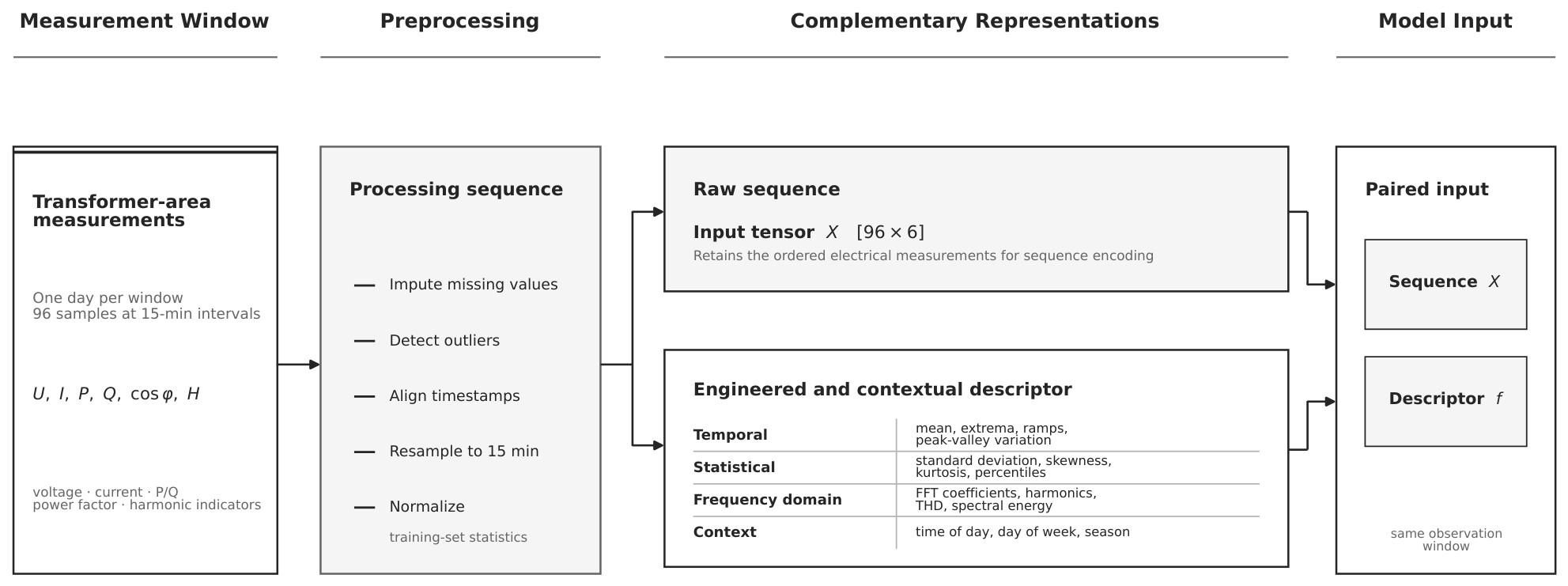
The model combined raw sequences with engineered descriptors to distinguish overlapping resource patterns. At time step t, the raw measurement vector was defined as

$${\mathbf{x}}_t={[U_t,I_t,P_t,Q_t,\cos {\phi }_t,H_t]}^{\top },$$

(1)

where $U_t$ is voltage, $I_t$ is current, $P_t$ is active power, $Q_t$ is reactive power, $\cos {\phi }_t$ is power factor, and $H_t$ denotes harmonic-related variables.

Engineered features were extracted in three groups:

• Temporal features. Means, extrema, ramp rates, peak–valley differences, and sliding-window variation coefficients described trend, variability, and periodicity.
• Statistical distribution features. Standard deviation, skewness, kurtosis, percentile spread, and outlier ratio characterised the shape and dispersion of each window.
• Frequency-domain and power-quality features. Fast Fourier transform (FFT) coefficients, harmonic content, total harmonic distortion (THD), and spectral energy described inverter-related and conventional load signatures.

The resulting descriptor vector is written as

$$\mathbf{f}=[{\mathbf{f}}_{\mathrm{time}},{\mathbf{f}}_{\mathrm{stat}},{\mathbf{f}}_{\mathrm{freq}},{\mathbf{f}}_{\mathrm{ctx}}],$$

(2)

where ${\mathbf{f}}_{\mathrm{ctx}}$ contains time-of-day, day-of-week, and seasonal descriptors.

Figure 1 illustrates the multidimensional feature-construction workflow.

2.3. Knowledge-Guided Label Library Construction

Reference labels were assembled from three sources: archived operating records, expert-defined electrical rules, and clustering of weakly labelled or unlabelled samples [22,23]. Archived records served as anchors when their timestamps and operating context were considered reliable. Expert rules then assigned candidate labels and confidence scores using directional power flow, ramp rates, power factor, and harmonic cues. Clustering of feature embeddings identified compact pattern groups and samples whose neighbourhood disagreed with the candidate label.

Samples were accepted when archived records and rule-based labels agreed. For samples without reliable archived records, each applicable electrical cue contributed one binary support vote to the candidate class. The rule-based confidence score for sample i was therefore

$$C_i={\displaystyle \frac{n_i^{\mathrm{support}}}{n_i^{\mathrm{applicable}}}},$$

(3)

where $n_i^{\mathrm{support}}$ is the number of applicable cues supporting the candidate class, and $n_i^{\mathrm{applicable}}$ is the total number of applicable cues. Candidate labels with $C_i\ge 0.75$ were retained. K-means clustering with $K=4$ was applied to the feature embeddings. For cluster k, purity was defined as

$${\mathrm{Purity}}_k=\underset{c}{\max }{\displaystyle \frac{n_{k,c}}{N_k}},$$

(4)

where $n_{k,c}$ is the number of samples assigned to class c in cluster k, and $N_k$ is the cluster size. Clusters with purity $\ge 0.80$ were regarded as reliable. Samples failing these criteria or showing disagreement between the rule-based and clustering results were marked as ambiguous and excluded from supervised optimisation. Among the 6720 real candidate windows in the training and validation subsets, 480 were identified as ambiguous, while 6240 passed the screening procedure: 1820 load-dominant, 1517 PV-associated, 910 storage-associated, and 1993 mixed-resource windows. The ambiguous samples were retained only for manual review and error analysis. Thus, the knowledge-guided label library supported label assignment, conflict screening, training-sample selection, and post-hoc interpretation rather than acting as a fixed classifier.

The knowledge-guided labelling procedure was applied to the construction and screening of the training and validation samples. For model evaluation, the labels of the held-out real test samples were independently verified using transformer-area equipment installation information, utility asset records, and corresponding operating records.

Table 1. Operational cues used by the knowledge-guided pilot label library.

Class	Indicative Operational Cues
Load-dominant	No persistent reverse power flow; daily pattern mainly follows demand-side peak and valley behaviour; harmonic and reactive features remain consistent with conventional aggregated load operation.
PV-associated	Midday active-power depression or reverse-flow tendency; daytime voltage rise and harmonic signatures consistent with inverter-connected generation; solar-period correlation.
Storage-associated	Repeated bidirectional ramping and state-transition behaviour; charging/discharging signatures appear at valley-filling or peak-shaving periods; local power-factor and harmonic variation differ from purely passive load.
Mixed-resource	Simultaneous presence of PV-like daytime behaviour and storage-like bidirectional adjustment; partial overlap between generation and flexible load or storage response.

summarises the operational cues used in the pilot study. Because these cues depend on metering resolution, transformer-area scale, and local equipment characteristics, their operating thresholds require recalibration before transfer to a different deployment setting.

Preprocessing comprised missing-value treatment, robust outlier screening, timestamp alignment, resampling, and normalisation. Short consecutive gaps were repaired by linear interpolation, whereas longer recoverable gaps were estimated from measurements at the corresponding time of day on recent valid days from the same transformer area. Observation windows with excessive missingness were excluded from subsequent analysis. Outliers were jointly identified using an interquartile-range-based distributional criterion and a Hampel local-consistency filter. Values identified as abnormal by both criteria were treated as missing observations and repaired using the same imputation procedure. Finally, all measurement channels were aligned to 15 min timestamps, and continuous variables were standardised using statistics calculated exclusively from the training subset.

2.4. Simulation- and WGAN-Based Data Augmentation and Transfer Learning

Simulation-assisted samples were generated from representative daily profiles derived exclusively from the real training data to supplement rare or underrepresented operating states. Load profiles were produced by amplitude scaling, temporal shifting, and stochastic perturbation according to

$$P_L^{\mathrm{sim}}\left(t\right)=a_L{P}_L^{\mathrm{ref}}(t+\Delta t)+{ϵ}_t,$$

(5)

where $P_L^{\mathrm{ref}}\left(t\right)$ denotes a representative daily load profile, $a_L$ is the amplitude-scaling factor, $\Delta t$ denotes the temporal shift of the daily pattern, and ${ϵ}_t$ represents a small stochastic perturbation. PV profiles were generated by scaling representative PV profiles,

$$P_{\mathrm{PV}}^{\mathrm{sim}}\left(t\right)=a_{\mathrm{PV}}{P}_{\mathrm{PV}}^{\mathrm{ref}}\left(t\right),\hspace{1em}{P}_{\mathrm{PV}}^{\mathrm{sim}}\left(t\right)\ge 0,$$

(6)

where $a_{\mathrm{PV}}$ controls the PV output scale. BESS trajectories were generated using an SOC-constrained charging/discharging model,

$$SO{C}_{t+1}=SO{C}_t+{\displaystyle \frac{{\eta }_c{P}_t^{\mathrm{ch}}\Delta t}{E}}-{\displaystyle \frac{P_t^{\mathrm{dis}}\Delta t}{{\eta }_{d}E}},\hspace{1em}SO{C}_{\min }\le SO{C}_t\le SO{C}_{\max },$$

(7)

where $P_t^{\mathrm{ch}}$ and $P_t^{\mathrm{dis}}$ denote charging and discharging power, E is the rated energy capacity, and ${\eta }_c$ and ${\eta }_d$ denote the charging and discharging efficiencies, respectively.

All simulated profiles were converted to the same 15 min resolution as the measured data, yielding 96 time steps per daily observation window. Each simulated variable was then aligned to the statistical scale of the corresponding real training data according to

$$x^{\mathrm{aligned}}={\mu }_r+{\displaystyle \frac{x_s-{\mu }_s}{{\sigma }_s}}{\sigma }_r,$$

(8)

where $x_s$ denotes the simulated variable, ${\mu }_s$ and ${\sigma }_s$ are its mean and standard deviation, and ${\mu }_r$ and ${\sigma }_r$ are the corresponding statistics estimated exclusively from the real training samples of the same class. This transformation preserves the simulated temporal variation while matching the first- and second-order statistical scale of the corresponding real training data.

WGAN-based augmentation was used to expand minority classes in the training data [17]. Let G denote the generator and D the critic. The adversarial component of the Wasserstein objective is

$$\underset{G}{\min }\underset{D}{\max } {\mathbb{E}}_{x\sim p_r}\left[D\left(x\right)\right]-{\mathbb{E}}_{z\sim p_z}\left[D\left(G\left(z\right)\right)\right].$$

(9)

The generator contained three fully connected layers with batch normalisation and ReLU activations and mapped a 64-dimensional noise vector into the feature space. The critic used a corresponding architecture without batch normalisation. A separate WGAN was trained for each minority class until the Wasserstein distance stabilised. Before inclusion in the training set, each generated sample was subjected to a class-specific distributional-consistency check. Let ${\mathbf{z}}_g$ denote the standardised WGAN-generated feature vector for class c, and let ${\mathit{\mu }}_c$ and ${\Sigma }_c$ denote the mean vector and covariance matrix estimated exclusively from the corresponding real training samples in the same feature space. The Mahalanobis distance was calculated as

$$D_M({\mathbf{z}}_g,c)=\sqrt{{({\mathbf{z}}_g-{\mu }_c)}^{\top }{\Sigma }_c^{-1}({\mathbf{z}}_g-{\mathit{\mu }}_c)},$$

(10)

where all feature dimensions were standardised using statistics from the real training subset. The class-specific acceptance threshold was defined as the 95th percentile of the Mahalanobis-distance distribution of the corresponding real training samples,

$${\tau }_c=Q_{0.95} \left(D_M^{\mathrm{real},c}\right).$$

(11)

A generated sample was retained only when

$$D_M({\mathbf{z}}_g,c)\le {\tau }_c.$$

(12)

Samples exceeding this threshold were discarded before model training. Both the reference distribution and the class-specific acceptance threshold were estimated exclusively from the real training subset.

The source-domain corpus consisted of approximately 52,000 real daily load-profile windows extracted from the publicly available UCI ElectricityLoadDiagrams20112014 dataset [24]. Source samples were organised as 96-step daily sequences at the native 15 min resolution and were used exclusively for representation pretraining. They were not included in the target-domain training, validation, or test subsets. Simulation-assisted and WGAN-generated samples were introduced only during target-domain model development to supplement underrepresented operating states, whereas final performance evaluation was conducted exclusively on the independently held-out real transformer-area test set.

The source-domain pretraining did not require the four target-domain resource labels. Instead, the approximately 52,000 UCI daily load-profile windows were used in a self-supervised sequence-reconstruction task. Each 96-step source sequence was passed through the CNN–LSTM temporal encoder, and a temporary regression head reconstructed the original sequence using mean-squared error as the pretraining objective. After pretraining, the temporary reconstruction head was discarded. Because the UCI source data contain a single electricity-consumption channel whereas the target transformer-area data contain six electrical measurement channels, the target input layer was initialised separately, while the shape-compatible higher CNN and LSTM parameters were transferred for target-domain fine-tuning. The two domains therefore share daily temporal structure at 15 min resolution but differ in measurement dimensionality, physical context, and task labels.

Fine-tuning proceeded in two stages. During the first five epochs, only the final two layers were unfrozen. All layers were subsequently updated using a learning rate of $1\times {10}^{-4}$. This schedule was intended to limit overfitting and preserve transferable temporal representations [16,18].

2.5. Proposed Multimodal CNN–LSTM–Attention Model

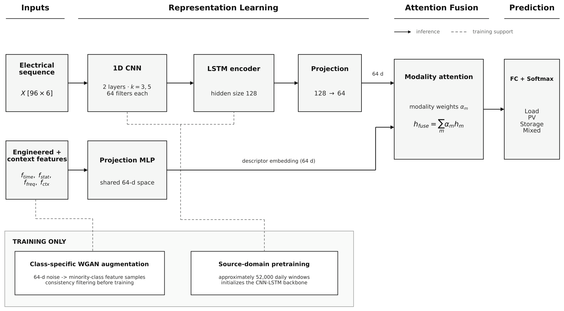
The CNN–LSTM–Attention model comprised three stages. A one-dimensional CNN extracted local patterns from the raw electrical sequence, and an LSTM encoded longer temporal dependencies. The resulting sequence embedding, engineered features, and contextual descriptors were then projected into a shared latent space, where an attention layer combined the complementary representations using learned modality weights.

The feature-extraction and fusion procedure can be written as

$${\mathbf{h}}_{\mathrm{cnn}}=\mathrm{CNN}\left(X\right), {\mathbf{h}}_{\mathrm{lstm}}=\mathrm{LSTM}\left({\mathbf{h}}_{\mathrm{cnn}}\right),$$

(13)

$${\alpha }_m={\displaystyle \frac{\exp \left({\mathbf{q}}^{\top }\tanh \left(W_m{\mathbf{h}}_m\right)\right)}{{\sum }_{k=1}^M\exp \left({\mathbf{q}}^{\top }\tanh \left(W_k{\mathbf{h}}_k\right)\right)}},\hspace{1em}{\mathbf{h}}_{\mathrm{fuse}}={\displaystyle \sum _{m=1}^M}{\alpha }_m{\mathbf{h}}_m,$$

(14)

$$\widehat{y}=\mathrm{Softmax}(W{\mathbf{h}}_{\mathrm{fuse}}+b),$$

(15)

where ${\mathbf{h}}_m$ denotes the encoded representation of modality m, and ${\alpha }_m$ is its learned weight.

Figure 2 summarizes the proposed architecture and its training-only components.

2.6. Evaluation Metrics

Performance was evaluated using accuracy, precision, recall, and F1-score. Because the task contains four classes, overall accuracy was defined as

$$\mathrm{Accuracy}={\displaystyle \frac{1}{N}}{\displaystyle \sum _{i=1}^N}\mathbb{I}({\widehat{y}}_i=y_i),$$

(16)

where N is the number of test samples, and $\mathbb{I}(·)$ is the indicator function. For class c, precision, recall, and F1-score were computed as

$$P_c={\displaystyle \frac{T{P}_c}{T{P}_c+F{P}_c}}, R_c={\displaystyle \frac{T{P}_c}{T{P}_c+F{N}_c}},$$

(17)

$$F{1}_c={\displaystyle \frac{2P_c{R}_c}{P_c+R_c}}.$$

(18)

Macro-recall and macro-F1 give each class equal weight and were calculated as

$$\mathrm{MacroRecall}={\displaystyle \frac{1}{C}}{\displaystyle \sum _{c=1}^C}{R}_c, \mathrm{MacroF}1={\displaystyle \frac{1}{C}}{\displaystyle \sum _{c=1}^C}F{1}_c,$$

(19)

with $C=4$ classes.

3. Case Study and Experimental Setup

3.1. Dataset Description

The case study combined measured transformer-area records with simulation-assisted and WGAN-generated auxiliary samples. The measured dataset was collected from 40 independent low-voltage transformer areas located in multiple regions of Jiangsu Province, including Zhenjiang and Lishui District of Nanjing. The measurement period extended from September 2023 to May 2024. The rated capacities of the distribution transformers ranged from 160 to 630 kVA. Measurements were primarily obtained from existing smart meters and transformer-area data-acquisition terminals and contained aggregated voltage, current, active power, reactive power, power factor, and harmonic-related indicators at 15 min resolution. After data-quality screening, 240 valid daily observation windows, each consisting of 96 time steps, were retained for each transformer area, resulting in a total of 9600 measured or cleaned real windows. Simulation-assisted load, PV, and storage profiles were generated and statistically aligned with the real training data following the procedure described in Section 2.4.

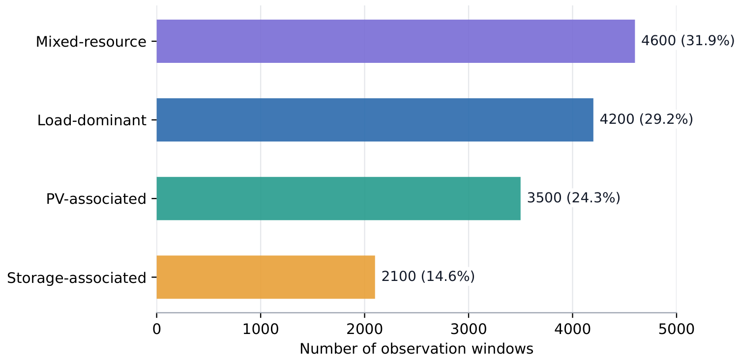
The assembled dataset comprised 14,400 observation windows. Of these, 9600 were measured or cleaned real windows, and 4800 were simulation-assisted or WGAN-generated auxiliary windows. The dataset contained 4200 load-dominant, 3500 PV-associated, 2100 storage-associated, and 4600 mixed-resource windows.

To prevent information leakage across physical sites, the measured data were partitioned at the transformer-area level. Among the 40 independent transformer areas, 22 were assigned to the training subset, 6 to the validation subset, and 12 to the held-out test subset. All observation windows originating from the same physical transformer area were assigned exclusively to one subset. Simulation-assisted and WGAN-generated samples were used exclusively in the training subset, whereas the validation and test subsets contained measured or cleaned real windows only. After the auxiliary samples were incorporated, the nominal dataset allocation followed a 7:1:2 ratio for training, validation, and testing; label-conflict screening was subsequently applied to the real development samples as described in Section 2.3. The held-out test set contained 2880 real observation windows from 12 transformer areas that were not used for model training or validation. The ground-truth labels of all test samples were independently verified using transformer-area equipment installation information, utility asset records, and corresponding operating records. Figure 3 shows the class distribution, and

Table 2. Summary of the pilot case-study dataset.

Item	Description
Observation setting	96 time steps per daily window at 15 min resolution; 240 valid daily windows retained per transformer area after data-quality screening
Input variables	Voltage, current, active power, reactive power, power factor, harmonic-related indicators, and contextual descriptors
Physical dataset	40 independent low-voltage transformer areas in multiple regions of Jiangsu Province, including Zhenjiang and Lishui District of Nanjing; transformer capacities of 160–630 kVA
Data partition	22 training/6 validation/12 held-out test transformer areas; windows from the same physical area were restricted to one subset; auxiliary samples were used only for training
Nominal window allocation	70% training/10% validation/20% testing
Held-out test	2880 measured/cleaned real windows from 12 unseen transformer areas; all labels were independently verified

summarises the dataset.

3.2. Experimental Configuration

All models were implemented in Python 3.10.13, with neural networks developed in PyTorch 2.1.2. Input channels were aligned to a common 15 min time scale, and normalisation statistics were computed exclusively from the training subset. Timing measurements were collected on the same workstation and are therefore interpreted as relative computational costs rather than hardware-independent benchmarks. Comparators included a support vector machine (SVM), random forest (RF), CNN, LSTM, CNN–LSTM–Attention without augmentation, and PatchTST [25] as a recent transformer-based multivariate sequence baseline. The full framework additionally used transfer learning and WGAN-based augmentation.

Table 3. Main hyperparameters of the full model.

Hyperparameter	Value
CNN layers	2 (kernel sizes 3 and 5, 64 filters each)
LSTM hidden size	128
Attention dimension	64
Batch size	64
Learning rate	$1\times {10}^{-3}$ (reduced to $1\times {10}^{-4}$ during fine-tuning)
Optimizer	Adam (${\beta }_1=0.9$, ${\beta }_2=0.999$)
Early stopping patience	10 epochs
WGAN noise dimension	64
WGAN training iterations	5000 per minority class
Transfer learning warm-up	5 epochs (last two layers only)

lists the principal hyperparameters. Training stopped when the validation loss failed to improve for 10 consecutive epochs.

3.3. Evaluation Protocol

Each neural model was trained using five random seeds, and the principal metrics are reported as mean ± standard deviation. For these five repeated runs, 95% confidence intervals were calculated as $\overline{x}\pm t_{0.975,4}s/\sqrt{5}$, where s denotes the sample standard deviation across random seeds. Statistical significance between PatchTST and the proposed method was assessed using a two-sided paired t-test across the five matched random seeds at $\alpha =0.05$. SVM and RF hyperparameters were selected by grid search on the validation subset using the same data split. Supervised model development used only real development windows that passed the conflict-screening procedure in Section 2.3, together with the designated training-only auxiliary samples. Ambiguous real windows were retained for qualitative inspection but excluded from supervised model fitting.

To quantitatively evaluate the distributional fidelity of the WGAN-generated samples, the samples retained after the consistency screening in Section 2.4 were compared with the corresponding real training samples. Before comparison, each feature dimension was standardised using the mean and standard deviation calculated exclusively from the real training subset. For each WGAN-augmented class c and feature dimension j, the 1-Wasserstein distance $W_{1,c,j}$ and the Kolmogorov–Smirnov (KS) statistic $D_{\mathrm{KS},c,j}$ were calculated between the empirical distributions of the real and accepted generated samples. The class-level discrepancies were summarised as

$${\overline{W}}_{1,c}={\displaystyle \frac{1}{d}}{\displaystyle \sum _{j=1}^d}{W}_{1,c,j}, {\overline{D}}_{\mathrm{KS},c}={\displaystyle \frac{1}{d}}{\displaystyle \sum _{j=1}^d}{D}_{\mathrm{KS},c,j},$$

(20)

where d denotes the number of generated feature dimensions. The screening acceptance rate was calculated as

$$R_{\mathrm{acc},c}={\displaystyle \frac{N_{\mathrm{accepted},c}}{N_{\mathrm{generated},c}}}\times 100\%.$$

(21)

Lower Wasserstein distances and KS statistics indicate closer agreement between the generated and real training distributions.

4. Results and Discussion

4.1. Overall Identification Performance

Table 4. Overall performance of the compared methods on the held-out real-only test set.

Method	Input/Training Setting	Accuracy (%)	Macro-Recall (%)	Macro-F1 (%)
SVM	Engineered electrical features	$84.7\pm 0.4$	$82.9\pm 0.6$	$83.2\pm 0.5$
RF	Engineered electrical features	$86.1\pm 0.5$	$84.0\pm 0.5$	$84.9\pm 0.4$
CNN	Single-modal sequence	$89.4\pm 0.6$	$88.0\pm 0.6$	$88.1\pm 0.5$
LSTM	Single-modal sequence	$91.0\pm 0.5$	$89.1\pm 0.6$	$89.6\pm 0.5$
CNN–LSTM–Attention	Multimodal, no augmentation	$92.4\pm 0.4$	$91.0\pm 0.5$	$91.5\pm 0.4$
PatchTST	Multivariate sequence, Transformer	$93.2\pm 0.4$	$92.1\pm 0.5$	$92.6\pm 0.4$
Proposed method	Multimodal + TL + WGAN	$\mathbf{93.8}\pm \mathbf{0.3}$	$\mathbf{93.7}\pm \mathbf{0.4}$	$\mathbf{93.8}\pm \mathbf{0.3}$

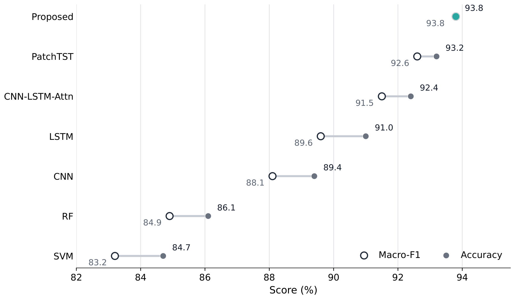
Note: Bold values indicate the best performance among the compared methods.

and Figure 4 compare all models on the held-out real-only test set. PatchTST achieved an accuracy of $93.2\pm 0.4$% and a macro-F1 of $92.6\pm 0.4$%, making it the strongest baseline in terms of mean performance, whereas the proposed method achieved $93.8\pm 0.3$% for both accuracy and macro-F1. The 95% confidence intervals for accuracy were 91.90–92.90% for CNN–LSTM–Attention, 92.70–93.70% for PatchTST, and 93.43–94.17% for the proposed method. These intervals quantify run-to-run uncertainty; the proposed framework retained the highest mean accuracy and macro-F1, with a larger mean margin over PatchTST in macro-F1 than in overall accuracy. A paired comparison across the five matched random seeds yielded a mean accuracy difference of 0.60 percentage points (95% CI: 0.10–1.10 percentage points; $p=0.030$), indicating a statistically significant but modest improvement over PatchTST.

4.2. Effect of Simulation and WGAN Augmentation Under Real-Only Testing

To separately evaluate the contributions of simulation-assisted and WGAN-generated samples, four target-domain training configurations were compared using the same model architecture, source-domain pretraining, data partition, and held-out real-only test set: real data only, real + simulation, real + WGAN, and real + simulation + WGAN. As shown in

Table 5. Effects of simulation-assisted and WGAN-based augmentation under held-out real-only testing.

Training Configuration	Accuracy (%)	Macro-Recall (%)	Macro-F1 (%)
Real only	$91.8\pm 0.5$	$91.1\pm 0.6$	$91.3\pm 0.5$
Real + Simulation	$92.4\pm 0.4$	$91.9\pm 0.5$	$92.0\pm 0.4$
Real + WGAN	$93.1\pm 0.4$	$92.9\pm 0.4$	$93.0\pm 0.4$
Real + Simulation + WGAN	$\mathbf{93.8}\pm \mathbf{0.3}$	$\mathbf{93.7}\pm \mathbf{0.4}$	$\mathbf{93.8}\pm \mathbf{0.3}$

Note: Bold values indicate the best performance among the compared training configurations.

, simulation-assisted training increased the accuracy from 91.8% to 92.4% and the macro-F1 from 91.3% to 92.0%, whereas WGAN augmentation yielded larger gains, reaching 93.1% accuracy and 93.0% macro-F1. Combining both augmentation sources further improved the performance to 93.8% accuracy and 93.8% macro-F1. These results show that both augmentation strategies improved mean performance on real transformer-area data; WGAN yielded the larger individual mean gain under the evaluated configuration, and their combined use achieved the best overall results.

4.3. Distributional Validation of WGAN-Generated Samples

Table 6. Distributional agreement between real and accepted WGAN-generated samples.

Class	Acceptance Rate (%)	Mean ${\mathit{W}}_1$	Mean KS
PV-associated	88.9	0.089	0.076
Storage-associated	85.1	0.106	0.093

reports the distributional agreement between the WGAN-generated samples retained after the class-specific consistency screening and the corresponding real training samples. For the PV-associated class, the screening acceptance rate was 88.9%, with a mean 1-Wasserstein distance of 0.089 and a mean KS statistic of 0.076. For the storage-associated class, the corresponding values were 85.1%, 0.106, and 0.093, respectively. The accepted generated samples therefore showed small class-averaged distributional discrepancies relative to the corresponding real training samples. The slightly larger distances for the storage-associated class are consistent with the greater variability of charging and discharging behaviour.

4.4. Robustness Under Missing Data

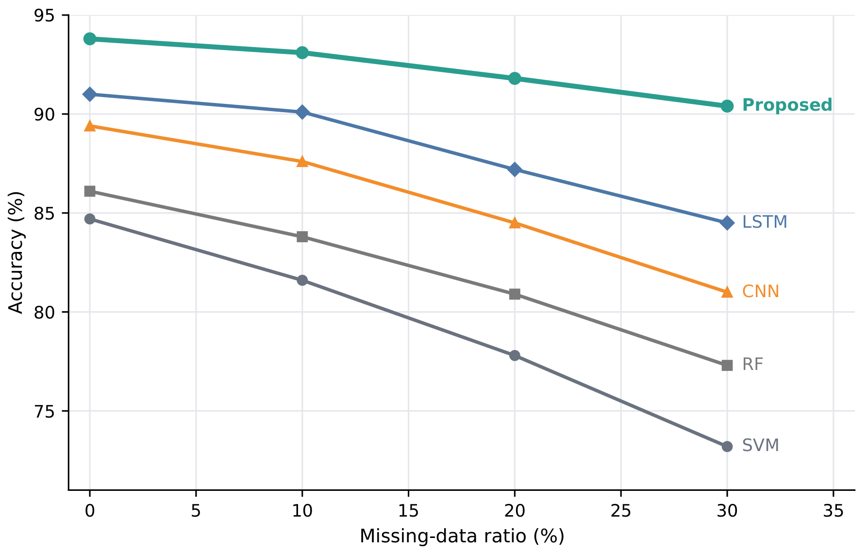
Robustness was first assessed by randomly masking input features and replacing the masked values with zeros at missing ratios of 10%, 20%, and 30%.

Table 7. Accuracy under random missingness and practical field-oriented missing-data patterns.

Panel A. Random Missingness
Missing Ratio	SVM (%)	RF (%)	CNN (%)	LSTM (%)	Proposed (%)
0%	84.7	86.1	89.4	91.0	93.8
10%	81.6	83.8	87.6	90.1	93.1
20%	77.8	80.9	84.5	87.2	91.8
30%	73.2	77.3	81.0	84.5	90.4
Panel B. Practical Missing-Data Patterns
Practical Missing-Data Pattern				Proposed Accuracy (%)
Consecutive missing interval				93.3
Complete channel loss				91.8
Asynchronous measurement				92.8
Communication outage				91.4

and Figure 5 show the resulting accuracy. Performance declined for every model as the missing ratio increased. At 30% missingness, the full framework retained 90.4% accuracy, compared with 84.5% for LSTM and 73.2% for SVM. To further approximate practical field failures, four additional perturbation patterns were evaluated on the held-out real test set. Consecutive missingness was simulated by removing four successive 15 min samples (1 h) from one measurement channel; complete channel loss was evaluated by separately removing each of the six channels over the full 96-step window and averaging the resulting accuracies; asynchronous measurement was simulated by shifting one channel by one sampling interval (15 min); and communication outage was represented by simultaneously removing all six channels for eight consecutive sampling intervals (2 h). Recoverable missing intervals were processed using the same imputation procedure described in Section 2.3. As shown in Table 7, the proposed method retained accuracies of 93.3%, 91.8%, 92.8%, and 91.4% under consecutive missingness, complete channel loss, asynchronous measurement, and communication outage, respectively. The larger degradation under complete channel loss and communication outage indicates that sustained loss of a measurement source or simultaneous multi-channel interruption is more challenging than short recoverable gaps or moderate temporal misalignment.

4.5. Class-Level Identification Behaviour

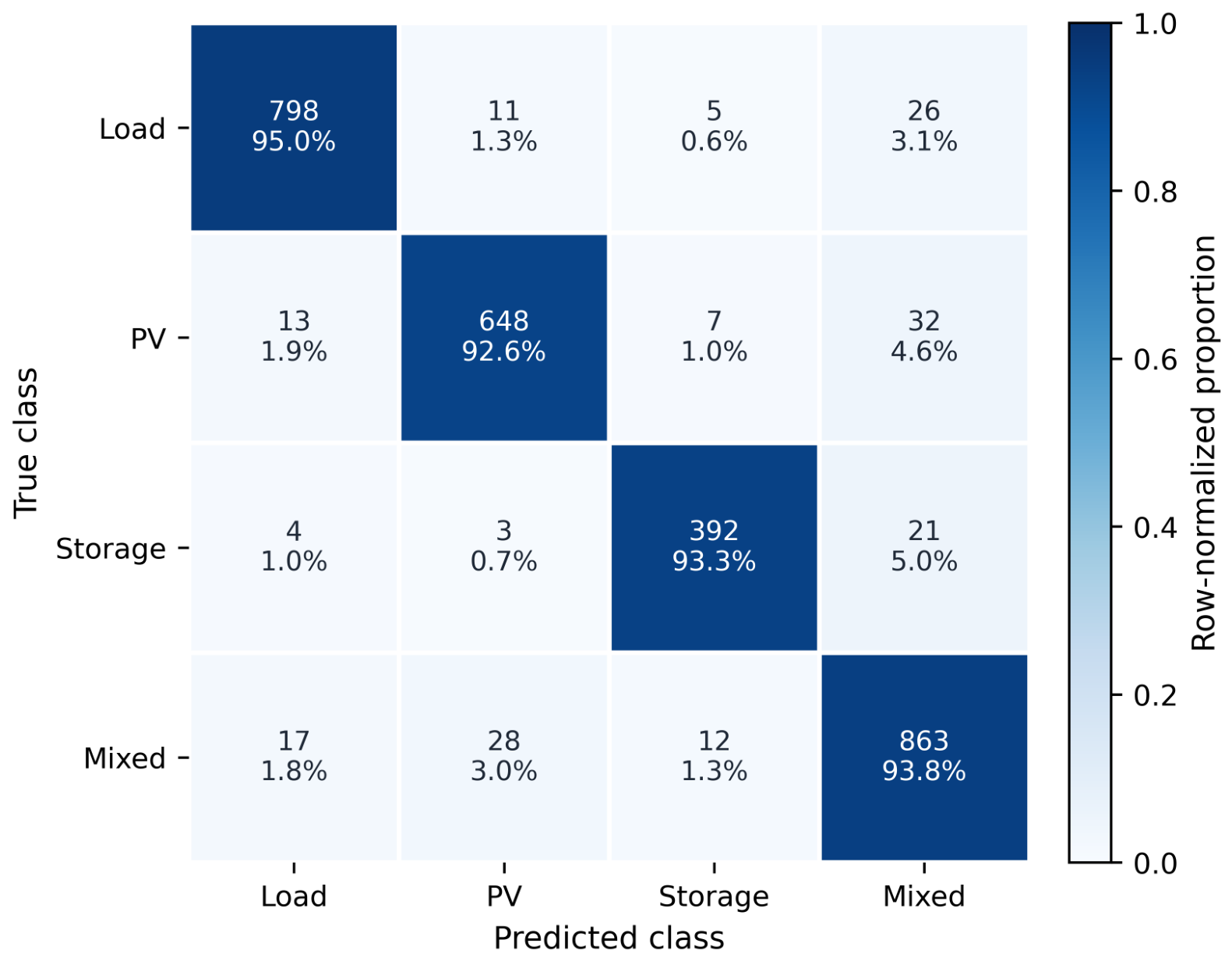
Figure 6 presents the row-normalised confusion matrix for the held-out real-only test set. The set contained 840 load-dominant, 700 PV-associated, 420 storage-associated, and 920 mixed-resource windows. Errors were concentrated between the PV-associated and mixed-resource classes, which share reverse-flow and daytime signatures. Storage-associated windows were also occasionally assigned to the mixed-resource class, reflecting overlap between bidirectional storage operation and flexible-load variation at 15 min resolution.

Table 8. Per-class precision, recall, and F1-score for the proposed framework on the held-out test set.

Class	Precision (%)	Recall (%)	F1 (%)
Load-dominant	95.9	95.0	95.5
PV-associated	93.9	92.6	93.2
Storage-associated	94.2	93.3	93.8
Mixed-resource	91.6	93.8	92.7
Macro-average	93.9	93.7	93.8

reports precision, recall, and F1-score for each class using the same test-set predictions.

4.6. Ablation Study

Table 9. Component ablation results for the proposed framework.

Model Variant	Accuracy (%)	Macro-F1 (%)
Full model	93.8	93.8
w/o transfer learning	92.6	91.7
w/o WGAN augmentation	92.4	92.0
w/o attention fusion	91.7	90.6
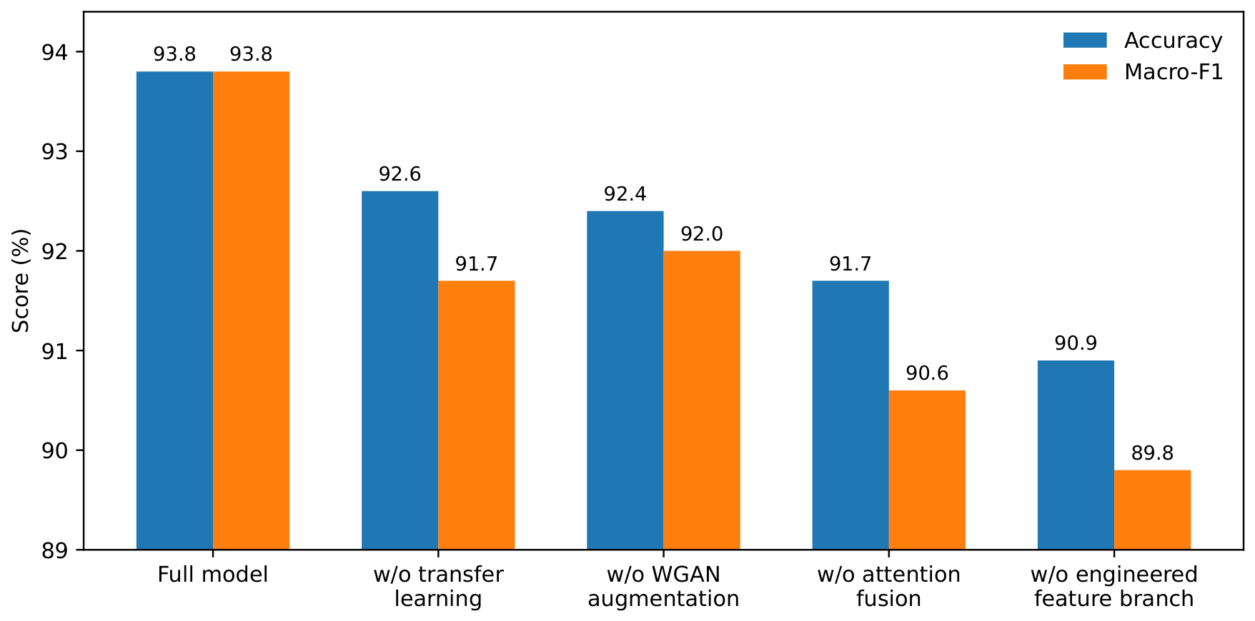
w/o engineered feature branch	90.9	89.8

and Figure 7 report the component ablations. Removing transfer learning or WGAN augmentation reduced accuracy by 1.2 and 1.4 percentage points, respectively. Excluding attention reduced accuracy to 91.7%. The largest decrease occurred without the engineered-feature branch, for which accuracy fell from 93.8% to 90.9%. Within this dataset, the engineered electrical descriptors therefore contributed information that was not fully recovered by the sequence branch alone.

4.7. Computational Efficiency

Table 10. Relative computational cost of selected methods in the pilot environment.

Method	Training Time per Run (min)	Inference Latency per Window (ms)
SVM	0.8	0.12
RF	1.5	0.18
CNN	6.2	0.41
LSTM	7.8	0.57
CNN–LSTM–Attention	8.6	0.63
Proposed method	9.4	0.68

reports wall-clock training time and mean inference latency in the pilot computing environment. The full framework required 9.4 min per training run, compared with 8.6 min for CNN–LSTM–Attention. Mean inference latency was 0.68 ms per window. These measurements indicate modest relative overhead on the test workstation, but they should not be interpreted as hardware-independent deployment benchmarks.

4.8. Engineering Implications and Limitations

The results suggest several potential engineering uses. Resource-pattern estimates could complement existing transformer-area monitoring where measurement density is limited and could help analysts distinguish PV injection, storage response, and mixed-resource behaviour during line-loss or anomaly investigations. The multimodal architecture can also accommodate additional contextual inputs, including weather, feeder topology, and customer metadata; however, the practical value of these extensions remains to be established through deployment studies.

The findings should be interpreted as a pilot validation rather than a broad cross-region or cross-utility benchmark. The training pool partly relied on simulation-assisted data, although testing was restricted to measured or cleaned real windows. Independent utility datasets from multiple regions are therefore needed before operational use. The expert rules in the label library may also require local recalibration when metering practices or network characteristics change.

Although PatchTST was included as a recent transformer-based baseline, broader comparison with additional architectures such as iTransformer [26] remains a direction for future work. Deployment studies should also report platform-specific latency, memory use, update frequency, and secure data-governance procedures. Finally, the remaining confusion between PV-associated and mixed-resource windows indicates a need for more discriminative measurements or hierarchical classification.

5. Conclusions

This study developed a knowledge-guided multimodal learning framework for resource identification from sparse transformer-area measurements. The framework integrates knowledge-guided label screening, multidimensional electrical descriptors, CNN–LSTM–Attention fusion, transfer learning, and WGAN-based augmentation.

On the held-out real-only test set, the framework achieved 93.8% accuracy and a macro-F1 of 93.8%. Under 30% random missingness, accuracy remained at 90.4%. These results support further investigation of multimodal information for transformer-area resource monitoring under the operating conditions represented by the pilot dataset.

Broader conclusions require validation across additional utilities, regions, and measurement regimes. Future work should compare additional recent time-series encoders, quantify predictive uncertainty, and examine topology, weather, and geographical context under realistic deployment constraints.

References

1. Yang, R. Research on User Network Identification Technology for Distribution Transformer Areas. Master’s Thesis, Xi’an University of Technology, Xi’an, China, 2018. [Google Scholar]
2. Wang, S.; Sun, Y.; Zhao, J.; Zheng, S.; Wu, Z.; Shi, C. Comprehensive governance technology for low-voltage distribution networks with large-scale distributed photovoltaics. Electr. Autom. Equip. 2026, 46, 171–179. [Google Scholar] [CrossRef]
3. Men, M.; Zhao, R.; Zhang, J.; Wang, P.; Zhang, Q. Hosting capacity evaluation of distributed photovoltaic in distribution networks based on improved simulated annealing–particle swarm optimization. J. Zhejiang Univ. Eng. Sci. 2024, 58, 1255–1265. [Google Scholar]
4. Goli, P.; Gampa, S.R.; Alluri, A.; Gutta, B.; Jasthi, K.; Das, D. Optimum sizing of solar photovoltaic panels at optimum tilt and azimuth angles using grey wolf optimization algorithm for distribution systems. Inventions 2025, 10, 79. [Google Scholar] [CrossRef] [Scilit]
5. Zhang, X.; Yu, J.; Li, W. Research on supply–demand balance identification in low-voltage transformer areas with high-proportion distributed photovoltaic access. Autom. Appl. 2025, 66, 142–145. [Google Scholar]
6. Zeng, W.; Xiong, J.; Ma, S.; Tan, Y.; Li, J. Control method of distributed energy storage systems for improving photovoltaic accommodation. Energy Storage Sci. Technol. 2022, 11, 3268–3274. [Google Scholar]
7. Brandao, D.A.d.L.; Callegari, J.M.S.; Brandao, D.I.; Pires, I.A. Coordinated, centralized, and simultaneous control of fast charging stations and distributed energy resources. Inventions 2024, 9, 35. [Google Scholar] [CrossRef] [Scilit]
8. Lin, B.; Yang, Z. Abnormal identification of transformer-area line-loss data based on multidimensional features. Power Syst. Prot. Control 2022, 50, 172–178. [Google Scholar]
9. Ren, Y. A Data-Driven Analysis Method for Theoretical Line Loss in Transformer Areas Based on Limited Sample Sets. Master’s Thesis, Shandong University, Jinan, China, 2022. [Google Scholar]
10. Huo, C.; Wang, W.; Yu, K.; Chen, G.; Li, M.; Chen, X.; Dan, T. Prediction of theoretical line loss in transformer areas based on niche genetic algorithm optimized cascade neural networks. Sci. Technol. Eng. 2021, 21, 9897–9906. [Google Scholar]
11. Liubcuk, V.; Radziukynas, V.; Kairaitis, G.; Naujokaitis, D. Power quality impact and its assessment: A review and a survey of Lithuanian industrial companies. Inventions 2025, 10, 30. [Google Scholar] [CrossRef] [Scilit]
12. de Oliveira, F.M.; Brandt, M.H.M.; Salvadori, F.; Izquierdo, J.E.E.; Cavallari, M.R.; Ando Junior, O.H. Development of an MPPT-based genetic algorithm for photovoltaic systems versus classical MPPT techniques in scenarios with partial shading. Inventions 2024, 9, 64. [Google Scholar] [CrossRef] [Scilit]
13. Zhao, Y.; Qin, W.; Wei, H.; Pan, X.; Xu, J. Availability analysis and assurance of wireless public network communication in distribution automation. Distrib. Util. 2014, 31, 43–48. [Google Scholar]
14. Karimov, J.; Rabl, T.; Katsifodimos, A.; Samarev, R.; Heiskanen, H.; Markl, V. Benchmarking distributed stream data processing systems. In Proceedings of the 2018 IEEE 34th International Conference on Data Engineering, Paris, France, 16–19 April 2018; pp. 1507–1518. [Google Scholar]
15. Li, G.; Hung, C.C.; Liu, M.; Pan, L.; Peng, W.-C.; Chan, S.H.G. Spatial-temporal similarity for trajectories with location noise and sporadic sampling. In Proceedings of the 2021 IEEE 37th International Conference on Data Engineering, Chania, Greece, 19–22 April 2021; pp. 1224–1235. [Google Scholar]
16. Chen, B.; Li, Q.; Ma, R.; Qian, X.; Wang, X.; Li, X. Towards the generalization of time series classification: A feature-level style transfer and multi-source transfer learning perspective. Knowl.-Based Syst. 2024, 299, 112057. [Google Scholar] [CrossRef] [Scilit]
17. Liu, K.; Zhou, F.; Zhou, H.; Wang, C. Repair of transformer-area acquisition data based on improved generative adversarial networks. Power Syst. Technol. 2022, 46, 3231–3240. [Google Scholar]
18. Huang, Z. Cross-regional investment benefit prediction model for distribution networks based on transfer learning. Rural Electrif. 2025, 35–38. [Google Scholar] [CrossRef]
19. Zhai, S.; Liang, J.; Yang, W.; Zheng, C.; Wang, D.; Xing, X.; Feng, Y. Weakly supervised optimization for power distribution transformer area identification based on frequency-domain representation. Electronics 2026, 15, 1000. [Google Scholar] [CrossRef] [Scilit]
20. Lv, J.; Zhang, N.; Xie, Y.; Liu, H. Low-voltage distribution network topology identification based on feature selection and multi-feature decision-making. Electr. Eng. 2025, 107, 12961–12978. [Google Scholar] [CrossRef] [Scilit]
21. Jiang, Y.; Chen, T.; Yuan, J.; Zhao, M.; Liu, Y. A robust topology identification method of distribution network based on counterfactual samples and generative adversarial networks. J. Supercomput. 2025, 81, 1372. [Google Scholar] [CrossRef] [Scilit]
22. Cai, Y.; Wen, Y.; Zhang, Z.; Xu, Y.; Li, X.; Zhao, C. Typical scenario division method for low-voltage transformer areas based on resource endowment and load characteristics. Power Big Data 2024, 27, 19–26. [Google Scholar]
23. Zhu, X.; Peng, B.; Si, Y.; Wu, J.; Lou, J.; Xi, Y. Comprehensive evaluation of distribution networks based on knowledge graph. Mod. Electr. Power 2022, 39, 677–684. [Google Scholar]
24. Trindade, A. ElectricityLoadDiagrams20112014. UCI Machine Learning Repository. 2015. Available online: https://archive.ics.uci.edu/dataset/321/electricityloaddiagrams20112014 (accessed on 13 September 2026).
25. Nie, Y.; Nguyen, N.H.; Sinthong, P.; Kalagnanam, J. A Time Series Is Worth 64 Words: Long-Term Forecasting with Transformers. In Proceedings of the Eleventh International Conference on Learning Representations (ICLR), Kigali, Rwanda, 1–5 May 2023; OpenReview.net: Amherst, MA, USA, 2023. [Google Scholar]
26. Liu, Y.; Hu, T.; Zhang, H.; Wu, H.; Wang, S.; Ma, L.; Long, M. iTransformer: Inverted Transformers Are Effective for Time Series Forecasting. In Proceedings of the Twelfth International Conference on Learning Representations (ICLR), Vienna, Austria, 7–11 May 2024; OpenReview.net: Amherst, MA, USA, 2024. [Google Scholar]
Figure 1. Multidimensional feature-construction workflow for transformer-area measurements.
Information 17 00904 g001
Figure 2. Architecture of the proposed multimodal CNN–LSTM–Attention framework, including training-only WGAN augmentation and source-domain pretraining.
Information 17 00904 g002
Figure 3. Class distribution of the 14,400-window pilot case-study dataset.
Information 17 00904 g003
Figure 4. Accuracy and macro-F1 comparison on the held-out real-only test set. The proposed method is highlighted in teal.
Information 17 00904 g004
Figure 5. Accuracy under increasing random missing-data ratios.
Information 17 00904 g005
Figure 6. Row-normalised confusion matrix for the proposed framework on the held-out real-only test set; each cell also reports the corresponding sample count.
Information 17 00904 g006
Figure 7. Accuracy and macro-F1 under component ablations of the proposed framework.
Information 17 00904 g007