LG-MACFM: Local Gaussian Process Prior-Guided Mask-Aware Conditional Flow Matching for Renewable Energy Imputation

Abstract

Renewable energy generation data usually exhibit strong spatial correlations and temporal continuity, but measurement curves from wind and photovoltaic stations often contain sporadic missing entries and continuous missing segments due to communication interruptions, device failures, and abnormal monitoring. Existing spatio-temporal imputation methods commonly rely on deterministic reconstruction or generative processes initialized from standard Gaussian noise, which limits their ability to exploit local spatio-temporal structures in the observed data. To address this problem, we propose a local Gaussian process (GP) prior-guided mask-aware conditional flow matching framework for renewable energy imputation (LG-MACFM). Connected missing positions are grouped into bounded blocks, and a local set of relevant observations is used to construct a joint GP-informed source prior for each block, replacing the conventional isotropic Gaussian source distribution. The source-prior mean and covariance provide a structured initial state for the flow. Based on this prior, a spatio-temporal network-guided mask-aware conditional flow matching module transports GP-informed samples toward the target data distribution while strictly preserving the observed entries throughout the continuous generation path. Covariance-aware endpoint supervision accounts for source-prior uncertainty, while relation matching preserves target spatio-temporal differences. During inference, missing values are generated by solving a mask-aware ordinary differential equation (ODE) from the GP-informed initial state. Experimental results demonstrate that the proposed method achieves more accurate and structurally consistent imputation results than existing baselines.

1. Introduction

With the rapid integration of renewable energy into modern power systems, accurate monitoring of wind and photovoltaic generation has become increasingly critical for system operation, energy management, and grid stability. Renewable generation data often exhibit strong spatial correlations among geographically related stations and temporal continuity within short-term measurement curves because nearby generation nodes are commonly influenced by similar meteorological and environmental factors. These spatio-temporal characteristics provide important information for capturing generation patterns and supporting reliable data-driven analysis. Therefore, complete and high-quality measurement records are essential for downstream applications, including power forecasting, anomaly detection, dispatch optimization, and operational risk assessment [1,2,3,4].

In practical monitoring environments, renewable energy generation curves are often corrupted by missing values. Communication failures, sensor malfunctions, equipment faults, abnormal monitoring states, and transmission errors can cause random missing entries in wind and photovoltaic station data [5]. These missing values are usually irregularly distributed across both spatial and temporal dimensions [6], making imputation more difficult than simple interpolation or short-gap recovery. Inaccurate reconstruction of such corrupted data may further impair the reliability of subsequent forecasting, control, and decision-making models [7,8,9].

Early imputation methods relied on interpolation, k-nearest neighbors (KNN), and low-rank reconstruction [9,10,11]. Although computationally efficient, these methods are governed by fixed local or linear assumptions and have limited ability to represent the nonlinear variations of renewable generation. Data-driven methods subsequently introduced context encoders, convolutional reconstruction, and attention mechanisms for wind and photovoltaic measurements [12,13,14]. These models learn temporal and cross-variable patterns more flexibly, but their point-estimation objectives do not characterize the uncertainty associated with missing values. Graph-based models further exploit the dependence among geographically related sensors. GRIN and SPIN propagate temporal information over sensor graphs and improve reconstruction from sparse observations [15,16], while STAMImputer incorporates dynamically sampled graph attention for blockwise traffic-data missingness [17]. Such methods demonstrate the value of explicit spatial modeling, but they predominantly produce a single reconstruction. Probabilistic models provide an alternative by learning latent distributions or progressively generating conditional samples. Gaussian process (GP) priors introduce temporal structure into latent-variable models such as GP-VAE [18], whereas CSDI, PriSTI, and CoFILL use diffusion processes with temporal or spatio-temporal conditioning [19,20,21]. However, diffusion-based imputers commonly start from data-independent Gaussian noise, which limits their ability to fully exploit the observed spatio-temporal dependencies.

Flow matching provides a continuous-time alternative that can transport samples from flexible source distributions to the target distribution [22,23]. For instance, Impute-MACFM restricts conditional transport to missing entries in tabular data [24]. TSFlow incorporates GP priors for probabilistic time-series forecasting [25]. GiFlow constructs graph-informed source states for spatio-temporal imputation [26]. These developments establish the feasibility of mask-aware transport and observation-informed initialization, but two issues remain in probabilistic renewable energy imputation. First, when generation begins from independent noise or independently constructed source states, the source distribution does not sufficiently reflect the observed spatio-temporal information or represent the dependencies among connected missing positions. The generative model must then recover this structure during transport, although relevant observations are already available around the missing region. Second, pointwise supervision is inadequate for structured missing regions because errors at connected positions are generally correlated, and similar pointwise errors may correspond to different temporal changes or spatial contrasts. Treating these positions independently therefore overlooks both block-level uncertainty and the internal relations of the target pattern.

To address these issues, we propose a local Gaussian process prior-guided mask-aware conditional flow matching framework (LG-MACFM). Locality is imposed by partitioning connected missing positions into bounded blocks and selecting a block-specific top-K set of relevant observations. LG-MACFM uses this local context to construct a joint GP-informed source prior for each block. A spatio-temporal velocity network then transports samples only at missing positions while retaining the observations as fixed conditions. Covariance-aware endpoint supervision and relation matching further account for block-level uncertainty and internal spatio-temporal relations, respectively.

The main contributions are summarized as follows:

• We formulate renewable energy imputation as conditional transport from a local joint GP-informed source prior for each missing block, which is constructed from relevant observations and captures dependence among connected missing positions.
• We design a spatio-temporal velocity network to capture graph-based spatial dependencies and temporal dynamics. Combined with mask-aware conditional flow matching, it updates only missing positions while keeping observations fixed.
• We introduce covariance-aware endpoint and relation-matching objectives that respectively weight joint endpoint errors using the source-prior covariance and align predicted spatio-temporal differences with their targets.

2. Related Work

2.1. Predictive Methods for Time-Series Imputation

Predictive methods estimate a single value for each unobserved entry. They can be grouped according to their modeling mechanisms. Early methods were primarily statistical or similarity-based. Soft-Impute completes a low-rank matrix [11], MICE alternates conditional regressions across variables [10], and MissForest replaces these regressions with random forests [27]. ST-MVL instead combines several temporal and spatial views for sensor-data estimation [28]. These approaches are computationally accessible, but their accuracy depends on low-rank, conditional-model, or local-smoothness assumptions. They also struggle with strongly nonlinear and nonstationary dependencies.

Recurrent neural network (RNN)- and convolutional neural network (CNN)-based methods learn nonlinear temporal patterns directly from incomplete sequences. GRU-D uses trainable decay factors to represent elapsed time and informative missingness [29]. BRITS estimates missing values in both temporal directions and enforces consistency between the two estimates [30]. M-RNN combines interpolation with multi-directional recurrent estimates across time and variables [31]. The sequential nature of recurrent processing can cause errors to accumulate across long gaps and restrict parallel computation. Convolutional alternatives improve efficiency, but their local receptive fields may miss long-range dependencies.

Attention-based methods expand the temporal receptive field and model interactions among variables. DeepMVI combines convolutional features with attention across correlated series [32]. SAITS stacks diagonally masked self-attention blocks and adaptively combines their estimates [33]. ImputeFormer introduces low-rank temporal and spatial attention for high-dimensional spatio-temporal data [34]. TIDER couples interpolation and denoising tasks through a Transformer architecture [35]. These methods capture long-range dependencies, but self-attention can become costly for long, high-dimensional sequences. Their estimates also deteriorate when little informative context remains around a gap.

Graph neural network (GNN)-based methods explicitly encode relations among sensors or variables. GRIN performs bidirectional recurrent message passing on a sensor graph [15]. SPIN uses spatio-temporal graph attention without recursively feeding previous imputations into later estimates [16]. Casper introduces causality-aware graph representations to suppress spurious dependencies [36]. STAMImputer combines dynamically sampled graph attention with a mixture-of-experts design [17]. Their performance depends on graph quality. Incorrect edges or changing topology can propagate misleading information, whereas few observed neighbors limit the evidence available for aggregation.

2.2. Generative Methods for Time-Series Imputation

Generative methods model a conditional distribution over missing entries and can produce multiple plausible completions. Variational autoencoder (VAE)- and generative adversarial network (GAN)-based methods form one major group. GAIN uses an adversarial discriminator and a hint mechanism to identify observed and imputed components [37]. E²GAN combines recurrent encoding and decoding with adversarial learning for multivariate sequences [38]. SSGAN adds semi-supervised signals to adversarial imputation [39], whereas GP-VAE places a Gaussian process prior in the latent space [18]. BayOTIDE uses Bayesian functional decomposition [40], and TimeCIB learns conditional representations through an information bottleneck [41]. VAE-based models remain sensitive to their prior assumptions, and GAN training can be unstable and is susceptible to mode collapse.

Diffusion-based methods generate conditional samples by progressively reversing a prescribed noising process. CSDI learns a conditional score model for the missing entries [19]. SSSD introduces a structured state-space backbone [42], while MIDM enforces consistency at observed positions [43]. PriSTI incorporates spatio-temporal conditioning [20], and MTSCI adds temporal-consistency constraints [44]. NewImp analyzes imputation through gradient flow [45], whereas CoFILL combines conditional diffusion with temporal and frequency information [21]. Diffusion models can represent flexible conditional distributions, but inference usually requires many reverse denoising steps. Their performance is also sensitive to the noise schedule, denoiser capacity, and conditioning quality.

Flow matching-based methods learn a continuous velocity field that transports samples from a source distribution to the data distribution [22,23]. Impute-MACFM learns mask-aware conditional trajectories for tabular imputation [24]. TSFlow constructs Gaussian process source distributions for probabilistic forecasting [25]. GiFlow uses graph-informed source states for spatio-temporal imputation [26]. These methods learn transport directly without requiring iterative reverse denoising, but accurate velocity-field learning remains difficult. Performance also depends on the source distribution and transport path. Existing formulations do not jointly construct a locally conditioned source distribution that preserves correlations among missing positions and supports mask-aware transport for continuous missing segments.

2.3. Renewable Energy Data Imputation

Renewable energy data require dedicated treatment because power and meteorological signals vary rapidly and are correlated across sites and variables. Conventional studies usually treat recovery as a preprocessing step and compare interpolation, KNN, MICE, or Soft-Impute [9,10,11]. CPI instead retrieves comparable historical segments and preserves the energy of each reconstructed gap [46]. Such approaches are simple and interpretable, but sufficiently similar historical segments may not exist under changing operating conditions. Their deterministic reconstructions are also vulnerable to regime shifts and extended gaps.

Application-specific neural models incorporate operational context into the reconstruction process. CE uses an encoder–decoder–discriminator architecture to reconstruct wind-farm measurements [12]. SRPCNN reconstructs random and continuous gaps before IBLS performs online-updatable solar forecasting [13]. Rec-LSTM integrates recurrent missing-input recovery with probabilistic photovoltaic forecasting [47]. Other studies use spatio-temporal and cross-feature correlations [48], constrained encoder–decoder architectures [49], or attention-based two-stage learning [14]. These designs demonstrate several ways of incorporating domain information into reconstruction.

However, their performance and applicability often depend on specific signals, sites, forecasting pipelines, and missingness patterns. Broad evaluations confirm that imputer rankings vary with both the signal type and the missingness pattern [7]. Moreover, most methods focus on pointwise reconstruction and do not explicitly model joint uncertainty among correlated missing positions.

The related work is summarized in

Table 1. Evolution and comparison of representative time-series imputation methods.

Paradigm	Category	Representative Model	Core Mechanism	Representative Limitation
Predictive	Statistical and similarity-based	Soft-Impute (2010) [11]; MICE (2011) [10]; MissForest (2012) [27]; ST-MVL (2016) [28]; CPI (2021) [46]	Soft-Impute estimates a low-rank matrix; MICE alternates conditional regressions across variables; MissForest replaces them with random forests; ST-MVL fuses multiple spatio-temporal views; CPI copies a comparable historical segment while preserving gap energy.	Performance depends on low-rank, conditional-model, local-smoothness, or recurring-pattern assumptions. These methods have limited capacity for nonlinear, nonstationary dynamics and commonly return a single deterministic completion.
	RNN/ CNN-based	GRU-D (2018) [29]; BRITS (2018) [30]; M-RNN (2019) [31]; SRPCNN–IBLS (2022) [13]; Rec-LSTM (2022) [47]	GRU-D learns decay factors for stale observations; BRITS combines forward and backward recurrent imputations with a consistency loss; M-RNN uses multi-directional recurrent estimates; SRPCNN–IBLS pairs convolutional reconstruction with online solar forecasting; Rec-LSTM integrates recursive imputation with probabilistic photovoltaic forecasting.	RNN-based models can accumulate errors over long gaps and may be costly for long sequences. CNN components are constrained by local receptive fields, and most methods in this family provide point estimates rather than calibrated predictive distributions.
	Attention-based	DeepMVI (2021) [32]; SAITS (2023) [33]; TIDER (2023) [35]; ImputeFormer (2024) [34]	DeepMVI combines convolutional features with attention across variables; SAITS uses two diagonally masked self-attention blocks and combines their estimates; TIDER couples interpolation and denoising tasks; ImputeFormer introduces a low-rank inductive bias into Transformer-based spatio-temporal imputation.	Self-attention becomes memory- and compute-intensive as sequence length and dimensionality grow. Reconstruction also depends on informative observed context.
	GNN-based	GRIN (2022) [15]; SPIN (2022) [16]; Casper (2024) [36]; STAMImputer (2025) [17]	GRIN performs bidirectional recurrent message passing on a sensor graph; SPIN reconstructs sparse observations with spatio-temporal graph attention; Casper learns causality-aware graph representations to suppress spurious dependencies; STAMImputer combines spatio-temporal attention with a mixture-of-experts design.	Results depend on the quality and stationarity of the prescribed graph. Imperfect edges and over-smoothing can distort propagation, and large missing blocks leave few observed messages for graph-based aggregation.
Generative	VAE/GAN-based	GAIN (2018) [37]; E2GAN (2019) [38]; GP-VAE (2020) [18]; SSGAN (2021) [39]; CE (2022) [12]; BayOTIDE (2023) [40]; TimeCIB (2024) [41]	GAIN uses a hint mechanism and discriminator; E2GAN combines an encoder–decoder with adversarial training; GP-VAE uses a temporal Gaussian process latent prior; SSGAN adds semi-supervised adversarial learning; CE applies context encoding to wind-farm reconstruction; BayOTIDE uses Bayesian functional decomposition; TimeCIB learns conditional representations through an information bottleneck.	Adversarial objectives can be unstable and may suffer from mode collapse. Latent-variable and functional priors also require careful specification, and uncertainty represented by generated samples is not necessarily calibrated.
	Diffusion-based	CSDI (2021) [19]; SSSD (2022) [42]; MIDM (2023) [43]; PriSTI (2023) [20]; MTSCI (2024) [44]; NewImp (2024) [45]; CoFILL (2025) [21]	CSDI learns a conditional score network for missing entries; SSSD incorporates structured state-space sequence modeling; MIDM imposes observed-value consistency; PriSTI conditions diffusion on spatio-temporal structure; MTSCI introduces temporal-consistency constraints; NewImp studies imputation from a gradient-flow perspective; CoFILL applies conditional diffusion to spatio-temporal data.	Sampling requires many reverse denoising steps and is therefore expensive for long or high-dimensional sequences. Performance is sensitive to the noise schedule, denoiser capacity, and fidelity of the conditioning information.
	Flow matching-based	Impute-MACFM (2025) [24]; TSFlow (2025) [25]; GiFlow (2026) [26]	Impute-MACFM learns mask-aware conditional trajectories for tabular gaps; TSFlow constructs Gaussian process source priors for probabilistic forecasting; GiFlow uses graph-informed flow matching for spatio-temporal imputation.	Flow-based imputation depends on accurate velocity-field learning and on the choice of source distribution and transport path. Existing formulations do not jointly construct a local probabilistic source with correlated initialization and mask-aware transport for continuous missing segments.

. The table distinguishes predictive methods from generative methods and compares the principal architectural categories by their representative models, core mechanisms, and inherent limitations. Overall, the comparison shows a progression from deterministic reconstruction toward probabilistic generation. It also highlights unresolved challenges in modeling dependencies among missing values, efficient conditional generation, and robust recovery of continuous missing segments.

3. Preliminaries

3.1. Problem Formulation

The renewable energy generation system is represented as a spatial graph $\mathcal{G}=(\mathcal{V},\mathcal{E},\mathbf{A})$, where $\mathcal{V}$ is the set of N generation nodes, $\mathcal{E}$ is the set of spatial connections, and $\mathbf{A}$ is the geographical adjacency matrix.

The original generation measurement curves are denoted by $\mathbf{Y}\in {\mathbb{R}}^{N\times T}$, where $Y_{i,\tau }$ represents the generation value of node i at time index $\tau$. The whole sequence is divided into fixed-length temporal windows. For the b-th window, the corresponding complete data segment is denoted by ${\mathbf{X}}_1^{\left(b\right)}\in {\mathbb{R}}^{N\times L}$, where L is the window length. The subscript 1 indicates that this complete window serves as the data endpoint in the flow matching process. For simplicity, the superscript b is omitted when there is no ambiguity.

Each window is associated with a binary mask $\mathbf{M}\in {\{0,1\}}^{N\times L}$, where $M_{i,\tau }=1$ and $M_{i,\tau }=0$ indicate observed and missing positions, respectively. These positions form the condition set $\mathcal{C}$ and target set $\mathcal{T}$. We represent the observed tensor as ${\mathbf{X}}_{\mathcal{C}}=\mathbf{M}\odot {\mathbf{X}}_1$ and denote the missing target values by ${\mathbf{X}}_{\mathcal{T}}$. The task is to model the conditional distribution of ${\mathbf{X}}_{\mathcal{T}}$ given ${\mathbf{X}}_{\mathcal{C}}$, $\mathbf{M}$, and $\mathbf{A}$ while preserving the observed entries. The main notation is summarized in

Table 2. Summary of the main notation.

Notation	Description
$\mathcal{G}$	Spatial graph of renewable energy generation nodes
$\mathcal{V}$	Set of renewable energy generation nodes
$\mathcal{E}$	Set of spatial connections among nodes
$\mathbf{A}$	Adjacency matrix describing geographical dependencies
N	Number of renewable energy generation nodes
T	Total number of time steps
L	Length of each temporal window
$\mathbf{Y}$	Original renewable energy generation measurement curves
$\tau$	Discrete time index in the temporal window
${\mathbf{X}}_1$	Complete data window used as the flow endpoint
$\mathbf{M}$	Binary observation mask
$M_{i,\tau }=1$	Observed (conditioning) entry
$M_{i,\tau }=0$	Missing (target) entry
$\mathcal{C}$	Condition index set of observed spatio-temporal positions
$\mathcal{T}$	Target index set of missing spatio-temporal positions
${\mathbf{X}}_{\mathcal{C}}$	Observed tensor $\mathbf{M}\odot {\mathbf{X}}_1$
${\mathbf{X}}_{\mathcal{T}}$	Target generation values to be imputed
t	Continuous flow time in the generative process
$\theta$	Learnable model parameters

.

3.2. Conditional Flow Matching

Conditional flow matching (CFM) [22,23] learns a time-dependent velocity field that transports samples from a source distribution $q_0$ to a target distribution $q_1$. Given paired samples ${\mathbf{x}}_0\sim q_0$ and ${\mathbf{x}}_1\sim q_1$ and a flow time $t\sim \mathcal{U}(0,1)$, we use the deterministic linear path and its conditional velocity:

$${\mathbf{x}}_t=(1-t){\mathbf{x}}_0+t{\mathbf{x}}_1,{\mathbf{u}}_t={\mathbf{x}}_1-{\mathbf{x}}_0,$$

(1)

where ${\mathbf{x}}_t$ is the intermediate state and ${\mathbf{u}}_t$ is the target velocity. For conditional generation, a neural velocity field ${\mathbf{v}}_{\theta }(t,{\mathbf{x}}_t,\mathbf{c})$ additionally receives the condition $\mathbf{c}$ and is optimized by

$${\mathcal{L}}_{\mathrm{CFM}}\left(\theta \right)={\mathbb{E}}_{t,{\mathbf{x}}_0,{\mathbf{x}}_1}\left[{∥{\mathbf{v}}_{\theta }(t,{\mathbf{x}}_t,\mathbf{c})-{\mathbf{u}}_t∥}_2^2\right],$$

(2)

where $\mathbf{c}$ denotes the auxiliary condition and $\theta$ denotes the learnable parameters. After training, samples are generated by integrating the learned ODE:

$${\displaystyle \frac{d{\mathbf{x}}_t}{dt}}={\mathbf{v}}_{\theta }(t,{\mathbf{x}}_t,\mathbf{c}),{\mathbf{x}}_0\sim q_0.$$

(3)

Therefore, CFM learns a continuous transport from the source distribution to the target distribution by directly regressing the conditional velocity field, while allowing the source distribution to be specified according to the task.

4. Methodology

4.1. Overall Framework

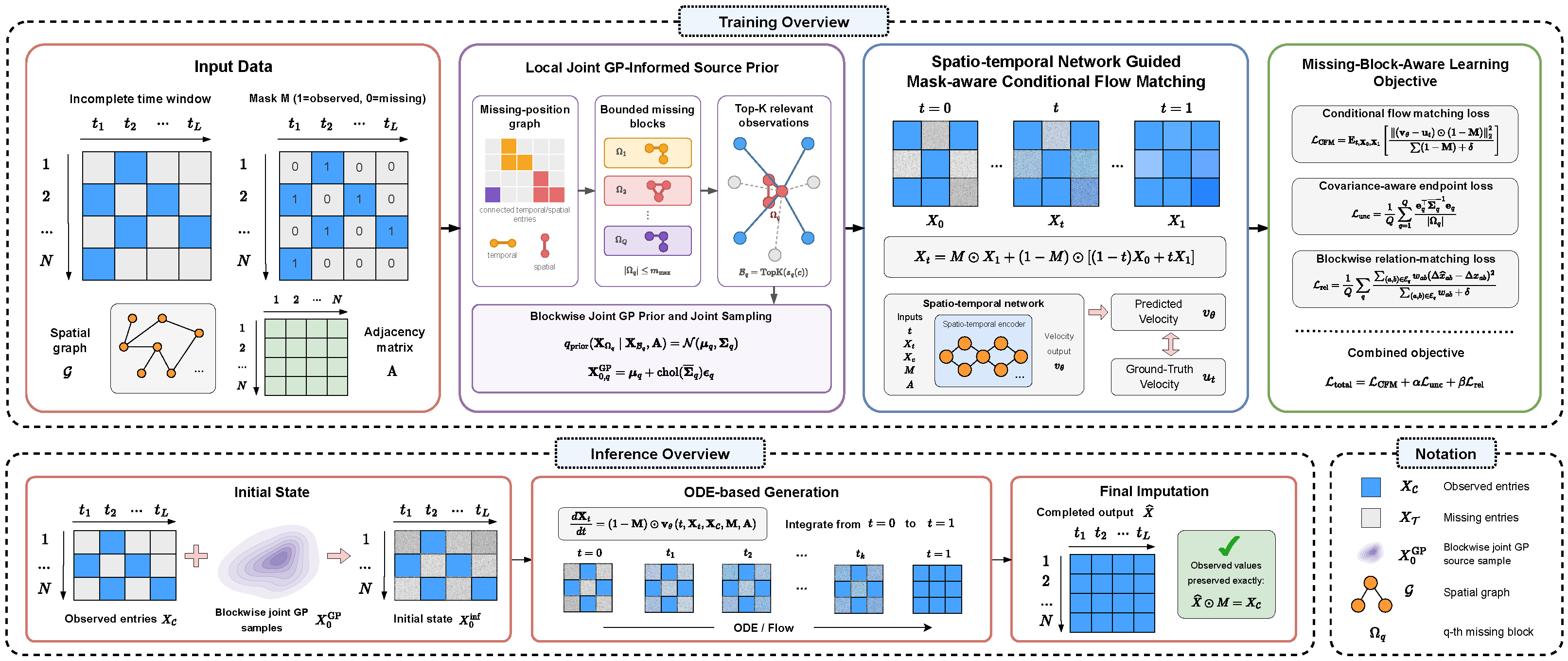
Given the observed entries ${\mathbf{X}}_{\mathcal{C}}$, the mask matrix $\mathbf{M}$, and the geographical structure $\mathbf{A}$, our goal is to generate the missing target entries ${\mathbf{X}}_{\mathcal{T}}$. Unlike conventional flow matching-based imputation methods that start from an unstructured Gaussian distribution, we construct a local joint spatio-temporal GP source prior for each missing block. To retain the dependencies induced by the observed spatio-temporal signals, the GP source prior is constructed jointly over the connected missing positions within each block rather than factorized over individual positions.

As shown in Figure 1, the proposed method consists of three main components. First, a missing-position graph groups temporally or spatially connected missing entries into blocks, and a shared top-K observation set is used to construct a local joint GP-informed source prior for each block. Second, a spatio-temporal network-guided mask-aware conditional flow matching process transports samples from the GP-informed prior distribution to the target data distribution while strictly preserving the observed entries. Third, a covariance-aware endpoint loss and a blockwise relation-matching loss incorporate joint uncertainty and preserve the intrinsic spatio-temporal relationships in the target data.

After training, the learned velocity field is used in the inference stage to solve a mask-aware ODE from the GP-informed initial state, generating the missing entries while preserving the observed values.

4.2. Local Joint GP-Informed Prior for Missing Blocks

The initial distribution of the flow plays an important role in conditional generation. For spatio-temporal imputation, sampling the missing entries from an unstructured standard Gaussian distribution ignores the strong correlations among renewable generation nodes and their temporal contexts. To provide a more informative starting point for the generative process, we construct a local joint GP-informed source prior for each missing block. Here, local refers to the bounded scope of each source prior. It is constructed for one missing block from a block-specific top-K set of relevant observations rather than from the complete spatio-temporal window, while the missing positions within that block are modeled jointly through a full covariance matrix.

A spatio-temporal position is denoted by $r=(i,\tau )$, where i and $\tau$ represent the node index and temporal index, respectively. For two positions $r=(i,\tau )$ and $r^{\prime }=(j,s)$, we define a separable spatio-temporal kernel as follows:

$$k(r,r^{\prime })={\sigma }_f^2{k}_s(i,j)k_t(\tau ,s),$$

(4)

where ${\sigma }_f^2$ is the signal variance, $k_s(i,j)$ denotes the spatial kernel, and $k_t(\tau ,s)$ denotes the temporal kernel.

The spatial kernel is defined through graph diffusion on the geographical adjacency matrix $\mathbf{A}$. Let $\tilde{\mathbf{A}}=\mathbf{A}+\mathbf{I}$ denote the adjacency matrix with self-loops, and let $\tilde{\mathbf{D}}$ be its degree matrix. The normalized graph Laplacian is given by

$${\mathbf{L}}_s=\mathbf{I}-{\tilde{\mathbf{D}}}^{-{\displaystyle \frac{1}{2}}}\tilde{\mathbf{A}}{\tilde{\mathbf{D}}}^{-{\displaystyle \frac{1}{2}}}.$$

(5)

The spatial kernel is then defined as

$$k_s(i,j)={\displaystyle \frac{{\left[exp(-\gamma {\mathbf{L}}_s)\right]}_{ij}}{\sqrt{{\left[exp(-\gamma {\mathbf{L}}_s)\right]}_{ii}{\left[exp(-\gamma {\mathbf{L}}_s)\right]}_{jj}}}},$$

(6)

where $\gamma >0$ controls the spatial diffusion range and $k_s(i,j)$ represents the spatial similarity between nodes i and j.

The temporal kernel characterizes local temporal dependencies within each window. Since renewable generation values usually evolve smoothly over short time intervals, we adopt a squared exponential kernel:

$$k_t(\tau ,s)=exp\left(-{\displaystyle \frac{{(\tau -s)}^2}{2{\ell }_t^2}}\right),$$

(7)

where ${\ell }_t$ is the temporal length scale controlling the correlation range along the time dimension.

The mask induces a missing-position graph, whose temporal edges connect consecutive missing positions at the same node and whose spatial edges connect simultaneous missing positions at adjacent nodes. Its connected components are used to form the missing blocks. To prevent a large component from producing a costly GP covariance matrix, we impose a maximum block size $m_{max}$. If a component exceeds this limit, repeated breadth-first searches partition it along the temporal and spatial edges into connected sub-blocks of at most $m_{max}$ positions. The resulting blocks form a disjoint partition of the missing set:

$${\mathcal{G}}_{\mathrm{mis}}=(\mathcal{T},{\mathcal{E}}_t\cup {\mathcal{E}}_s),\mathcal{T}={\displaystyle \underset{q=1}{\overset{Q}{⨆}}}{\Omega }_q,$$

(8)

where ${\mathcal{E}}_t$ and ${\mathcal{E}}_s$ denote the temporal and spatial edge sets, respectively, Q is the number of resulting blocks, and ${\Omega }_q$ denotes the set of missing positions in the q-th block. The symbol ⨆ denotes a disjoint union, such that every missing position belongs to exactly one block. This construction represents a single missing value, a continuous gap at one node, simultaneous missing values at neighboring nodes, and combinations of temporal and spatial gaps.

To jointly model the spatio-temporal dependencies among missing positions within each block, all positions in the block are conditioned on a shared set of relevant observations. This set is obtained by averaging the kernel relevance of each observed position over all block members and selecting the top-K positions:

$$s_q\left(c\right)={\displaystyle \frac{1}{|{\Omega }_q|}}\sum _{r\in {\Omega }_q}k(r,c),{\mathcal{B}}_q={TopK}_{c\in \mathcal{C}}{s}_q\left(c\right),$$

(9)

where $c\in \mathcal{C}$ denotes an observed position, $s_q\left(c\right)$ measures its average kernel relevance to block ${\Omega }_q$, and $|{\Omega }_q|$ is the number of missing positions in the block. The set ${\mathcal{B}}_q$ contains the K observed positions with the largest relevance scores, providing a common observational context for estimating the joint distribution of the block. Let the block-to-observation, observation-to-observation, and within-block kernel matrices be

$${\mathbf{K}}_{{\Omega }_q{\mathcal{B}}_q}={\left[k(r,c)\right]}_{r\in {\Omega }_q,c\in {\mathcal{B}}_q},{\mathbf{K}}_{{\mathcal{B}}_q{\mathcal{B}}_q}={\left[k(c,c^{\prime })\right]}_{c,c^{\prime }\in {\mathcal{B}}_q},{\mathbf{K}}_{{\Omega }_q{\Omega }_q}={\left[k(r,r^{\prime })\right]}_{r,r^{\prime }\in {\Omega }_q},$$

(10)

where the three matrices encode the kernel correlations between the missing block and its conditioning set, within the conditioning set, and within the missing block, respectively.

Using the observed vector ${\mathbf{X}}_{{\mathcal{B}}_q}$, the blockwise source prior and its joint moments are defined as

$$\begin{array}{cc}\hfill & q_{\mathrm{prior}}({\mathbf{X}}_{{\Omega }_q}\mid {\mathbf{X}}_{{\mathcal{B}}_q},\mathbf{A})=\mathcal{N}({\mu }_q,{\Sigma }_q),\hfill \\ \hfill & {\mu }_q={\mathbf{K}}_{{\Omega }_q{\mathcal{B}}_q}{({\mathbf{K}}_{{\mathcal{B}}_q{\mathcal{B}}_q}+\lambda \mathbf{I})}^{-1}{\mathbf{X}}_{{\mathcal{B}}_q},\hfill \\ \hfill & {\Sigma }_q={\mathbf{K}}_{{\Omega }_q{\Omega }_q}-{\mathbf{K}}_{{\Omega }_q{\mathcal{B}}_q}{({\mathbf{K}}_{{\mathcal{B}}_q{\mathcal{B}}_q}+\lambda \mathbf{I})}^{-1}{\mathbf{K}}_{{\mathcal{B}}_q{\Omega }_q},\hfill \end{array}$$

(11)

where ${\mu }_q$ and ${\Sigma }_q$ are the joint mean and covariance of block ${\Omega }_q$, respectively, $\lambda >0$ is a regularization coefficient, and $\mathbf{I}$ is the identity matrix. The diagonal covariance terms quantify marginal uncertainty, whereas the off-diagonal terms retain the source-prior dependence among missing entries in the same block.

To draw a joint sample from the blockwise Gaussian prior, we use a Cholesky factor of its covariance matrix [50]. Numerical errors can make the covariance slightly asymmetric or nearly singular, so it is symmetrized and stabilized with a small jitter term:

$${\overline{\Sigma }}_q=\frac{1}{2}({\Sigma }_q+{\Sigma }_q^{\top })+{ϵ}_{\mathrm{gp}}\mathbf{I},{\mathbf{X}}_{0,q}^{\mathrm{GP}}={\mu }_q+chol\left({\overline{\Sigma }}_q\right){ϵ}_q,{ϵ}_q\sim \mathcal{N}(\mathbf{0},\mathbf{I}),$$

(12)

where ${ϵ}_{\mathrm{gp}}$ > 0 is the jitter term, $chol\left({\overline{\Sigma }}_q\right)$ denotes the lower-triangular Cholesky factor of ${\overline{\Sigma }}_q$, and ${ϵ}_q$ is a standard Gaussian noise vector. Multiplying ${ϵ}_q$ by this factor introduces the covariance ${\overline{\Sigma }}_q$, yielding the flow initial state ${\mathbf{X}}_{0,q}^{\mathrm{GP}}$ for block ${\Omega }_q$.

The complete flow source prior is factorized across the resulting missing blocks:

$$q_0({\mathbf{X}}_{\mathcal{T}}\mid {\mathbf{X}}_{\mathcal{C}},\mathbf{M},\mathbf{A})\approx {\displaystyle \prod _{q=1}^Q}{q}_{\mathrm{prior}}({\mathbf{X}}_{{\Omega }_q}\mid {\mathbf{X}}_{{\mathcal{B}}_q},\mathbf{A}),$$

(13)

where $q_0$ denotes the complete flow source prior over all missing positions, assembled from the Q resulting blockwise priors $q_{\mathrm{prior}}$. The source prior retains the joint covariance within each resulting block and assumes independence between different blocks.

The GP-informed samples are used only for missing entries, while the observed entries are preserved. Therefore, the initial state of the flow is constructed as

$${\mathbf{X}}_0=\mathbf{M}\odot {\mathbf{X}}_1+(1-\mathbf{M})\odot {\mathbf{X}}_0^{\mathrm{GP}},$$

(14)

where ${\mathbf{X}}_0^{\mathrm{GP}}$ denotes the sampled GP-informed values on the missing entries. Because these values are sampled jointly within each block, the initial state preserves local signal-induced dependence rather than only pointwise means and variances.

4.3. Spatio-Temporal Network-Guided Mask-Aware Conditional Flow Matching

After constructing the blockwise joint GP-informed prior distribution, we use a mask-aware conditional flow matching module to transform the GP-informed initial samples into realistic missing values. The key idea is to define a continuous generation path only for the missing entries while strictly preserving the observed entries throughout the flow.

During training, the complete data window ${\mathbf{X}}_1$ is available. Its observed entries are used as conditions, whereas its masked entries are used as targets. Given the GP-informed initial state ${\mathbf{X}}_0$, we define a conditional probability path between ${\mathbf{X}}_0$ and ${\mathbf{X}}_1$. Following the standard linear interpolation path in CFM [23], for a randomly sampled flow time $t\sim \mathcal{U}(0,1)$, the intermediate state is constructed as

$${\mathbf{X}}_t=\mathbf{M}\odot {\mathbf{X}}_1+(1-\mathbf{M})\odot \left[(1-t){\mathbf{X}}_0+t{\mathbf{X}}_1\right],$$

(15)

which ensures that the observed entries are always copied from ${\mathbf{X}}_1$, while only the missing entries evolve from the GP-informed initial state to the complete target state.

Therefore, the conditional probability path is explicitly mask-aware and avoids modifying the observations. For the above linear path, the target velocity field is given by

$${\mathbf{u}}_t=(1-\mathbf{M})\odot ({\mathbf{X}}_1-{\mathbf{X}}_0).$$

(16)

We parameterize the velocity field using a neural network ${\mathbf{v}}_{\theta }\left(t,{\mathbf{X}}_t,{\mathbf{X}}_{\mathcal{C}},\mathbf{M},\mathbf{A}\right)$, where $\theta$ denotes the learnable parameters. To explicitly capture the complex dynamics of renewable energy generation, the network is built with stacked spatio-temporal blocks.

First, the inputs are concatenated along the feature dimension and mapped to a high-dimensional hidden state ${\mathbf{H}}^{\left(0\right)}$. To make the velocity field aware of the current flow time, we further incorporate a time embedding $\varphi \left(t\right)$:

$${\mathbf{H}}^{\left(0\right)}=Linear\left(\left[\varphi \left(t\right)\Vert {\mathbf{X}}_t\Vert {\mathbf{X}}_{\mathcal{C}}\Vert \mathbf{M}\right]\right),$$

(17)

where ‖ denotes the concatenation operation, and $\varphi \left(t\right)$ denotes the embedding of the flow time t.

The hidden state is then processed through B stacked spatio-temporal blocks, where B denotes the number of blocks. In the l-th block ($l=1,\dots ,B$), a spatial graph convolution layer is first used to aggregate information from neighboring generation nodes guided by the adjacency matrix $\mathbf{A}$. Since the spatial graph convolution operates on the node dimension, it is applied to each temporal slice independently. Let $\tilde{\mathbf{A}}=\mathbf{A}+\mathbf{I}$ and $\tilde{\mathbf{D}}$ be its degree matrix. For each temporal index $\tau$, the spatial aggregation is defined as

$${\mathbf{Z}}_{:,\tau ,:}^{\left(l\right)}=ReLU\left({\tilde{\mathbf{D}}}^{-{\displaystyle \frac{1}{2}}}\tilde{\mathbf{A}}{\tilde{\mathbf{D}}}^{-{\displaystyle \frac{1}{2}}}{\mathbf{H}}_{:,\tau ,:}^{(l-1)}{\mathbf{W}}_S^{\left(l\right)}\right),$$

(18)

where ${\mathbf{W}}_S^{\left(l\right)}$ is the learnable weight matrix for spatial message passing. By applying the above operation to all temporal slices, we obtain the spatially aggregated tensor ${\mathbf{Z}}^{\left(l\right)}$.

Subsequently, a one-dimensional temporal convolutional network (TCN) is adopted to model temporal dependencies along the time dimension, followed by a residual connection:

$${\mathbf{H}}^{\left(l\right)}=TCN\left({\mathbf{Z}}^{\left(l\right)}\right)+{\mathbf{H}}^{(l-1)}.$$

(19)

After B stacked spatio-temporal blocks, a linear layer projects the final representation back to the original dimension to obtain the estimated velocity field:

$${\mathbf{v}}_{\theta }=Linear\left({\mathbf{H}}^{\left(B\right)}\right).$$

(20)

To ensure that the learned dynamics exclusively update the missing entries without being biased by the varying number of missing values across different windows, we introduce a normalized mask-aware objective [24]. With $(1-\mathbf{M})$ as the target mask for missing values, the conditional flow matching loss is defined as

$${\mathcal{L}}_{\mathrm{CFM}}={\mathbb{E}}_{t,{\mathbf{X}}_0,{\mathbf{X}}_1}\left[{\displaystyle \frac{{∥\left({\mathbf{v}}_{\theta }-{\mathbf{u}}_t\right)\odot (1-\mathbf{M})∥}_2^2}{\sum (1-\mathbf{M})+\delta }}\right],$$

(21)

where $\delta$ is a small constant added for numerical stability.

By minimizing this objective, the velocity field learns to transport samples from the blockwise joint GP-informed prior distribution to the target data distribution. Normalizing the error by the total number of missing entries $\sum (1-\mathbf{M})$ keeps the loss magnitude comparable across different missing rates. Ultimately, since the GP-informed initial state already incorporates spatial and temporal correlations, the neural flow efficiently focuses on refining these structured initial samples into realistic curves.

4.4. Missing-Block-Aware Learning Objective

Although the mask-aware conditional flow matching loss trains the velocity field to match the target transport direction, it mainly constrains the pointwise generation process on the masked entries. We further introduce two block-level objectives. The covariance-aware endpoint loss evaluates the prediction errors jointly using the GP covariance, while the blockwise relation-matching loss preserves temporal and spatial differences within each missing block.

Based on the linear conditional path, the predicted endpoint can be estimated from the intermediate state and the predicted velocity field. Given the intermediate state ${\mathbf{X}}_t$ and the estimated velocity ${\mathbf{v}}_{\theta }$, we construct an endpoint estimate as

$${\widehat{\mathbf{X}}}_1=\mathbf{M}\odot {\mathbf{X}}_1+(1-\mathbf{M})\odot \left[{\mathbf{X}}_t+(1-t){\mathbf{v}}_{\theta }\right].$$

(22)

When the velocity ${\mathbf{v}}_{\theta }$ approaches the target velocity ${\mathbf{u}}_t$, the estimated endpoint ${\widehat{\mathbf{X}}}_1$ approaches the complete target window ${\mathbf{X}}_1$ on the missing entries. For the q-th missing block, let ${\mathbf{e}}_q={[{\widehat{\mathbf{X}}}_1-{\mathbf{X}}_1]}_{{\Omega }_q}$ denote the endpoint error. Rather than measuring its elements independently, we use the GP covariance to evaluate the errors over the entire block:

$${\mathcal{L}}_{\mathrm{unc}}={\displaystyle \frac{1}{Q}}{\displaystyle \sum _{q=1}^Q}{\displaystyle \frac{{\mathbf{e}}_q^{\top }{\overline{\Sigma }}_q^{-1}{\mathbf{e}}_q}{|{\Omega }_q|}},$$

(23)

where Q is the number of missing blocks, $|{\Omega }_q|$ is the size of the q-th block, and ${\mathbf{e}}_q\in {\mathbb{R}}^{|{\Omega }_q|}$ is its vectorized endpoint error. The matrix ${\overline{\Sigma }}_q$ is the stabilized GP covariance of block ${\Omega }_q$, ordered consistently with ${\mathbf{e}}_q$. The inverse covariance assigns greater weight to error patterns with lower uncertainty under the GP prior. Its off-diagonal entries account for correlations among missing positions, allowing the endpoint error to be measured jointly over the block. The quadratic form is implemented with a linear solve, and the GP covariance is treated as fixed when optimizing the velocity network.

The local temporal and spatial relationships within a missing block can be represented by the differences between connected positions. We preserve these relationships by matching the predicted pairwise differences to the corresponding target differences:

$${\mathcal{L}}_{\mathrm{rel}}={\displaystyle \frac{1}{Q}}{\displaystyle \sum _{q=1}^Q}{\displaystyle \frac{{\sum }_{(a,b)\in {\mathcal{E}}_q}{w}_{ab}{\left[({\widehat{x}}_{1,a}-{\widehat{x}}_{1,b})-(x_{1,a}-x_{1,b})\right]}^2}{{\sum }_{(a,b)\in {\mathcal{E}}_q}{w}_{ab}+\delta }},$$

(24)

where ${\mathcal{E}}_q$ is the set of temporal and spatial edges within block ${\Omega }_q$, $w_{ab}$ is the weight of edge $(a,b)$, and $\delta >0$ ensures numerical stability. The terms ${\widehat{x}}_{1,a}$ and $x_{1,a}$ denote the predicted and target endpoint values at position a, respectively. By aligning these edgewise differences, the relation-matching loss encourages the reconstructed block to retain the local temporal dynamics and spatial relationships of the target.

The final training objective is formulated as

$${\mathcal{L}}_{\mathrm{total}}={\mathcal{L}}_{\mathrm{CFM}}+\alpha {\mathcal{L}}_{\mathrm{unc}}+\beta {\mathcal{L}}_{\mathrm{rel}},$$

(25)

where $\alpha$ and $\beta$ balance covariance-aware endpoint supervision and blockwise relation matching, respectively.

4.5. Inference Procedure

After training, the learned velocity field is used to generate missing values from the GP-informed initial state. During inference, the complete target window ${\mathbf{X}}_1$ is unavailable, and only the observed entries ${\mathbf{X}}_{\mathcal{C}}$, the mask matrix $\mathbf{M}$, and the geographical adjacency matrix $\mathbf{A}$ are given. We first construct the missing blocks and their joint GP-informed prior distributions using the observed entries and sample the initial missing values ${\mathbf{X}}_0^{\mathrm{GP}}$. The initial state for inference is then given by

$${\mathbf{X}}_0^{\inf }=\mathbf{M}\odot {\mathbf{X}}_{\mathcal{C}}+(1-\mathbf{M})\odot {\mathbf{X}}_0^{\mathrm{GP}}.$$

(26)

Starting from ${\mathbf{X}}_0^{\inf }$, the missing entries are generated by solving the following mask-aware ODE:

$${\displaystyle \frac{d{\mathbf{X}}_t}{dt}}=(1-\mathbf{M})\odot {\mathbf{v}}_{\theta }\left(t,{\mathbf{X}}_t,{\mathbf{X}}_{\mathcal{C}},\mathbf{M},\mathbf{A}\right),$$

(27)

where the mask term ensures that the learned velocity field updates only the missing entries, while the observed entries remain unchanged during the generation process.

After integrating the flow from $t=0$ to $t=1$, the final imputed window is given by

$$\widehat{\mathbf{X}}=\mathbf{M}\odot {\mathbf{X}}_{\mathcal{C}}+(1-\mathbf{M})\odot {\mathbf{X}}_{t=1}.$$

(28)

Thus, LG-MACFM completes the missing entries by transporting the GP-informed samples through the learned mask-aware flow, while exactly preserving the observed values.

5. Experiments

5.1. Datasets

We conducted experiments on three real-world spatio-temporal datasets, comprising two proprietary renewable-power datasets and one publicly available benchmark. The proprietary datasets were collected from a provincial power system operated by State Grid and are denoted the small-scale State Grid (SG-S) and large-scale State Grid (SG-L) datasets. SG-S contains generation curves from a relatively small number of renewable energy nodes, whereas SG-L contains more geographically distributed nodes and more complex spatio-temporal correlations. Each proprietary dataset consists of continuous generation curves recorded from wind and photovoltaic generation nodes. For external validation, we also used the AQI-36 air-quality dataset [28], a public benchmark widely used to evaluate spatio-temporal imputation methods [15,16,19,20]. Although AQI-36 is not a renewable energy dataset, it demonstrates the generalization ability of LG-MACFM across datasets from different domains. AQI-36 contains hourly measurements of particulate matter with an aerodynamic diameter of 2.5 μm or less (PM_2.5) collected from 36 monitoring stations between May 2014 and April 2015, corresponding to 8760 nominal time steps. Station coordinates provided with the measurements were used to construct the spatial adjacency matrix from geographical distances.

The raw data were organized as $\mathbf{Y}\in {\mathbb{R}}^{N\times T}$, where N and T denote the number of nodes and time steps, respectively. Following the problem formulation, the raw sequences were divided into fixed-length temporal windows with $L=100$ time steps. Each dataset was chronologically divided into training, validation, and test sets in an 8:1:1 ratio, and temporal windows were constructed separately within each split to prevent temporal leakage. For AQI-36, a validity mask identified the originally available measurements. Originally missing positions were excluded from artificial masking, GP conditioning, training losses, and evaluation. The spatial adjacency matrix $\mathbf{A}$ was constructed from the geographical relationships among measurement nodes and was used for both local joint GP prior construction and spatial message passing. The statistics of the datasets are shown in

Table 3. Statistics of the experimental datasets.

Dataset	Nodes	Time Steps	Window Length
SG-S	127	8640	100
SG-L	426	17,280	100
AQI-36	36	8760	100

.

To obtain ground-truth labels for evaluation, we selected complete segments from the proprietary datasets and valid reference positions from AQI-36. We then generated artificial missing entries in the test set at rates of 30%, 50%, and 70%. For each missing rate, five random masks were independently generated over the eligible positions, and identical masks were used for all compared methods. Unless otherwise specified, missing entries were distributed randomly across the node and time dimensions. They included isolated entries and locally connected temporal or spatial gaps, consistent with practical missingness caused by communication interruptions, monitoring failures, and abnormal data transmission.

5.2. Implementation Details

Imputation performance was evaluated only at the masked target positions. We let ${\mathcal{T}}_{\mathrm{e}}$ denote the set of evaluated positions and let $n_{\mathrm{e}}=\left|{\mathcal{T}}_{\mathrm{e}}\right|$. Deterministic reconstruction accuracy was measured using mean absolute error (MAE) and root mean squared error (RMSE):

$$MAE={\displaystyle \frac{1}{n_{\mathrm{e}}}}\sum _{i\in {\mathcal{T}}_{\mathrm{e}}}\left|{\tilde{x}}_i-x_i\right|,$$

(29)

$$RMSE=\sqrt{{\displaystyle \frac{1}{n_{\mathrm{e}}}}\sum _{i\in {\mathcal{T}}_{\mathrm{e}}}{\left({\tilde{x}}_i-x_i\right)}^2},$$

(30)

where $x_i$ and ${\tilde{x}}_i$ denote the ground-truth and imputed values at position i, respectively. Lower MAE and RMSE values indicate more accurate deterministic imputations. For each probabilistic method, $N_{\mathrm{s}}=100$ imputation samples were generated, and their pointwise median was used as ${\tilde{x}}_i$ to calculate MAE and RMSE.

The quality of the generated imputation distribution was evaluated using the continuous ranked probability score (CRPS) [19,20]:

$$CRPS({\widehat{F}}_i,x_i)={\displaystyle \frac{1}{N_{\mathrm{s}}}}{\displaystyle \sum _{s=1}^{N_{\mathrm{s}}}}\left|{\widehat{x}}_i^{\left(s\right)}-x_i\right|-{\displaystyle \frac{1}{2N_{\mathrm{s}}^2}}{\displaystyle \sum _{s=1}^{N_{\mathrm{s}}}}{\displaystyle \sum _{s^{\prime }=1}^{N_{\mathrm{s}}}}\left|{\widehat{x}}_i^{\left(s\right)}-{\widehat{x}}_i^{\left(s^{\prime }\right)}\right|,$$

(31)

where ${\widehat{F}}_i$ is the empirical imputation distribution at position i and ${\widehat{x}}_i^{\left(s\right)}$ is its s-th generated sample. The reported CRPS is averaged over ${\mathcal{T}}_{\mathrm{e}}$, with a lower value indicating a more accurate probabilistic imputation distribution. The GP covariance characterizes the flow source prior, whereas the uncertainty of the final imputation is evaluated using the generated endpoint samples.

All metrics are reported as the mean ± standard deviation over the five common random masks. The experiments were conducted on a workstation running Ubuntu 20.04.3 LTS, equipped with an AMD Ryzen Threadripper 3970X CPU, 256 GB DDR4 RAM, and an NVIDIA RTX 3090 GPU with 24 GB of memory. LG-MACFM was implemented using a spatio-temporal velocity-field network composed of stacked graph-convolution and temporal-convolution blocks. The model parameters were optimized using Adam, and early stopping was applied based on the validation loss. Hyperparameters were selected separately using the validation set for each dataset, and the resulting settings are summarized in

Table 4. Validation-selected hyperparameter settings of LG-MACFM for each dataset.

Dataset	Hidden Dimension	Spatio-Temporal Blocks	K	$\mathit{\gamma }$	${\mathit{\ell }}_{\mathit{t}}$	$\mathit{\lambda }$	$\mathit{\alpha }$	$\mathit{\beta }$	Batch Size	Learning Rate
SG-S	64	3	32	1.0	10	$1\times {10}^{-4}$	$1\times {10}^{-2}$	$1\times {10}^{-2}$	32	$1\times {10}^{-3}$
SG-L	64	3	32	1.0	10	$1\times {10}^{-4}$	$1\times {10}^{-2}$	$1\times {10}^{-2}$	32	$1\times {10}^{-3}$
AQI-36	64	3	64	0.5	20	$1\times {10}^{-4}$	$1\times {10}^{-3}$	$1\times {10}^{-3}$	32	$1\times {10}^{-3}$

. The maximum block size $m_{max}$ was fixed at 64 for all datasets, and the weight decay was fixed at $1\times {10}^{-5}$. During inference, the mask-aware ODE was integrated from $t=0$ to $t=1$ using a fixed-step numerical solver with 10 steps.

5.3. Baselines

We compared LG-MACFM with representative statistical, machine learning, deep learning, and generative imputation methods.

• Mean: Missing values are filled with the historical mean value of each generation node.
• Linear: Missing values are reconstructed by linear interpolation along the temporal dimension.
• KNN [51]: Missing values are estimated from the most similar observed samples.
• BRITS [30]: A bidirectional recurrent neural network model for multivariate time-series imputation.
• SAITS [33]: An imputation model that captures temporal dependencies through attention mechanisms.
• GRIN [15]: A graph recurrent imputation model that jointly captures spatial and temporal dependencies.
• SPIN [16]: A sparse spatio-temporal attention model for graph-based time-series imputation.
• CSDI [19]: A conditional diffusion model for probabilistic time-series imputation.
• PriSTI [20]: A spatio-temporal diffusion model that incorporates spatial dependencies.
• Impute-MACFM [24]: A mask-aware conditional flow matching model for missing-data imputation.
• TSFlow [25]: A conditional flow matching model with GP priors for probabilistic time-series forecasting.
• GiFlow [26]: A graph-informed flow matching framework that constructs a deterministic source state by filtering the observed signals over the spatio-temporal graph.

For a fair comparison, the hyperparameters of the baselines were tuned on the validation set according to their original settings or recommended configurations.

5.4. Performance Comparison

The deterministic and probabilistic imputation results are reported in

Table 5. Deterministic imputation performance under different missing rates. All metrics are computed on the normalized data scale. Results are reported as the mean ± standard deviation over five common random masks. The best results are highlighted in bold, and the second-best results are underlined. * indicates that the improvement of LG-MACFM over the best-performing baseline is statistically significant according to a paired t-test (p < 0.05).

Dataset	Model	30% Missing Rate		50% Missing Rate		70% Missing Rate
		MAE	RMSE	MAE	RMSE	MAE	RMSE
SG-S	Mean	0.1184 ± 0.0005	0.1573 ± 0.0011	0.1496 ± 0.0007	0.1982 ± 0.0016	0.1947 ± 0.0013	0.2561 ± 0.0010
	Linear	0.0972 ± 0.0009	0.1294 ± 0.0006	0.1286 ± 0.0014	0.1694 ± 0.0010	0.1738 ± 0.0018	0.2257 ± 0.0012
	KNN	0.0895 ± 0.0006	0.1213 ± 0.0013	0.1174 ± 0.0008	0.1578 ± 0.0017	0.1592 ± 0.0011	0.2104 ± 0.0015
	BRITS	0.0831 ± 0.0012	0.1125 ± 0.0007	0.1086 ± 0.0015	0.1462 ± 0.0009	0.1483 ± 0.0014	0.1978 ± 0.0020
	SAITS	0.0794 ± 0.0007	0.1071 ± 0.0011	0.1035 ± 0.0006	0.1396 ± 0.0016	0.1412 ± 0.0019	0.1893 ± 0.0013
	GRIN	0.0748 ± 0.0010	0.1018 ± 0.0005	0.0983 ± 0.0013	0.1324 ± 0.0008	0.1352 ± 0.0017	0.1805 ± 0.0011
	SPIN	0.0721 ± 0.0008	0.0984 ± 0.0014	0.0945 ± 0.0009	0.1281 ± 0.0012	0.1306 ± 0.0015	0.1742 ± 0.0009
	CSDI	0.0692 ± 0.0011	0.0945 ± 0.0008	0.0912 ± 0.0016	0.1233 ± 0.0010	0.1268 ± 0.0013	0.1694 ± 0.0018
	PriSTI	0.0654 ± 0.0006	0.0893 ± 0.0012	0.0868 ± 0.0007	0.1175 ± 0.0014	0.1202 ± 0.0010	0.1610 ± 0.0016
	Impute-MACFM	0.0631 ± 0.0009	0.0862 ± 0.0006	0.0839 ± 0.0011	0.1138 ± 0.0015	0.1164 ± 0.0008	0.1558 ± 0.0014
	TSFlow	0.0618 ± 0.0010	0.0844 ± 0.0007	0.0818 ± 0.0014	0.1112 ± 0.0009	0.1137 ± 0.0017	0.1522 ± 0.0012
	GiFlow	0.0622 ± 0.0007	0.0836 ± 0.0013	0.0809 ± 0.0009	0.1118 ± 0.0015	0.1124 ± 0.0011	0.1505 ± 0.0018
	LG-MACFM	0.0569 ± 0.0011 *	0.0776 ± 0.0006 *	0.0749 ± 0.0012 *	0.1019 ± 0.0008 *	0.1045 ± 0.0015 *	0.1403 ± 0.0010 *
	p-value	0.0047	0.0015	0.0022	0.0008	0.0036	0.0019
SG-L	Mean	0.1263 ± 0.0007	0.1648 ± 0.0005	0.1582 ± 0.0012	0.2075 ± 0.0009	0.2054 ± 0.0015	0.2683 ± 0.0011
	Linear	0.1028 ± 0.0010	0.1359 ± 0.0007	0.1364 ± 0.0014	0.1777 ± 0.0011	0.1821 ± 0.0017	0.2363 ± 0.0013
	KNN	0.0946 ± 0.0006	0.1284 ± 0.0012	0.1243 ± 0.0009	0.1655 ± 0.0015	0.1678 ± 0.0010	0.2208 ± 0.0018
	BRITS	0.0889 ± 0.0011	0.1188 ± 0.0008	0.1154 ± 0.0013	0.1538 ± 0.0007	0.1562 ± 0.0016	0.2071 ± 0.0012
	SAITS	0.0846 ± 0.0008	0.1132 ± 0.0014	0.1096 ± 0.0006	0.1474 ± 0.0011	0.1491 ± 0.0018	0.1982 ± 0.0010
	GRIN	0.0793 ± 0.0005	0.1078 ± 0.0010	0.1045 ± 0.0012	0.1404 ± 0.0009	0.1419 ± 0.0014	0.1891 ± 0.0017
	SPIN	0.0766 ± 0.0012	0.1041 ± 0.0006	0.1008 ± 0.0008	0.1358 ± 0.0015	0.1375 ± 0.0011	0.1833 ± 0.0014
	CSDI	0.0734 ± 0.0009	0.0998 ± 0.0013	0.0971 ± 0.0007	0.1310 ± 0.0010	0.1338 ± 0.0017	0.1784 ± 0.0012
	PriSTI	0.0696 ± 0.0006	0.0947 ± 0.0011	0.0924 ± 0.0014	0.1249 ± 0.0008	0.1271 ± 0.0010	0.1698 ± 0.0016
	Impute-MACFM	0.0672 ± 0.0010	0.0912 ± 0.0007	0.0891 ± 0.0009	0.1205 ± 0.0013	0.1228 ± 0.0015	0.1642 ± 0.0011
	TSFlow	0.0657 ± 0.0008	0.0894 ± 0.0012	0.0869 ± 0.0006	0.1176 ± 0.0014	0.1201 ± 0.0010	0.1604 ± 0.0017
	GiFlow	0.0648 ± 0.0011	0.0900 ± 0.0007	0.0858 ± 0.0013	0.1165 ± 0.0009	0.1188 ± 0.0016	0.1611 ± 0.0012
	LG-MACFM	0.0602 ± 0.0007 *	0.0819 ± 0.0014 *	0.0796 ± 0.0009 *	0.1078 ± 0.0011 *	0.1104 ± 0.0013 *	0.1472 ± 0.0018 *
	p-value	0.0061	0.0024	0.0043	0.0011	0.0078	0.0027
AQI-36	Mean	0.4627 ± 0.0048	0.6814 ± 0.0063	0.5489 ± 0.0056	0.7892 ± 0.0071	0.6615 ± 0.0068	0.9147 ± 0.0085
	Linear	0.2846 ± 0.0031	0.4318 ± 0.0055	0.3527 ± 0.0047	0.5124 ± 0.0039	0.4452 ± 0.0061	0.6269 ± 0.0054
	KNN	0.2534 ± 0.0042	0.3926 ± 0.0037	0.3195 ± 0.0051	0.4693 ± 0.0062	0.4018 ± 0.0046	0.5741 ± 0.0070
	BRITS	0.1987 ± 0.0036	0.3264 ± 0.0058	0.2521 ± 0.0043	0.3917 ± 0.0034	0.3296 ± 0.0064	0.4862 ± 0.0057
	SAITS	0.1842 ± 0.0045	0.3015 ± 0.0032	0.2368 ± 0.0057	0.3662 ± 0.0049	0.3064 ± 0.0041	0.4568 ± 0.0065
	GRIN	0.1695 ± 0.0029	0.2794 ± 0.0048	0.2187 ± 0.0038	0.3396 ± 0.0059	0.2831 ± 0.0060	0.4227 ± 0.0046
	SPIN	0.1624 ± 0.0041	0.2678 ± 0.0035	0.2096 ± 0.0052	0.3251 ± 0.0044	0.2717 ± 0.0037	0.4062 ± 0.0068
	CSDI	0.1582 ± 0.0033	0.2613 ± 0.0051	0.2041 ± 0.0046	0.3187 ± 0.0031	0.2649 ± 0.0055	0.3974 ± 0.0072
	PriSTI	0.1496 ± 0.0047	0.2498 ± 0.0039	0.1935 ± 0.0034	0.3056 ± 0.0053	0.2512 ± 0.0063	0.3825 ± 0.0048
	Impute-MACFM	0.1437 ± 0.0035	0.2416 ± 0.0056	0.1874 ± 0.0049	0.2963 ± 0.0038	0.2436 ± 0.0044	0.3718 ± 0.0061
	TSFlow	0.1375 ± 0.0044	0.2317 ± 0.0036	0.1781 ± 0.0055	0.2862 ± 0.0042	0.2332 ± 0.0038	0.3576 ± 0.0067
	GiFlow	0.1408 ± 0.0031	0.2369 ± 0.0052	0.1826 ± 0.0037	0.2918 ± 0.0058	0.2389 ± 0.0057	0.3654 ± 0.0049
	LG-MACFM	0.1264 ± 0.0046 *	0.2132 ± 0.0034 *	0.1635 ± 0.0051 *	0.2641 ± 0.0047 *	0.2141 ± 0.0042 *	0.3284 ± 0.0064 *
	p-value	0.0316	0.0098	0.0247	0.0065	0.0189	0.0114

and

Table 6. Probabilistic imputation performance measured by CRPS. Results are reported as the mean ± standard deviation over five common random masks, with 100 imputation samples generated in each experiment. The best results are highlighted in bold, and the second-best results are underlined. * indicates that the improvement of LG-MACFM over the best-performing baseline is statistically significant according to a paired t-test (p < 0.05).

Dataset	Model	30% Missing Rate	50% Missing Rate	70% Missing Rate
SG-S	CSDI	0.0528 ± 0.0011	0.0697 ± 0.0014	0.0961 ± 0.0018
	PriSTI	0.0493 ± 0.0009	0.0651 ± 0.0012	0.0896 ± 0.0015
	Impute-MACFM	0.0478 ± 0.0010	0.0627 ± 0.0013	0.0864 ± 0.0016
	TSFlow	0.0461 ± 0.0008	0.0605 ± 0.0011	0.0831 ± 0.0014
	LG-MACFM	0.0417 ± 0.0007 *	0.0546 ± 0.0009 *	0.0752 ± 0.0011 *
	p-value	0.0031	0.0018	0.0024
SG-L	CSDI	0.0562 ± 0.0012	0.0738 ± 0.0015	0.1014 ± 0.0019
	PriSTI	0.0526 ± 0.0010	0.0693 ± 0.0013	0.0949 ± 0.0016
	Impute-MACFM	0.0508 ± 0.0011	0.0671 ± 0.0014	0.0917 ± 0.0017
	TSFlow	0.0492 ± 0.0009	0.0648 ± 0.0012	0.0884 ± 0.0015
	LG-MACFM	0.0443 ± 0.0008 *	0.0582 ± 0.0010 *	0.0796 ± 0.0012 *
	p-value	0.0046	0.0027	0.0019
AQI-36	CSDI	0.1184 ± 0.0027	0.1532 ± 0.0034	0.1986 ± 0.0041
	PriSTI	0.1117 ± 0.0024	0.1445 ± 0.0031	0.1871 ± 0.0038
	Impute-MACFM	0.1075 ± 0.0025	0.1392 ± 0.0032	0.1804 ± 0.0039
	TSFlow	0.1038 ± 0.0022	0.1341 ± 0.0029	0.1732 ± 0.0035
	LG-MACFM	0.0952 ± 0.0020 *	0.1231 ± 0.0026 *	0.1590 ± 0.0032 *
	p-value	0.0168	0.0123	0.0081

, respectively. The former evaluates point reconstruction using MAE and RMSE, whereas the latter evaluates the distributions represented by the generated endpoint samples using CRPS. LG-MACFM achieves the best overall performance on SG-S, SG-L, and AQI-36 across the three missing rates. Several observations can be summarized as follows.

Traditional methods, including Mean, Linear, and KNN, obtain relatively large errors, especially under high missing rates. This indicates that simple statistical filling or local interpolation is insufficient for reconstructing complex spatio-temporal observations when the available context becomes sparse.

Deep learning-based methods such as BRITS, SAITS, GRIN, and SPIN clearly outperform traditional baselines. Among them, graph-based spatio-temporal methods perform better than temporal models, showing that spatial correlations among generation nodes are important for imputation.

Generative methods, including CSDI, PriSTI, Impute-MACFM, TSFlow, and GiFlow, achieve more competitive deterministic performance. Among them, CSDI, PriSTI, Impute-MACFM, and TSFlow support stochastic sampling and are therefore further compared with LG-MACFM using CRPS in Table 6. The lower CRPS achieved by LG-MACFM indicates that its endpoint samples form imputation distributions that agree more closely with the held-out values.

Compared with the flow-based baselines, LG-MACFM obtains lower MAE and RMSE than TSFlow and GiFlow and lower CRPS than TSFlow across the evaluated datasets and missing rates. TSFlow incorporates GP priors into probabilistic time-series forecasting, whereas GiFlow constructs a deterministic graph-informed source state by filtering the observed signals over the spatio-temporal graph. LG-MACFM constructs a local joint GP source distribution for each missing block from its relevant observations, using the joint mean and full covariance to define the flow source prior. This prior is further integrated with mask-aware generation, covariance-aware endpoint supervision, and relation matching, improving both point reconstruction and probabilistic imputation.

MAE and RMSE increase for all methods as the missing rate rises from 30% to 70%, while CRPS follows the same trend for the stochastic methods evaluated in Table 6. These results reflect the greater difficulty of reconstructing missing values and estimating their distributions from progressively less observed information. The consistent trends show that the improvements of LG-MACFM are not restricted to a single deterministic summary but extend to the quality of the generated imputation distributions.

5.5. Ablation Study

We conducted ablation experiments on SG-S, SG-L, and AQI-36 at a 50% missing rate. The Uniform source and Gaussian source variants replaced the local joint GP-informed source prior with independent uniform and standard Gaussian samples, respectively. The Pointwise GP source constructed an individual GP prior for each missing position, thereby removing the joint distribution and cross-covariance within a missing block. The w/o Spatial Kernel and w/o Temporal Kernel variants replaced $k_s$ and $k_t$ with identity kernels, respectively, thereby removing cross-node or cross-time covariance from the GP prior. The MLP velocity network replaced the stacked spatio-temporal blocks while retaining the same flow inputs and output dimension. The w/o Covariance-Aware Endpoint and w/o Relation Matching variants separately removed the covariance-aware endpoint loss and the blockwise relation-matching loss. The results are reported in

Table 7. Ablation results on the three datasets under a 50% missing rate. MAE, RMSE, and CRPS are reported, with lower values indicating better performance.

Variant	SG-S			SG-L			AQI-36
	MAE	RMSE	CRPS	MAE	RMSE	CRPS	MAE	RMSE	CRPS
Uniform source	0.0904 ± 0.0013	0.1218 ± 0.0011	0.0687 ± 0.0012	0.0956 ± 0.0014	0.1287 ± 0.0013	0.0734 ± 0.0014	0.1968 ± 0.0052	0.3164 ± 0.0058	0.1512 ± 0.0035
Gaussian source	0.0867 ± 0.0011	0.1172 ± 0.0009	0.0659 ± 0.0010	0.0918 ± 0.0012	0.1239 ± 0.0011	0.0702 ± 0.0012	0.1905 ± 0.0048	0.3067 ± 0.0054	0.1460 ± 0.0032
Pointwise GP source	0.0806 ± 0.0009	0.1094 ± 0.0008	0.0615 ± 0.0009	0.0856 ± 0.0010	0.1159 ± 0.0010	0.0657 ± 0.0011	0.1761 ± 0.0043	0.2836 ± 0.0050	0.1388 ± 0.0030
w/o Spatial Kernel	0.0781 ± 0.0009	0.1061 ± 0.0008	0.0578 ± 0.0009	0.0830 ± 0.0010	0.1125 ± 0.0011	0.0618 ± 0.0010	0.1709 ± 0.0040	0.2756 ± 0.0048	0.1321 ± 0.0028
w/o Temporal Kernel	0.0790 ± 0.0009	0.1072 ± 0.0008	0.0586 ± 0.0009	0.0838 ± 0.0010	0.1136 ± 0.0011	0.0627 ± 0.0010	0.1721 ± 0.0041	0.2778 ± 0.0049	0.1334 ± 0.0029
Multilayer perceptron (MLP) velocity network	0.0832 ± 0.0010	0.1128 ± 0.0009	0.0639 ± 0.0011	0.0885 ± 0.0011	0.1198 ± 0.0012	0.0684 ± 0.0012	0.1824 ± 0.0045	0.2931 ± 0.0052	0.1427 ± 0.0031
w/o Covariance-Aware Endpoint	0.0793 ± 0.0008	0.1076 ± 0.0007	0.0610 ± 0.0009	0.0841 ± 0.0009	0.1139 ± 0.0010	0.0655 ± 0.0011	0.1730 ± 0.0041	0.2795 ± 0.0049	0.1368 ± 0.0029
w/o Relation Matching	0.0801 ± 0.0009	0.1084 ± 0.0008	0.0596 ± 0.0008	0.0848 ± 0.0010	0.1146 ± 0.0011	0.0639 ± 0.0010	0.1744 ± 0.0042	0.2813 ± 0.0050	0.1340 ± 0.0028
LG-MACFM	0.0749 ± 0.0012	0.1019 ± 0.0008	0.0546 ± 0.0009	0.0796 ± 0.0009	0.1078 ± 0.0011	0.0582 ± 0.0010	0.1635 ± 0.0051	0.2641 ± 0.0047	0.1231 ± 0.0026

. The following observations can be drawn from these results.

The Uniform and Gaussian source variants perform worse than the GP-based variants because their initial states are independent of the observed signals. The Pointwise GP source improves the results by introducing observation-dependent prior information, while the blockwise joint GP source achieves the best performance by additionally retaining the dependencies among connected missing positions. Removing either the spatial or temporal kernel also degrades all three metrics, indicating that both cross-node and cross-time covariance contribute to the structured source prior. We selected the graph diffusion spatial kernel and squared exponential temporal kernel because they directly encode graph topology and local temporal smoothness with few interpretable parameters.

Replacing the spatio-temporal velocity network with an MLP leads to higher MAE, RMSE, and CRPS on all three datasets. This shows that explicitly modeling spatial interactions and temporal dependencies is important for refining the structured source samples during flow transport.

Removing either covariance-aware endpoint supervision or relation matching degrades the imputation performance. The former has a more direct effect on CRPS by incorporating the blockwise source-prior covariance into endpoint supervision, whereas the latter improves point reconstruction by preserving the temporal changes and spatial contrasts within each missing block. These two objectives therefore provide complementary supervision to the conditional flow matching loss.

5.6. Hyperparameter Sensitivity Analysis

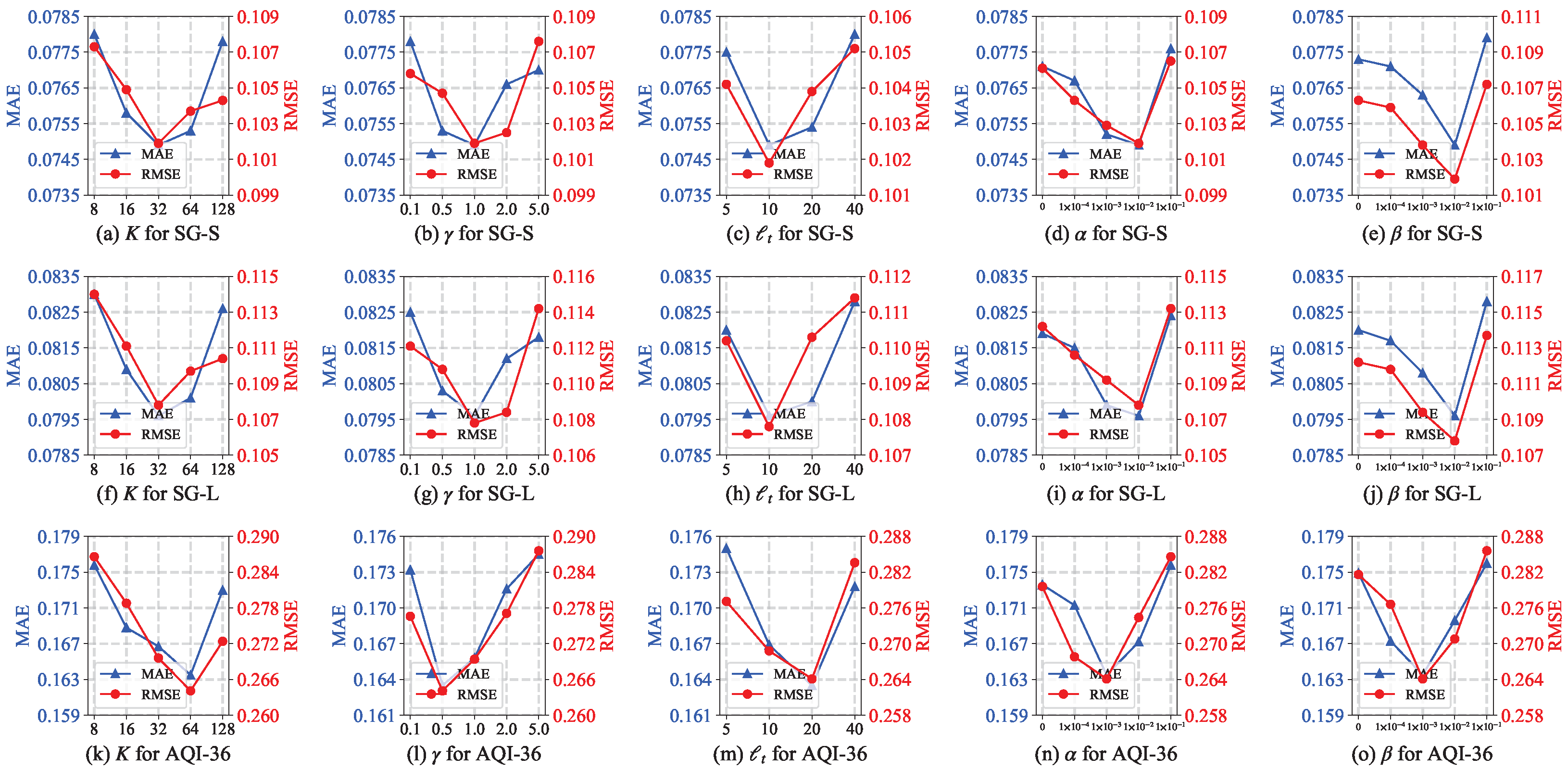
We analyzed the sensitivity of LG-MACFM to several important hyperparameters, including the number of selected observed positions K, the spatial diffusion coefficient $\gamma$, the temporal length scale ${\ell }_t$, and the regularization weights $\alpha$ and $\beta$. Unless otherwise specified, the experiments were conducted at a 50% missing rate.

As shown in Figure 2, LG-MACFM achieves stable performance within a reasonable range of hyperparameter settings. For the number of selected observed positions K, the performance first improves and then slightly degrades as K increases. This is because a small K may provide insufficient spatial and temporal context for the local joint GP-informed prior, while an overly large K may introduce weakly related observations and reduce locality. The best performance is obtained with $K=32$ on SG-S and SG-L and with $K=64$ on AQI-36.

For the spatial diffusion coefficient $\gamma$ and temporal length scale ${\ell }_t$, moderate values lead to better results. When $\gamma$ or ${\ell }_t$ is too small, the model can only capture limited spatial or temporal dependencies. In contrast, overly large values may introduce excessive smoothing of local spatio-temporal structures. The selected values are $\gamma =1.0$ and ${\ell }_t=10$ for SG-S and SG-L, whereas AQI-36 favors $\gamma =0.5$ and ${\ell }_t=20$.

For the regularization weights $\alpha$ and $\beta$, the best results are obtained at ${10}^{-2}$ on SG-S and SG-L and at ${10}^{-3}$ on AQI-36. Smaller weights provide limited uncertainty-aware or relation-matching supervision, while larger weights may over-constrain the endpoint or amplify fitting noise. Overall, these results indicate that LG-MACFM can maintain robust performance with properly selected settings.

5.7. Computational Efficiency Analysis

We evaluated computational efficiency on SG-L at a 50% missing rate using the experimental environment described in Section 5.2. As shown in

Table 8. Efficiency comparison on SG-L under a 50% missing rate. GPU memory denotes the maximum allocated device memory during training.

Model	Parameters	Training Time	Testing Time	GPU Memory
CSDI	1.76 M	52.8 s/epoch	34.6 s	7.8 GB
PriSTI	2.34 M	61.5 s/epoch	29.8 s	8.6 GB
Impute-MACFM	1.85 M	31.7 s/epoch	8.4 s	4.1 GB
TSFlow	2.12 M	36.9 s/epoch	10.2 s	4.6 GB
GiFlow	2.06 M	33.6 s/epoch	6.9 s	4.3 GB
LG-MACFM	2.18 M	38.4 s/epoch	8.9 s	5.2 GB

, LG-MACFM contains 2.18 M parameters and requires 38.4 s per training epoch, 8.9 s for testing, and 5.2 GB of peak GPU memory. It is substantially faster and more memory-efficient than the diffusion-based CSDI and PriSTI. Compared with the flow-based methods, LG-MACFM uses more memory because it maintains blockwise covariance matrices, while its testing time is lower than TSFlow but higher than Impute-MACFM and GiFlow. Together with the accuracy improvements in Table 5, these results indicate a practical balance between imputation performance and computational cost.

Let ${\mathcal{C}}_v$ denote the cost of one velocity-network evaluation, which scales approximately linearly with the window size $NL$ for a sparse spatial graph and fixed network settings. After selecting the top-K conditioning positions, the GP cost for Q missing blocks with sizes $m_q$ is ${\mathcal{C}}_{\mathrm{GP}}=\mathcal{O}\left({\sum }_{q=1}^Q{(K+m_q)}^3\right)$. The per-window training and single-sample inference costs are approximately $\mathcal{O}({\mathcal{C}}_v+{\mathcal{C}}_{\mathrm{GP}})$ and $\mathcal{O}(S{\mathcal{C}}_v+{\mathcal{C}}_{\mathrm{GP}})$, respectively, where S is the number of ODE steps. Since K is fixed and $m_q\le m_{max}$, the GP overhead grows approximately linearly with Q, avoiding the $\mathcal{O}\left({\left(NL\right)}^3\right)$ cost of a full GP over the complete window.

6. Conclusions

This paper proposes LG-MACFM for renewable energy generation data imputation. The proposed method constructs a local joint GP-informed source prior for each missing block from relevant observed spatio-temporal signals and uses a mask-aware conditional flow matching process to generate missing values while strictly preserving observed entries. Covariance-aware endpoint supervision weights endpoint errors according to source-prior uncertainty, while relation matching aligns predicted spatio-temporal differences with their target values. Experimental results show that LG-MACFM achieves better deterministic and probabilistic imputation performance than representative baselines across different missing rates. The ablation and sensitivity analyses further verify the effectiveness and robustness of the proposed components.

Future work will extend the current framework toward data-adaptive block partitioning and conditioning selection, sparse or learnable GP kernels, and dynamic graph construction, thereby accommodating more diverse correlation structures and large-scale systems. More efficient flow solvers and validation on larger multi-source renewable energy systems with naturally occurring missing patterns will also be explored.

References

1. Hong, T.; Pinson, P.; Wang, Y.; Weron, R.; Yang, D.; Zareipour, H. Energy forecasting: A review and outlook. IEEE Open Access J. Power Energy 2020, 7, 376–388. [Google Scholar] [CrossRef] [Scilit]
2. Antonanzas, J.; Osorio, N.; Escobar, R.; Urraca, R.; Martinez-de Pison, F.J.; Antonanzas-Torres, F. Review of photovoltaic power forecasting. Sol. Energy 2016, 136, 78–111. [Google Scholar] [CrossRef] [Scilit]
3. Golestaneh, F.; Gooi, H.B.; Pinson, P. Generation and evaluation of space–time trajectories of photovoltaic power. Appl. Energy 2016, 176, 80–91. [Google Scholar] [CrossRef] [Scilit]
4. Sweeney, C.; Bessa, R.J.; Browell, J.; Pinson, P. The future of forecasting for renewable energy. Wiley Interdiscip. Rev. Energy Environ. 2020, 9, e365. [Google Scholar] [CrossRef] [Scilit]
5. Du, J.; Hu, M.; Zhang, W. Missing data problem in the monitoring system: A review. IEEE Sens. J. 2020, 20, 13984–13998. [Google Scholar] [CrossRef] [Scilit]
6. Kuppannagari, S.R.; Fu, Y.; Chueng, C.M.; Prasanna, V.K. Spatio-temporal missing data imputation for smart power grids. In Proceedings of the Twelfth ACM International Conference on Future Energy Systems, Torino, Italy, 28 June–2 July 2021; pp. 458–465. [Google Scholar]
7. Mantuano, C.; Omoyele, O.; Hoffmann, M.; Weinand, J.M.; Panella, M.; Stolten, D. Data imputation methods for intermittent renewable energy sources: Implications for energy system modeling. Energy Convers. Manag. 2025, 339, 119857. [Google Scholar] [CrossRef] [Scilit]
8. Lee, D.S.; Son, S.Y. PV forecasting model development and impact assessment via imputation of missing PV power data. IEEE Access 2024, 12, 12843–12852. [Google Scholar] [CrossRef] [Scilit]
9. Kim, T.; Ko, W.; Kim, J. Analysis and impact evaluation of missing data imputation in day-ahead PV generation forecasting. Appl. Sci. 2019, 9, 204. [Google Scholar] [CrossRef] [Scilit]
10. Van Buuren, S.; Groothuis-Oudshoorn, K. mice: Multivariate imputation by chained equations in R. J. Stat. Softw. 2011, 45, 1–67. [Google Scholar] [CrossRef] [Scilit]
11. Mazumder, R.; Hastie, T.; Tibshirani, R. Spectral regularization algorithms for learning large incomplete matrices. J. Mach. Learn. Res. 2010, 11, 2287–2322. [Google Scholar]
12. Liao, W.; Bak-Jensen, B.; Pillai, J.R.; Yang, D.; Wang, Y. Data-driven missing data imputation for wind farms using context encoder. J. Mod. Power Syst. Clean Energy 2022, 10, 964–976. [Google Scholar] [CrossRef] [Scilit]
13. Liu, W.; Ren, C.; Xu, Y. Missing-data tolerant hybrid learning method for solar power forecasting. IEEE Trans. Sustain. Energy 2022, 13, 1843–1852. [Google Scholar] [CrossRef] [Scilit]
14. Bülte, C.; Kleinebrahm, M.; Yilmaz, H.Ü.; Gómez-Romero, J. Multivariate time series imputation for energy data using neural networks. Energy AI 2023, 13, 100239. [Google Scholar] [CrossRef] [Scilit]
15. Cini, A.; Marisca, I.; Alippi, C. Filling the g_ap_s: Multivariate time series imputation by graph neural networks. In Proceedings of the Tenth International Conference on Learning Representations, Virtual, 25–29 April 2022. [Google Scholar]
16. Marisca, I.; Cini, A.; Alippi, C. Learning to reconstruct missing data from spatiotemporal graphs with sparse observations. Adv. Neural Inf. Process. Syst. 2022, 35, 32069–32082. [Google Scholar] [CrossRef] [Scilit]
17. Wang, Y.; Peng, H.; Wang, S.; Du, H.; Liu, C.; Wu, J.; Wu, G. Stamimputer: Spatio-temporal attention moe for traffic data imputation. arXiv 2025, arXiv:2506.08054. [Google Scholar]
18. Fortuin, V.; Baranchuk, D.; Rätsch, G.; Mandt, S. Gp-vae: Deep probabilistic time series imputation. In Proceedings of the International Conference on Artificial Intelligence and Statistics; PMLR: Cambridge, CA, USA, 2020; pp. 1651–1661. [Google Scholar]
19. Tashiro, Y.; Song, J.; Song, Y.; Ermon, S. Csdi: Conditional score-based diffusion models for probabilistic time series imputation. Adv. Neural Inf. Process. Syst. 2021, 34, 24804–24816. [Google Scholar]
20. Liu, M.; Huang, H.; Feng, H.; Sun, L.; Du, B.; Fu, Y. Pristi: A conditional diffusion framework for spatiotemporal imputation. In Proceedings of the 2023 IEEE 39th International Conference on Data Engineering (ICDE); IEEE: New York, NY, USA, 2023; pp. 1927–1939. [Google Scholar] [CrossRef] [Scilit]
21. He, W.; Huang, J.; Gu, J.; Zhang, J.; Bai, Y. Filling the missings: Spatiotemporal data imputation by conditional diffusion. In Proceedings of the Thirty-Fourth International Joint Conference on Artificial Intelligence, Montreal, QC, Canada, 16–22 August 2025; pp. 2874–2882. [Google Scholar] [CrossRef] [Scilit]
22. Lipman, Y.; Chen, R.T.; Ben-Hamu, H.; Nickel, M.; Le, M. Flow matching for generative modeling. In Proceedings of the Eleventh International Conference on Learning Representations, Kigali, Rwanda, 1–5 May 2023. [Google Scholar]
23. Tong, A.; Malkin, N.; Huguet, G.; Zhang, Y.; Rector-Brooks, J.; Fatras, K.; Wolf, G.; Bengio, Y. Conditional flow matching: Simulation-free dynamic optimal transport. arXiv 2023, arXiv:2302.00482. [Google Scholar]
24. Liu, D.; Wang, H.; Fang, H. Impute-MACFM: Imputation based on Mask-Aware Flow Matching. arXiv 2025, arXiv:2509.23126. [Google Scholar]
25. Kollovieh, M.; Lienen, M.; Lüdke, D.; Schwinn, L.; Günnemann, S. Flow matching with gaussian process priors for probabilistic time series forecasting. In Proceedings of the International Conference on Learning Representations, Singapore, 24–28 April 2025; Volume 2025, pp. 95435–95457. [Google Scholar]
26. Zhang, Z.; Einizade, A.; Giraldo, J.H.; Fink, O. Spatiotemporal Imputation with Graph-Informed Flow Matching. In Proceedings of the International Conference on Machine Learning, Seoul, Republic of Korea, 6–11 July 2026. [Google Scholar]
27. Stekhoven, D.J.; Bühlmann, P. MissForest—non-parametric missing value imputation for mixed-type data. Bioinformatics 2012, 28, 112–118. [Google Scholar] [CrossRef] [Scilit]
28. Yi, X.; Zheng, Y.; Zhang, J.; Li, T. ST-MVL: Filling Missing Values in Geo-Sensory Time Series Data. In Proceedings of the IJCAI, New York, NY, USA, 9–15 July 2016; Volume 2016, pp. 2704–2710. [Google Scholar]
29. Che, Z.; Purushotham, S.; Cho, K.; Sontag, D.; Liu, Y. Recurrent neural networks for multivariate time series with missing values. Sci. Rep. 2018, 8, 6085. [Google Scholar] [CrossRef] [Scilit]
30. Cao, W.; Wang, D.; Li, J.; Zhou, H.; Li, L.; Li, Y. Brits: Bidirectional recurrent imputation for time series. Adv. Neural Inf. Process. Syst. 2018, 31, 6776–6786. [Google Scholar]
31. Yoon, J.; Zame, W.R.; Van Der Schaar, M. Estimating missing data in temporal data streams using multi-directional recurrent neural networks. IEEE Trans. Biomed. Eng. 2018, 66, 1477–1490. [Google Scholar] [CrossRef] [Scilit]
32. Bansal, P.; Deshpande, P.; Sarawagi, S. Missing value imputation on multidimensional time series. arXiv 2021, arXiv:2103.01600. [Google Scholar]
33. Du, W.; Côté, D.; Liu, Y. Saits: Self-attention-based imputation for time series. Expert Syst. Appl. 2023, 219, 119619. [Google Scholar] [CrossRef] [Scilit]
34. Nie, T.; Qin, G.; Ma, W.; Mei, Y.; Sun, J. ImputeFormer: Low rankness-induced transformers for generalizable spatiotemporal imputation. In Proceedings of the 30th ACM SIGKDD Conference on Knowledge Discovery and Data Mining, Barcelona, Spain, 25–29 August 2024; pp. 2260–2271. [Google Scholar]
35. Liu, S.; Li, X.; Cong, G.; Chen, Y.; Jiang, Y. Multivariate time-series imputation with disentangled temporal representations. In Proceedings of the Eleventh International Conference on Learning Representations, Kigali, Rwanda, 1–5 May 2023. [Google Scholar]
36. Jing, B.; Zhou, D.; Ren, K.; Yang, C. Causality-aware spatiotemporal graph neural networks for spatiotemporal time series imputation. In Proceedings of the 33rd ACM International Conference on Information and Knowledge Management, Boise, ID, USA, 21–25 October 2024; pp. 1027–1037. [Google Scholar]
37. Yoon, J.; Jordon, J.; Schaar, M. Gain: Missing data imputation using generative adversarial nets. In Proceedings of the International Conference on Machine Learning; PMLR: Cambridge, CA, USA, 2018; pp. 5689–5698. [Google Scholar]
38. Luo, Y.; Zhang, Y.; Cai, X.; Yuan, X. E2gan: End-to-end generative adversarial network for multivariate time series imputation. In Proceedings of the 28th International Joint Conference on Artificial Intelligence; AAAI Press: Palo Alto, CA, USA, 2019; pp. 3094–3100. [Google Scholar]
39. Miao, X.; Wu, Y.; Wang, J.; Gao, Y.; Mao, X.; Yin, J. Generative semi-supervised learning for multivariate time series imputation. In Proceedings of the AAAI Conference on Artificial Intelligence, Virtual, 2–9 February 2021; Volume 35, pp. 8983–8991. [Google Scholar]
40. Fang, S.; Wen, Q.; Luo, Y.; Zhe, S.; Sun, L. Bayotide: Bayesian online multivariate time series imputation with functional decomposition. arXiv 2023, arXiv:2308.14906. [Google Scholar]
41. Choi, M.; Lee, C. Conditional information bottleneck approach for time series imputation. In Proceedings of the International Conference on Learning Representations, Vienna, Austria, 7–11 May 2024; Volume 2024, pp. 51096–51117. [Google Scholar]
42. Alcaraz, J.M.L.; Strodthoff, N. Diffusion-based time series imputation and forecasting with structured state space models. arXiv 2022, arXiv:2208.09399. [Google Scholar]
43. Wang, X.; Zhang, H.; Wang, P.; Zhang, Y.; Wang, B.; Zhou, Z.; Wang, Y. An observed value consistent diffusion model for imputing missing values in multivariate time series. In Proceedings of the 29th ACM SIGKDD Conference on Knowledge Discovery and Data Mining, Long Beach, CA, USA, 6–10 August 2023; pp. 2409–2418. [Google Scholar] [CrossRef] [Scilit]
44. Zhou, J.; Li, J.; Zheng, G.; Wang, X.; Zhou, C. Mtsci: A conditional diffusion model for multivariate time series consistent imputation. In Proceedings of the 33rd ACM International Conference on Information and Knowledge Management, Boise, ID, USA, 21–25 October 2024; pp. 3474–3483. [Google Scholar]
45. Chen, Z.; Li, H.; Wang, F.; Zhang, O.; Xu, H.; Jiang, X.; Song, Z.; Wang, H. Rethinking the diffusion models for missing data imputation: A gradient flow perspective. Adv. Neural Inf. Process. Syst. 2024, 37, 112050–112103. [Google Scholar] [CrossRef] [Scilit]
46. Weber, M.; Turowski, M.; Çakmak, H.K.; Mikut, R.; Kühnapfel, U.; Hagenmeyer, V. Data-driven copy-paste imputation for energy time series. IEEE Trans. Smart Grid 2021, 12, 5409–5419. [Google Scholar] [CrossRef] [Scilit]
47. Li, Q.; Xu, Y.; Chew, B.S.H.; Ding, H.; Zhao, G. An integrated missing-data tolerant model for probabilistic PV power generation forecasting. IEEE Trans. Power Syst. 2022, 37, 4447–4459. [Google Scholar] [CrossRef] [Scilit]
48. Sun, C.; Chen, Y.; Cheng, C. Imputation of missing data from offshore wind farms using spatio-temporal correlation and feature correlation. Energy 2021, 229, 120777. [Google Scholar] [CrossRef] [Scilit]
49. de Paz-Centeno, I.; Garcia-Ordas, M.T.; García-Olalla, Ó.; Alaiz-Moreton, H. Imputation of missing measurements in PV production data within constrained environments. Expert Syst. Appl. 2023, 217, 119510. [Google Scholar] [CrossRef] [Scilit]
50. Williams, C.K.; Rasmussen, C.E. Gaussian Processes for Machine Learning; MIT Press: Cambridge, MA, USA, 2006; Volume 2. [Google Scholar]
51. Troyanskaya, O.; Cantor, M.; Sherlock, G.; Brown, P.; Hastie, T.; Tibshirani, R.; Botstein, D.; Altman, R.B. Missing value estimation methods for DNA microarrays. Bioinformatics 2001, 17, 520–525. [Google Scholar] [CrossRef] [Scilit]
Figure 1. Overview of LG-MACFM for renewable energy imputation.
Information 17 00842 g001
Figure 2. Hyperparameter sensitivity analysis of LG-MACFM on SG-S, SG-L, and AQI-36 at a 50% missing rate.
Information 17 00842 g002