Article

Preference Learning and Hybrid Combinatorial Optimization for Intelligent Group-Buying Platforms: A Prototype-Calibrated Study of SmartBuy Connect


1
Information Systems Department, Satbayev University, Almaty 050013, Kazakhstan
2
Department of Computer Engineering, Gachon University, Sujeong-Gu, Seongnam-Si 461-701, Republic of Korea
3
Software Engineering Department, Satbayev University, Almaty 050013, Kazakhstan
*
Author to whom correspondence should be addressed.
Information 2026, 17(8), 768; https://doi.org/10.3390/info17080768
Submission received: 29 June 2026 / Revised: 28 July 2026 / Accepted: 4 August 2026 / Published: 11 August 2026
(This article belongs to the Special Issue Decision-Making Process in E-Commerce and Social Networks)

Abstract

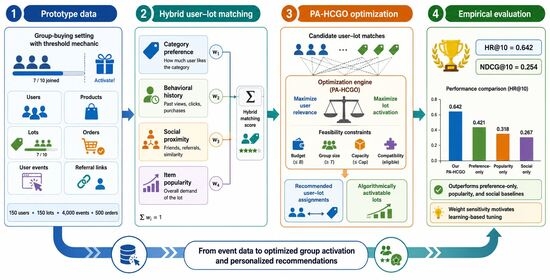
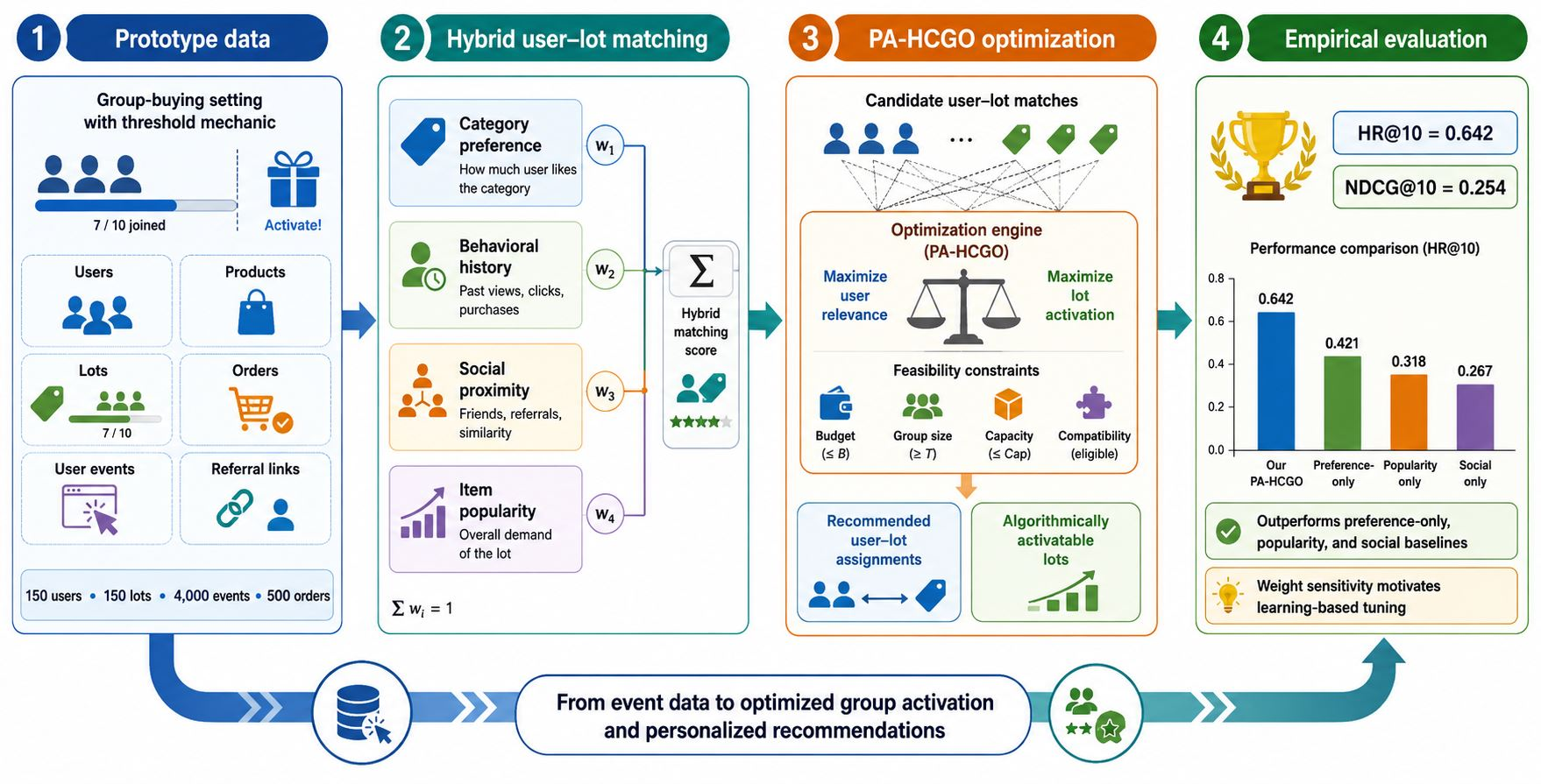
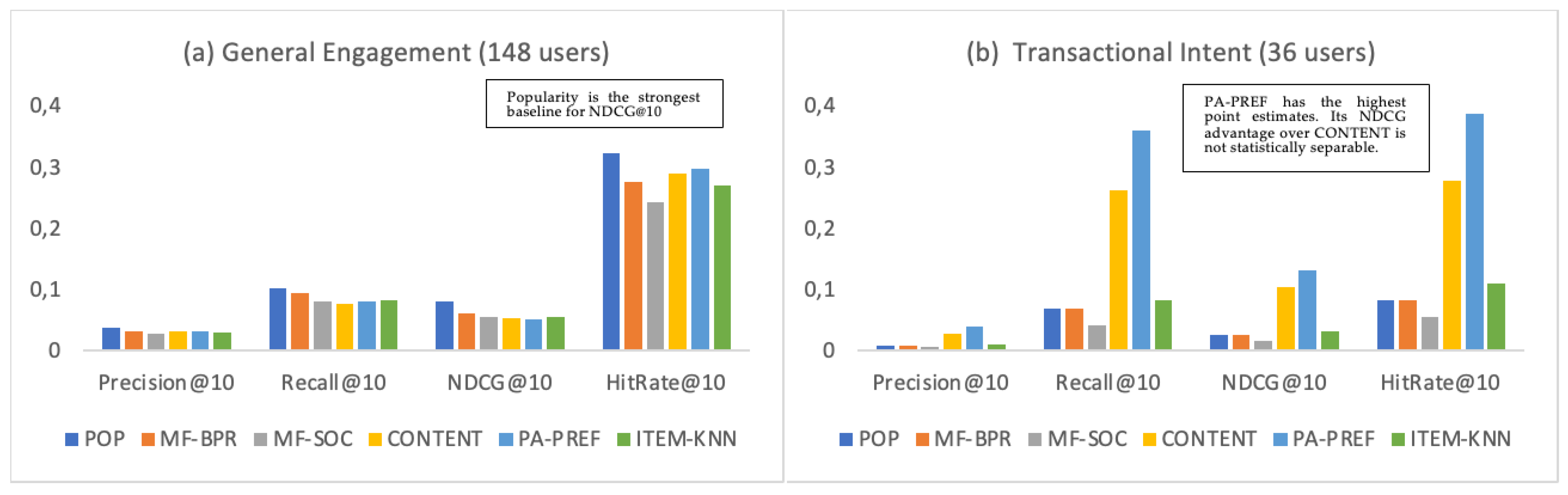
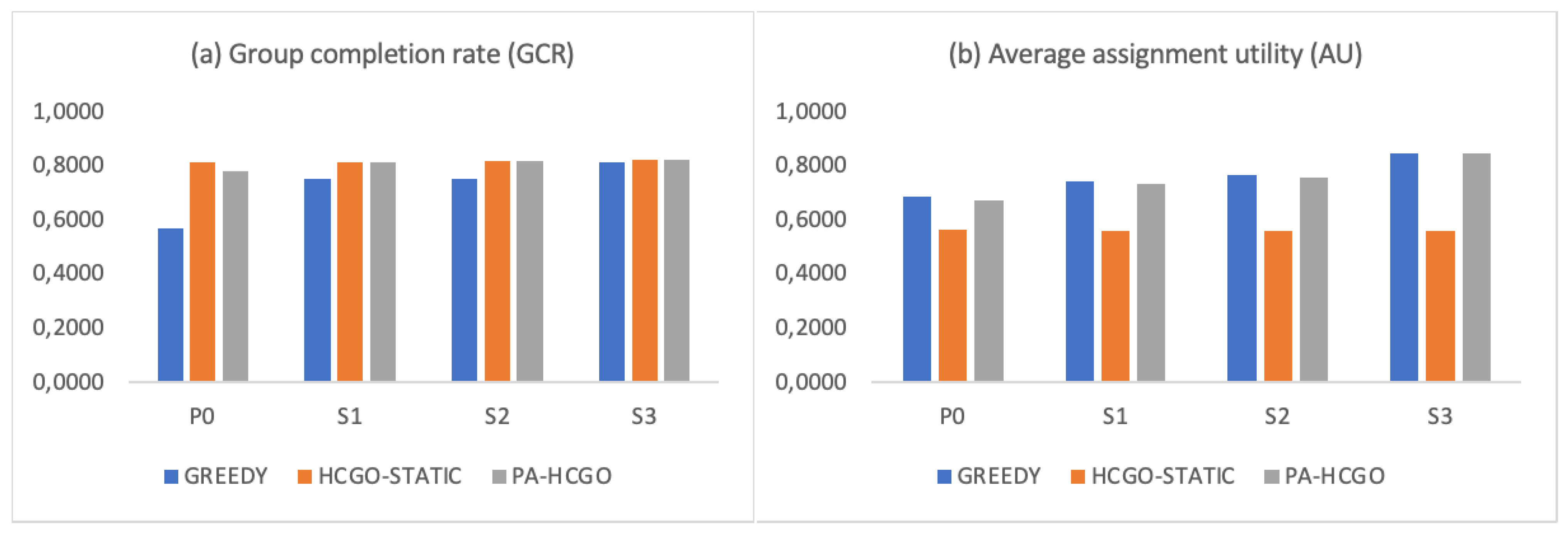
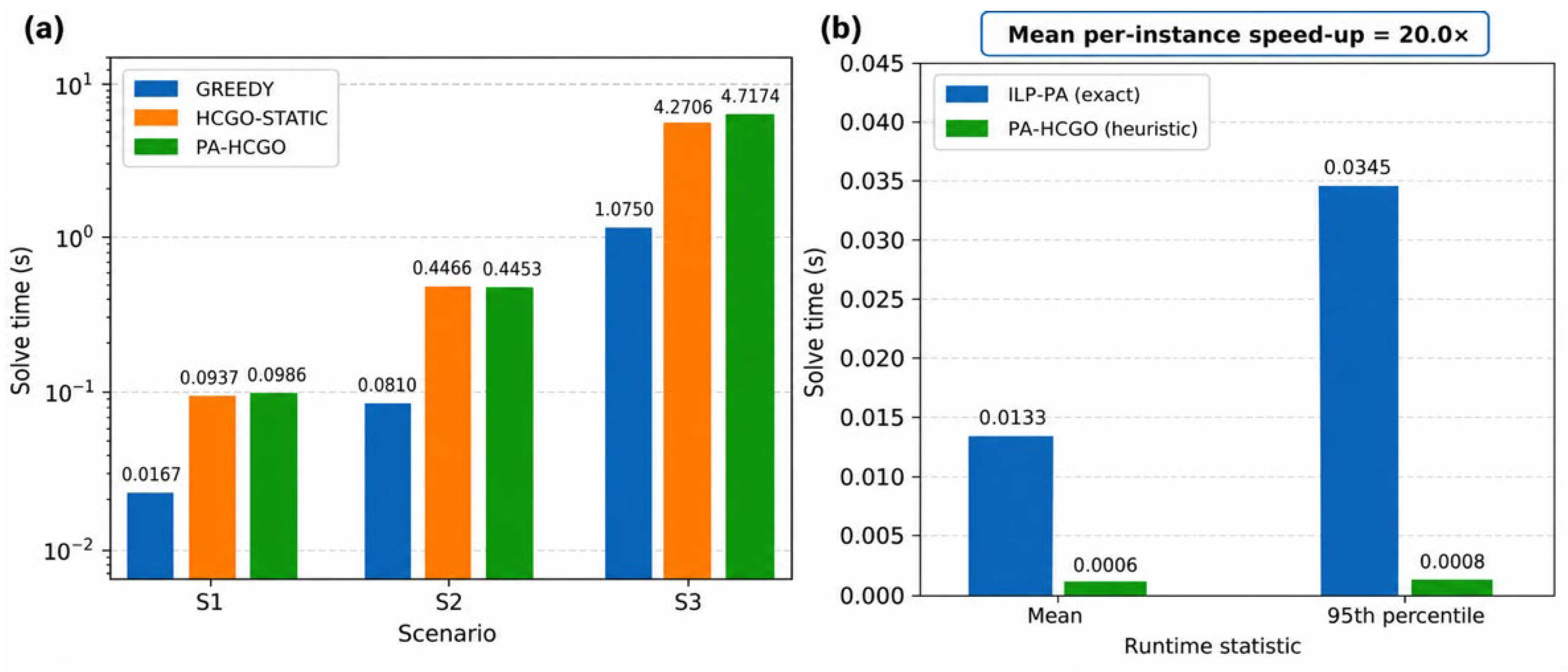
Group-buying platforms require the joint treatment of individual user relevance and hard operational constraints, including minimum group size, lot capacity, spending limits, product availability, and simultaneous participation limits. This paper presents Preference-Aware Hybrid Combinatorial Group Optimization (PA-HCGO), a prototype-calibrated decision framework that integrates implicit feedback preference learning with constrained user–lot assignment. The contribution is not a new recommender architecture or a new integer programming solver, but a system-level integration of learned user–lot utility and hard group-buying feasibility constraints inside the SmartBuy Connect prototype. The empirical part uses an anonymized prototype dataset containing 200 products, 150 users, 150 lots, 4000 user events, and 500 orders. The evaluation is explicitly divided into three tracks: observed temporal recommendation testing, a calibrated counterfactual pre-activation scenario, and synthetic scalability tests generated from prototype-calibrated distributions. In the observed transactional test subset, which contains 40 held-out transactional items from 36 users, the PA-PREF preference layer achieved Recall@10 = 0.3611 and NDCG@10 = 0.1319 using user–category profiles available at the end of the training interval. Although PA-PREF obtained the highest point estimate, its advantage over the content-only baseline was not statistically separable at the 95% level on this small transactional subset. The result is therefore treated as preliminary. For general engagement, the popularity baseline remained stronger, indicating that the proposed preference model is more useful for transactional intent prediction than for all activity types. In the calibrated counterfactual pre-activation scenario, PA-HCGO activated 117 of 150 lots, compared with 85 lots under independent greedy assignment. This scenario is a constructed pre-activation setting rather than an observed historical platform state. In synthetic scalability tests, the method remained computationally feasible up to 5000 users and 1000 lots, with a mean solve time of 4.7174 s in the prototype implementation. The results suggest that learned user–lot utility can improve constrained group formation, but the evidence should be interpreted as prototype-calibrated rather than as proof of industrial-scale business effectiveness.

Graphical Abstract

1. Introduction

E-commerce is gradually moving away from the single-transaction model toward platform mechanisms. In these mechanisms, value comes from aggregated demand, social interaction, and the algorithmic coordination of users. Group buying is a typical example. A commercial offer is activated once a target number of participants is reached. The seller then gains a predictable sales volume, and the buyers gain a price advantage. The economics of threshold mechanisms and the way the outcome depends on the structure of demand were shown in early studies of web group buying [1,2].
Forming groups is not only a pricing task. It is also a coalition task. Users differ in their interests, their budget, and their willingness to join several purchases. Products have availability limits, and lots have a minimum size and a maximum capacity. Work on buyer coalition formation and on multi-item group buying has formalized separate parts of this allocation problem [3,4]. Related research on group-buying-based combinatorial reverse auctions has further demonstrated the benefits of coordinated group-buying mechanisms over independent procurement schemes under combinatorial constraints [5]. Studies of fairness and incentive mechanisms further showed that participation depends on the auction rules and on how users perceive the terms of the deal [6]. In social commerce, value also comes from network ties, referral spreading, and mutual influence between users [7,8].
Alongside the growth of group buying, artificial intelligence has become a systemic component of e-commerce. Its use covers personalization, forecasting, intelligent agents, risk management, and the optimization of platform decisions [9]. Most practical systems, however, keep the recommendation loop and the operational loop separate. The first one ranks products, and the second one controls orders and constraints. As a result, a personally relevant offer may be useless for completing a specific lot, while an optimally filled group may include users with little interest in the product.
Classic matrix factorization and ranking from implicit feedback can recover hidden preferences from views, searches, lot joins, and orders [10,11]. Neural Collaborative Filtering extends this idea by capturing non-linear user–item interactions [12], and surveys of deep recommender systems organize the strengths and the limits of such models [13]. Their typical output is still a ranking of items rather than a coordinated decision for the whole set of users.
Graph models strengthen the recommendation layer through structural dependencies. Basic architectures for graph convolution, inductive aggregation, and graph attention formed the foundation of modern graph representation learning [14,15,16]. In recommender systems, these ideas appear in NGCF, LightGCN, and social graph models [17,18,19]. Surveys show that graph neural networks are especially useful for complex user–item and user–user relations, yet their integration with downstream constrained decisions is still an open problem [20,21].
The related area of group recommendation studies how to choose an item for a group that already exists [22,23,24]. The group-buying task has the opposite logic. Here, the system must form or top up several groups out of a pool of users. For this reason, aggregating the preferences of an existing group does not replace the optimization of user–lot assignments. The cold-start problem adds further difficulty. New users have little history, so the system must rely on content or context features [25,26].
Strict respect for budget, capacity, and thresholds is naturally expressed through integer programming [27]. For large instances, metaheuristics and hybrid procedures are used [28]. The modern line of learning-augmented combinatorial optimization suggests using predictive models to set the coefficients of the objective, to reduce the search space, and to select the solver [29,30,31,32]. This logic provides a methodological basis for joining a recommendation score with group optimization.
Dynamic pricing is also linked to the probability that a lot will be completed, and it can become a later layer of platform intelligence [33,34]. Still, the joint optimization of price and group composition requires a more basic question to be solved first. That question is how to turn heterogeneous behavioral and social signals into a utility for a user–lot pair, and then how to form feasible assignments across the whole platform.
This study proposes Preference-Aware Hybrid Combinatorial Group Optimization (PA-HCGO). In this framework, a learned user–product compatibility is combined with the context of a specific lot and then used inside a binary multi-group assignment problem. The model accounts for the minimum group size, the capacity, the remaining budget, the maximum number of participations, and the feasibility of a user–lot pair. Small instances are solved exactly. Large instances use an activation-oriented heuristic followed by local improvement.
The application environment is SmartBuy Connect, a prototype group-buying platform with a buyer loop and a seller loop. Unlike fully synthetic studies, the experimental strategy uses an exported prototype dataset for training and calibration, and scaled scenarios for testing computational stability. This design separates empirically observed relations from scenario assumptions, and it makes the limits of external validity explicit.
The research problem is to design a method that does several things at once. It must score the individual relevance of lots, account for social and content signals, support users with little history, and form feasible groups under hard platform constraints. The aim of this study is to develop PA-HCGO as the intelligent core of SmartBuy Connect and to test it experimentally.
Four connected tasks serve this aim. The first is to build a temporally correct preference model from implicit feedback. The second is to formalize multi-group user–lot assignment. The third is to design a hybrid exact-and-heuristic solution procedure. The fourth is to check ranking quality, group completion, and computational scalability on prototype and calibrated data.
Terminology is used as follows: PA-PREF denotes the preference learning layer that produces user–product and user–lot utility scores from behavioral, content, and limited referral information. PA-HCGO denotes the full decision framework that uses these learned utilities inside a constrained group-buying assignment model. The term learned user–lot utility refers to the score used as an objective coefficient in the optimization problem. The term hybrid model is avoided unless the specific component is identified, because preference learning and constrained optimization play different roles in the framework.
The contribution of this paper is deliberately framed as a prototype-calibrated system integration contribution. This paper does not claim to introduce a fundamentally new recommender architecture or a new integer programming solver. Instead, it contributes a reproducible formulation and evaluation of how learned user–lot utility can relate to hard feasibility constraints in an intelligent group-buying platform.
The contribution is threefold. First, this paper formulates group-buying recommendation as a constrained user–lot assignment problem in which learned utility scores become objective coefficients, while minimum group size, capacity, stock, spending, and simultaneous participation constraints remain explicit. Second, it presents PA-HCGO as an integration framework that connects implicit feedback preference learning, content/cold-start scoring, feasibility filtering, and binary group assignment, while allowing limited referral information to be incorporated as an exploratory optional signal. Third, it provides a transparent prototype-calibrated evaluation protocol that separates observed temporal recommendation testing, calibrated counterfactual group activation analysis, and synthetic scalability testing.
To avoid overclaiming, PA-HCGO is positioned as an integration framework rather than as a replacement for state-of-the-art recommender architectures or commercial optimization solvers. The goal is to show how learned user–lot utility can be connected with feasibility-preserving group-buying assignment in a prototype platform. Therefore, the experimental comparison focuses on representative baselines that isolate the roles of popularity, matrix factorization, social information, static utility optimization, greedy feasible assignment, and exact preference-aware optimization on small instances. Stronger deep learning recommenders and advanced mathematical programming accelerations are treated as important extensions rather than as the central claim of this paper.
The scope of empirical evidence in this study is intentionally limited and explicitly separated into three evaluation tracks. First, observed prototype data are used for temporal recommendation testing and for estimating user–product preference signals. This track evaluates ranking quality on held-out interactions and, separately, on a smaller transactional subset. Second, the group activation experiment P0 is treated as a calibrated counterfactual pre-activation scenario. It does not reconstruct an actual historical sequence of lot joins because the exported lot table stores the final lot state rather than the full sequence of intermediate states. Third, the S1–S3 scenarios are synthetic scalability tests generated from empirical distributions observed in the prototype dataset. They are used to evaluate computational behavior and robustness under larger problem sizes, but they should not be interpreted as evidence of real market behavior or industrial business effectiveness.
This framing is central to this paper. The proposed method is evaluated as a prototype-calibrated decision framework rather than as a deployed commercial recommender system. The results support the technical feasibility of integrating learned user–lot utility with hard group-buying constraints, while leaving large-scale online validation, user acceptance probability, seller-side strategic behavior, and dynamic pricing for future work.
The remainder of this paper is organized as follows. Section 2 reviews prior work on group buying, social commerce, recommender systems, graph-based recommendation, cold-start handling, and learning-augmented combinatorial optimization. Section 3 describes the SmartBuy Connect prototype architecture and its data-generating components. Section 4 formalizes the user–lot assignment problem, defines the PA-HCGO model, and presents the exact and heuristic solution procedures. Section 5 describes the dataset, preprocessing, temporal split, calibrated scenarios, baselines, parameter settings, and evaluation metrics. Section 6 reports the experimental results for recommendation quality, group formation, exact solution comparison, scalability, ablation, and sensitivity analysis. Section 7 discusses the theoretical and practical implications, threats to validity, limitations, and future research directions. Section 8 concludes this paper and outlines future research directions.

2. Literature Review

Group buying rests on the threshold activation of a deal and on savings from aggregated demand. Anand and Aron [1] compared price-discovery mechanisms in web group buying and showed that efficiency depends on the heterogeneity of demand and on the pricing rules. Jing and Xie [2] read group buying as a mechanism that sells through social interaction, in which informed users help to attract others.
The coalition literature treats buyers as agents that can join forces for a volume discount. Yamamoto and Sycara [3] proposed a stable scheme for buyer coalition formation, and Li et al. [4] formalized multi-item group buying with heterogeneous buyers. These works are close to our task, but they use fixed preferences and do not rely on learned behavioral scores.
The economic rationale of group buying is demand aggregation. When several buyers coordinate their demand, the platform can create conditions for lower unit prices, higher seller-side order volume, and more efficient allocation of limited offers. This mechanism has been studied not only in consumer-oriented online group-buying markets but also in procurement and combinatorial auction settings. Hsieh and Lin [5] showed that a group-buying-based combinatorial reverse auction can outperform multiple independent combinatorial reverse auctions in terms of both performance and computational efficiency. This finding is important for the present study because PA-HCGO also treats group buying as a constrained coordination problem rather than as a simple discount-promotion mechanism.
However, the setting of SmartBuy Connect differs from procurement-oriented group-buying auctions. The platform does not aggregate fixed procurement requirements submitted by organizations. Instead, it must recommend feasible lots to individual users whose preferences are learned from implicit behavior, content signals, and limited referral information. Therefore, the challenge is not only to aggregate demand, but also to decide which users should be invited to which lots so that individual relevance and group activation are jointly optimized.
Studies of online group-buying auctions show the role of incentives and perceived fairness [6]. Social commerce extends this logic through interaction inside digital networks [7,8]. Economic and behavioral models, however, usually do not provide an algorithm for distributing users across many parallel lots.
The bibliometric and content review by Bawack et al. [9] shows that AI in e-commerce spans recommendation, personalization, trust, automation, and optimization. For a group-buying platform the key shift is from an isolated recommendation service to a loop in which user events turn into a decision about the state of a lot. Most of the reviewed e-commerce work analyzes separate AI functions but does not link them to threshold activation of groups under hard constraints.
Matrix factorization places users and products in a shared latent space and remains a strong personalization baseline [10]. For event logs without explicit ratings, Bayesian Personalized Ranking is particularly useful because it learns the relative order of positive and unobserved items [11]. Neural Collaborative Filtering replaces the dot product of embeddings with a neural interaction function [12]. The survey by Zhang et al. [13] shows that deep recommender systems improve the modeling of complex dependencies, yet their output is usually a top-N list with no guarantee that a downstream decision is feasible.
Graph convolutional networks [14], GraphSAGE [15], and graph attention networks [16] established the basic mechanisms for aggregating neighbors. In recommendation, NGCF [17] models high-order propagation of the collaborative signal, and LightGCN [18] simplifies the graph architecture down to embedding propagation. GraphRec joins user–item and user–user relations [19]. Recent surveys confirm the strong performance of GNNs in recommendation, but they single out cold start, computational cost, and integration with decision systems as open issues [20,21].
Group recommendation selects an item for a group that already exists and uses rules to aggregate individual preferences [22,23]. Attentive group recommendation also accounts for the unequal contribution of members [24]. In SmartBuy Connect, the group is not given in advance. The algorithm must distribute users across lots to reach the thresholds. Group recommendation methods are therefore a useful theoretical basis, but they do not solve constrained group-buying assignment.
The cold-start problem arises when a new user or product has too little history. Schein et al. [25] organized the methods and metrics for cold-start recommendation. DropoutNet trains a model to be robust to missing user or item representations [26]. This component matters for a prototype platform because a large share of users has a short history, while a complex collaborative model can overfit.
Binary integer programming enforces budget, capacity, and threshold constraints in a formal way [27]. As the size grows, metaheuristic and hybrid methods are used [28]. Bengio et al. [29] described ways to apply machine learning to combinatorial optimization, including search-space reduction and the learning of heuristics. Kotary et al. [30] surveyed end-to-end constrained optimization learning, and Mazyavkina et al. [31] surveyed reinforcement learning for combinatorial tasks. Talbi [32] proposed a taxonomy for integrating machine learning and metaheuristics. PA-HCGO follows a more interpretable scheme. A learned model produces utility scores, and a separate optimizer then enforces feasibility.
Dynamic pricing can account for how full a group is, the remaining time, and a demand forecast. Recent work shows the use of machine learning for adaptive pricing in e-commerce [33], and the systematic review by Chenavaz and Dimitrov [34] stresses the need to account for transparency, fairness, and trust. In this study, the price is treated as a fixed parameter of the lot. Joint optimization of group composition and price is left for later work.
The review shows that existing studies form an important theoretical and methodological basis, but no single line of work covers the task in full. Economic models explain the nature of collective demand and threshold activation, yet they rarely formalize the distribution of users across many lots. Coalition approaches account for group formation, but they usually do not use learned preferences. Recommender and graph models improve personalization, yet they do not guarantee that budget, capacity, and thresholds are met. Combinatorial optimization handles constraints strictly, but it often assumes that the utility is already given.
To position the proposed approach more clearly, the key research directions are compared in Table 1. The comparison shows which parts of the intelligent group-buying task are already covered in the literature, and which remain weakly integrated. Special attention is given to learning user preferences, accounting for social ties, respecting hard constraints, supporting cold-start users, and practical platform implementation.
As Table 1 shows, existing studies mostly solve separate parts of the task. Economic models explain the mechanisms of collective demand, recommender and graph models score individual and socially driven preferences, and combinatorial optimization formalizes the constraints. The gap is not the absence of separate methods. It is the absence of their coordinated integration inside a single platform architecture. Prior optimization-oriented studies, including Hsieh and Lin, show the value of coordinated group-buying mechanisms, but they do not solve the consumer-facing problem of learning user-specific preferences and using them as coefficients in a constrained assignment model.
The gap identified in Table 1 is therefore not the absence of recommendation models or optimization methods as separate tools. The gap is the lack of a transparent platform-level formulation that connects learned preference scores with feasibility-preserving group-buying assignment. In this sense, the novelty of PA-HCGO lies in the integration of components under group-buying constraints, rather than in proposing a new standalone recommender model or a new exact optimization algorithm.
The proposed PA-HCGO is meant to close this gap. It uses learned user–lot utility scores, accounts for referral links, supports new users, and forms groups through a hybrid mechanism. Unlike fully synthetic formulations, this study relies on the prototype structure of SmartBuy Connect, on temporal testing of the recommendation layer, and on calibrated scaling scenarios.
Based on this research gap, the next section describes the architecture of SmartBuy Connect and the place of PA-HCGO in the overall loop of data collection, preference learning, and group formation.

3. Architecture and Software Implementation of SmartBuy Connect

3.1. Architectural Requirements

A practical implementation of intelligent group buying needs an architecture that joins user interfaces, transactional business logic, behavioral data collection, and computational decision support. Unlike traditional e-commerce, the process does not end with an individual order. The system must support time-dependent filling of a lot, to track when the threshold is reached, to account for capacity, and to synchronize the actions of buyers and sellers.
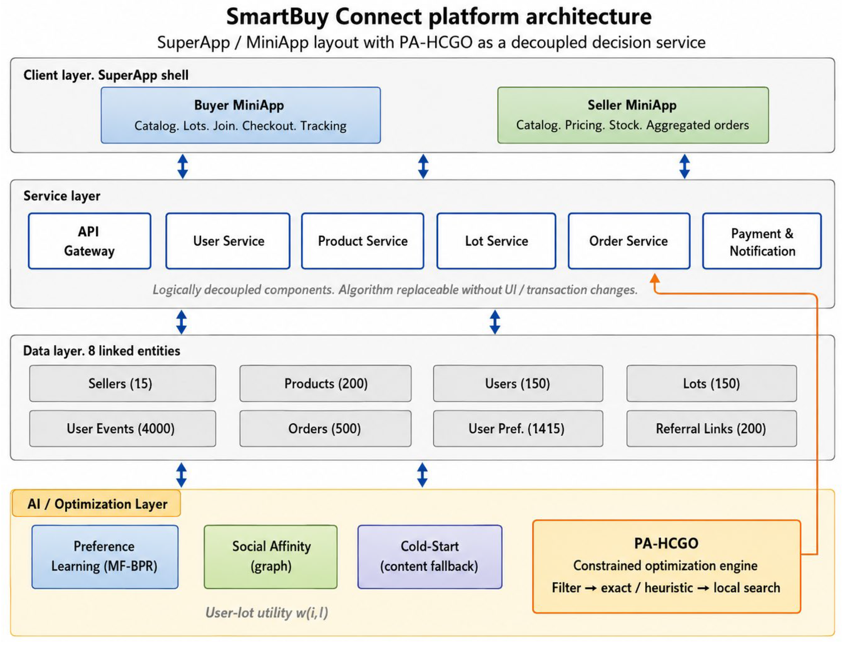
SmartBuy Connect is built as a SuperApp/MiniApp prototype. The SuperApp forms a shared digital environment for identity, the catalog, lots, orders, payment flows, and notifications. The MiniApp components implement the specialized buyer and seller loops. This separation lets the applied services and the intelligent core evolve independently.
The architecture was designed around four requirements: an end-to-end lifecycle of the group deal, structured logging of implicit feedback, a match between application entities and the parameters of the optimization model, and independent updates of the recommendation and optimization components.
The overall platform architecture is shown in Figure 1.
The architecture includes the client MiniApps, the service layer, the layer of operational and behavioral data, and the AI/optimization layer. Optimization results return to the applied services as a ranking of lots, feasible recommendations, and group activation decisions. The two-way data flow links user actions with the later update of the models.

3.2. Lifecycle of a Group Purchase

The buyer loop supports browsing the catalog, product cards, and active lots, creating a new group, joining an existing one, placing an order, and tracking its state. Viewing, searching, sharing an offer, creating and joining a lot, moving to checkout, and ordering are all logged as events of different strength.
A lot is linked to a product and holds a minimum number of participants, a maximum capacity, a time window, and a current state. Once the threshold is reached, it becomes an aggregated order. In the intelligent mode, the system ranks the available groups not only by individual relevance, but also by the system-level need to fill them.
The seller loop supports catalog, price, and stock management, the receipt of aggregated orders, and changes to fulfillment status. The prototype therefore covers the full digital cycle, from the appearance of demand to the confirmation and fulfillment of a group deal.

3.3. Service Layer and Separation of Responsibilities

External requests pass through an API Gateway. The User Service stores anonymized profiles and activity history. The Product Service manages products, categories, and sellers. The Lot Service handles the creation, filling, and completion of lots. The Order Service links the collective deal with individual orders. The Payment and Notification Service handles payment methods and informs participants.
PA-HCGO is treated as a separate decision service. It receives the prepared state of users and lots, forms the set of feasible pairs, and returns assignments to the Lot Service. This separation lowers the coupling of the system and lets the algorithm be changed without reworking the user interface or the transactional modules.
In this paper, the term service denotes a logically separate component. The prototype is not used as proof of a full industrial microservice deployment. The scalability of the architecture requires separate load and integration testing.

3.4. Data Layer

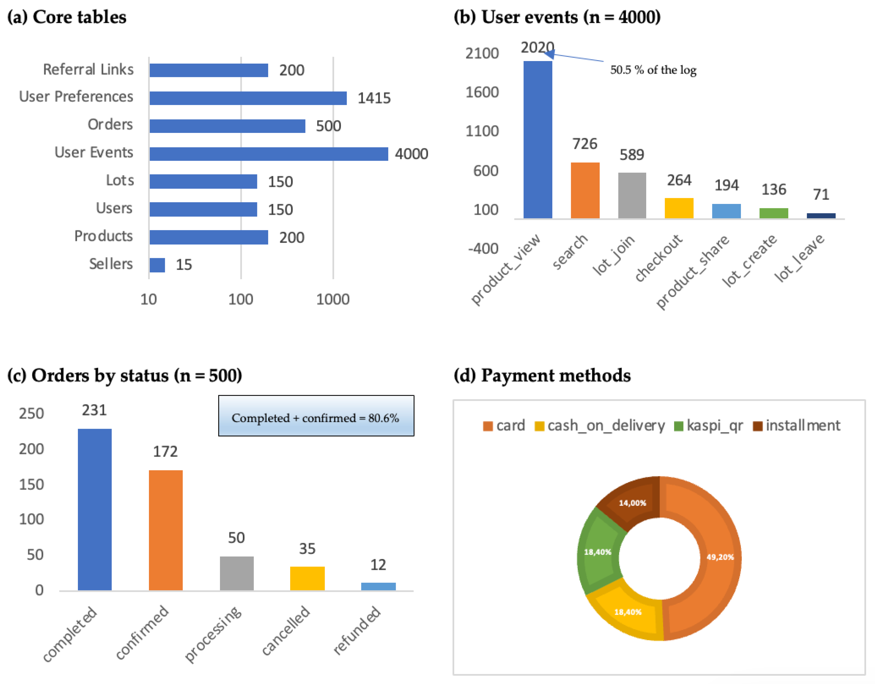
The data are organized around eight linked entities: sellers, products, users, lots, user events, orders, user preferences, and referral links. The identifiers allow the relations to be reconstructed without direct personal data. A product is linked to a seller, a lot to a product and its initiator, an event to a user and an interaction object, and an order to a user, a lot, a product, and a seller.
The composition of the prototype dataset, together with its detailed tabular structure, behavioral-event distribution, cleaning procedure, and temporal-split protocol, is presented in Section 5.
The most representative source is the set of 4000 user events. Their count exceeds the number of users and products because each profile generates a sequence of actions. The presence of orders and referral links allows transactional intent and the social component to be evaluated separately. The volume of data, however, remains typical of a controlled prototype rather than an industrial platform.

3.5. Intelligent Layer

The Preference Learning Module turns behavioral history into a score of user–product compatibility. The Social Affinity Module uses the referral graph, and the Cold-Start Module forms an initial score from the available categorical and contextual features. PA-HCGO adds the state of the lot to the product score and solves a constrained assignment problem.
The separation of learning and optimization is essential. A high predicted relevance is not an automatic assignment. A user may exceed the budget, a lot may be full, and a locally attractive allocation can reduce the number of completed groups. The optimization layer reconciles the individual scores at the level of the whole system.

3.6. Closed Decision Loop

The interaction of the components forms a closed decision loop.
A user action is logged and linked to a product or a lot. The prepared data update the preference scores. PA-HCGO computes a feasible allocation. The result is passed to the interface, and the user reaction becomes a new observation. The preference model can be updated in batches, while the optimization of active lots runs more often, as group states change.

3.7. Match Between the Architecture and the Research Model

Users and products define the main sets, lots define the thresholds and capacity, user events and orders provide the behavioral and transactional signals, user preferences provide the aggregated interests, and referral links provide the social graph. Each parameter of the mathematical model has a data source, and each binary decision has a corresponding platform action. This traceability gives a reproducible context for the formalization of PA-HCGO in the next section.

4. Materials and Methods

4.1. Study Design

This study consists of applied computational work. It joins data from the SmartBuy Connect software prototype, developed in-house at Satbayev University (Almaty, Kazakhstan), with preference learning and constrained combinatorial optimization. The methodological logic separates three connected but distinct levels: extracting behavioral signals from platform data, scoring the individual relevance of products and lots, and forming a feasible decision at the level of the whole system.
Unlike a fully synthetic scheme, the parameters of users, products, lots, orders, and referral links are taken from the SmartBuy Connect prototype set. The synthetic extension is used only when testing computational scalability and the stability of the algorithm as the number of users, products, and simultaneously active groups grows. This design keeps the experiment tied to the actual structure of the platform, and it still allows the study of cases that cannot yet be drawn from the limited prototype data.
The method has five sequential stages. First, the source tables are cleaned, linked, and encoded. Second, user events are turned into a weighted implicit feedback matrix. Third, a model of user–product compatibility is trained, joining the behavioral, social, and content signals. Fourth, the product scores are extended with the context of a specific lot. Fifth, the resulting scores are used as the coefficients of the objective in a binary optimization problem.
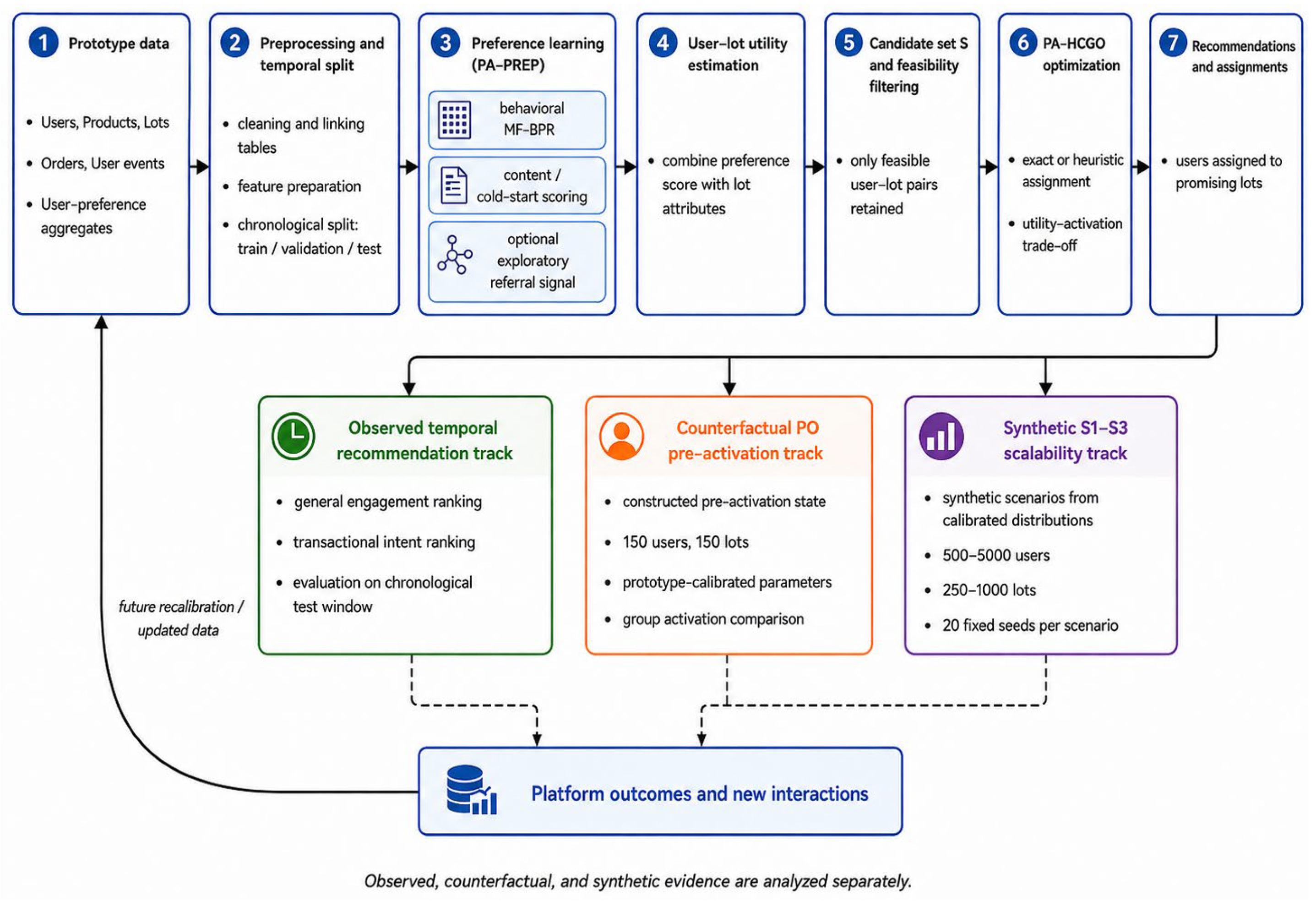
The complete PA-HCGO methodology and the three-track evaluation design are summarized in Figure 2.
As Figure 2 shows, the learned component and the optimization component play different roles. The preference model answers how well a given product or lot matches a user’s interests. The optimization module decides which assignments to carry out at the platform level, given the minimum group size, the capacity, the allowed number of participations, product availability, and spending limits. This separation rules out the case where a high predicted score is read directly as a final decision.

4.2. Problem Statement and Decision Variables

The operational problem solved by PA-HCGO is the following: At a given decision moment, the platform observes a set of users who may receive group-buying recommendations, a set of active lots that have not yet reached or have just approached their activation thresholds, and a set of products linked to these lots. For each feasible user–lot pair, the preference learning layer provides a normalized utility score. The task is to select which lots should be prioritized for activation, and which users should be recommended to these lots, while respecting hard constraints on minimum group size, lot capacity, product stock, user spending limits, and the maximum number of simultaneous group participations.
The model therefore does not solve a standard top-N recommendation problem. A high utility score alone is not sufficient for assignment because the assignment must also help satisfy group-buying constraints. Conversely, activating many lots without considering user relevance can produce low-quality recommendations. The mathematical problem is to maximize a normalized combination of user–lot utility and lot activation under feasibility constraints. The decision returned by the model is an assignment recommendation, not an automatic purchase.
Let the set of platform users be:
U = { u 1 , u 2 , , u n }
The set of products is:
P = { p 1 , p 2 , , p h }
and the set of active group lots is:
L = { l 1 , l 2 , , l m }
Each lot l L is linked to one product p ( l ) P . A separate set of lots is needed because the same product can appear in several groups with different time windows, prices, capacities, or current member counts.
When the algorithm starts, the number of users who have already joined a lot, n l 0 , is known for each lot. The basic batch formulation considers lots that have not yet reached the activation threshold:
0 m l 0 < q l c l ,    l L
where q l is the minimum group size and c l is the maximum lot capacity.
For every potential user–lot pair, we introduce a binary variable:
x i l { 0 , 1 } , i U ,   l L
The value x i l = 1 means that user i is included in the optimized set of participants of lot l . The value x i l = 0 means that no such assignment is carried out. In the platform interface, this decision is read as a priority recommendation that the user still must confirm.
For each lot, we also define a binary activation variable
y l { 0 , 1 } ,    l L
The variable y l equals 1 if, after adding new members, the lot reaches the minimum group size, and 0 otherwise.
The variable x i , l should be interpreted as a feasible recommendation or prioritized invitation for user i to join lot l . It does not mean that the user is forced to buy the product. The final commercial action remains a user decision. The variable y l indicates that, under the selected assignment recommendations, lot l becomes algorithmically activatable, meaning that its minimum group-size threshold can be reached in the model.
The final number of members of a lot is given by:
N l = m l 0 + i U x i l  
The main notation of the model is given in Table 2.

4.3. Building the Behavioral Signal

SmartBuy Connect does not record explicit ratings. It records a sequence of implicit user actions, including product views, searches, product sharing, lot creation, lot joining, checkout actions, orders, and lot leaving. Such actions differ in intent strength: a product view is a weak signal, while a lot join or a confirmed order is much closer to purchase intent. They also differ in temporal relevance: a recent action is usually more informative for the current recommendation decision than an old action. For this reason, the behavioral signal is modeled as a weighted and time-decayed sum of user events.
This formulation follows the standard logic of implicit feedback recommendation, where observed actions are treated as positive preference evidence of different confidence levels rather than as explicit ratings. The event-type weight captures the strength of the observed intent, while the exponential decay term reduces the influence of older interactions. The resulting signal is therefore not a direct rating; it is an aggregated behavioral evidence score used to train the preference layer.
For user i and product j , let E i j denote the set of observed events in which user i interacts with product j during the training interval:
E i j = { e u s e r ( e ) = i ,   p r o d u c t ( e ) = j ,   t i m e ( e ) t }
Each event e E i j has an event type t y p e ( e ) , an event timestamp t e , and a predefined event-type weight ω t y p e ( e ) .
r i j ( t ) = e E i j ω t y p e ( e ) e x p [ ρ ( t t e ) ]
Here, r i j ( t ) is the aggregated behavioral signal of user i for product j at sampling time t ; ω t y p e ( e ) is the weight assigned to the type of event e ; ( t t e ) is the age of the event; and ρ > 0 is the temporal decay coefficient. A larger ρ makes old events lose influence faster, whereas ρ = 0 would reduce the expression to a simple weighted count of events.
For example, suppose that user u 1 viewed product p 1 five days before the sampling moment and joined a lot for the same product one day before the sampling moment. If the event weights are ω v i e w = 1 and ω j o i n = 3 , then the behavioral signal is:
r u 1 p 1 ( t ) = 1 · exp ( 5 ρ ) + 3 · e x p ( ρ )
The lot join event contributes more because it has both a larger event-type weight and a more recent timestamp. This example illustrates why the model uses both event weights and temporal decay.
The event weights reflect the different strengths of user intent. The base configuration uses the order
ω v i e w < ω s e a r c h < ω s h a r e < ω l o t _ c r e a t e < ω l o t _ j o i n < ω c h e c k o u t < ω o r d e r
Event weights were used to construct the implicit feedback signal. The values were selected based on the training and validation intervals and were not tuned on the test interval. The event types and their validation-selected implicit-feedback weights are summarized in Table 3.
The event weight values were selected based on validation using the training and validation intervals. Candidate configurations preserved the same monotonic order of intent strength: views and searches were treated as weak signals, lot joins and checkouts as stronger signals, and confirmed or completed orders as the strongest positive signals. The test interval was not used for selecting or adjusting event weights.
Leaving a lot is treated as a negative signal:
ω l e a v e < 0
The specific weights are not treated as universal constants. They are applied to the training and validation parts of the data, while the test time interval is not used to tune them. The exponential decay lowers the influence of old interactions and lets the model weight recent behavior more strongly.

4.4. Learning User–Product Preferences

4.4.1. Latent Model

For user i and product p , we learn latent vectors:
u i R d , v j R d
where d is the dimension of the representation space. The latent model represents each user and each product in the same d -dimensional preference space. If a user vector and a product vector point in a similar direction, their dot product is high; if they point in different directions, the dot product is low. The dot product is used because it is the standard and computationally efficient compatibility function in matrix factorization recommendation. User and product bias terms are added to capture systematic differences in user activity and product popularity:
r ^ i j = b i + b j + u i v j
where b i and b p are the user and product biases.
Here, u i R d is the latent vector of user i , v j R d is the latent vector of product j , b i is the user bias, and b j is the product bias. The score r ^ i j is not an explicit rating; it is a relative compatibility score used to rank products for the same user.
For example, assume a two-dimensional latent space. Let the user vector be u u 1 = ( 0.8 ,   0.2 ) , the product vector for product p 1 be v p 1 = ( 0.7 ,   0.3 ) , and both bias terms be zero. Then:
r ^ u 1 p 1 = 0.8 · 0.7 + 0.2 · 0.3 = 0.62
A higher value means that product p 1 is more compatible with user u 1 than products with lower compatibility scores. The absolute value is less important than the ranking it induces among candidate products.
Training uses the pairwise Bayesian Personalized Ranking criterion. The model does not try to predict an absolute rating. Instead, it learns to rank products with observed positive evidence above products without observed evidence for the same user. For a user i , an observed product j + is a product for which the user generated a positive training signal, such as a weighted view, lot join, checkout, or order. A negative example j is a product sampled from the set of products with which the same user had no observed interaction in the training interval. Because unobserved products are not necessarily disliked, they are treated as sampled negative examples rather than true negative ratings.
L = ( i , j + , j ) D l o g σ ( r ^ i j + r ^ i j ) + λ r e g | | Θ | | 2 2
Here, D is the set of sampled training triples, σ ( · ) is the logistic function, Θ is the set of trainable parameters, and λ r e g is the regularization coefficient. The loss becomes small when r ^ i j + > r ^ i j , meaning that the model assigns a higher compatibility score to the observed product than to the sampled negative product. The regularization term prevents the latent vectors from becoming too large and reduces overfitting.
For example, suppose that user u 1 joined a lot for product p 1 during training, but had no observed interaction with product p 2 . Then, p 1 can be used as j + , and p 2 can be sampled as j . If the model scores are r ^ u 1 p 1 = 0.62 and r ^ u 1 p 2 = 0.10 , the BPR term is:
l o g σ ( 0.62 0.10 )
If the model later increases the score of p 1 or decreases the score of p 2 , this term becomes smaller. Thus, the loss operationalizes the ranking assumption that observed positive products should be placed above sampled unobserved products for the same user.
σ ( z ) = 1 1 + e x p ( z )
is the logistic function.
Popularity-biased negative sampling was not used in the base experiment and is listed as a robustness extension in future work. Table 4 summarizes the conceptual roles of the behavioral signal, latent compatibility score, and BPR pairwise ranking loss.

4.4.2. Social Component

Referral links between users are represented as a graph
G = ( U , A )
where A is the set of observed links. The initial graph representation of a user equals the user’s latent vector:
h i ( 0 ) = u i
To account for the information of neighboring users, we apply the simplified LightGCN propagation scheme [18]:
h i ( k + 1 ) = j N i 1 d i d j h j ( k )
where N i is the set of neighbors of user i and d i = | N i | is the degree of the node.
The final social representation is the average over the layers:
h i = 1 K + 1 k = 0 K h i ( k )
The socially driven product score is
s i p s o c = h i v p
Because the referral graph of the prototype is small, the social component is treated as an exploratory extension rather than as the main driver of the preference model. Its contribution is evaluated separately through ablation analysis and bootstrap comparison. This design avoids assuming in advance that referral information improves ranking quality. In the current dataset, the social signal should be interpreted as limited and preliminary until a larger and denser referral graph becomes available.

4.4.3. Cold-Start Handling

For a user with too few events, the collaborative representations are unreliable. A content-based component is therefore introduced. Let c i hold the anonymized user features and categorical preferences and let d p hold the product features. After feature transformation we obtain:
z i U = ϕ U ( c i ) , z j P = ϕ P ( d j )
The content-based score is the cosine similarity:
s i j c o n t = ( z i U ) z j P z i U 2 z j P 2
Cosine similarity was selected because the content/cold-start vectors are sparse and non-negative. Users and products may have different numbers of observed category indicators, and cosine similarity compares the direction of preference vectors rather than their absolute magnitude. This makes it suitable for early-stage users whose profiles contain only a few category-level signals. In contrast, raw dot-product similarity is more sensitive to profile length, while distance-based measures such as Euclidean distance are less appropriate for sparse categorical preference vectors. Other similarity measures, including Jaccard similarity for binary category vectors and normalized dot-product variants, are relevant alternatives and are included in the robustness agenda for future work. The current manuscript therefore treats cosine similarity as a transparent and scale-invariant baseline for the cold-start component rather than as an empirically proven optimal similarity measure.
Let H i be the number of a user’s interactions and H m i n be the minimum history at which the collaborative score is considered stable. The accumulated history coefficient is then
η i = m i n   ( 1 , H i H m i n )
The base configuration uses H m i n = 5 interactions. This value means that users with fewer than five historical interactions rely mainly on the content/cold-start component, while users with a longer history gradually receive stronger collaborative and social contributions. The value was selected based on the validation interval and then checked through sensitivity analysis.
The final user–product score is:
s i j = η i λ   ( α s ~ i j M F + ( 1 α ) s ~ i j s o c ) + ( 1 η i λ ) s ~ i j c o n t
where λ [ 0 , 1 ] controls the global contribution of the collaborative/social block relative to the content score, α [ 0 , 1 ] controls the internal balance between behavioral MF-BPR and referral-based social scores, and η i is the accumulated history coefficient defined in Equation (26). For a full history user with η i = 1 , the validation-selected values λ = 0.5 and α = 0.8 produce effective weights of 0.4 for MF-BPR, 0.1 for the social score, and 0.5 for the content score. For users with shorter histories, the content contribution increases automatically.
This scheme gives a smooth shift from the content model to the collaborative one. A new user does not receive an artificially precise collaborative score. As history accumulates, the influence of behavioral and social data grows step by step. The validation-selected configuration uses a global collaborative weight of 0.5 and an internal collaborative-social weight of 0.8; combined with the accumulated history coefficient, this yields the effective blend of 0.4 (behavioral MF-BPR), 0.1 (social), and 0.5 (content) reported in Section 6.2.

4.5. From a Product Score to a Lot Utility

Interest in a product does not fully determine the probability of joining a specific lot. The decision also depends on the size of the discount, how full the group is, and the remaining time. Three context features are defined for a lot l .
The relative discount is:
D l = P p ( l ) b a s e P l l o t P p ( l ) b a s e
where P p ( l ) b a s e is the base price of the product and P l l o t is the price of joining the lot.
The fill level of the lot is defined as:
F l = m i n   ( 1 , m l 0 q l )
The normalized urgency is:
T l = 1 m i n   ( 1 , t l l e f t t m a x )
where t l l e f t is the time left until the lot closes and t m a x is the horizon used for normalization.
The context utility of a user–lot pair is:
w i l = σ   ( β 0 + β 1 s ~ i , p ( l ) + β 2 D l + β 3 F l + β 4 T l )
A linear combination is used for two reasons. First, the prototype dataset is small, so a highly non-linear context model would be difficult to validate without overfitting. Second, the coefficients remain interpretable: β 1 measures the contribution of the learned product preference score, β 2 the contribution of discount, β 3 the contribution of current fill level, and β 4 the contribution of urgency. This interpretability is important because the resulting utility is later used as an objective coefficient in a constrained optimization problem. The logistic sigmoid maps the unbounded linear predictor to a bounded score in the interval (0, 1), following the general sigmoid calibration logic used to transform model scores into probability-like outputs [35].
The operational lot utility model was fitted on the training interval only, using observations available through the training boundary of 13 February 2026. The fitting sample contained 4337 user–lot observations, including 906 positive and 3431 negative outcomes. Because only 79 lot-linked events were temporally consistent with the recorded lot windows, the fill-level and urgency coefficients were not identifiable and were not estimated. Consequently, β f i l l = β u r g e n c y = 0 in all reported P0 and S1–S3 experiments.
The operational specification used in the reported experiments was:
w i l = σ ( 3.7730 + 5.4668 s ~ i , p ( l ) 0.0628 D l )
The approximate Wald standard errors were 0.1678 for the intercept, 0.2498 for the preference coefficient, and 0.7718 for the discount coefficient. The corresponding approximate 95% confidence interval for the preference coefficient was [4.9771, 5.9564], whereas the interval for the discount coefficient was [−1.5755, 1.4499]. Thus, the product preference term was the main empirically supported contributor to the operational utility, while the static discount effect was not statistically distinguishable from zero in the current sample. The fitted score was rescaled to [0, 1] before being used as the learned user–lot utility in the optimization model.
The product preference term is empirically supported in the current dataset. The discount term remains available as a static lot attribute but has a statistically uncertain fitted effect, whereas the dynamic fill-level and urgency terms are inactive and require a corrected event-level lot timeline for future estimation.
In the present prototype dataset, the empirical validation of the dynamic lot context component is limited by the timestamp consistency of the exported lot records. The discount term is available from the product and lot tables and can be used as a static lot attribute. However, the fill-level and urgency terms require a reliable reconstruction of the lot state at the exact decision moment. As described in Section 5.7, only a small subset of lot-linked events is temporally consistent with the recorded lot start–end interval. Therefore, in the current empirical evaluation, the product preference layer is treated as the validated component, whereas the dynamic lot context component is treated as a model-defined and illustrative extension. The dynamic lot context effect will require a corrected event-level lot timeline before it can be interpreted as fully validated empirical evidence.

4.6. Complete PA-HCGO Optimization Problem

4.6.1. Objective Function

The optimization model must support both individual relevance and the platform goal of completing groups. To bring the two criteria to a comparable scale, normalization is used.
The maximum number of new participations is:
A m a x = m a x { 1 , m i n ( | S | ,   i U g i ,   l L ( c l m l 0 ) ,   j P s j ) }
The normalized total utility is:
U ( X ) = 1 A m a x ( i , l ) S w i l x i l
The share of activated lots is:
G ( Y ) = 1 | L | l L y l
The objective is:
m a x X , Y Z = ( 1 μ ) U ( X ) + μ G ( Y ) , 0 μ 1
At μ = 0 , the model maximizes only individual utility. At μ = 1 , it accounts only for the number of activated lots. Intermediate values reflect the trade-off between user relevance and system-level group completion. The value of μ is set through a sensitivity analysis, not arbitrarily.

4.6.2. Lot Activation and Capacity

The link between the final number of participants and the activation variable is defined through activation-linking constraints. For each lot l L , the final number of participants after the assignment decision is:
N l = m l 0 + i : ( i , l ) S x i l
where m l 0 is the initial number of participants in lot l , and x i l is equal to 1 if user i is recommended to join lot l .
A lot can be treated as algorithmically activatable only if its final number of participants reaches the minimum group-size threshold. This condition is enforced by:
N l q l y l , l L
where q l is the minimum number of participants required to activate lot l , and y l { 0 , 1 } is the activation variable.
To ensure that y l = 0 when the lot does not reach the activation threshold, the following upper activation-linking constraint is used:
N l q l 1 + M l y l , l L
The Big-M constant is lot-specific and is defined as:
M l = c l q l + 1
where c l is the maximum capacity of lot l . With this definition, if y l = 0 , the upper constraint becomes:
N l q l 1
which means that the lot remains below the activation threshold. If y l = 1 , the same constraint becomes:
N l c l
which means that the final number of participants cannot exceed the lot capacity.
For clarity, the capacity condition can also be written explicitly as:
N l c l ,   l L
In the batch assignment mode used in this study, new recommendation assignments are created only for lots that become algorithmically activatable in the current solution. This is enforced by:
x i l y l , ( i , l ) S
This constraint prevents the algorithm from spreading users across many partly filled lots that do not reach the minimum group-size threshold. If y l = 0 , then no new user can be assigned to lot l . If y l = 1 , assignments to lot l are allowed, but they must still satisfy the minimum group-size, capacity, spending, participation, stock, and feasibility constraints.
The assignment variable should not be interpreted as an automatic purchase. In the SmartBuy Connect interface, x i l = 1 means that lot l is prioritized or recommended to user i as a feasible and relevant group-buying opportunity. The user must still accept the recommendation and decide whether to join the lot. Therefore, y l = 1 means algorithmic activatability under the assignment model, not a guaranteed completed commercial transaction.

4.6.3. Spending Constraint

The remaining spending limit of a user is B i . It is not a bank balance. It sets the experimentally allowed sum of new assignments, which are calibrated against the observed distribution of order costs. The constraint is:
l : ( i , l ) S a i l x i l B i , i U

4.6.4. Multi-Group Participation Constraint

A user can take part in at most g i new lots at the same time:
l : ( i , l ) S x i l g i , i U
This prevents an unrealistic assignment of one user to many groups solely because of high predicted scores.

4.6.5. Several Lots of the Same Product

If one product appears in several active groups, a user can be included in at most one lot of that product:
l L : p ( l ) = j ,   ( i , l ) S x i l 1 , i U , j P

4.6.6. Product Stock Constraint

For a product j P with available stock s j , the following holds:
l L : p ( l ) = j   ( m l 0 + i : ( i , l ) S x i l ) s j , j P
If the product is linked to only one active lot, this constraint effectively matches the capacity constraint of the group.

4.6.7. Assignment Feasibility

The parameter f i l { 0 , 1 } equals 1 if the lot is available, not expired, the user is not yet a member, the product is in stock, the cost does not exceed the individual limit, and the utility meets the threshold τ . The link between feasibility and the decision is set by:
x i l f i l ,    ( i , l ) S
The variable domains are:
x i l { 0 , 1 } , ( i , l ) S
y l { 0 , 1 } ,          l L
The model is a binary integer program. Its size depends not only on the number of users and lots, but also on the number of feasible pairs.

4.6.8. Complete Mathematical Formulation

Combining the objective and the constraints above, the PA-HCGO batch assignment problem can be written as the following binary integer program. The decision variables are x i l for candidate user–lot pairs ( i , l ) S and y l for lots l L . The final number of participants N l is used as a shorthand expression rather than as an additional decision variable:
N l = m l 0 + i : ( i , l ) S x i l ,    l L
The complete optimization problem is:
max x , y ( 1 μ ) 1 A m a x ( i , l ) S w i l x i l + μ 1 | L | l L y l
subject to
N l q l y l ,    l L
N l q l 1 + M l y l ,    l L
N l c l ,    l L
x i l y l ,    ( i , l ) S
l : ( i , l ) S a i l x i l B i ,   i U
l : ( i , l ) S x i l g i ,   i U
l L p ( l ) = j , ( i , l ) S x i l 1 ,    i U ,    j P
l L : p ( l ) ( m l 0 + i : ( i , l ) S x i l ) s j ,    j P
x i l { 0 , 1 } ,    ( i , l ) S
y l { 0 , 1 } ,    l L
Here, A m a x is the assignment utility normalization constant, w i l is the learned utility of recommending lot l to user i , and μ [ 0 , 1 ] controls the trade-off between individual relevance and lot activation. The first part of the objective maximizes normalized assignment utility, while the second part maximizes the normalized share of algorithmically activatable lots.
The first two constraints link the activation variable y l with the final number of participants in lot l . The third constraint enforces lot capacity. The fourth constraint reflects the batch assignment assumption used in this study: new recommendations are created only for lots that become algorithmically activatable in the current solution. The next two constraints enforce user-level spending and participation limits. The following constraint prevents assigning the same user to multiple lots of the same product. The stock constraint ensures that the final number of participants assigned to lots of product j does not exceed the available stock s j . The last two constraints define the binary domains of the decision variables.
The lot-specific Big-M constant is defined as:
M l = c l q l + 1
With this definition, if y l = 0 , the upper activation-linking constraint gives N l q l 1 , so the lot remains below the activation threshold. If y l = 1 , the same constraint becomes compatible with N l c l , so the lot may be activated but cannot exceed its capacity.
Since decision variables are created only for pairs in the reduced candidate set S , infeasible or low-utility pairs are fixed to zero before optimization and are not passed to the solver. This keeps the formulation consistent with the pre-reduction step in Section 4.7 and avoids building a dense U × L assignment matrix.

4.7. Pre-Reduction in the Solution Space

Before the solver runs, PA-HCGO explicitly constructs the reduced candidate set S . This set contains only user–lot pairs for which the platform is allowed to create a decision variable. For every i U and l L , the pair ( i , l ) is included in S if all of the following conditions hold: the lot is active and not expired; the user is not already a member of the lot; the linked product is in stock; the joining cost does not exceed the remaining experimental spending limit of the user; the user has not exceeded the allowed number of simultaneous participations; and the learned user–lot utility is not lower than the threshold τ . Formally,
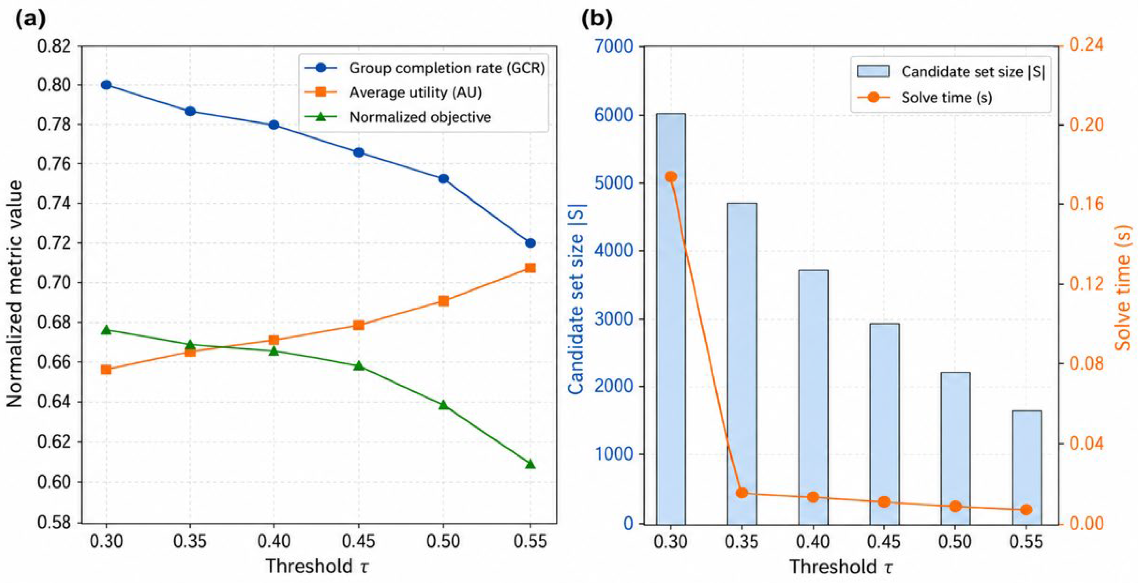
S = { ( i , l ) U × L   |   f i l = 1 ,   w i l τ }
A binary variable x i l is created only for pairs in S . For all pairs outside S , x i l is fixed to zero and is not passed to the solver. This reduction does not change the meaning of the optimization problem; it only removes pairs that are infeasible or below the minimum relevance threshold.
For larger instances, PA-HCGO does not construct a dense user–lot matrix. The implementation stores candidate user–lot pairs as sparse records of the form (user_id, lot_id, utility, cost, and feasibility_flag). User histories, category preferences, and referral lists are also stored as sparse dictionaries or compressed adjacency lists. This design is important because the number of all possible user–lot pairs grows as | U |   | L | , while only a small subset is feasible after budget, capacity, stock, history, and utility threshold filtering. The optimization model is therefore built only on the reduced candidate set S, not on the full Cartesian product U   ×   L .

Illustrative Example of Candidate Set Construction

To make the formulation more transparent, consider a small example with three users, two products, and two active group-buying lots. Let U = { u 1 ,   u 2 ,   u 3 } , P = { p 1 ,   p 2 } , and L = { l 1 ,   l 2 } . Lot l 1 is linked to product p 1 , and lot l 2 is linked to product p 2 . The utility threshold is τ = 0.40 , the activation weight is μ = 0.5 , and each user may join at most one lot, so g i = 1 for all users.
Table 5 gives the lot-level parameters. Lot l 1 already has one participant and requires one more participant to reach its minimum group size. Lot l 2 has no initial participants and requires two new participants. Lot-level parameters in the illustrative PA-HCGO example are shown in Table 5.
Table 6 shows the learned user–lot utilities and the feasibility indicators. A pair is included in the reduced candidate set S only if it is feasible and if its utility is not below the threshold τ = 0.40 .
Construction of the reduced candidate set S . The pair ( u 3 ,   l 1 ) is feasible but excluded because its learned utility is below the threshold (Table 6).
In this example, the reduced candidate set is therefore:
S = { ( u 1 , l 1 ) , ( u 1 , l 2 ) , ( u 2 , l 1 ) , ( u 2 , l 2 ) , ( u 3 , l 2 ) }
The optimization model then selects binary variables only for pairs in S . For example, one feasible solution is to recommend lot l 1 to users u 1 and u 2 . This gives x u 1 l 1 = 1 , x u 2 l 1 = 1 , and y l 1 = 1 because the final number of participants in l 1 becomes 1 + 2 = 3 , which is not lower than q l 1 = 2 . However, this solution does not activate l 2 .
A different feasible solution is to recommend lot l 1 to u 1 and lot l 2 to u 2 and u 3 . In this case, both lots become algorithmically activatable: l 1 reaches 1 + 1 = 2 participants and l 2 reaches 0 + 2 = 2 participants. This example shows why the optimization problem is not equivalent to independent top-N recommendation. The model may assign a user to a slightly lower utility lot if that assignment helps satisfy a group threshold and improves the full objective.
A comparison of two feasible assignment solutions is presented in Table 7. Solution B illustrates how PA-HCGO can prefer a coordinated group activation solution over independent high-utility assignment (Table 7).
With A m a x = 3 , L = 2 , and μ = 0.5 , Solution B also has a higher value of the normalized PA-HCGO objective because it combines higher total assignment utility with activation of both lots. The example illustrates the main logic of the model: learned utility determines the relevance of user–lot pairs, while the optimization layer coordinates these pairs under group-size, capacity, stock, budget, and participation constraints.

4.8. Hybrid Solution Procedure

Using machine learning together with combinatorial optimization follows the general logic of learning-augmented optimization [29,30]. In PA-HCGO, the learned preference layer produces the coefficients w i l , while the optimization layer enforces feasibility and group activation constraints.
The solution mode is selected according to the size of the reduced candidate set S . If the number of candidate pairs is small enough, the exact binary integer program is attempted:
| S | κ
If the number of candidate pairs exceeds the switching threshold, the heuristic mode is used:
| S | > κ
The threshold κ is an empirical operational threshold selected based on validation instances under the same solver, time limit, and hardware settings used in the experiment. In the experiments, the switching threshold equals 2000 candidate pairs: the exact mode is applied to reduced instances with at most 2000 candidate pairs, such as the 50-user/20-lot subproblems of Section 6.5, while larger instances, including P0 with 3743 candidate pairs at the base threshold τ = 0.40 , use the heuristic mode. It is not a theoretical guarantee that every instance with S κ will be solved to optimality. If the exact solver proves optimality within the time limit, the optimal solution is reported. If optimality is not proven within the time limit, the best feasible solution and the solver gap are stored.
For larger reduced instances, PA-HCGO uses a heuristic procedure that is designed to construct a feasible solution for the same objective and constraints as the complete formulation in Section 4.6.8. The heuristic has three stages: activation-oriented initialization, utility-based completion, and bounded local improvement.
For each lot l , the current activation deficit is l :
l = m a x ( 0 ,   q l m l 0 )
A smaller Δ l means that the lot is closer to activation. To combine activation proximity with user relevance, the heuristic computes a lot-priority score:
R l = μ 1 + l + ( 1 μ ) w ¯ l
where w ¯ l is the average learned utility of the best currently feasible candidate users for lot l . Lots with higher R l are considered earlier because they combine a higher probability of threshold completion with stronger user–lot relevance.
After the activation-oriented initialization, the algorithm considers the remaining candidate pairs and adds assignments with positive marginal objective gain, provided that all constraints remain satisfied. The marginal gain of adding pair ( i , l ) is:
Z i l = ( 1 μ ) w i l A m a x + μ y l | L |
where Δ y l = 1 if adding user i makes lot l algorithmically activatable, and Δ y l = 0 otherwise. A local improvement stage then checks feasible add, drop, and swap moves. A move is accepted only if it preserves all constraints and increases the full objective Z .
Algorithm 1 summarizes the complete PA-HCGO solution procedure. The algorithm first constructs the reduced candidate set S , and then selects the exact or heuristic solution mode according to the empirical switching threshold κ . The exact mode solves the binary integer program defined in Section 4.6.8. The heuristic mode constructs a feasible assignment through activation-oriented initialization, utility-based completion, and optional local improvement. Both modes optimize the same objective and use the same feasibility constraints.
Algorithm 1. PA-HCGO solution procedure
Input:
User set U ; lot set L ; product set P ; learned utilities w i l ; feasibility indicators f i l ; initial lot participants m l 0 ; minimum group sizes q l ; lot capacities c l ; product stocks s j ; joining costs a i l ; user spending limits B i ; maximum simultaneous participations g i ; utility threshold τ ; activation weight μ ; exact/heuristic switching threshold κ ; solver time limit T m a x ; and maximum number of local search iterations R m a x .
Output:
Assignment matrix X = ( x i l ) , activation vector Y = ( y l ) , and objective value Z ( X , Y ) .
1. Construct the reduced candidate set:
                                         S = { ( i , l ) U × L | f i l = 1 ,   w i l τ }
2. If S = , return X = 0 , Y = 0 , and Z = 0 .
3. Compute the normalization constant:
                                        A m a x = m a x { 1 ,   m i n ( | S | ,   i U g i ,   l L ( c l m l 0 ) ,   j P s j ) }
4. If | S | κ , submit the binary integer program in Section 4.6.8 to the exact solver with time limit T m a x .
5. If the exact solver proves optimality within T m a x , return the optimal X , Y , and Z ( X , Y ) .
6. If the exact solver does not prove optimality within T m a x , store the best feasible solution and solver gap. If a feasible incumbent exists, use it as the initial solution for the heuristic mode.
7. Initialize X = 0 , Y = 0 , remaining user budgets B i r e m = B i , remaining user participation slots g i r e m = g i , remaining lot capacities r l = c l m l 0 , and remaining product stocks s j r e m = s j .
8. For each lot l L , compute its current deficit:
                                                         l = m a x ( 0 , q l m l 0 )
9. For each lot l L , compute an activation priority score:
                                                         R l = μ 1 + l + ( 1 μ ) w ¯ l
where w ¯ l is the average utility of the best available candidate users for lot l .
10. Sort lots in descending order of R l .
11. For each lot l in the sorted list:
11.1. Select candidate users i with ( i , l ) S , which are sorted by decreasing w i l .
11.2. Add the highest-utility feasible users to lot l while all constraints remain satisfied.
11.3. Stop adding users to l when the lot reaches its activation threshold, reaches capacity, or no feasible candidate remains.
11.4. If
                                                          m l 0 + i U x i l q l
set y l = 1 .
11.5. If lot l does not reach the activation threshold after the tentative additions, set x i l = 0 for all tentative assignments to this lot and restore the corresponding budget, participation slot, capacity, and stock counters.
12. Utility-based completion stage. For each remaining candidate pair ( i , l ) S not yet selected, compute the marginal objective gain:
                                                        Z i l = ( 1 μ ) w i l A m a x + μ y l | L |
where y l = 1 if adding user i makes lot l activatable, and y l = 0 otherwise.
13. Sort remaining candidate pairs by decreasing Z i l .
14. For each remaining candidate pair ( i , l ) :
14.1. If assigning user i to lot l preserves all feasibility constraints and Z i l > 0 , set x i l = 1 .
14.2. Update remaining budget, user participation slots, lot capacity, product stock, and activation status y l .
15. Local improvement stage. Repeat for at most R m a x iterations:
15.1. Generate feasible add, drop, and swap moves over selected and unselected candidate pairs.
15.2. For each move, compute the change in the full objective Z ( X ,   Y ) .
15.3. Apply the best feasible move if it increases Z ( X ,   Y ) .
15.4. Stop if no improving move exists.
16. Recompute each activation variable:
                                                   y l = { 1 ,   i f   m l 0 + i U x i l q l , 0 ,   o t h e r w i s e .
17. Return X , Y , and Z ( X ,   Y ) .
Algorithm 1 uses the same objective and constraints as the complete mathematical formulation. The heuristic part does not define a different optimization problem; it provides a scalable way to construct a feasible solution when the reduced candidate set is too large for exact optimization. The activation-oriented initialization prioritizes lots that are close to their minimum group-size threshold and have sufficiently high utility candidates. The utility-based completion stage then adds assignments with positive marginal objective gain. The local improvement stage checks whether feasible add, drop, or swap moves can further improve the full objective. After each construction round, the heuristic removes assignments in lots that did not reach their activation threshold and returns the freed budget, participation slots, and stock to the candidate pool; this cleanup step enforces the batch assignment constraint and keeps the heuristic solution feasible for the complete formulation in Section 4.6.8.
A local change is accepted only if the new solution stays feasible and increases the objective. The search stops when there is no improvement, or after a set number of iterations.

4.9. Computational Complexity of PA-HCGO

The computational complexity of PA-HCGO depends mainly on the size of the reduced candidate set rather than on the full number of possible user–lot pairs. Let n = | U | be the number of users, m = | L | the number of active lots, h = | P | the number of products, and s = | S | the number of feasible candidate user–lot pairs after pre-reduction.
In the worst case, constructing the candidate set requires checking all pairs in U × L , which gives O ( n m ) . However, the optimization model is not built on the full Cartesian product. It is built only on S . In sparse platform data, this distinction is important because:
s n m
The exact formulation is a binary integer program. It contains one binary assignment variable x i l for each candidate pair ( i , l ) S and one binary activation variable y l for each lot. Therefore, the number of binary variables is:
N v a r = s + m
The number of constraints is linear in the number of candidate pairs, users, lots, products, and observed user–product combinations appearing in S . Let b denote the number of distinct user–product combinations induced by candidate pairs in S . Then, the number of constraints can be summarized as:
N c o n = O ( m + n + h + b + s )
where b n h . The exact formulation is a binary integer program and therefore has exponential worst-case complexity. For this reason, the exact solver is used only for reduced instances that satisfy S κ and only under a fixed time limit.
For larger instances, PA-HCGO uses the heuristic mode. The main operations of the heuristic are candidate sorting, lot-priority sorting, activation-oriented assignment, utility-based completion, and bounded local improvement. Table 8 summarizes the computational complexity of these stages.
The table shows that the practical scalability of PA-HCGO is controlled by s = S , not by the dense product n m . Candidate filtering is therefore not only a preprocessing step but also the main mechanism that keeps the optimization problem computationally manageable. The exact BIP is useful for small, reduced instances and for measuring heuristic quality. The heuristic version is used for larger instances because it avoids solving a dense n × m binary assignment problem.
The bounded local search complexity in Table 8 reflects the prototype implementation used in this study. If all possible pairwise swaps were examined, the local search stage could grow quadratically in s . In the implemented version, the candidate list for local improvement is restricted to feasible add, drop, and swap moves with positive or near-positive marginal value, which gives the practical bound O ( R m a x s ) . This is consistent with the prototype-calibrated scalability experiments reported in Section 6.6.

4.10. Reproducibility and Ethics

For reproducibility, we fix the temporal split boundary, the event weights, the dimension of the latent vectors, the number of graph layers, the regularization coefficients, the utility threshold τ , the weight μ , the threshold κ , the solver time limit, and the random number seeds. Hyperparameters are chosen only on the training and validation sets. The test interval is used only for the final evaluation.
The data are processed in anonymized form. User identifiers are needed only to link tables and are not used as meaningful features. The research set contains no names, phone numbers, e-mail addresses, exact delivery addresses, payment details, or other direct identifiers.
An optimization assignment is not an automatic purchase. In the user application, x i l = 1 means a display priority or a recommendation to join a lot. The final decision stays with the user. This matters both for interpreting the results and for an ethically correct deployment.

4.11. Section Summary

The methodology gives a clear path from prototype data to an optimization solution. Behavioral events are turned into implicit feedback. Matrix factorization forms the base interest model. The social graph refines the user representations. The content component supports cold-start users. The formal lot context model includes discount, fill level, and urgency. However, only the learned product preference score and the static discount attribute were active in the reported experiments; the fill-level and urgency coefficients were fixed at zero because they could not be reliably estimated from the available lot timeline.
The binary model treats products and lots separately. It accounts for the current member count, the minimum threshold, the capacity, the spending limit, the number of simultaneous participations, and the total product stock. The normalized objective allows the study of the trade-off between personalized utility and group completion. To stay computationally usable, PA-HCGO combines pre-filtering, an exact solution for small and medium instances, and a heuristic improvement for large ones.
The next section describes the SmartBuy Connect prototype dataset, the rules for its cleaning and temporal split, and the procedure for building the calibrated test scenarios.

5. Experimental Base and Evaluation Protocol

5.1. Research Questions

The experimental part checks more than the quality of preference prediction. It also checks whether the proposed approach can form feasible groups under threshold, budget, and resource constraints. This setup differs from a standard recommender evaluation. A high-ranking accuracy on its own does not guarantee more successfully formed lots, and it says nothing about the computational usability of the algorithm in a platform setting.
The evaluation is organized around four research questions.
RQ1. Does combining behavioral MF-BPR, content/cold-start scoring, and optional referral information improve transactional intent ranking relative to popularity, matrix factorization, content only, and item neighborhood baselines?
RQ2. Does PA-HCGO give a higher average assignment utility and a larger share of activated lots, compared with independent ranking and a greedy allocation of users?
RQ3. What are the contributions of the content/cold-start component, behavioral MF-BPR, the optional referral-based social signal, and the activation bonus in the PA-HCGO objective?
RQ4. How do the solve time, the gap to the exact optimum, and the quality of the formed groups change as the number of users, products, and active lots grows?
Answering these questions requires three explicitly separated evaluation tracks: observed temporal recommendation testing, a calibrated counterfactual P0 pre-activation experiment, and synthetic S1–S3 scalability testing. This design is referred to as a prototype-calibrated three-track evaluation protocol.

5.2. Data Origin and Limits of Applicability

The experimental base comes from an anonymized export of the SmartBuy Connect prototype, provided as Supplementary File S1 (SmartBuyConnect_Dataset.xlsx). The dataset reflects the logical structure of the application and includes the buyer, seller, product, lot, user event, order, aggregated preference, and referral link entities. The data are used to check the match between the software architecture and the mathematical model, to build implicit feedback, and to calibrate the extended scenarios.
The event and order timestamps (8 January–28 February 2026) are genuine logging timestamps of the SmartBuy Connect prototype, produced during a controlled internal operation session of the platform shortly before manuscript revision; they are not scraped market data and not retrospective reconstructions. Because the prototype was operated in a controlled setting, these records support the calibration and temporal split methodology of this study, but they must not be interpreted as evidence of organic market behavior. The lot window inconsistency described in Section 5.7 is a defect of this prototype export, and it is reported openly rather than corrected post hoc.
The set is not a representative sample of the whole e-commerce user population. It reflects a controlled operation of the prototype, so it does not support direct conclusions about market behavior at industrial scale. This limitation shapes the study design. Prototype observations are used for empirical testing and for assessing the structure of interactions, while computational scalability is studied in the separately described calibrated scenarios.
All user identifiers are anonymized. The research set contains no names, phone numbers, e-mail addresses, exact delivery addresses, payment details, or other direct identifiers. The payment method is a categorical feature and includes no financial data about the payment instrument.

5.3. Structure of the Prototype Dataset

The dataset has eight logically linked tables. Their purpose and size are given in Table 9.
Referential integrity was checked across the key relations between tables. In this export, there were no links to missing users, products, lots, or sellers. All product records link to existing sellers, events link to existing users and products, and orders link to valid users, lots, products, and sellers. This consistency lets the path from a user action to a transactional outcome be reconstructed without joining records by approximate text features.
Because the social component of PA-PREF uses referral links, the referral graph was also diagnosed separately. The referral links table contains 200 directed links among 150 anonymized users. The graph is sparse: the directed density is 0.009, and the undirected density is 0.018 after collapsing reciprocal or duplicate directionality. The average in-degree and out-degree are both 1.33. Twelve users have no referral connection, and the weakly connected structure contains 16 components, with the largest component including 132 users. The total degree distribution is concentrated at low values: 12 users have degree 0, 26 have degree 1, 35 have degree 2, 31 have degree 3, 31 have degree 4, and only 15 users have degree 5 or higher. These values confirm that the referral graph is informative as a prototype signal but too small and sparse for strong claims about social graph learning.
Referral graph diagnostics (Table 10). The graph statistics show that the referral structure is useful as an exploratory social signal but remains too sparse for strong claims about graph-based recommendation.

5.4. Distribution of Behavioral Events

The user events table holds 4000 observations of seven types. The most common event is a product view. The set also includes actions that signal stronger purchase intent, such as joining a lot, moving to checkout, and creating an order. The distribution of events is shown in Figure 3.
As Figure 3b shows, product views account for 2020 of 4000 events, that is, 50.5% of the behavioral log. Search interactions account for 726 observations, lot joins for 589, checkouts for 264, offer sharing for 194, lot creation for 136, and lot leaving for 71. This pattern matches a typical digital commerce funnel, in which top-of-funnel actions are far more frequent than transactional events.
The model does not assume that all events are equally informative. A product view is a weak positive signal. A lot join is a clear intent to participate. A confirmed or completed order is the strongest observed confirmation of a preference. Leaving a lot is read as a negative or weakening signal. The specific event weights are set only on the training and validation parts of the data, which keeps the test set out of the tuning of the implicit feedback transformation.

5.5. Transactional Outcomes

The orders table holds 500 records. Of these, 231 orders are completed, 172 are confirmed, 50 are processing, 35 are cancelled, and 12 are refunded. The distribution is shown in Figure 3c.
Completed and confirmed orders together account for 403 records, that is, 80.6% of the order set. This figure should not be read as a market conversion estimate because the data come from a controlled prototype loop. In this study, order states are used mainly to set the strength of the positive signal and to check the consistency of the interest–participation–checkout–outcome sequence.
The set has four payment methods: card with 246 records, cash on delivery with 92, Kaspi QR with 92, and installment with 70. The payment method can serve as a context feature in behavioral analysis. In the base version of PA-HCGO, it is not included in the objective to avoid mixing group formation with credit or payment scoring.

5.6. Data Preprocessing

Preprocessing is done before the temporal split. The statistics of the transformations, however, are estimated only on the training interval. The procedure includes the following steps:
  • Checking the uniqueness of primary identifiers;
  • Checking referential integrity between tables;
  • Removing exact duplicate events;
  • Converting timestamps to a single time zone;
  • Checking the logical order of lot and order states;
  • Checking that prices, group sizes, and capacities are valid;
  • Encoding categorical features;
  • Building aggregated features only from events available at the prediction moment.
The last step prevents leakage of future information. For example, the completed state cannot be used when computing features for a recommendation made before the corresponding order is finished. Likewise, the final number of lot members is not used as a feature if it was not yet known at the decision moment.
We also check that there are no temporal contradictions. A join event must not happen after the lot closes, and an order date must not precede the registration of the user or the creation of the product. Observations that break these rules are removed or sent for manual review.
Temporal provenance of learned inputs: The exported user preferences table contains one latest aggregate for each observed user–category pair and does not preserve historical versions of previously updated records. The unfiltered full-period table was not used in the main test evaluation.
For the content/cold-start component, an as-of-training-boundary profile was constructed by retaining only user preferences records whose updated_at timestamp was not later than 13 February 2026, which is the end of the training interval. This rule retained 952 of 1415 records and excluded 463 records (32.7%) updated after the training boundary. User–category pairs updated later were treated as unavailable, and no earlier score was imputed because the export does not contain historical versions of those records.
This procedure prevents post-training user–category information from entering the test ranking. It should be interpreted as conservative temporal filtering of the exported profile table rather than as an exact reconstruction of the historical profile state or recomputation from raw training period events. The MF-BPR representations were trained using interactions available through the training boundary. The operational lot utility coefficients were also fitted on the training interval only. Hyperparameters and component weights were selected using the validation interval, while no test-period observations were used for model fitting or parameter selection.

5.7. Lot Timestamp Consistency and Use of Lot Context Features

Because PA-HCGO includes lot-level context variables, the temporal consistency of lot-linked events was checked separately. This check is necessary because fill level and urgency are meaningful only if the state of a lot can be reconstructed at the moment when a user action occurred. If a lot-linked event falls outside the recorded recruitment window of the corresponding lot, it cannot be safely used to estimate time-dependent lot context features.
The consistency check showed that 1060 user events contained a lot identifier. Of these, only 79 events fell within the recorded start–end interval of the corresponding lot, while 981 events were outside that interval. The most plausible explanation is that the prototype export stored the final lot state and not the full history of intermediate lot state changes; an additional time zone conversion issue may also have contributed to the mismatch.
This finding affects how the empirical evidence is interpreted. Events outside the recorded lot window were not used to estimate fill-level, urgency, or other time-dependent lot context effects. They were retained only as user–product interaction signals when the user and product identifiers were valid. In other words, these events contribute to the product preference layer but not to the dynamic lot context layer.
The discount attribute was treated differently because it is a static product–lot attribute and does not require reconstruction of the lot state at a specific decision time. By contrast, fill level and urgency depend on the exact temporal state of the lot and are retained in the formal model but remain inactive in all reported experiments in the current prototype dataset.
Use of lot-linked events after timestamp consistency checking: Table 11 separates records used for product preference estimation from records that can support dynamic lot context features.
This separation prevents temporal leakage and avoids using reconstructed or inconsistent lot states as if they were observed at the decision moment. It also narrows the interpretation of the experimental results: the current evidence validates the preference learning and constrained assignment pipeline more strongly than the dynamic lot context component.

5.8. Temporal Split

A random split of interactions can leak a user’s future actions into the training set. A chronological protocol is therefore used. Let t 1 and t 2 be the boundaries of the training and validation intervals. The training, validation, and test parts are then defined as follows:
D t r a i n = { e D : t e t 1 }
D v a l = { e D : t 1 < t e t 2 }
D t e s t = { e D : t e > t 2 }
The base configuration uses the earliest 70% of events for training, the next 15% for validation, and the last 15% for testing. The boundaries are set by time, not separately for each table. Orders and lot states are matched to the time interval in which the corresponding information becomes available to the platform.
For the cold-start evaluation, a subset of users with fewer than H m i n interactions in the training part are also formed. This subset is analyzed separately from users with enough history because the average quality over the whole set can hide a drop in quality for new users.

5.9. Calibrated Scaling Scenarios

The size of the prototype set is enough to check data connectivity and model behavior for a limited number of users. It is not enough to assess the computational load at platform scale. Calibrated scenarios are therefore added. They keep the observed distributions of categories, prices, discounts, group sizes, event types, and social graph degrees, while the number of entities grows.
The parameters of the synthetic extension are not set arbitrarily. For each numeric or categorical feature, the empirical distribution is estimated on the prototype data, and new observations are then generated while keeping the valid dependencies. For example, lot capacity must be at least the minimum threshold, the order cost must match the product and the quantity, and a social edge must connect existing users.
The experimental scenarios are given in Table 12.
The scaled scenarios are used to assess computational behavior rather than market representativeness. In these scenarios, the main scalability control variable is not only the number of users and lots, but also the density of feasible user–lot pairs after candidate filtering. The implementation therefore measures the number of generated candidate pairs, the size of the reduced optimization problem, the memory use of sparse candidate structures, and the solve time. This distinction is important because a group-buying platform with many users can remain computationally manageable if feasibility and relevance filtering keep the candidate set sparse.
Each scenario also varies the minimum group size, the share of cold-start users, and the density of feasible user–lot pairs. To reduce the effect of random generation, each scenario is repeated at least 20 times with different fixed seed values. The result tables report the mean, the standard deviation, and the 95% confidence interval.
The three evaluation tracks are summarized in the lower part of Figure 2. Observed prototype data are used for temporal recommendation testing. P0 is a calibrated counterfactual pre-activation experiment, and S1–S3 are synthetic scalability tests. These evidence tracks are analyzed separately to avoid presenting counterfactual or synthetic results as observed historical platform outcomes.
The prototype data are used for the temporal evaluation of the recommendation component and for parameter calibration. The scaled scenarios are used mainly to analyze group formation, to compare the exact and heuristic modes, and to measure solve time.

5.10. Compared Methods

To separate the contribution of preference learning from the contribution of constrained optimization, PA-HCGO is compared with methods of different complexity. The baselines are listed in Table 13.
The baseline set was designed to isolate the main functional components of the proposed framework rather than to claim superiority over every modern recommender or optimization method. POP tests the strength of non-personalized popularity ranking. MF-BPR tests latent personalization from implicit feedback. MF-SOC adds a social component to the preference layer. GREEDY tests independent feasible assignment without global coordination. HCGO-STATIC tests the value of constrained group optimization with a fixed utility. ILP-PA provides an exact reference on small instances. PA-HCGO then combines learned utility, feasibility filtering, exact or heuristic optimization, and local improvement. This comparison is component-oriented and system integration-oriented. ITEM-KNN tests whether a local item neighborhood method can explain the observed transactional ranking performance without relying on latent-factor or content-profile integration.
Scope of the baseline comparison (Table 14). The included baselines are selected to isolate the main components of PA-HCGO. Advanced alternatives are identified as future extensions rather than omitted competitors for a broad state-of-the-art benchmark.
This study does not claim that these baselines exhaust the state of the art in recommendation or mathematical optimization. Models such as LightGCN, NGCF, Neural Collaborative Filtering, factorization machines, gradient-boosted ranking, min-cost-flow formulations, Lagrangian relaxation, and commercial-solver warm starts are relevant alternatives. They are discussed as future extensions because the main contribution of this paper is the integration of preference learning and constrained group-buying assignment in the SmartBuy Connect prototype, not a broad benchmark of all possible recommender and optimization techniques.
POP, MF-BPR, and MF-SOC assess the recommendation layer, but they do not guarantee feasible groups. GREEDY meets the basic constraints, yet it does not optimize the group structure globally. HCGO-STATIC shows how much preference learning improves the original combinatorial model. ILP-PA is the reference for small and medium instances, where an exact solution can be found within the time limit.

5.11. Parameter Settings

The base experimental configuration was selected based on the training and validation intervals and then fixed for the final test evaluation. Table 15 reports the main parameter values used in the experiments. The goal of this table is to make explicit which parameters belong to preference learning, cold-start handling, social propagation, context scoring, candidate filtering, optimization, and statistical testing.
The sensitivity analysis focuses on the parameters most likely to change the interpretation of the results: the utility threshold τ , the activation weight parameter μ , the cold-start threshold H m i n , the embedding dimension d , and the exact/heuristic switching threshold κ . Parameters that mainly affect training stability, such as the learning rate and regularization coefficient, were selected based on the validation interval and then held fixed in the final test evaluation.

5.12. Recommendation Quality Metrics

For each user, the test set of relevant products is T i , and the first K positions of the ranked list are R i K . Precision at the first K positions is:
P r e c i s i o n @ K = 1 | U t e s t | i U t e s t | R i K T i | K
Recall at the first K positions are:
R e c a l l @ K = 1 | U t e s t | i U t e s t | R i K T i | | T i |
To account for the position of a relevant item, discounted cumulative gain is used [36]:
D C G @ K i = q = 1 K 2 r e l i q 1 l o g 2 ( q + 1 )
The normalized version is:
N D C G @ K = 1 | U t e s t | i U t e s t D C G @ K i I D C G @ K i
The main configuration evaluates K { 5 , 10 , 20 } . For users with no positive items in the test interval, the ranking metrics are not computed, and the number of excluded users is reported separately.
In the revised reporting, the number of evaluated and excluded users is shown for each relevance definition. For the general engagement target, 148 users had at least one held-out positive item and two users were excluded from top-K metric computation. For the transactional target, 36 users had at least one held-out transactional item and 114 users were excluded because they had no transactional positive item in the test interval.

5.13. Group Formation Metrics

The average utility of the executed assignments is:
A U = i U l L w i l x i l i U l L x i l
If the algorithm makes no assignment, AU is treated as undefined and is not replaced by zero.
The share of activated groups is:
G C R = l L y l | L |
User coverage is the share of participants who received at least one feasible assignment:
U s e r C o v e r a g e = 1 | U | i U I   ( l L x i l > 0 )
To check the correctness of a solution, the share of satisfied constraints is computed:
F e a s i b i l i t y R a t e = 1 V ( X , Y ) V m a x
where V ( X , Y ) is the number of detected violations of budget, capacity, the activation threshold, product stock, and participation limits, and V m a x is the number of checked constraints. For an exact and a correctly implemented hybrid algorithm, the expected value is 1.
We also record the number of activated lots, the number of assigned users, the average member deficit before and after optimization, and the share of lots that stayed below the activation threshold.

5.14. Computational Efficiency Metrics

In the exact solution comparison, the objective value used in the gap calculation is the same normalized PA-HCGO objective as in Equation (35). For a subproblem r, let Z r I L P denote the proven optimal objective value obtained by ILP-PA and let Z r H denote the objective value obtained by the PA-HCGO heuristic on the same reduced candidate set. The relative heuristic gap is computed as:
G a p r = Z r I L P Z r H m a x ( | Z r I L P | , ε )
where ε = 10 9 is used only to avoid division by zero. The reported average gap is the arithmetic mean of G a p r over the 20 exact comparison subproblems.
Run time is measured from the moment the prepared problem is passed to the optimization module to the moment a feasible solution is obtained. The pre-filtering time, the exact or heuristic optimization time, and the total latency are recorded separately. For each scenario, the median, the 95th percentile, and the maximum observed time are reported.
The exact solver has a single time limit. If a proven optimum is not found, the best feasible value, the solver lower or upper bound, and the corresponding solver gap are stored. Such cases must not be read as an exact optimum (Table 16). The reported v1.2.0 exact comparison runs were solved using scipy.optimize.milp with the HiGHS backend [37]. The reproducibility package also supports OR-Tools CP-SAT [38] as an optional backend, but the numerical results reported in this manuscript correspond to the recorded SciPy/HiGHS runs.

5.15. Ablation and Sensitivity Analysis Protocol

The recommendation layer ablation includes:
  • Without the referral-based social component: the model uses behavioral MF-BPR and content/cold-start scores;
  • Without the content/cold-start component: the model uses only the behavioral MF-BPR and referral-based social scores;
  • Without the behavioral MF-BPR component: the model uses the referral-based social and content/cold-start scores;
  • Popularity-only preference scoring.
The optimization layer sensitivity separately compares μ = 0 and μ = 0.4 to evaluate the activation bonus.
The change in any metric M relative to the full model is:
Δ M = M f u l l M a b l a t e d
The sensitivity analysis covers μ , τ , H m i n , the embedding dimension, the number of graph layers, and the threshold that switches between the exact and heuristic modes. When one parameter is analyzed, the others are fixed at the values chosen based on the validation set.

5.16. Statistical Testing

Each calibrated configuration is run at least 20 times. To compare two methods, paired results from the same scenario realizations are used. The main uncertainty estimate uses a non-parametric bootstrap with 10,000 resamples. A difference is treated as statistically significant if the 95% confidence interval for the paired difference does not include zero. The method follows the non-parametric bootstrap estimate [39].
Besides significance, the effect size is reported. This matters because, with many repetitions, even a small difference can be statistically significant yet have no practical value for the platform. No multiplicity correction was applied to the paired bootstrap comparisons. Given the exploratory, prototype-calibrated framing, we designate PA-PREF versus POP/MF-BPR/MF-SOC (recommendation layer) and PA-HCGO versus GREEDY (group formation) as the primary comparisons. All remaining paired comparisons are reported descriptively and should not be read as confirmatory family-wise tests.

5.17. Section Summary

The protocol separates three aspects of quality: the accuracy of preference learning, the effectiveness of forming feasible groups, and computational usability. The prototype dataset is used for the temporal evaluation of the recommendation component and for empirical calibration. The scaled scenarios allow the study of the algorithm under a load that is not yet reachable at the current stage of operation.
The comparison with popularity ranking, matrix factorization, greedy assignment, the static HCGO model, and the exact ILP shows how much improvement comes from preference learning and how much comes from global optimization. The ablation and sensitivity analyses are needed to show that the improvement is not the result of a single well-chosen parameter.
The next section presents the actual experimental results: ranking quality, group completion, the comparison with the exact solution, the computational latency, and the contribution of the individual PA-HCGO components.

6. Results

This section presents the results of the actual computational experiment, run on a re-loaded SmartBuy Connect dataset. The evaluation has two levels. First, we study the ranking quality of products on chronologically held-out interactions and on transactional events. Then, we analyze the ability of the optimization layer to form feasible buyer groups in the prototype and in the scaled scenarios. The reported results are grouped by the type of evidence used to obtain them. Recommendation metrics are computed from the observed temporal test split of the prototype dataset. The P0 group activation results are computed in a calibrated counterfactual pre-activation scenario constructed from the prototype lot parameters. The S1–S3 results are obtained from synthetic scalability scenarios generated from prototype-calibrated distributions. This separation is used throughout the section to avoid interpreting calibrated or synthetic scalability results as observed historical platform outcomes.

6.1. Data Checking and Preparation Results

The initial check confirmed the uniqueness of the identifiers for sellers, products, users, lots, events, orders, and referral links. There were no missing links between products and sellers, between orders and users, or between orders, lots, and the corresponding products. All 500 orders matched the seller listed in the card of the corresponding product.
The lot timestamp consistency check described in Section 5.7 confirmed that only 79 of 1060 lot-linked events fell within the recorded start–end interval of the corresponding lot. The remaining 981 lot-linked events were excluded from time-dependent lot context estimation and retained only as user–product preference signals when their user and product identifiers were valid. Therefore, the results below should be interpreted as a stronger validation of the preference learning and constrained assignment pipeline than of the dynamic lot context component.
The resulting data-quality checks and temporal-split counts are summarized in Table 17.
The global split boundaries were 13 February 2026 for the end of the training interval and 20 February 2026 for the end of the validation interval. Products that a user interacted with during training were removed from the candidate list at test time. This makes the task stricter because the model has to find items that are new to the user rather than re-rank items already seen.

6.2. Quality of the Recommendation Layer

The matrix model was trained in five independent runs with different random seeds. The configuration used 16 latent factors, 60 epochs of pairwise training, an initial learning rate of 0.02, and a regularization coefficient of 0.002. The final MF-BPR score was the average of five prediction matrices. The weights of the full PA-PREF model were chosen only on the validation transactional set. The best combination used 0.4 of the behavioral MF-BPR score, 0.1 of the social component, and 0.5 of the content user–category profile.
The results are reported separately for two definitions of relevance. In the diagnostic task of general engagement, all positive actions were treated as relevant, including views and search. In the main transactional task, only new products linked to orders in the completed, confirmed, or processing states were counted. This split is needed because a frequent product view is not the same as purchase intent.
For the general engagement evaluation, 148 users had at least one relevant item in the test interval, while two users were excluded from top-K metrics because they had no test positives. For the transactional intent evaluation, 36 users had at least one held-out transactional item, while 114 users were excluded from top-K metrics because they had no transactional positive in the test interval. The transactional results describe a small subset of users with observed purchase intent outcomes.
The ranking results for both relevance definitions are reported in Table 18.
For general engagement, the highest NDCG@10 came from the popularity approach (0.0802). PA-PREF reached NDCG@10 = 0.0515 and did not beat this baseline. ITEM-KNN obtained NDCG@10 = 0.0545, while CONTENT obtained 0.0524. None of the personalized models exceeded POP at 0.0802 for the general engagement target. This indicates that views and searches in the prototype set are largely driven by overall product popularity rather than by stable individual latent preferences. The set therefore gives no basis to claim that a complex model improves the ranking of all types of user activity.
This distinction is important for the interpretation of PA-PREF. In the current prototype dataset, product views and searches are frequent and appear to be strongly driven by overall item popularity. Therefore, general engagement is not the strongest validation target for the hybrid preference model. The more appropriate target is transactional intent, where the positive signal is closer to an actual purchase decision. For this reason, this paper treats the transactional evaluation as the main evidence for the preference layer and treats the general engagement result as a negative or boundary condition.
The main transactional results use the as-of-training-boundary user–category profiles described in Section 5.6. PA-PREF achieved Precision@10 = 0.0389, Recall@10 = 0.3611, NDCG@10 = 0.1319, and Hit rate@10 = 0.3889. The corresponding content-only model achieved Precision@10 = 0.0278, Recall@10 = 0.2639, NDCG@10 = 0.1034, and Hit rate@10 = 0.2778.
On NDCG@10, the absolute difference between PA-PREF and POP was 0.1061, the difference between PA-PREF and MF-BPR was 0.1053, the difference between PA-PREF and MF-SOC was 0.1167, and the difference between PA-PREF and the content-only model was 0.0285. A paired non-parametric bootstrap with 10,000 resamples produced a 95% confidence interval of [0.0475, 0.1656] for PA-PREF versus POP, [0.0455, 0.1681] for PA-PREF versus MF-BPR, and [0.0643, 0.1744] for PA-PREF versus MF-SOC. For PA-PREF versus the content-only model, the interval was [−0.0220, 0.0800]. The PA-PREF versus ITEM-KNN interval was [0.0513, 0.1529]. PA-PREF remained statistically stronger than the popularity and matrix factorization baselines, but its advantage over the content-only model was not statistically separable at the 95% level.
A cosine ITEM-KNN baseline (50 neighbors) was also evaluated on the transactional target. It reached NDCG@10 = 0.0323 and Hit rate@10 = 0.1111, which is comparable to POP and MF-BPR and far below both the content model and PA-PREF, confirming that an item neighborhood baseline does not explain the transactional advantage of the hybrid preference layer.
Figure 4b shows that the main gain of PA-PREF comes not only from a better position of the relevant product, but also from a larger share of users for whom at least one transactionally relevant item entered the top ten recommendations. At the same time, the transactional test set has 36 users, so the effect should be treated as preliminary and should be rechecked once more real orders accumulate.

6.3. Group Formation in the Prototype Scenario

Scenario P0 used 150 users and 150 lots. The minimum size, capacity, price, and discount parameters were taken from the prototype set. Because the stored current_participants values reflected the final state rather than an intermediate one, and already met the minimum threshold in every lot, a pre-activation point was reconstructed for the experiment. The initial member count was set below the threshold, and the average deficit was about half the minimum group size. Formally, the initial participant count of each lot was set to the floor of one half of its minimum group size, so the initial activation deficit equals about one half of the minimum group size for every lot; this deterministic 50–deficit rule is a neutral midpoint between an almost complete and an almost empty lot state. This is a calibrated counterfactual scenario, not a reconstruction of the actual sequence of joins.
It is important to emphasize that P0 is not an observed historical platform state. The exported lot table contains final lot states, and all 150 lots already satisfy current_participants ≥ min_participants. Therefore, the experiment constructs a counterfactual pre-activation state in order to evaluate how alternative allocation rules behave before group thresholds are reached. The resulting comparison, including the 117 versus 85 activated lots result, should be read as evidence of algorithmic behavior under a calibrated pre-activation setting, not as a measured historical increase in completed real platform lots.
In the base 50–deficit setting, GREEDY, HCGO-STATIC, and PA-HCGO produced 405, 403, and 396 assignments, respectively. These correspond to averages of 2.70, 2.69, and 2.64 assignments per user and remain consistent with the participation cap of three lots per user. The same budget, participation cap, joining cost, capacity, and stock rules were applied to all methods.
To ensure reproducibility of the counterfactual P0 experiment, the joining cost a i l was set equal to the discounted price of the product linked to lot l . Because the prototype users table does not contain user-specific budget or participation cap fields, the experimental spending limit was fixed at B i = 40,000 monetary units and the participation cap at g i = 3 lots for every user. The initial participant count was defined as m l 0 = q l / 2 in the base 50–deficit setting. These rules were applied unchanged to GREEDY, HCGO-STATIC, and PA-HCGO.
To check that the P0 comparison was not an artifact of the 50–deficit rule, the experiment was repeated with initial deficits of 25%, 50%, and 75% of the minimum group size. GREEDY activated 86, 85, and 67 lots, respectively. HCGO-STATIC activated 123, 122, and 104 lots, and PA-HCGO activated 122, 117, and 102 lots. PA-HCGO exceeded GREEDY by 36, 32, and 35 activated lots across the three settings. A paired bootstrap over lots with 10,000 resamples produced a 95% confidence interval of [14.67, 28.00] percentage points for the PA-HCGO versus GREEDY GCR difference in the base 50–deficit setting. The resampling unit was the individual lot within the single constructed P0 scenario. Therefore, this confidence interval reflects within-scenario heterogeneity of the PA-HCGO versus GREEDY effect across lots rather than sampling uncertainty over a real platform population. The 25%, 50%, and 75% initial-deficit analysis is treated as the primary robustness check for the counterfactual P0 comparison.
GREEDY achieved the highest average assignment utility, A U = 0.6841 , because it selected high-utility pairs independently. However, it activated only 85 of 150 lots, corresponding to G C R = 0.5667 . HCGO-STATIC achieved the highest group completion rate, activating 122 lots, but its average utility was only 0.5632. PA-HCGO activated 117 lots while maintaining A U = 0.6710 . Relative to HCGO-STATIC, PA-HCGO increased average assignment utility by 0.1078 and the normalized objective by approximately 6.10%. All three solutions satisfied the modeled budget, capacity, stock, participation, and activation constraints.
Table 19 should be read as a trade-off rather than as dominance of one method across all metrics. GREEDY achieved the highest AU because it selected high-utility pairs independently and did not attempt to coordinate users across lot thresholds. This local strategy, however, activated only 85 of 150 lots. HCGO-STATIC and PA-HCGO shifted part of the assignment mass toward threshold completion, which lowered AU relative to GREEDY but substantially increased GCR. PA-HCGO therefore improves the balance between relevance and group activation; it does not dominate GREEDY on average assignment utility alone.

6.4. Scaled Scenario Results

Scenarios S1–S3 were generated by resampling the empirical profiles of users, product categories, prices, discounts, and lot parameters, with a small random perturbation added to the utility scores. Each scenario ran 20 times, with the same realizations for the compared methods. Table 20 reports the means and the standard deviations.
The S1–S3 scenarios are synthetic scalability tests. They preserve selected empirical distributions from the prototype dataset, including product categories, prices, discounts, group-size parameters, and feasible pair sparsity, but they do not simulate strategic user behavior, seller-side reactions, market competition, or real acceptance of recommendations. Their purpose is to test computational scalability and robustness of the optimization procedure, not to claim business effectiveness at platform scale.
In S1, PA-HCGO increased GCR over GREEDY by 6.00 percentage points. The paired 95% confidence interval was [4.92, 7.08] percentage points. AU decreased by 0.0079, while the normalized objective increased by 0.0235. Compared with HCGO-STATIC, PA-HCGO achieved almost the same GCR but increased AU by 0.1741 and the objective by 0.0733.
In S2, PA-HCGO increased GCR over GREEDY by 6.69 percentage points, with a paired 95% confidence interval of [6.03, 7.34] percentage points. AU decreased by 0.0080 relative to GREEDY, while the objective increased by 0.0256. HCGO-STATIC achieved nearly the same GCR as PA-HCGO, but its AU was lower by 0.1967, and its objective was lower by 0.0850.
In S3, the GCR difference narrowed because the available user pool substantially exceeded the aggregate activation deficit. PA-HCGO achieved GCR = 0.8229, compared with 0.8108 for GREEDY and 0.8227 for HCGO-STATIC. The paired PA-HCGO versus GREEDY difference was approximately 1.20 percentage points, with a 95% confidence interval of [1.02, 1.38]. PA-HCGO and HCGO-STATIC therefore achieved almost identical group completion, but PA-HCGO produced substantially higher assignment utility, 0.8441 versus 0.5595. This indicates that, in the high-load scenario, learned utility mainly influences which users are selected rather than how many lots can be activated.
A joint reading of the panels of Figure 5 shows that GREEDY mostly optimizes the local quality of a single pair, while HCGO-STATIC and PA-HCGO reallocate part of the users to reach the activation thresholds. PA-HCGO takes a middle position. It keeps almost the same level of group completion as the static combinatorial model, but it consistently raises the utility of the executed assignments.

6.5. Comparison with the Exact Solution

The exact solution comparison was conducted on 20 subproblems, each containing 50 users and 20 lots. The subproblems were sampled from the same calibrated distribution as the corresponding PA-HCGO experiment. For each subproblem, the same candidate filtering procedure was applied before both ILP-PA and PA-HCGO were run. This means that the exact and heuristic methods were compared on the same reduced feasible pair set rather than on different search spaces. The objective value used in the comparison was the same normalized PA-HCGO objective defined in Equation (35) and used in the complete formulation in Equation (52). In every reported run, the exact solver finished with a proven optimum within the specified time limit. On the same reduced candidate sets, the PA-HCGO heuristic was 20.0 times faster on average, based on the per-instance exact-to-heuristic solve-time ratios summarized in Figure 6b. The comparison with the hybrid heuristic is given in Table 21.
All 20 reported exact runs reached proven optimality with the SciPy/HiGHS backend. The PA-HCGO heuristic had a mean relative objective gap of 3.16% with a standard deviation of 2.43%. The mean of the per-instance exact-to-heuristic time ratios was 20.0×, while the ratio of the mean solve times was approximately 20.84×. These results characterize the tested 50-user/20-lot subproblems and should not be interpreted as a universal approximation or speed guarantee.

6.6. Computational Scalability

The mean PA-HCGO solve time was 0.0986 s in S1, 0.4453 s in S2, and 4.7174 s in S3. For S3, the 95th-percentile time was 4.8417 s, and the maximum observed time was 4.9218 s. HCGO-STATIC had a comparable time because both methods use the same activation-oriented assignment structure and differ mainly in the utility matrix. GREEDY remained faster but achieved a lower group completion rate.
The main reason for this scalability pattern is the sparse construction of the candidate set. PA-HCGO does not optimize over all possible user–lot pairs. It first removes pairs that violate feasibility rules or fall below the utility threshold, and then passes only the reduced candidate set to the exact or heuristic optimization module. Thus, the intermediate data structures scale with | S | rather than with the full Cartesian product size | U | | L | . This is the practical mechanism that allows the method to be tested on the S3 scenario with 5000 users and 1000 lots in the prototype implementation.
Figure 6. Computational performance of PA-HCGO: (a) mean solve time of GREEDY, HCGO-STATIC, and PA-HCGO in S1–S3; (b) mean and 95th-percentile solve times of ILP-PA and PA-HCGO on the 20 exact comparison subproblems.
Information 17 00768 g006
The regenerated experiments were executed in a containerized Linux 6.12.13 x86_64 environment with Python 3.13.5, five allocated virtual CPU cores on an Intel Xeon Platinum 8573C host, and approximately 5.9 GiB of available RAM. The software stack included SciPy 1.17.0 [37], NumPy 2.3.5 [40], scikit-learn 1.8.0 [41], and Numba 0.65.1 [42]. The reported exact comparison outputs used the SciPy/HiGHS backend. Absolute time values are environment-dependent and should not be interpreted as an industrial service-level guarantee.

6.7. Ablation and Sensitivity Analysis Results

The ablation results show that the content/cold-start component remains the dominant contributor to transactional ranking quality. Removing it reduces NDCG@10 from 0.1319 to 0.0153, corresponding to an 88.4% decrease. Removing the behavioral MF component reduces NDCG@10 to 0.1202, an 8.9% decrease. By contrast, removing the referral-based social component increases NDCG@10 from 0.1319 to 0.1403. This 6.3% increase should not be interpreted as evidence that removing the social component is generally beneficial. On the small 36-user transactional subset, it shows that the referral signal provides no confirmed positive contribution and may introduce additional noise.
The contribution of the individual preference-model components is summarized in Table 22.
The comparison with MF-SOC also supports a cautious interpretation of the social component. Although PA-PREF achieved a higher transactional NDCG@10 than the content-only model, the bootstrap confidence interval for that paired difference included zero, while the differences over POP, MF-BPR, and MF-SOC were confirmed. Therefore, the current data do not support a statistically robust claim that the collaborative and social additions improve on the dominant content/cold-start component.
To evaluate the activation bonus, 10 additional exact subproblems with 40 users and 15 lots were solved for μ = 0 and μ = 0.4 . At μ = 0 , mean GCR was 0.7533 ± 0.1118 and mean AU was 0.5967 ± 0.0240 . At μ = 0.4 , mean GCR increased to 0.7733 ± 0.1083 , while AU remained nearly unchanged at 0.5964 ± 0.0242 . Thus, the activation bonus increased GCR by approximately 2.00 percentage points in these exact subproblems without a meaningful reduction in assignment utility.
Sensitivity to the feasibility threshold is shown in Figure 7.
As τ increased from 0.30 to 0.55, the reduced candidate set decreased from 6014 to 1686 pairs, and mean solve time decreased from 0.1821 s to 0.0076 s. At the same time, AU increased from 0.6573 to 0.7076, whereas GCR decreased from 0.8000 to 0.7200. The normalized objective was highest at τ = 0.30 , with a value of 0.6758. The base value τ = 0.40 produced an objective of 0.6663 and was retained as a managerial compromise that reduces candidate volume and recommendation intrusiveness while preserving a comparatively high group completion rate.
To examine cross-method robustness at the objective-preferred threshold, GREEDY, HCGO-STATIC, and PA-HCGO were additionally rerun for P0 and for all 20 fixed seeds of S1–S3 using τ = 0.30 . PA-HCGO retained the highest normalized objective in every evaluated setting: 0.6758 in P0, 0.6752 in S1, 0.6907 in S2, and 0.7317 in S3. In S1–S3, the complete objective ordering remained PA-HCGO > GREEDY > HCGO-STATIC, which is identical to the ordering obtained at τ = 0.40 . In P0, PA-HCGO also remained first, but the two baseline methods exchanged positions: at τ = 0.30 , GREEDY achieved an objective of 0.6020 and HCGO-STATIC achieved 0.5929, whereas at τ = 0.40 , HCGO-STATIC achieved 0.6280 and GREEDY achieved 0.5961. The robustness analysis confirms the threshold stability of the principal conclusion that PA-HCGO provides the highest normalized objective, although the complete baseline ordering is not invariant in P0.
The sensitivity analysis also confirms that the model is most sensitive to parameters that directly change the candidate set or the balance between relevance and group activation. The utility threshold τ affects the number of feasible user–lot pairs, solve time, AU, and GCR. The activation weight μ changes the trade-off between selecting high-utility assignments and completing more groups. The cold-start threshold H m i n affects how long a user remains primarily represented by content/category features before collaborative history is trusted. By contrast, small changes in the latent dimension d and regularization coefficient mainly affect ranking stability and have a weaker influence on group activation metrics after candidate filtering.
A one-dimensional sensitivity sweep was also run for the three preference layer parameters flagged as potentially influential, with all other parameters fixed at their base values. Transactional NDCG@10 was 0.1319 for all tested cold-start thresholds in {3, 5, 8}, because most users accumulate more than eight training interactions and the accumulated history coefficient saturates. The threshold matters only for genuinely short-history users. For the latent dimension, NDCG@10 was 0.1567, 0.1319, and 0.1350 for dimensions 8, 16, and 32, and for the temporal decay coefficient it was 0.1358, 0.1319, and 0.1319 for values of 0.01, 0.05, and 0.10 per day. NDCG@10 therefore varies by less than 0.03 across the tested grids, and the base configuration lies within the plateau of each sweep, which supports the claim that the reported transactional result is not an artifact of a single parameter choice.
As a provenance diagnostic, we also evaluated the model using the unfiltered full-period user preferences export. This diagnostic variant produced PA-PREF NDCG@10 = 0.1330, compared with 0.1319 under the main as-of-training-boundary protocol. The small numerical difference indicates stability of the ranking result. However, the unfiltered value is not used as headline evidence because the full export contains user–category records updated after the training boundary.

6.8. Answers to the Research Questions

RQ1. Combining behavioral, social, and content signals did not improve general engagement ranking over the popularity method. For general engagement, POP obtained the highest NDCG@10, while PA-PREF performed lower. The hybrid preference model gave its best result only for the transactional target, where PA-PREF achieved the highest Recall@10, NDCG@10, and Hit rate@10. The evidence supports the usefulness of PA-PREF for transactional intent prediction, but not a claim of general superiority across all user–activity types.
RQ2. PA-HCGO increased the share of activated lots relative to independent greedy assignment. In P0, the difference was 21.33 percentage points. In S1 and S2, the differences were 6.00 and 6.69 percentage points, respectively, while in S3 the paired difference was approximately 1.20 percentage points. Compared with HCGO-STATIC, the main advantage of PA-HCGO was higher assignment utility and a higher normalized objective rather than a substantially higher GCR.
RQ3. The content/cold-start fallback made the largest contribution to the recommendation layer: removing it reduced transactional NDCG@10 from 0.1319 to 0.0153. The behavioral MF component made a moderate positive contribution (−8.9% in NDCG@10 when removed). The referral-based social component showed no confirmed positive contribution: removing it left NDCG@10 essentially unchanged (+6.3%, within the noise of the 36-user transactional subset), and the paired bootstrap comparison with the content-only model included zero. The activation bonus increased mean GCR by approximately 2.00 percentage points on the exact subproblems while leaving AU almost unchanged.
RQ4. On the small exact comparison subproblems, PA-HCGO had a mean relative objective gap of 3.16% and was 20.0 times faster on average according to the per-instance solve-time ratios. In S3, with 5000 users and 1000 lots, the mean solve time was 4.7174 s and the 95th-percentile time was 4.8417 s. These results support computational feasibility in the tested prototype environment but do not constitute an industrial service-level guarantee.

6.9. Section Summary

The experiment showed that the main advantage of PA-HCGO is the coordination of collective demand. Choosing the most useful pairs independently gives high local relevance, but it fragments users across incomplete lots. Group optimization raises the share of activated lots substantially, and the learned user–lot utility improves the assignment quality over the static combinatorial model.
At the same time, the results do not confirm an unconditional advantage of every component. The popularity method stayed the strongest for general engagement, the referral-based social signal showed no confirmed positive contribution, and the temporal mismatch of a large part of the lot events limited the test of the dynamic context. These points should appear in the discussion as the limits of the evidence, not be hidden behind averaged figures. The next section compares the results with the original research gap and analyzes the theoretical and practical implications, the threats to validity, and the directions for further work.

7. Discussion

The results are not uniformly positive across all metrics, and this is one of the central findings of this study. For general user engagement, the popularity baseline was stronger than the more complex preference models. This means that, in the current prototype dataset, views and searches are explained better by aggregate item popularity than by individualized preference modeling. The advantage of PA-PREF appeared mainly for stronger transactional events linked to completed, confirmed, or processing orders. The correct interpretation is not that PA-PREF is a universally superior recommender, but that it is more useful for transactional intent prediction under the current data conditions.

7.1. Interpreting the Results Against the Research Gap

Section 2 identified a methodological gap between three groups of work: recommender systems, group-buying models, and combinatorial optimization. Recommender models can score a user’s interest, but they do not guarantee that a group threshold, a budget, or a capacity limit is met. Optimization models handle constraints strictly, but they often assume that the utility of a user–product pair is already known. PA-HCGO joins these levels. The learned user–lot utility becomes the input to a binary optimization problem, and the optimization result returns to the platform as a feasible group decision.
The experiment confirms the practical value of this link. The greedy algorithm chose pairs with high individual utility, but it spread users across lots in a fragmented way, so a large share of groups did not reach the activation threshold. This is clearest in the prototype scenario P0, where GREEDY activated 85 of 150 lots, while PA-HCGO activated 117. A locally relevant recommendation is therefore not always a good platform decision. For group buying, it is not enough to predict interest. Demand also must be coordinated.
At the same time, the preference learning evidence must be interpreted narrowly. The hybrid preference layer did not dominate the popularity baseline in general engagement ranking. Its value appears when the target is closer to actual transactional intent. This distinction refines the research gap addressed by this paper: the problem is not merely to improve all product ranking tasks, but to generate utility scores that are useful for downstream constrained group formation and purchase intent-oriented assignment.
The comparison of PA-HCGO with HCGO-STATIC shows the other side of the problem. Static optimization can complete groups effectively, but its assignments are less personalized. In the prototype scenario, PA-HCGO reached a higher average assignment utility and a higher objective value. This supports the initial hypothesis that a static utility limits the adaptivity of the model and should be replaced by data-driven utility scores.

7.2. Theoretical Contribution

The theoretical contribution is to extend the group-buying assignment problem beyond classic product ranking and beyond pure optimization. The proposed model treats group buying as a two-level task. First, the likely utility of a user–lot pair is scored. Then, this score is used in constrained optimization. This lets the recommendation score be seen not as a result, but as a parameter of a downstream decision model.
The contribution should be interpreted as a system-level and formulation-level contribution rather than as a claim of algorithmic dominance over all state-of-the-art recommenders or solvers. The preference layer relies on established implicit feedback and graph-based principles, and the optimization layer relies on binary assignment and hybrid heuristic ideas. The novelty lies in how these components are joined for the specific group-buying setting: the learned utility is not the final output, but a coefficient in a feasibility-preserving assignment model that accounts for lot thresholds, capacity, stock, budget, and multi-group participation.
The social/referral layer is not presented as an independently validated graph learning contribution. In the current prototype, the referral graph is too small and sparse for such a claim. Its role is to demonstrate how social signals can be incorporated into the user–lot utility framework, while stronger validation of graph-based social influence requires a larger referral network and a longer interaction history.
This study also extends the optimization-oriented view of group buying. Prior work on group-buying-based combinatorial reverse auctions has shown that coordinated group buying can improve performance and computational efficiency compared with independent procurement models. The present study transfers this coordination logic to a consumer-facing digital commerce platform. In PA-HCGO, the coordination object is not a bundle of procurement bids, but a set of user–lot recommendation assignments. This shift requires preference learning, feasibility filtering, and activation-aware assignment to be combined in one decision framework.
The first contribution is the formalization of controlled multi-group participation. A user may be interested in several lots, but participation is limited by the budget, the number of allowed groups, and the product terms. This is closer to the real behavior of e-commerce users than a model that lets each user join only one group.
The second contribution is the separation of products and lots. In earlier simplified formulations, one product is often identified with one group. In a more realistic platform architecture, one product can have several active lots that differ in start time, capacity, fill level, and participation context. The introduced set of lots accounts for such cases correctly.
The third contribution is the normalized multi-criteria objective. The model is not reduced to maximizing the number of groups alone or the individual utility alone. The coefficient μ controls the trade-off between user relevance and the platform goal of completing deals. The sensitivity analysis showed that this trade-off is practically meaningful: raising the utility threshold increases the average relevance of the assignments but lowers the share of activated groups.
The fourth contribution is the prototype-calibrated validation strategy. Unlike a fully synthetic evaluation, the parameters and the structure of the scenarios were tied to the exported SmartBuy Connect dataset. This is not an industrial validation, but it raises applied credibility compared with abstract data generation that has no link to a real platform.

7.3. Practical Relevance for a Digital Platform

In practice, PA-HCGO can serve as the intelligent core for managing group buying. In a live platform, the result x i l = 1 should not force the user to buy. It should be read as a display priority, a recommendation to join a lot, or a signal for a platform incentive mechanism. The final participation maintains the user’s choice.
For the buyer, the practical effect is less information overload. Instead of browsing many lots, the system can show the groups that both match the user’s interests and have a high chance of being completed. For the seller, the effect is more predictable demand aggregation. The algorithm helps not only to gather product views, but to bring more lots to the minimum threshold. For the platform operator, PA-HCGO improves the manageability of the ecosystem because it allows a balance between user relevance, group completion, and computational cost.
Table 23 organizes the practical implications of the results for the main platform participants.

7.4. Architectural and Deployment Implications

The results support keeping PA-HCGO as a separate decision service. Such a service should receive current data on users, lots, products, orders, and referral links, form the candidate set, compute the utility, and return a list of priority assignments. Separating the optimization core from the buyer and seller interfaces lowers the technical risk. The algorithm can be updated, tested, and compared with alternatives without a full rework of the application.
For deployment, two-time regimes should be distinguished. Updating the embeddings and the preference model can be done in batches; for example, daily or after enough events accumulate. The optimization of active lots should run more often because the state of the lots changes with each join. This decoupled architecture combines relatively heavy training with fast operational computation.
The mean PA-HCGO solve time in the largest scenario S3 was 4.7174 s, and the 95th-percentile time was 4.8417 s for the sparse candidate set. These values support computational feasibility at the prototype and laboratory level. Industrial deployment, however, will require separate load testing, including concurrent requests, competing lot state updates, fault tolerance, candidate set caching, and latency control under peak demand.

7.5. Interpreting the Individual Model Components

The ablation analysis shows that the current preference layer is not driven equally by all components. The content/cold-start component is the dominant contributor to transactional ranking quality. This is expected at an early prototype stage, where order history is limited and categorical preferences provide a more stable signal than sparse collaborative interactions. The behavioral matrix factorization component adds a moderate contribution. The referral-based social component has the weakest empirical support: removing it does not reduce transactional NDCG@10, and the full blend is not statistically separable from the content-only model at the 95% level. Therefore, the social component should be interpreted as a preliminary architectural extension rather than as a confirmed major driver of PA-PREF performance.
The threshold τ is one of the key controllable parameters. As it grows, the average assignment utility rises, but the number of candidate pairs and GCR fall. The utility threshold is therefore not a technical setting but a managerial parameter of the platform. A lower τ suits a strategy that maximizes group completion. A higher τ suits a strategy that raises user relevance and lowers the risk of intrusive recommendations.

7.6. Threats to Validity

Despite the positive results, this study has several limitations that must be stated clearly. It is important to identify not only the gains in the metrics, but also the limits of applicability of the experiment. The main threats to validity and the corresponding mitigation strategies are summarized in Table 24.
The key internal validity threat concerns the temporal consistency of lot-linked data. Because only 79 of 1060 lot-linked events fell inside the recorded recruitment window of the corresponding lot, the current dataset does not provide sufficient evidence to validate dynamic lot context effects such as fill level and urgency as fully observed time-dependent features. For this reason, inconsistent lot-linked events were excluded from dynamic context estimation and used only as user–product interest signals when their identifiers were valid. This decision reduces the risk of temporal leakage, but it also means that the empirical support for the lot context component is limited. A future version of the platform must log the full event-level lot timeline, including lot creation, participant count changes, notifications, price changes, and closure events.
The second threat concerns the size of the transactional test set. PA-PREF showed a clear advantage on the transactional metrics, but the number of users with such events in the test is limited. The results should therefore be treated as preliminary experimental evidence, not as final proof of commercial value.

7.7. From a Static to a Learned User–Lot Utility

The key difference between the proposed approach and a static combinatorial formulation is the preference learning layer, which changes the role of the utility matrix. In the static version (HCGO-STATIC), the utility is fixed or based on expert weights. In PA-HCGO, it is formed from user events, content features, and social ties. The proposed method is therefore a shift from a rule-based utility to a learned user–lot utility embedded in constrained optimization.
The results show that this shift is clearest in the comparison of PA-HCGO and HCGO-STATIC. The static model can complete groups effectively, but it is less sensitive to individual relevance. PA-HCGO keeps a close level of GCR and raises AU. This is the main empirical argument for replacing the static utility with a learned one.
All quantitative conclusions rely on the values actually computed in Section 6.

7.8. Managerial and Platform–Finance Implications

SmartBuy Connect is positioned not only as an e-commerce application, but also as a platform with FinTech elements. Payment methods, installments, and possible credit scenarios can affect a user’s ability to participate and a seller’s sales stability. In the current model, the financial layer appears through budget constraints and payment features, but it can be extended. For example, the probability that a lot will be completed could feed personalized payment offers, and the cancellation risk could inform the terms of reserving funds.
In terms of business processes, PA-HCGO changes the role of the platform. It stops being a passive intermediary between the catalog and the buyer and becomes an active coordinator of collective demand. This creates new managerial metrics. Beyond conversion rate and average order value, these include group completion rate, average assignment utility, activation deficit, user coverage, lot aging, and expected completion probability. Such metrics can be built into the seller dashboard and used to manage the assortment, discounts, and group promotion.
For sellers, it is especially useful to see not just the number of product views, but the probability of filling a group to the threshold. If a lot is close to activation, the platform can offer extra promotion, a temporary bonus, a push notification, or a lower minimum threshold with the seller’s consent. PA-HCGO can therefore become a basis for future integration with dynamic pricing and demand-stimulation mechanisms.

7.9. Directions for Further Research

Further work should develop in several directions. The first is to extend the empirical base. More real orders, abandonments, return visits, lot exits, and completed group deals are needed. This will allow training the model not only on prototype and calibrated data, but on industrial user behavior.
The second is online validation. The most convincing test is an A/B experiment, in which some users get the usual lot ranking and others get PA-HCGO recommendations. The main metrics should be group completion rate, conversion to checkout, confirmed order rate, cancellation rate, average time to activation, and user satisfaction.
The third is the development of the dynamic component. In the current experiment, the temporal mismatch of the lot timestamps limited the use of the dynamic context. An industrial version needs accurate logging of the lot state over time: the number of members, the remaining time, price changes, notifications, and seller actions.
The fourth is the extension of the social model. The referral graph in the prototype is limited. With more users, it becomes possible to test LightGCN, GraphSAGE, or trust-aware graph recommendation more rigorously, including the effect of graph density and tie strength on the probability of joining a group.
The fifth is integration with dynamic pricing and financial instruments. A future model could jointly optimize the allocation of users, the discount, the payment terms, and the probability that a lot is completed. Such an extension, however, will need a separate analysis of fairness, algorithmic transparency, and the risks of discriminatory pricing.
The sixth is a broader benchmark against stronger recommendation and optimization baselines. On the recommendation side, future work should compare PA-HCGO’s preference layer with Neural Collaborative Filtering, LightGCN, NGCF, factorization machines, and gradient-boosted ranking models that use the same content and context features. On the optimization side, future work should test min-cost-flow variants, coverage-oriented heuristics, Lagrangian relaxation, and commercial-solver warm-start strategies. Such a benchmark will become more informative after the platform accumulates larger interaction graphs and a longer history of confirmed transactional outcomes.

7.10. Section Summary

The discussion shows that PA-HCGO closes the key research gap not through a single algorithmic trick, but through the integration of preference learning, constrained optimization, and platform architecture. The recommendation layer raises the relevance of potential assignments, and the optimization layer turns these scores into a feasible group decision. This matters for group buying, where value comes not from a single click or view, but from the successful coordination of several users around one lot.
The main strength of this study is that it shows a shift from a conceptual description of SmartBuy Connect to a testable computational model. The main limits relate to the early prototype stage, the small number of transactional test events, and the incomplete temporal consistency of part of the logs. The final conclusion should therefore be balanced. This study also shows that the relevance model has a clear boundary: popularity remains difficult to beat for general engagement in a small prototype dataset, while the hybrid preference model becomes more useful for transactional intent events. PA-HCGO is a promising and experimentally grounded framework for intelligent group formation, but its industrial effectiveness has to be confirmed through further online validation and a larger empirical dataset.

8. Conclusions

This paper proposes and tests the Preference-Aware Hybrid Combinatorial Group Optimization (PA-HCGO) framework. It joins the learning of user preferences, the use of the referral graph, cold-start handling, and constrained optimization of group formation. The method is designed as the intelligent core of the SmartBuy Connect platform, and it links the behavioral data of the application with decisions about which lots to steer users toward.
The evaluation followed a three-track prototype-calibrated design. Observed prototype interactions were used for temporal recommendation testing, the P0 experiment was treated as a calibrated counterfactual pre-activation scenario, and S1–S3 were used exclusively as synthetic scalability tests. This separation prevented counterfactual and synthetic results from being interpreted as observed historical platform outcomes.
The experimental results should be interpreted according to the three-part evidence structure used in this paper. In the observed temporal recommendation test, the hybrid preference model was most useful for transactional intent prediction. On the small transactional subset of 40 held-out items from 36 users, PA-PREF achieved Recall@10 = 0.3611, NDCG@10 = 0.1319, and Hit rate@10 = 0.3889 using user–category profiles available at the training boundary. The point estimate was higher than those of the popularity, matrix factorization, social, ITEM-KNN, and content-only baselines, although the difference from the content-only model was not statistically separable at the 95% level. This result is preliminary because the subset is small. For general engagement, the popularity baseline remained stronger, which shows that the proposed preference model should not be described as universally superior across all activity types.
The group formation experiment showed that PA-HCGO can coordinate users more effectively than independent greedy assignment in a calibrated counterfactual pre-activation setting. In P0, PA-HCGO activated 117 of 150 lots, while the greedy baseline activated 85. This result does not represent an observed historical improvement in the real platform. It shows how the algorithms behave under a constructed pre-activation state derived from the prototype lot parameters. The S1–S3 experiments further showed that the method remains computationally feasible in synthetic scalability settings generated from prototype-calibrated distributions.
On the small exact comparison subproblems, the mean relative objective gap of the heuristic solution to the proven optimum was 3.16%, while the mean per-instance speed-up was 20.0×. In the scenario with 5000 users and 1000 lots, the mean PA-HCGO solve time was 4.7174 s. These values support computational feasibility in the tested prototype environment, although they should not be interpreted as an industrial service-level guarantee without separate server-side load testing.
The scientific contribution is the integration of a learned user–lot utility with a binary model of multi-group participation. Unlike a usual top-N ranking, the final decision accounts for the minimum group size, the capacity, the remaining budget, the maximum number of participations, the total product stock, and the feasibility of a specific pair. Unlike classic optimization models, the objective coefficients are drawn primarily from behavioral and content data, with referral information evaluated as an exploratory optional signal.
The practical relevance of PA-HCGO lies in its possible integration into the SmartBuy Connect work cycle. For the buyer, the method can rank relevant lots and highlight groups close to activation. For the seller, it gives a more coordinated aggregation of demand. For the platform operator, the model provides a controllable trade-off between personal relevance and the share of successfully formed groups.
The interpretation of the results is limited by several factors. First, the transactional test set is small. Second, only 79 of 1060 lot-linked events were temporally consistent with the recorded lot windows. These records supported diagnostic assessment only, while the fill-level and urgency coefficients remained inactive in all reported experiments. Third, the ablation analysis showed that the content/cold-start component was the dominant contributor to transactional ranking quality, while the additional effect of the social/referral component was small and statistically uncertain.
Further work should include a longer history of real user sessions, the recovery of a correct event timeline for lots, online A/B testing of the recommendations, a study of the probability that offers are accepted, and an assessment of the fairness of the allocation. Dynamic pricing, a user’s withdrawal from a previously accepted participation, demand uncertainty, the explainability of recommendations, and the joint optimization of group formation, payment terms, and order fulfillment all need separate study. Once an industrial data volume is reached, the model should be externally validated on an independent time period and across different product categories.
A future online model should include the probability that a user accepts a recommended assignment. The current model optimizes feasible recommendations and algorithmically activatable lots, but it does not yet model acceptance probability, withdrawal after recommendation, or behavioral response to platform nudges.
Overall, the results support the main thesis of this study. The quality of an intelligent group-buying platform is determined not only by the accuracy of individual ranking and not only by the strict satisfaction of constraints, but by the coordinated integration of both levels. PA-HCGO provides this integration and forms a reproducible basis for the further development of SmartBuy Connect as a platform for personalized and constrained group e-commerce.

Supplementary Materials

The following supporting information can be downloaded at: https://www.mdpi.com/article/10.3390/info17080768/s1, Supplementary File S1: SmartBuyConnect_Dataset.xlsx, the anonymized dataset used for the prototype-calibrated experimental evaluation.

Author Contributions

Conceptualization, R.U.; methodology, R.U., A.K., Y.I.C. and V.E.; software, V.E.; validation, V.E.; formal analysis, A.S.; investigation, R.U., A.K. and Y.I.C.; resources, R.U.; data curation, V.E.; writing, original draft preparation, A.K.; writing, review and editing, R.U., A.K. and Y.I.C.; visualization, A.A.; supervision, R.U.; project administration, A.A.; funding acquisition, R.U. All authors have read and agreed to the published version of the manuscript.

Funding

This research was funded by the Committee of Science of the Ministry of Science and Higher Education of the Republic of Kazakhstan, grant AP23489233 “SmartBuy Connect: an AI-based intelligent group-buying system”.

Institutional Review Board Statement

Ethical review and approval were waived for this study by the Ethics Committee of the Institute of Automation and Information Technology, Satbayev University (Exemption Code: 04-07-17/1012, Date: 3 July 2026), because this study used only anonymized retrospective pilot platform data, involved no biomedical intervention, no collection of sensitive personal identifiers, and reported results only in aggregated form.

Informed Consent Statement

Participant consent was waived by the Ethics Committee of the Institute of Automation and Information Technology, Satbayev University, because this study was based on anonymized retrospective pilot platform data collected during software prototype testing. The research dataset contained no direct personal identifiers, and the results were reported only in aggregated form.

Data Availability Statement

The anonymized SmartBuy Connect prototype dataset and the complete reproducibility package supporting the reported results are openly available on Zenodo at https://doi.org/10.5281/zenodo.21631268, (accessed on 28 July 2026) version 1.2.0. The package contains the eight-table dataset, a field-level data dictionary, the canonical configuration file, fixed random seeds, as-of-training-boundary profile filtering, the ITEM-KNN baseline, scripts for ranking, bootstrap analysis, P0, S1–S3, threshold sensitivity, exact solution comparison, and the numerical outputs supporting the reported tables and figures. The dataset is released under the Creative Commons Attribution 4.0 International license and the code under the MIT license.

Acknowledgments

The authors thank the SmartBuy Connect team for developing the software prototype, preparing the data structure, and supporting the computational experiments. During the preparation of this manuscript, the authors used OpenAI ChatGPT (GPT-5.5 Thinking) for text structuring, language editing, and drafting auxiliary code fragments. The authors reviewed and edited the output and take full responsibility for the content of the publication.

Conflicts of Interest

The authors declare no conflicts of interest. The funder had no role in the design of this study, the collection, analysis, or interpretation of the data, the writing of the manuscript, or the decision to publish the results.

Abbreviations

The following abbreviations are used in this manuscript:
AUAverage Utility of Assignments
BIPBinary Integer Programming
GCRGroup Completion Rate
GNNGraph Neural Network
ILPInteger Linear Programming
MFMatrix Factorization
NDCGNormalized Discounted Cumulative Gain
PA-HCGOPreference-Aware Hybrid Combinatorial Group Optimization
SLAService-Level Agreement

References

  1. Anand, K.S.; Aron, R. Group-Buying on the Web: A Comparison of Price-Discovery Mechanisms. Manag. Sci. 2003, 49, 1546–1562. [Google Scholar] [CrossRef] [Scilit]
  2. Jing, X.; Xie, J. Group Buying: A New Mechanism for Selling through Social Interactions. Manag. Sci. 2011, 57, 1354–1372. [Google Scholar] [CrossRef] [Scilit]
  3. Yamamoto, J.; Sycara, K.A. Stable and Efficient Buyer Coalition Formation Scheme for E-Marketplaces. In Proceedings of the Fifth International Conference on Autonomous Agents, Montreal, QC, Canada, 28 May–1 June 2001; ACM Press: New York, NY, USA, 2001; pp. 576–583. [Google Scholar] [CrossRef] [Scilit]
  4. Li, C.; Sycara, K.; Scheller-Wolf, A. Combinatorial Coalition Formation for Multi-Item Group-Buying with Heterogeneous Customers. Decis. Support Syst. 2010, 49, 1–13. [Google Scholar] [CrossRef] [Scilit]
  5. Hsieh, F.-S.; Lin, J.-B. Assessing the benefits of group-buying-based combinatorial reverse auctions. Electron. Commer. Res. Appl. 2012, 11, 407–419. [Google Scholar] [CrossRef] [Scilit]
  6. Kauffman, R.J.; Lai, H.; Ho, C.-T. Incentive Mechanisms, Fairness and Participation in Online Group-Buying Auctions. Electron. Commer. Res. Appl. 2010, 9, 249–262. [Google Scholar] [CrossRef] [Scilit]
  7. Liang, T.-P.; Turban, E. Introduction to the Special Issue Social Commerce: A Research Framework for Social Commerce. Int. J. Electron. Commer. 2011, 16, 5–14. [Google Scholar] [CrossRef] [Scilit]
  8. Stephen, A.T.; Toubia, O. Deriving Value from Social Commerce Networks. J. Mark. Res. 2010, 47, 215–228. [Google Scholar] [CrossRef] [Scilit]
  9. Bawack, R.E.; Wamba, S.F.; Carillo, K.D.A.; Akter, S. Artificial Intelligence in E-Commerce: A Bibliometric Study and Literature Review. Electron. Mark. 2022, 32, 297–338. [Google Scholar] [CrossRef] [Scilit] [PubMed]
  10. Koren, Y.; Bell, R.; Volinsky, C. Matrix Factorization Techniques for Recommender Systems. Computer 2009, 42, 30–37. [Google Scholar] [CrossRef] [Scilit]
  11. Rendle, S.; Freudenthaler, C.; Gantner, Z.; Schmidt-Thieme, L. BPR: Bayesian Personalized Ranking from Implicit Feedback. In Proceedings of the Twenty-Fifth Conference on Uncertainty in Artificial Intelligence, Montreal, QC, Canada, 18–21 June 2009; pp. 452–461. [Google Scholar]
  12. He, X.; Liao, L.; Zhang, H.; Nie, L.; Hu, X.; Chua, T.-S. Neural Collaborative Filtering. In Proceedings of the 26th International Conference on World Wide Web, Perth, Australia, 3–7 April 2017; pp. 173–182. [CrossRef] [Scilit]
  13. Zhang, S.; Yao, L.; Sun, A.; Tay, Y. Deep Learning Based Recommender System: A Survey and New Perspectives. ACM Comput. Surv. 2019, 52, 1–38. [Google Scholar] [CrossRef] [Scilit]
  14. Kipf, T.N.; Welling, M. Semi-Supervised Classification with Graph Convolutional Networks. In Proceedings of the International Conference on Learning Representations, Toulon, France, 24–26 April 2017. [Google Scholar]
  15. Hamilton, W.L.; Ying, R.; Leskovec, J. Inductive Representation Learning on Large Graphs. In Advances in Neural Information Processing Systems; NeurIPS: Sydney, Australia, 2017; Volume 30, pp. 1024–1034. [Google Scholar]
  16. Veličković, P.; Cucurull, G.; Casanova, A.; Romero, A.; Liò, P.; Bengio, Y. Graph Attention Networks. In Proceedings of the International Conference on Learning Representations, Vancouver, BC, Canada, 30 April–3 May 2018. [Google Scholar]
  17. Wang, X.; He, X.; Wang, M.; Feng, F.; Chua, T.-S. Neural Graph Collaborative Filtering. In Proceedings of the 42nd International ACM SIGIR Conference on Research and Development in Information Retrieval, Paris, France, 21–25 July 2019; pp. 165–174. [Google Scholar] [CrossRef] [Scilit]
  18. He, X.; Deng, K.; Wang, X.; Li, Y.; Zhang, Y.; Wang, M. LightGCN: Simplifying and Powering Graph Convolution Network for Recommendation. In Proceedings of the 43rd International ACM SIGIR Conference on Research and Development in Information Retrieval, Virtual Event, China, 25–30 July 2020; pp. 639–648. [Google Scholar] [CrossRef] [Scilit]
  19. Fan, W.; Ma, Y.; Li, Q.; He, Y.; Zhao, E.; Tang, J.; Yin, D. Graph Neural Networks for Social Recommendation. In Proceedings of the World Wide Web Conference, San Francisco, CA, USA, 13–17 May 2019; pp. 417–426. [Google Scholar] [CrossRef] [Scilit]
  20. Wu, S.; Sun, F.; Zhang, W.; Xie, X.; Cui, B. Graph Neural Networks in Recommender Systems: A Survey. ACM Comput. Surv. 2023, 55, 97. [Google Scholar] [CrossRef] [Scilit]
  21. Gao, C.; Zheng, Y.; Li, N.; Li, Y.; Qin, Y.; Piao, J.; Quan, Y.; Chang, J.; Jin, D.; He, X.; et al. A Survey of Graph Neural Networks for Recommender Systems: Challenges, Methods, and Directions. ACM Trans. Recomm. Syst. 2023, 1, 1–51. [Google Scholar] [CrossRef] [Scilit]
  22. Jameson, A.; Smyth, B. Recommendation to Groups. In The Adaptive Web: Methods and Strategies of Web Personalization; Brusilovsky, P., Kobsa, A., Nejdl, W., Eds.; Springer: Berlin/Heidelberg, Germany, 2007; pp. 596–627. [Google Scholar] [CrossRef] [Scilit]
  23. Amer-Yahia, S.; Roy, S.B.; Chawla, A.; Das, G.; Yu, C. Group Recommendation: Semantics and Efficiency. Proc. VLDB Endow. 2009, 2, 754–765. [Google Scholar] [CrossRef] [Scilit]
  24. Cao, D.; He, X.; Miao, L.; Xiao, G.; Chen, H.; Xu, J. Attentive Group Recommendation. In Proceedings of the 41st International ACM SIGIR Conference on Research and Development in Information Retrieval, Ann Arbor, MI, USA, 8–12 July 2018; pp. 645–654. [Google Scholar] [CrossRef] [Scilit]
  25. Schein, A.I.; Popescul, A.; Ungar, L.H.; Pennock, D.M. Methods and Metrics for Cold-Start Recommendations. In Proceedings of the 25th Annual International ACM SIGIR Conference on Research and Development in Information Retrieval, Tampere, Finland, 11–15 August 2002; pp. 253–260. [Google Scholar] [CrossRef] [Scilit]
  26. Volkovs, M.; Yu, G.W.; Poutanen, T. DropoutNet: Addressing Cold Start in Recommender Systems. In Advances in Neural Information Processing Systems; NeurIPS: Sydney, Australia, 2017; Volume 30, pp. 4957–4966. [Google Scholar]
  27. Wolsey, L.A. Integer Programming; Wiley: New York, NY, USA, 1998. [Google Scholar]
  28. Blum, C.; Roli, A. Metaheuristics in Combinatorial Optimization: Overview and Conceptual Comparison. ACM Comput. Surv. 2003, 35, 268–308. [Google Scholar] [CrossRef] [Scilit]
  29. Bengio, Y.; Lodi, A.; Prouvost, A. Machine Learning for Combinatorial Optimization: A Methodological Tour d’Horizon. Eur. J. Oper. Res. 2021, 290, 405–421. [Google Scholar] [CrossRef] [Scilit]
  30. Kotary, J.; Fioretto, F.; Van Hentenryck, P.; Wilder, B. End-to-End Constrained Optimization Learning: A Survey. In Proceedings of the Thirtieth International Joint Conference on Artificial Intelligence, Montreal, QC, Canada, 19–27 August 2021; pp. 4475–4482. [Google Scholar] [CrossRef] [Scilit] [PubMed]
  31. Mazyavkina, N.; Sviridov, S.; Ivanov, S.; Burnaev, E. Reinforcement Learning for Combinatorial Optimization: A Survey. Comput. Oper. Res. 2021, 134, 105400. [Google Scholar] [CrossRef] [Scilit]
  32. Talbi, E.-G. Machine Learning into Metaheuristics: A Survey and Taxonomy. ACM Comput. Surv. 2022, 54, 129. [Google Scholar] [CrossRef] [Scilit]
  33. Nowak, M.; Pawłowska-Nowak, M. Dynamic Pricing Method in the E-Commerce Industry Based on Machine Learning. Appl. Sci. 2024, 14, 11668. [Google Scholar] [CrossRef] [Scilit]
  34. Chenavaz, R.Y.; Dimitrov, S. Artificial Intelligence and Dynamic Pricing: A Systematic Literature Review. J. Appl. Econ. 2025, 28, 2466140. [Google Scholar] [CrossRef] [Scilit]
  35. Platt, J.C. Probabilistic Outputs for Support Vector Machines and Comparisons to Regularized Likelihood Methods. In Advances in Large Margin Classifiers; Smola, A.J., Bartlett, P.L., Schölkopf, B., Schuurmans, D., Eds.; MIT Press: Cambridge, MA, USA, 1999; pp. 61–74. [Google Scholar]
  36. Järvelin, K.; Kekäläinen, J. Cumulated Gain-Based Evaluation of IR Techniques. ACM Trans. Inf. Syst. 2002, 20, 422–446. [Google Scholar] [CrossRef] [Scilit]
  37. Virtanen, P.; Gommers, R.; Oliphant, T.E.; Haberland, M.; Reddy, T.; Cournapeau, D.; Burovski, E.; Peterson, P.; Weckesser, W.; Bright, J.; et al. SciPy 1.0: Fundamental Algorithms for Scientific Computing in Python. Nat. Methods 2020, 17, 261–272. [Google Scholar] [CrossRef] [Scilit] [PubMed]
  38. Perron, L.; Furnon, V. OR-Tools. Google. 2019. Available online: https://developers.google.com/optimization (accessed on 18 June 2026).
  39. Efron, B.; Tibshirani, R.J. An Introduction to the Bootstrap; Chapman & Hall/CRC: New York, NY, USA, 1993. [Google Scholar]
  40. Harris, C.R.; Millman, K.J.; van der Walt, S.J.; Gommers, R.; Virtanen, P.; Cournapeau, D.; Wieser, E.; Taylor, J.; Berg, S.; Smith, N.J.; et al. Array Programming with NumPy. Nature 2020, 585, 357–362. [Google Scholar] [CrossRef] [Scilit] [PubMed]
  41. Pedregosa, F.; Varoquaux, G.; Gramfort, A.; Michel, V.; Thirion, B.; Grisel, O.; Blondel, M.; Prettenhofer, P.; Weiss, R.; Dubourg, V.; et al. Scikit-Learn: Machine Learning in Python. J. Mach. Learn. Res. 2011, 12, 2825–2830. [Google Scholar]
  42. Lam, S.K.; Pitrou, A.; Seibert, S. Numba: A LLVM-Based Python JIT Compiler. In Proceedings of the Second Workshop on the LLVM Compiler Infrastructure in HPC, Austin, TX, USA, 15 November 2015; pp. 1–6. [Google Scholar] [CrossRef] [Scilit]
Figure 1. Logical architecture of the SmartBuy Connect prototype and the place of PA-HCGO as a decoupled decision component. The boxes represent logical prototype components rather than a verified industrial microservice deployment. Blue bidirectional arrows indicate data exchange between adjacent architectural layers. The orange arrow indicates the return of PA-HCGO outputs—optimized recommendations, feasible user–lot assignments, and algorithmically activatable lots—to the service layer.
Information 17 00768 g001
Figure 2. PA-HCGO methodology and three-track evaluation design: from prototype data preparation and preference learning to constrained group-buying optimization and separate observed, counterfactual, and synthetic evaluation tracks.
Information 17 00768 g002
Figure 3. Composition of the SmartBuy Connect prototype dataset: (a) sizes of the main tables; (b) distribution of user events; (c) order states; and (d) payment methods.
Information 17 00768 g003
Figure 4. Ranking quality for two definitions of relevance (test interval, K = 10): (a) general engagement; (b) transactional intent.
Information 17 00768 g004
Figure 5. Group formation by scenario: (a) group completion rate (GCR); (b) average assignment utility (AU). P0 values correspond to the base counterfactual scenario, whereas S1–S3 bars show means over 20 fixed seeds. Standard deviations are reported in Table 20.
Information 17 00768 g005
Figure 7. Threshold sensitivity of PA-HCGO: (a) normalized group completion rate, average assignment utility, and objective value; (b) candidate set size and solve time for τ values from 0.30 to 0.55.
Information 17 00768 g007
Table 1. Comparison of existing approaches and the proposed PA-HCGO.
Direction/SourceMain IdeaStrengthLimitationHow PA-HCGO Differs
Anand and Aron [1]Group buying as a price-discovery mechanismExplains the economics of collective demandDoes not solve personalized distribution of users across lotsUses group-buying logic as a base, but adds learning and optimization
Jing and Xie [2]Group buying through social interactionShows the role of invitations and social interactionDoes not formalize a constrained assignment problemTreats social and referral links as part of utility learning
Yamamoto and Sycara [3]Buyer coalition formation in an e-marketplaceAddresses coalition formation among buyersLimited link to modern AI recommendationExtends the coalition idea through preference-aware optimization
Li et al. [4]Multi-item group buying with heterogeneous buyersAccounts for differences in preferences and productsDoes not use learned behavioral utilityReplaces fixed utility with learned scores
Hsieh and Lin [5]Group-buying-based combinatorial reverse auctionProvides a coordinated procurement model and solution algorithmsProcurement-oriented setting with fixed requirements; no learned consumer preferencesLearns individual user–lot utility and assigns consumers to active lots under platform constraints
Bawack et al. [9]AI in e-commerce literature reviewShows the systemic role of AI in e-commerceOffers no concrete group-buying modelProvides a concrete model, data, and architecture
Koren et al. [10]Matrix factorization for recommendationModel’s latent preferencesIgnores the hard constraints of a group dealUses preference learning as input to the optimization engine
Rendle et al. [11]BPR for implicit feedbackSuits clicks, views, and purchasesOptimizes ranking, not group activationTurns behavioral signals into utility scores for constrained assignment
He et al. [12]Neural Collaborative FilteringCaptures non-linear user–item interactionsDoes not guarantee budget, capacity, or group-size constraintsIntegrates learned scores into BIP and heuristic optimization
Wang et al. [17]NGCF for the user–item graphCaptures high-order graph relationsFocused on recommendation accuracyUses the graph signal to improve lot formation
He et al. [18]LightGCNAn efficient graph recommendation modelDoes not address group activationUses graph proximity as a component of utility estimation
Fan et al. [19]GraphRec for social recommendationAccounts for user–user and user–item graphsDoes not model group-buying constraintsIncludes the social graph in a constrained group-buying framework
Jameson and Smyth [22]Group recommendationSelects an item for an existing groupThe group is fixed in advancePA-HCGO forms groups, not only recommends an item to a group
Cao et al. [24]Attentive group recommendationAccounts for unequal member contributionDoes not solve multi-lot assignmentDistributes users across many lots
Bengio et al. [29]ML for combinatorial optimizationJustifies learning-augmented optimizationNot aimed specifically at group buyingAdapts this logic to intelligent group buying
Kotary et al. [30]End-to-end constrained optimization learningLinks ML and constrained optimizationGeneral in nature, no e-commerce platform caseProvides an applied framework for SmartBuy Connect
Mazyavkina et al. [31]RL for combinatorial optimizationShows the potential of learned heuristicsRL is hard to deploy reproducibly at an early stageUses an interpretable ILP-plus-heuristic hybrid
Nowak and Pawłowska-Nowak [33]Dynamic pricing in e-commerceShows the role of AI in adaptive pricingFocused on price, not on group formationTreats pricing as a future extension
This studyPA-HCGO + SmartBuy ConnectIntegrates preference learning, content/cold-start scoring, an optional exploratory referral signal, and constrained optimizationNeeds further validation using industrial dataProposes a prototype-calibrated three-track evaluation design
Table 2. Main notation of the PA-HCGO model.
SymbolMeaning
U Set of users
P Set of products
L Set of active group-buying lots
i Index of a user, i U
j Index of a product, j P
l Index of a lot, l L
p ( l ) Product linked to lot l
m l 0 Initial number of participants in lot l before the current assignment decision
q l Minimum number of participants required to activate lot l
c l Maximum capacity of lot l
s j Available stock of product j
a i l Joining cost for user i if assigned to lot l
B i Experimental spending limit of user i
g i Maximum number of simultaneous group participations allowed for user i
w i l Learned utility score for user i and lot l
f i l Feasibility indicator for assigning user i to lot l
x i l Binary assignment variable equal to 1 if user i is recommended lot l
y l Binary activation variable equal to 1 if lot l is algorithmically activatable
N l Final number of participants in lot l after assignment
τ Minimum utility threshold for candidate inclusion
S Reduced candidate set of feasible user–lot pairs
s Number of reduced candidate user–lot pairs
A m a x Normalization constant for assignment utility
M l Lot-specific Big-M activation-linking constant
μ Weight controlling the trade-off between assignment utility and lot activation
κ Empirical switching threshold between exact and heuristic modes
R m a x Maximum number of local search iterations
n Number of users
m Number of active lots
h Number of products
N v a r Number of binary variables in the reduced BIP
N c o n Number of constraints in the reduced BIP
E i j Set of observed events of user i related to product j
e Individual user event
t y p e ( e ) Event type of event e
t e Timestamp of event e
t Sampling time
ω t y p e ( e ) Weight assigned to the event type
ρ Temporal decay coefficient
r i j ( t ) Aggregated behavioral signal of user i for product j
u i Latent vector of user i
v j Latent vector of product j
b i User bias
b j Product bias
r ^ i j Predicted latent compatibility score
j + Observed positive product for user i
j Sampled unobserved product used as a negative example
D Set of sampled BPR training triples
Θ Set of trainable model parameters
λ r e g Regularization coefficient
L Training loss function
α Internal mixing weight between behavioral MF-BPR and referral-based social scores
H i Number of historical interactions of user i
H m i n Minimum history threshold for trusting collaborative information
η i Accumulated history coefficient for user i
D l Relative discount of lot l
F l Fill-level feature of lot l
T l Urgency feature of lot l
β 0 ,   ,   β 4 Parameters of the lot context utility model
l Activation deficit of lot l before additional assignment
λ Global mixing weight between the collaborative/social block and the content score
b Number of distinct user–product combinations induced by the reduced candidate set S
Table 3. Event weights used for implicit feedback.
Event TypeWeightInterpretation
product_view1.0Weak positive signal
search1.2Weak-to-moderate interest signal
product_share1.5Socially expressed interest
lot_create2.5Strong intent to initiate group purchase
lot_join3.0Strong participation intent
checkout4.0Very strong purchase intent
completed/confirmed/processing order5.0Strongest positive transactional signal
lot_leave−2.0Negative or weakening signal
Table 4. Conceptual interpretation of the behavioral signal, latent compatibility score, and pairwise ranking loss.
FormulaWhat It ComputesWhy It is NeededExample Interpretation
Formula (9)Weighted time-decayed behavioral signal r i j ( t ) Converts heterogeneous implicit events into a comparable user–product signalRecent lot joins contribute more than old product views
Formula (14)Latent compatibility score r ^ i j Places users and products in a shared preference spaceA higher dot product means stronger compatibility
Formula (16)BPR pairwise ranking loss L Trains the model to rank observed products above sampled unobserved productsProduct j + should score higher than product j for the same user
Table 5. Toy lot parameters.
LotProductInitial Participants m l 0 Minimum Group Size q l Capacity c l Joining Cost
l 1 p 1 12320
l 2 p 2 02215
Table 6. Learned utilities and feasibility indicators.
User–Lot PairLearned Utility w i l Feasibility f i l Included in S ?
( u 1 ,   l 1 ) 0.821Yes
( u 1 ,   l 2 ) 0.451Yes
( u 2 ,   l 1 ) 0.761Yes
( u 2 ,   l 2 ) 0.551Yes
( u 3 ,   l 1 ) 0.301No, because w i l < τ
( u 3 ,   l 2 ) 0.631Yes
Table 7. Two feasible assignment solutions in the toy example.
SolutionSelected AssignmentsActivated LotsSum of UtilityInterpretation
A x u 1 l 1 = 1 ,   x u 2 l 1 = 1 11.58High utility for l 1 , but l 2 remains inactive
B x u 1 l 1 = 1 ,   x u 2 l 2 = 1 ,   x u 3 l 2 = 1 22.00Activates both lots and better satisfies group-buying logic
Table 8. Computational complexity of the PA-HCGO solution procedure.
StageComplexityExplanation
Candidate set construction O ( n m ) Worst-case check of all user–lot pairs before filtering
Reduced BIP variables N v a r = s + m One x i l variable for each ( i , l ) S and one y l variable for each lot
Reduced BIP constraints N c o n = O ( m + n + h + b + s ) Constraints depend on candidate pairs, users, lots, products, and user–product combinations in S
Candidate sorting O ( s log s ) Sorting candidate pairs by utility or marginal objective gain
Lot-priority sorting O ( m log m ) Sorting lots by activation priority R l
Activation-oriented initialization O ( s ) after sortingEach candidate pair is checked at most a bounded number of times using running feasibility counters
Utility-based completion O ( s ) after sortingRemaining candidate pairs are added only if they preserve feasibility and improve the objective
Bounded local search O ( R m a x   s ) Prototype implementation uses a bounded list of feasible add, drop, and swap moves
Exhaustive swap upper bound O ( R m a x s 2 ) Conservative upper bound if all pairwise swaps are examined
Memory requirement O ( s + n + m + h ) Storage for candidate pairs, utilities, assignments, lot states, user counters, and product stock counters
Table 9. Structure of the SmartBuy Connect prototype dataset.
TableMain ContentRecordsRole in the Study
SellersAnonymized seller profiles15Linking products and orders to suppliers
ProductsProduct cards, categories, prices, and sellers200Forming the product set and product features
UsersAnonymized user profiles150Forming the user set and context features
LotsParameters and states of group lots150Activation thresholds, capacity, and current group size
User EventsViews, search, lot participation, and checkout4000Training on implicit feedback
OrdersTransactional outcomes and fulfillment states500Checking conversion and the strength of the positive signal
User PreferencesAggregated user–category scores1415Content and cold-start components
Referral LinksDirected links between users200Building the social graph
Table 10. Referral graph diagnostics.
IndicatorValueInterpretation
Users150Nodes of the referral graph
Directed referral links200Observed directed referral relations
Directed graph density0.009Sparse directed graph
Undirected graph density0.018Sparse weak-tie structure
Average out-degree1.33Low referral activity per user
Average in-degree1.33Low average received referrals
Isolated users12Users with no referral connection
Weakly connected components16Fragmented graph structure
Largest weak component132 usersMost users are connected through one weak component
Maximum total degree10Few highly connected users
Table 11. Use of lot-linked events after timestamp consistency checking.
Record GroupNumber of
Records
Used for Product Preference LayerUsed for Dynamic Lot Context LayerInterpretation
User events with a lot identifier1060Yes, if user and product identifiers are validNot in the reported experiments; used only for timestamp consistency diagnostics.Lot identifier exists, but temporal validity must be verified.
Temporally consistent lot-linked events79YesDiagnostic assessment only. Not used to estimate the reported coefficients.Only subset supporting time-dependent lot context analysis.
Lot-linked events outside recorded lot window981Yes, as user–product interest signalsNoRetained for preference learning, excluded from fill-level and urgency estimation.
Discount information from product/lot tables150 lotsNot applicableYes, as a static attribute.Does not require reconstruction of the lot state over time.
Fill-level and urgency variables150 lots/79 consistent eventsNot applicableNot in the reported experiments. β f i l l = β u r g e n c y = 0 Retained in the formal model for future evaluation after a corrected event-level lot timeline becomes available.
Table 12. Scenarios for testing the scalability of PA-HCGO.
ScenarioUsersProductsActive LotsDemand CharacterPurpose
P0150200150Prototype-calibrated counterfactual pre-activation stateCounterfactual group activation analysis
S1500300250Sparse demandRobustness when suitable participants are scarce
S21000500500Moderate demandComparison of the exact and hybrid modes
S3500010001000High loadTesting computational scalability
Table 13. Baseline methods for the experimental comparison.
SymbolMethodShort Description
POPPopularity rankingRanking products by the frequency of positive interactions, without personalization
MF-BPRMatrix factorization with BPRPersonalized ranking from implicit feedback
MF-SOCMF-BPR with a social componentPreference model with the referral graph, without group optimization
GREEDYGreedy feasible assignmentSequential choice of feasible pairs by decreasing utility
HCGO-STATICHybrid combinatorial optimizationOptimization with a fixed, manually set utility
ILP-PAExact preference-aware ILPExact solution of the learned utility model for feasibly sized instances
PA-HCGOProposed methodLearned user–lot utility, filtering, an exact or heuristic mode, and local search
ITEM-KNNCosine item-based nearest-neighbor recommendation Ranks candidate products using cosine item–item similarities computed from training-period implicit interactions; k = 50
Table 14. Scope of baseline comparison and excluded advanced alternatives.
Baseline GroupIncluded in This StudyPurposeAdvanced Alternatives Not IncludedReason for Exclusion/Future Work
Non-personalized rankingPOPTests whether simple popularity explains user activityCategory popularity, time-aware popularityPOP is sufficient as a lower-complexity popularity baseline
Latent personalizationMF-BPRTests implicit feedback personalizationNCF, factorization machines, gradient-boosted rankingFuture work; current focus is integration, not recommender benchmarking
Social preference signalMF-SOCTests whether referral information improves rankingLightGCN, NGCF, GraphSAGE, GraphRecPrototype referral graph is small; advanced GNNs require denser graph data
Feasible assignmentGREEDYTests independent assignment under constraintsCoverage heuristics, matching heuristicsGREEDY isolates the cost of ignoring global group activation
Static constrained optimizationHCGO-STATICTests constrained assignment with fixed utilityMin-cost flow, Lagrangian relaxationUseful future solvers, but not central to the learned utility contribution
Exact referenceILP-PAGives optimal solutions for small instancesCommercial-solver warm startsExact comparison is limited to small subproblems
Neighborhood recommendationITEM-KNNTests item-based similarity from training-period implicit interactionsUser-KNN, SLIM, graph-based neighborhood modelsITEM-KNN provides a transparent low-cost neighborhood baseline; more advanced neighborhood models require a broader recommender benchmark
Table 15. Main parameter values used in the PA-HCGO experiments.
ParameterMeaningBase ValueSelection/Role
ρ Temporal decay coefficient in implicit feedback0.05 per daySelected based on the validation interval
d Latent embedding dimension16Used in MF-BPR preference learning
λ r e g Regularization coefficient0.002Used in pairwise MF-BPR training
Learning rateInitial learning rate0.02Used in MF-BPR training
EpochsNumber of pairwise training epochs60Fixed after validation
Negative samplesNegatives per positive pair5Used in BPR training
Graph layersLightGCN propagation depth2Social/referral component
H m i n Cold-start history threshold5Controls transition from content to collaborative score
τ Utility threshold for candidate filtering0.40Base feasibility/relevance threshold
μ Activation weight in objective0.4Controls utility–activation trade-off
κ Exact/heuristic switching threshold2000 candidate pairsDetermines solution mode
ILP time limitExact solver time limit60 sUsed in the exact comparison protocol
Bootstrap resamplesNumber of bootstrap repetitions10,000Used for uncertainty intervals
MF-BPR runsNumber of independent MF-BPR training runs with different random seeds; final score is the average of the prediction matrices5 runs, seeds
101–105
Reduces seed-dependent variance of the preference layer
λ Global mixing weight between content and collaborative/social scores0.5Selected based on the validation interval
α Internal mixing weight between behavioral MF-BPR and referral-based social scores0.8Gives effective weights 0.4 MF-BPR, 0.1 social, and 0.5 content
k I T E M Number of item neighbors50ITEM-KNN baseline
Content profile modeTemporal handling of user preferences tableAs of training boundary952 of 1415 records retained
Content profile cutoffLatest allowed updated_at timestamp13 February 2026Prevents post-training profile information
β 0 Lot utility intercept 3.7730 Fitted on training interval
β p r e f Preference coefficient5.4668Fitted on training interval
β d i s c o u n t Discount coefficient 0.0628 Fitted on training interval
β f i l l Fill-level coefficient0, inactiveNot estimated
β u r g e n c y Urgency coefficient0, inactiveNot estimated
R m a x Maximum number of local search iterations100Bonus heuristic refinement
B i Experimental spending limit in P040,000 monetary unitsApplied uniformly to all users
g i Maximum simultaneous participations in P03 lotsApplied uniformly to all users
P0 initial deficitInitial pre-activation rule0.50 m l 0 = [ q l / 2 ]
a i l Joining costDiscounted price of the product linked to lot l Same construction for all methods
Table 16. Exact solution comparison protocol and solver settings.
SettingValue Used in the ExperimentPurpose
Number of exact comparison subproblems20Estimating heuristic gap on reproducible small instances
Users per subproblem50Keeps exact ILP solvable within the time limit
Lots per subproblem20Keeps binary assignment problem interpretable
Candidate filteringSame filtered candidate set for ILP-PA and PA-HCGOEnsures fair comparison of exact and heuristic solution modes
Objective functionNormalized PA-HCGO objective in Equation (35)Same criterion for exact and heuristic solutions
SolverSciPy optimize.milp with HiGHSExact backend used for the reported v1.2.0 results
Time limit per subproblem60 sPrevents unbounded exact search
Relative optimality tolerancemip_rel_gap = 0.0Requests proven optimality
Random seeds1–20Reproducibility
Reported exact casesAll 20 cases with proven optimumNo unfinished run treated as an optimum
Table 17. Data checking and temporal split results.
IndicatorValueUse in the Experiment
Total events and orders4500Building the temporal sequence of interactions
Training interval3150 records (70%)Training the models and building user profiles
Validation interval675 records (15%)Choosing hyperparameters and component weights
Test interval675 records (15%)Final evaluation without further tuning
Test user–product interactions580 items for 148 usersDiagnostic evaluation of general engagement
Test transactional items40 items for 36 usersMain evaluation of purchase intent
Events with a lot identifier1060Checking temporal consistency
Temporally consistent lot events79Lot context analysis
Table 18. Ranking results on the test time interval.
Target EventMethodPrecision@10Recall@10NDCG@10Hit Rate@10
General engagementPOP0.03850.10240.08020.3243
General engagementMF-BPR0.03180.09420.06190.2770
General engagementMF-SOC0.02770.08170.05440.2432
General engagementCONTENT0.03240.07760.05240.2905
General engagementPA-PREF0.03240.08040.05150.2973
General engagementITEM-KNN0.03040.08370.05450.2703
Transactional eventPOP0.00830.06940.02590.0833
Transactional eventMF-BPR0.00830.06940.02660.0833
Transactional eventMF-SOC0.00560.04170.01530.0556
Transactional eventCONTENT0.02780.26390.10340.2778
Transactional eventPA-PREF0.03890.36110.13190.3889
Transactional eventITEM-KNN0.01110.08330.03230.1111
Table 19. Group formation in the prototype scenario P0.
MethodAUGCRCoverageAssignmentsActive LotsObjectiveTime, s
GREEDY0.68410.56671.0000405850.59610.0028
HCGO-STATIC0.56320.81331.00004031220.62800.0356
PA-HCGO0.67100.78001.00003961170.66630.0158
Table 20. Results of the compared methods in the scaled scenarios. AU and GCR are reported as mean ± standard deviation over 20 fixed seeds.
ScenarioMethodAUGCRCoverageAssignmentsObjectiveTime, s
S1GREEDY0.7418 ± 0.00690.7512 ± 0.02520.99871175.150.64910.0167
S1HCGO-STATIC0.5598 ± 0.00480.8110 ± 0.03060.99861227.850.59930.0937
S1PA-HCGO0.7339 ± 0.00590.8112 ± 0.02970.99861185.700.67260.0986
S2GREEDY0.7653 ± 0.00490.7502 ± 0.01640.99912376.150.66380.0810
S2HCGO-STATIC0.5606 ± 0.00350.8167 ± 0.01630.99992476.700.60440.4466
S2PA-HCGO0.7573 ± 0.00440.8171 ± 0.01630.99952393.750.68940.4453
S3GREEDY0.8442 ± 0.00350.8108 ± 0.01330.60275613.000.72711.0750
S3HCGO-STATIC0.5595 ± 0.00230.8227 ± 0.01310.47705610.600.59594.2706
S3PA-HCGO0.8441 ± 0.00370.8229 ± 0.01280.60185610.950.73174.7174
Table 21. Exact and heuristic solutions of small subproblems.
IndicatorILP-PAPA-HCGOInterpretation
GCR0.8025 ± 0.09810.7850 ± 0.1050Heuristic GCR was 1.75 percentage points lower on average
AU0.5927 ± 0.02130.6075 ± 0.0231The heuristic selected slightly higher-utility assignments
Objective gap00.0316 ± 0.0243Mean relative gap was 3.16%
Mean solve time, s0.01330.0006Ratio of means 20.84 × ; mean per-instance ratio = 20.0 ×
95th-percentile solve time, s0.03450.0008Tail latency of the two modes
Table 22. Contribution of the preference model components to transactional ranking.
ConfigurationRecall@10NDCG@10Hit Rate@10NDCG Change vs. Full Model
Full PA-PREF0.36110.13190.38890.0%
Without the social component0.36110.14030.3889+6.3%
Without content/cold-start fallback0.04170.01530.0556−88.4%
Without the behavioral MF component0.30560.12020.3333−8.9%
Popularity only0.06940.02590.0833−80.4%
Table 23. Practical implications of the PA-HCGO results for SmartBuy Connect participants.
ParticipantPractical ProblemHow PA-HCGO HelpsLimit of the Interpretation
BuyerMany irrelevant lots and uncertainty about group completionPrioritizes lots by user interest and the current member deficitA recommendation does not guarantee that the user actually wants to buy
SellerWeak predictability of collective demandTops up groups to the minimum threshold and raises the share of activated lotsNeeds testing on real commercial flows and stock
PlatformConflict between personalization and business constraintsA single model that joins utility scores, budgets, capacity, and participationsThe choice of τ and μ affects the balance between metrics
AI/Analytics teamHard to evaluate the algorithm rigorously at an early prototype stageUses prototype-calibrated evaluation instead of a fully synthetic experimentNeeds further validation once industrial data accumulate
Table 24. Main threats to validity and ways to reduce them.
Threat TypePotential ProblemHow It Is Handled in This PaperWhat Is Needed in Future Work
Internal validityTemporal mismatch of part of the events with a lot identifierSuch events are excluded from the dynamic context analysis but kept as user–product signalsSynchronize the logging of lots, events, and orders in an industrial version
Construct validityViews and searches are not equal to purchase intentMetrics are split into general engagement and transactional eventsAdd explicit intent signals: cart, abandonment, return visit, payment
External validityThe dataset reflects a prototype, not mass operationObserved, counterfactual, and synthetic evidence are reported as three explicitly separated evaluation tracksRun a pilot with real users and sellers
Algorithmic validityThe referral-based social component provides no confirmed positive contribution on the current sparse graphAn ablation analysis is done and the limits of interpretation are statedRepeat the test after extending the referral graph and the number of orders
Statistical validityThe transactional test set is smallBootstrap intervals and cautious interpretation are usedAccumulate more orders and run A/B testing
Deployment validitySingle-digit second prototype solve times do not guarantee an industrial SLAResults are named a characteristic of the prototype implementationRun load testing, latency monitoring, and an API stress test
Disclaimer/Publisher’s Note: The statements, opinions and data contained in all publications are solely those of the individual author(s) and contributor(s) and not of MDPI and/or the editor(s). MDPI and/or the editor(s) disclaim responsibility for any injury to people or property resulting from any ideas, methods, instructions or products referred to in the content.