Article

Anti-Jamming Drone Communication Using Wavelet and Adaptive Filter with Bidirectional Long Short-Term Memory

1
Doctoral School of Electronics, Telecommunications, and Information Technology, National University of Science and Technology POLITEHNICA from Bucharest, 060042 Bucharest, Romania
2
Faculty of Electronics, Telecommunications, and Information Technology, National University of Science and Technology POLITEHNICA from Bucharest, 060042 Bucharest, Romania
*
Author to whom correspondence should be addressed.
Information 2026, 17(8), 764; https://doi.org/10.3390/info17080764
Submission received: 6 May 2026 / Revised: 18 July 2026 / Accepted: 7 August 2026 / Published: 9 August 2026
(This article belongs to the Section Information and Communications Technology)

Abstract

Electronic attack (EA) using jamming signals is an essential component of electronic warfare (EW), consisting of the use of electromagnetic energy to disrupt, block or reduce the effectiveness of enemy communications, radar and navigation systems. In current conflicts, jamming EA is also successfully used against drones (air/ground), which have become an important component of modern warfare. In this context, the article proposes a method of protection against jamming (anti-jamming) for drone communications, thus achieving their resilience to electronic attack. The proposed method combines the wavelet transform with threshold SURE, adaptive filtering (LMS) and Bidirectional Long Short-Term Memory for anti-jamming resilience of 64-QAM (quadrature amplitude modulation) communication used by drones, evaluates the performance of the results obtained against electronic warfare systems and presents the open challenges for future research.

1. Introduction

Dominance of the electromagnetic spectrum is a crucial component of most modern military operations based on the intensive use of information, communication and electronic systems. Electronic warfare (EW) encompasses all military actions that involve the use of electromagnetic energy to determine, exploit, counter, reduce and prevent hostile actions in the electromagnetic space, as well as measures that ensure the safe conduct of actions by one’s own and/or allied troops [1]. The influence of electronic warfare on the modern battlefield is characterized by complexity and spread in all important components and processes of military operations. Affecting communication systems as well as those for surveillance and target acquisition, elements of uncertainty and confusion are introduced into information processing processes, resulting in erroneous decisions, which lead to ineffective combat actions with potentially dramatic consequences for one’s own forces and means. Specific methods of electronic warfare are used to monitor the activities of the adversary in the electromagnetic spectrum and to provide warnings about the intentions of the adversary, to deceive or interrupt the functioning of sensors and command-control processes and to protect the use of the electromagnetic spectrum by own and allied forces and means [2]. Specific activities of electronic warfare have a direct and/or indirect effect on all military operations, conventional or unconventional. In peacetime, specialized elements of the armed forces make efforts to intercept, locate and identify the sources of electronic emissions of potential adversaries. Subsequent analysis of the information provided by these interceptions can provide details about the capabilities but also the vulnerabilities of potential adversaries, and this information can be used to achieve surprises and thus create a tactical and even strategic advantage in wartime. Electronic warfare is a field characterized by a considerable degree of innovation [3]. Inevitably, and most of the time, very quickly, the advantages gained from technological and procedural changes are counterbalanced by appropriate and effective protection measures. In order to maintain technological and informational superiority in any future conflict, information about one’s own or allies’ methods related to electronic warfare (including all its components) is very well protected, much of the data related to electronic warfare capabilities therefore having a very high degree of protection. The scope of action of electronic warfare has two major components: communications electronic warfare and non-communications electronic warfare. Communications electronic warfare is almost as old as electronic warfare itself and, in the tactical space, focuses on communication sources transmitting in the HF ÷ SHF frequency bands (respectively, 3 MHz ÷ 30 GHz) [4]. Communications intelligence (COMINT) refers to technical or other information originating from communications received by someone other than the intended recipient. Electronic attack (EA) is a set of actions that use electromagnetic energy, directed energy or anti-radiation weapons to degrade, neutralize or destroy the enemy’s combat capabilities [5]. Electronic attack includes:
  • Actions taken to prevent or reduce the enemy’s effective use of the electromagnetic spectrum, such as jamming or electromagnetic deception;
  • The use of weapons that use electromagnetic energy or directed energy as the main destructive mechanism (lasers, radio frequency beam weapons or high-energy particle beams).
The energy required to neutralize communications or, in general, the enemy’s electronics is several orders of magnitude higher than that required to achieve effective jamming of a receiving system. EA can affect enemy communications through jamming, electromagnetic deception and neutralization, and the enemy’s electronics—through neutralization. EA cannot exist in isolation, but as part of a battle plan, which in turn is part of an operational plan. EW provides a wealth of information necessary for EA, such as, for example, the frequencies to be used for jamming, electromagnetic deception and neutralization, as appropriate, while also monitoring the effectiveness of EA [6].
Electronic attack (EA) jamming is used in modern conflicts on communications used by drones. QAM (quadrature amplitude modulation) communications technology is an essential element in modern unmanned aerial vehicle (UAV/drone) communications and is used to transmit large volumes of data for remote control, HD video streams or telemetry data, achieving spectrum optimization.
The important elements for using QAM in drone communications are:
  • Spectral Efficiency: QAM allows sending more bits per symbol (e.g., 16-QAM, 64-QAM, 256-QAM), which increases the data rate compared to simple modulations such as QPSK.
  • Video and Data Applications: High-definition and long-range video transmitters often use advanced QAM technologies to ensure a quality digital video stream.
  • Performance and Limitations: Although QAM offers higher speeds, the performance of the drone communication system can decrease (error rate increases) as the modulation order (M-QAM) increases, especially in environments with high interference/EW jamming, as the signals become more sensitive to noise.
  • Drone Networks and Swarms: 16-QAM is used in drone swarm communication over TDMA MANET (Mobile Ad hoc Networks) and satellite, offering significantly lower latency compared to QPSK.
  • 5G/6G Integration: QAM is fundamental in the use of OFDM (Orthogonal Frequency Division Multiplexing) for drone communications, including in advanced 4QAM-OFDM scenarios, to increase connection reliability.
In the context of long-range communications, QAM is often combined with technologies such as Mesh Networking to maintain a stable link between the ground control station and the drone.
This article explores jamming-resistant QAM schemes and proposes a technique to improve the robustness of QAM signals in the presence of interference/EW jamming.

2. Materials and Methods

The approach we propose consists of channel equalization using deep learning, creating a Bidirectional Long Short-Term Memory Network (Bi-LSTM), an adaptive Least Mean Square (LMS) filter and performing noise reduction using thresholder wavelet transform. Starting from the LSTM architecture, temporal feature extraction is performed with bidirectional LSTM (Bi-LSTM), which processes the mixed signal sequence to learn the time-varying patterns of both the target and the noise signal. Next, the principles and mechanisms of noise reduction and channel equalization using LMS to optimize the time and frequency parameters are described. Finally, we describe the proposed architecture, demonstrating through the results obtained the method of restoring 64-QAM communications affected by noise or interference.

2.1. Quadrature Amplitude Modulation (QAM)

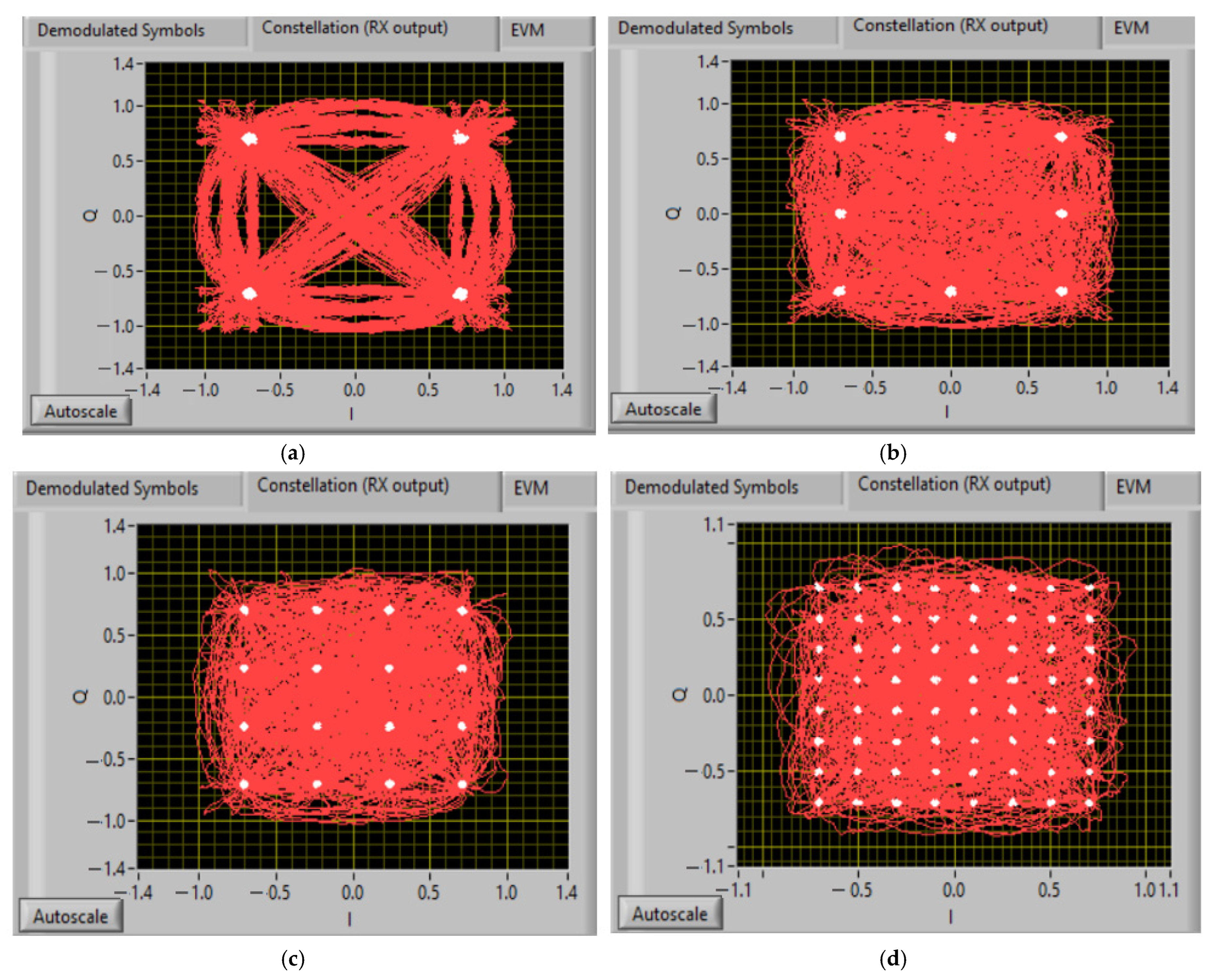
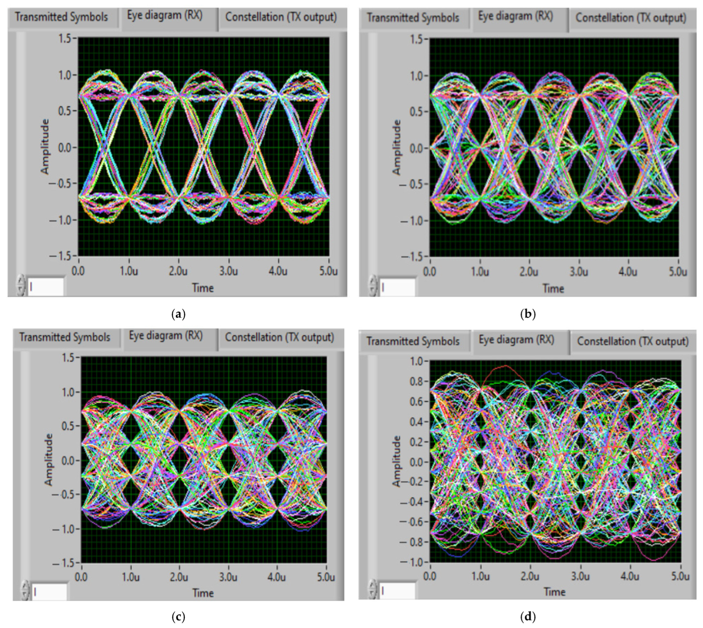
Quadrature amplitude modulation (QAM) is an increasingly used digital modulation scheme in modern telecommunications for transmitting information [7]. A QAM signal is a signal in which two carriers are phase-shifted by π/2 radians, and the resulting signal varies simultaneously in amplitude and phase. QAM transmits two signals by amplitude modulation for two carrier signals based on digital ASK (amplitude shift keying) modulation or the analog amplitude modulation (AM) scheme [8]. A variety of forms of M-QAM include 4/8/16/32/64/128/256/512/1024/2048/4096 QAM. Figure 1 shows the constellations of 4 QAM, 8 QAM, 16 QAM and 64 QAM communications, and Figure 2 shows the eye diagrams for the same types of modulations.

2.2. Jamming Attacks

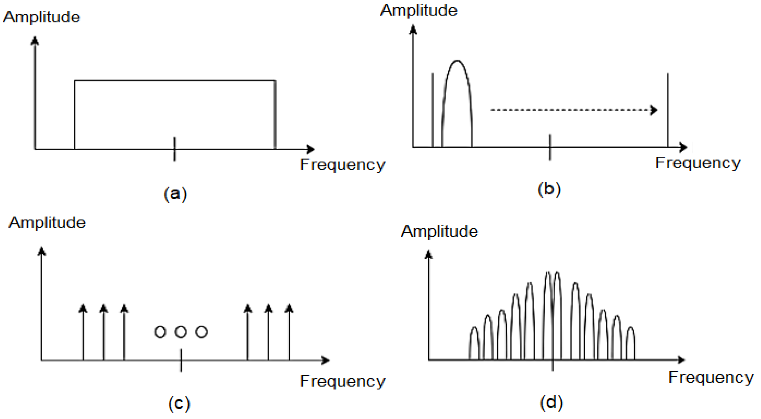
The most commonly used jamming types are barrage, sweep, protocol-aware, and tone. Figure 3 shows the frequency domain signals for the mentioned jamming methods. Barrage jamming amplifies a wideband noise signal [9]. The bandwidth of the noise signal could be as large as the bandwidth of a single channel, or it could be emitted over the entire frequency band of a communication. The advantage of barrage jamming is its low implementation complexity and its ability to jam any type of radio communication [10].
Also, because barrage jamming is effective for disrupting any type of radio communication, it also produces the most radio interference of all jamming types. Sweep jamming transmits a narrowband barrage signal in a “sweeping” motion over a full frequency band. The sweep speed is called the “sweep” speed. The advantages of this jamming device are that it can be implemented with little effort compared to the barrage jamming method [11]. If the “sweep” rate is high enough, the method can be combined with the barrage jamming method. Tone jamming divides the noise signal into discrete tones and can transmit the tones simultaneously (individually) or in a “sweep” motion that is used with a chirp jammer (chirp signal). The advantages of this type of jamming are the possibility of inducing less interference with other radio communications and its effectiveness for FHSS communications [12,13]. A protocol jammer (recognizes the protocol) imitates the original communication signal (as much as possible), using the same protocol but transmitting corrupted data [14]. The possibility of the receiver being more susceptible to picking up the jamming signal is pursued, starting from the idea that the receiver cannot filter the useful signal from the generated noise signal [15,16]. The disadvantage is that protocol jamming must be specifically tailored to a certain type of communication.
Even though additive white Gaussian noise (AWGN) represents the natural thermal noise of the universe, in EW this mathematical structure is used to create the most destructive type of intentional jamming: noise jamming. Within these EW attack methods, we distinguish the following types of attack:
1. Barrage Jamming (Barrage Jamming/Broadband Noise)
It represents the basic implementation of AWGN in EW. The attacker floods a very wide frequency band using exclusively Gaussian white noise generated at very high powers.
Purpose: To increase the noise floor so much that the receiver can no longer distinguish the useful signal (64-QAM in our case) from the noise.
Use: It is considered the most effective jamming when the attacker does not know the exact frequency or type of modulation used by the target.
2. Spot Noise Jamming (Directed Noise Jamming/Narrow Band)
Unlike the barrage, the attacker focuses all the AWGN energy on a single frequency of interest (or on a very narrow band).
Purpose: To concentrate the destructive power strictly on the frequency on which the 64-QAM signal is transmitted.
Use: To block fixed tactical radio channels or drone control channels.
3. Pulsed Noise Jamming (Pulsed Noise Jamming)
The attacker emits the AWGN signal in rapid bursts or short pulses, alternating periods of emission with periods of silence.
Purpose: To mislead the receiver’s adaptation algorithms and save the jamming station’s battery power.
Use: To test the robustness of forward error correction codes (FEC) and predictive algorithms (the Bi-LSTM network in the model proposed in the article).
Why does EW perform jamming using an AWGN signal? Motivation is determined by:
1. It is the most difficult to filter: Mathematically, Gaussian white noise contains all frequencies equally. A classic filter (notch filter) cannot eliminate it without damaging the useful 64-QAM signal.
2. Maximum blocking efficiency: Information theory (Shannon) demonstrates that the most harmful noise for the capacity of a communication channel is the one that follows the Gaussian distribution.

2.3. Wavelet Transform with SURE Soft-Threshold

In [17], Donoho and Johnstone propose another estimator based on soft-threshold truncation of wavelet coefficients, which considers both the input data and, therefore, both the signal and the noise, while adapting the threshold value as a function of the scale. Thus, for each level of the dyadic wavelet decomposition, a threshold value is determined based on Stein’s unshifted risk estimator (SURE). The computational effort is of the order of n log n . This estimator was named SURE Shrink. The application of the SURE in the case of soft-threshold truncation of wavelet coefficients can be performed as follows. For a vector v = v i : i = 1 d of dimension d, we consider observations x i N v i , 1 with a normal distribution with mean given by the vector v . Charles Stein introduced in 1981 a method for estimating the error v ^ v 2 in an unshifted manner [18].
Thus, v ^ = v x let be a particular estimator of v . Let v ^ x = x + g x , where g = g i i = 1 d is a function defined by R d R d . Then
E v v ^ x v 2 = d + E v g x 2 + 2 g x ,
where g = i x i g i .
Now consider the threshold soft truncation estimator v ^ i t = η S x i , and apply the Stein estimator. The quantity
S U R E t ; x = d 2 i = 1 d χ t , t x i + i = 1 d min x i , t 2
where χ t , t x i = 1 ,   for   x i t , t 0 ,   otherwise is an unbiased estimator of the risk function: E v v ^ t x v 2 = E v S U R E t , x .
Considering this risk function estimator, determine the threshold value for which the minimum is obtained,
t S = argmin t 0 S U R E t , x
The computational effort required to determine the threshold value t S is of the order of d log d .

2.4. Adaptive Channel Equalization Using Least Mean Square (LMS)

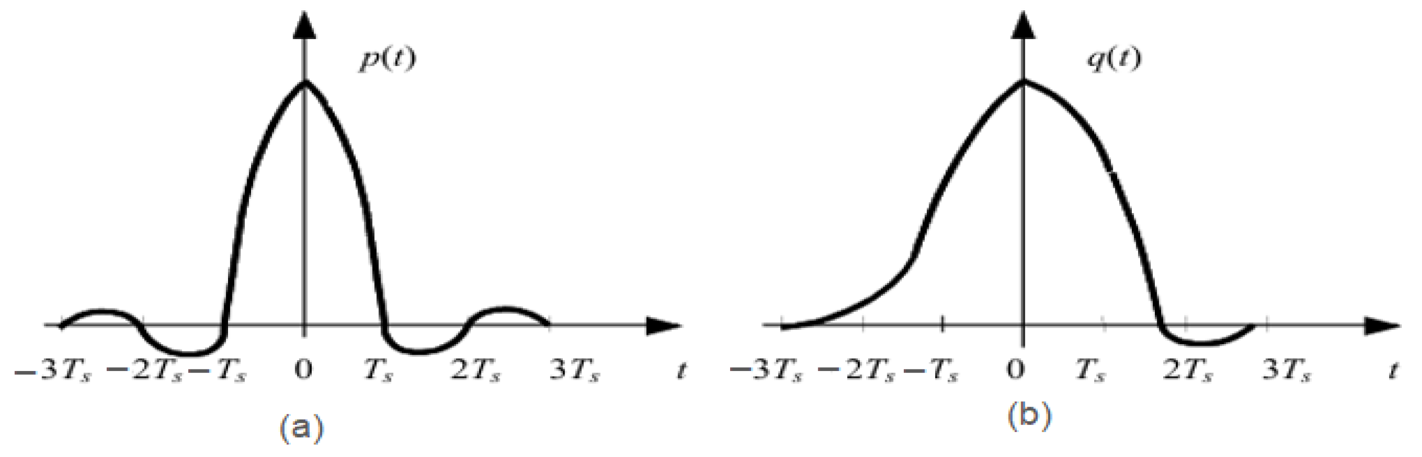
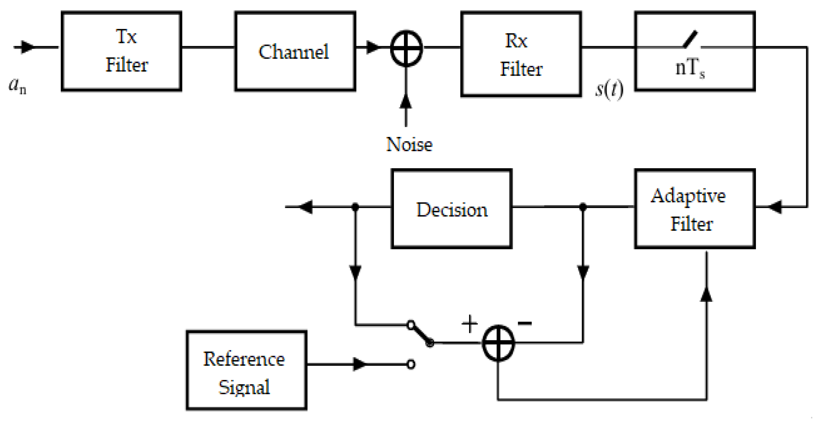
To illustrate the principle of adaptive channel equalization, consider a baseband data transmission system (Figure 4). In such a system, the data sequence a n is applied, at transmission, to a shaping filter, with the role of limiting the occupied bandwidth. A relatively wideband noise is introduced onto the communication channel [19].
At reception, to reduce this noise, a filter is used, and at the output the useful signal has the form [20]:
s t = k = 0 a k p t k T s  
T s represents the clock period, and p(t) represents the impulse response for the filter used for channel equalization.
In the case of a multi-level transmission, these can take the values ±1, ±3, …, ±2M−1; p(t) should ideally have a form like that in Figure 5a, so that:
p n T s = 1 ,   n = 0 0 ,   n 0
As a result, at any of the sampling times, of the form m T s , we have, disregarding noise,
s m T s = a m
So, the impulses do not influence each other.
The LMS algorithm has some similarities with the algorithm used in Wiener filter theory: it determines the optimal filter coefficients and is based on minimizing the squared error. Unlike Wiener filters, the LMS algorithm does not require the calculation of the correlation functions, rxx and rdx, but uses a recursive gradient method, known as the stepwise descent method, to determine the values of the filter coefficients that produce the minimum sum of the squared error [21]. In this method, the values of the filter coefficients are modified based on an estimate of the negative gradient of the error function with respect to a given set of coefficients:
b n k = b n 1 k + e n x ( n k )
where Δ—the quantity that characterizes (controls) the speed of the descending algorithm, known as the convergence rate of the LMS algorithm.
The choice of the value of this parameter requires some comments.
Thus, a large value of the convergence rate, Δ, leads to a substantial modification of the values of the filter coefficients, b n k , which will result in their faster convergence towards the set of optimal values, but can also lead to instability of the filter, manifested by the appearance of oscillations in its response.
Conversely, a too-small value of the convergence rate will lead to a slow convergence of the filter coefficients, with the consequence of a decrease in the speed of the receiver’s reaction to the input signals and a decrease in its probability of interception.
The use of adaptive filtering as a signal processing step in equalizing a communications channel subjected to electronic warfare jamming, to eliminate the noise component, can take two distinct forms:
Removing narrowband noise from a wideband signal (also known as adaptive interference suppression);
Removing wideband noise from a narrowband signal (also known as adaptive noise suppression).
Since wideband noise suppression is much more common in practice, the paper addresses the modeling of LMS adaptive filtering for this situation.

2.5. Bidirectional Long Short-Term Memory (Bi-LSTM)

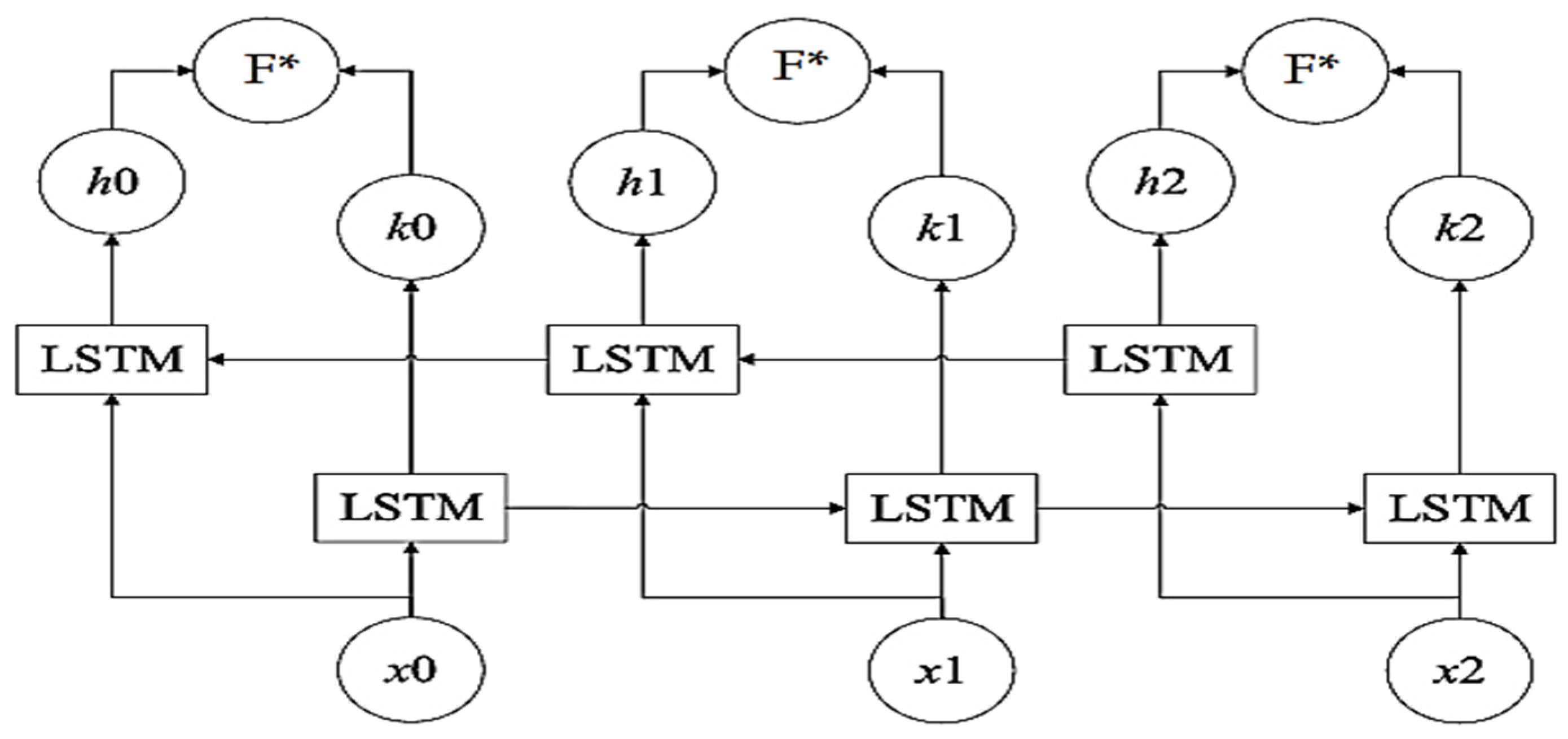
The Bi-LSTM structure consists of a forward LSTM module and a backward LSTM module. The LSTM architecture for each layer determines and generates the information vectors for the hidden state, and the parameterization information of the model is updated and determined by backpropagation. Using the gate functions, these determine the strategy for sequentially changing the time intervals and the delays determined by the evolution of the time-varying (temporal) series [22,23].
LSTM models time series data by vectorizing state parameters h and c, which describe the data model being studied. An LSTM memory layer is described by Formulas (1)–(6).
f t = σ W f x t + U f h t 1 + b f ,
i t = σ W i x t + U i h t 1 + b i ,
o t = σ W o x t + U o h t 1 + b o ,
c ~ t = t a n h W c x t + U c h t 1 + b c ,
c t = f t ° c t 1 + i t ° c ~ t ,
h t = o t ° t a n h c t ,
where σ represents the activation sigmoid function and tanh represents the hyperbolic tangent applied to each element of the state vector. The operator (°) represents the Hadamard distance that is used for each component, f t represent the forgetting threshold layer, o t is the output threshold layer, and W f , b f , W i , b i , W o , b o are the weights and offsets of each threshold layer, respectively [24].
The Bi-LSTM architecture is illustrated in Figure 6, where the parameters x0, x1 and x2 are the input parameters for the time sequences 0, 1 and 2; h(0–2) and k(0–2) represent the output vectors of the hidden salts for a certain time instant; and the F* function represents the concatenation vectors [25].
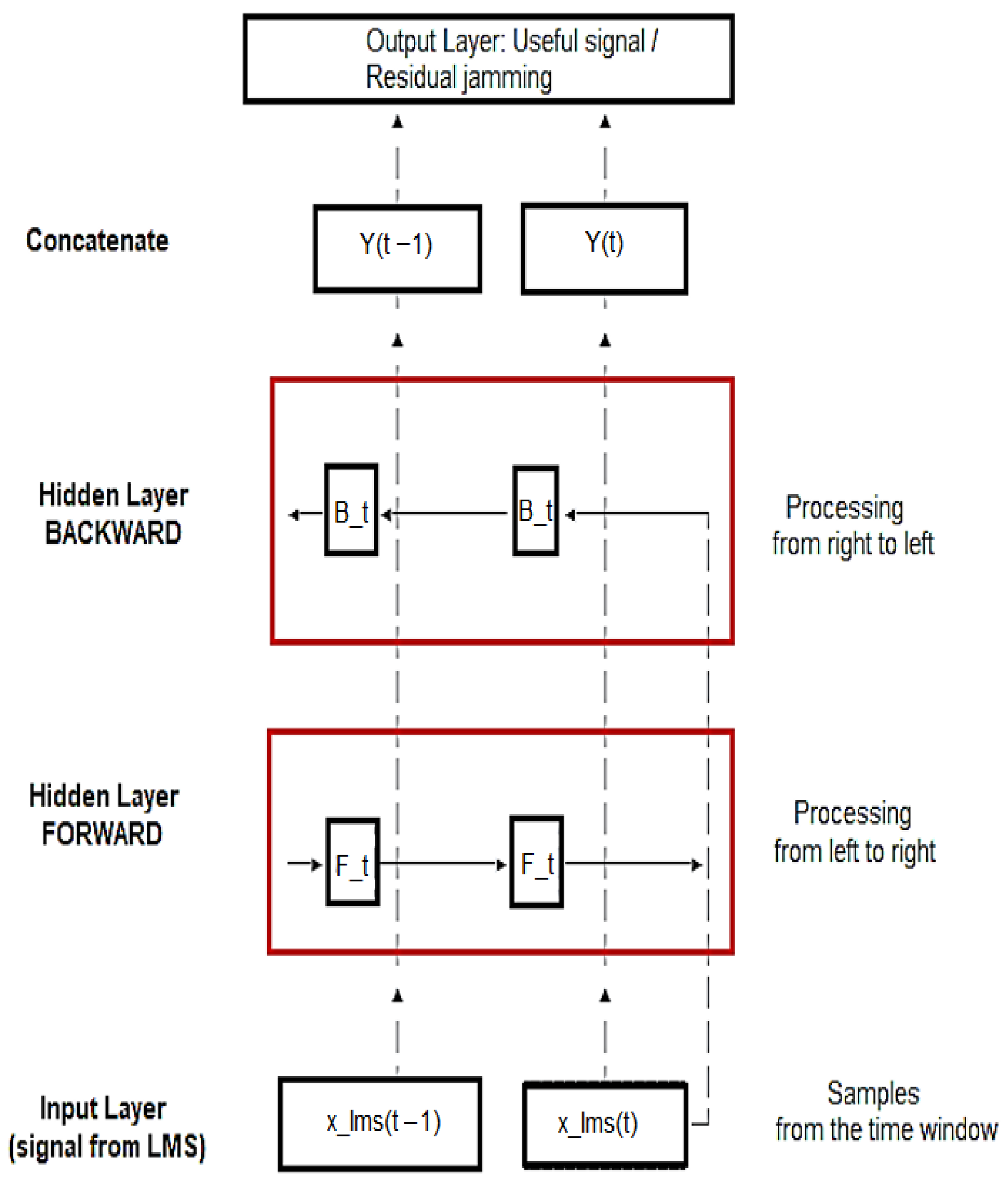
Since LMS filtering introduces phase and inter-symbol (ISI) distortions into the 64-QAM constellation, in the final processing stage we use the Bi-LSTM network. The advantage of the bidirectional architecture lies in the ability to process the symbol sequence both in the forward direction (past context) and in the reverse direction (future context). An LSTM cell processes the input vector composed of the real and imaginary parts of the signal (I/Q): x t = R y n , J y n . The equations of the layers (attenuation, input, output) are defined as:
i t = σ W i x t + U i h t 1 + b i
f t = σ W f x t + U f h t 1 + b f
o t = σ W o x t + U o h t 1 + b o
The cell state c t  and the hidden output h t combine the forward ( h t ) and backward ( h t ) flows:
h t b i = h t h t
h t = L S T M f w d x l m s , t , h t 1 , h t = L S T M b w d x l m s , t , h t + 1 ,  
The final Dense (Fully Connected) layer maps the h t b i vector directly into the correct coordinates of the 64-QAM I/Q space.
The diagram of the bidirectional LSTM (Bi-LSTM) architecture is shown in Figure 7.
Optimization Algorithm: Adam (Adaptive Moment Estimation)
The updating of the θ parameters is performed by the Adam (Adaptive Moment Estimation) algorithm, which combines the advantages of the RMSProp (Root Mean Square Propagation) and Momentum algorithms. It calculates adaptive learning rates for each parameter based on the estimates of the first moment (mean) and the second moment (uncentered variance) of the gradients:
m t = β 1 m t 1 + 1 β 1 g t
v t = β 2 v t 1 + 1 β 2 g t 2
where g t = θ L θ t = L W t is the gradient of the loss function at step t, and β 1 , β 2 [ 0 , 1 ) are the hyperparameter coefficients for the exponential decomposition. After bias correction:
m ^ t = m t 1 β 1 t , v ^ t = v t 1 β 2 t
The final parameter update rule becomes:
θ t + 1 = θ t η v ^ t + ε m ^ t ,     W t = W t 1 η v ^ t + ε m ^ t
where η is the fixed learning rate ( η = 10 4 ), and ε is a numerical stability constant ( 10 8 ) used to prevent division by zero.
Where the standard hyperparameters used are η = 0.001 (learning rate), β 1 = 0.9 ,   β 2 = 0.999 and ε = 10 8 .
For the validation of the method, the parameters and simulation configuration for the proposed model are presented in Table 1.
Architecture and Hyperparameters of the Bi-LSTM Network
The network is designed to map distorted sequences directly into linear I/Q coordinates. Table 2 shows the hyperparameter configuration.
Loss Function
The loss function used for network optimization is the mean square error (MSE), calculated on the data batch (batch) as the Euclidean distance in the complex plane:
L M S E = 1 B · L b = 1 B t = 1 L I b , t I ^ b , t 2 + Q b , t Q ^ b , t 2
where
B is the batch size (batch size = 256).
L is the sequence length (L = 64).
I b , t and Q b , t are the actual coordinates transmitted at time t for sample b.
I ^ b , t and Q ^ b , t are the predicted values at the output of the Bi-LSTM network.
Overfitting Prevention Strategy
In addition to Early Stopping, a Dropout layer of 0.2 was introduced between the two Bi-LSTM layers to randomly deactivate 20% of the connections during training. This forces the network to learn generalized geometric features of the constellation, preventing it from simply memorizing specific noise sequences or transient phases of the LMS filter.

3. Results

3.1. Proposed Architecture for Restoring 64 QAM Affected by Jamming

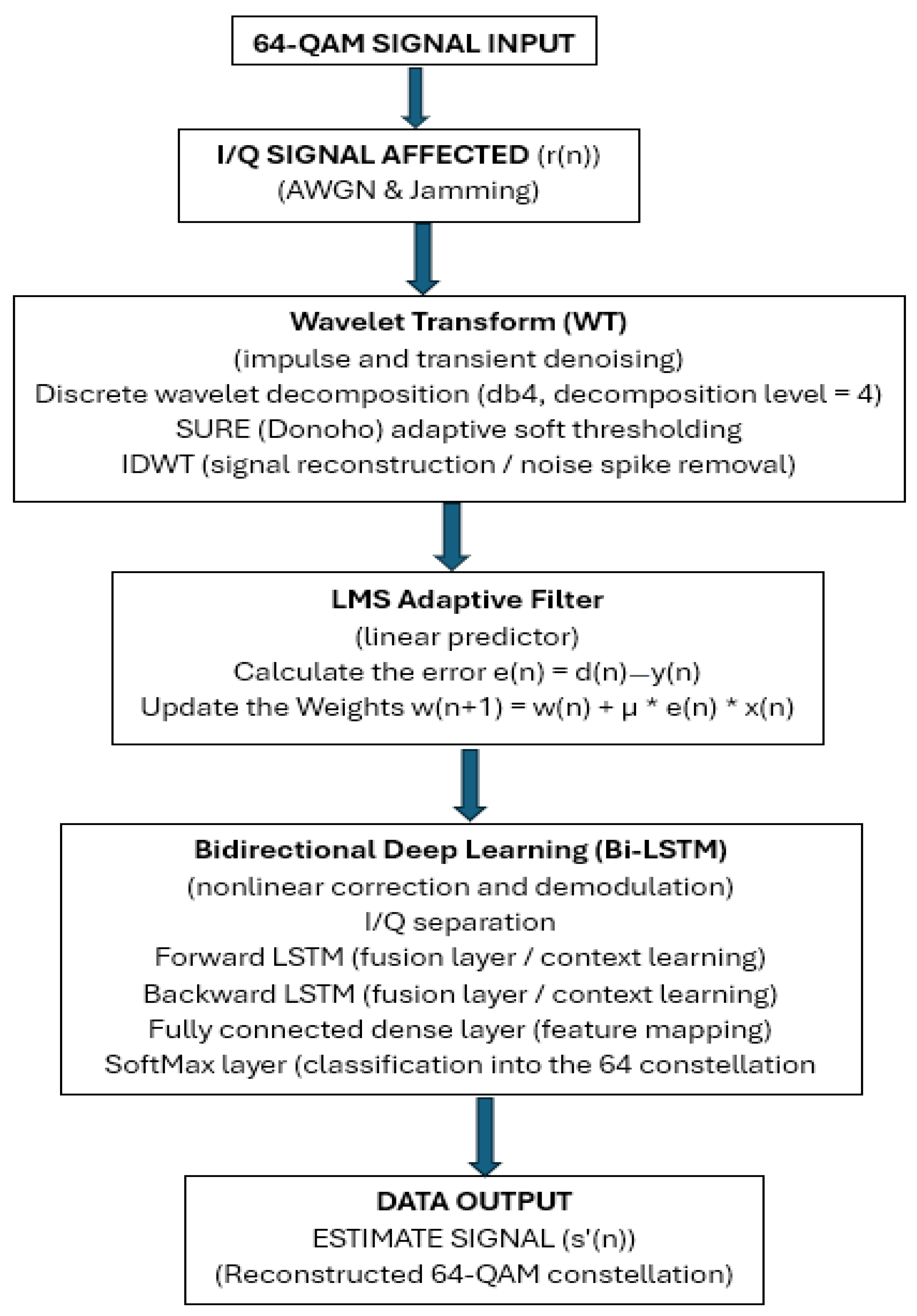
Figure 8 shows the model proposed in the article. The computational architecture goes through the following stages: acquisition of historical data used for training the system and in real time for validation, data preprocessing using SURE thresholder wavelet transform for denoising and vectorization, identification and extraction of specific features for communication channel analysis, optimization of mechanisms of channel equalization using LMS for determining decision parameters and prediction using equalization schemes based on LMS-Bi-LSTM.
Explanation of the Data Flow in the Diagram shown in Figure 8:
Input Module: The signal (r(n)) combines the useful 64-QAM bits with the natural AWGN background noise and the external electromagnetic attack (barrage jamming with AWGN).
Operation of Stage 1 (WT): Decomposes the signal into frequency sub-bands. Impulsive (short and high power) jamming components appear as extreme values in the detail coefficients and are instantly “cut off” by the thresholding algorithm before signal reconstruction by IDWT.
Operation of Stage 2 (LMS): The impulse-cleaned signal enters the adaptive filter. LMS dynamically adjusts the coefficients to estimate and cancel by subtraction continuous jamming signals (such as sinusoidal jamming tones or fixed carriers).
Stage 3 Bi-LSTM Operation: The points in the constellation are still distorted by channel fading and residual noise. The neural network analyses the transmitted symbols both forward and backward. It corrects for phase and amplitude distortions, placing each symbol with maximum precision in the correct 64-point mapping of the constellation.
The results obtained when testing the proposed LMS-Bi-LSTM model for achieving channel equalization and recovering and restoring 64 QAM from the AWGN generated by the jamming system are presented in the following subchapter.

3.2. Training Methodology and Experimental Setup

Signal and Dataset Generation Procedure
The dataset was synthetically generated in a controlled environment to accurately model a communications channel disturbed by noise. The generation procedure is:
Useful Symbol Generation: A sequence of pseudo-random bits is generated, grouped in blocks of 6 bits, mapped according to a standard 64-QAM constellation with energy normalization ( E s = 1 ).
Channel Modeling and Interference Introduction: Additive white Gaussian noise (AWGN) is added over the useful signal s[n] to cover a range E b / N o 0 , 25 dB.
Jamming: Randomly add Single-Tone (STJ) and Partial Bandwidth (PBJ) jamming, with a signal-to-noise ratio (JSR) dynamically varying between −15 dB and +10 dB, with a step of 2 dB.
Preprocessing (wavelet + LMS): The raw distorted signal r[n] is passed through the wavelet noise reduction block (SURE thresholding) and then through the LMS adaptive filter.
Data Pair Formation (Features and Targets):
Network Input (X): The tensor of dimensions [N × L × 2], representing the In-phase (I) and Quadrature (Q) components of the signal after LMS filtering.
Network Target (Y): The ideal I/Q coordinates of the initially transmitted 64-QAM symbols.
Data Size and Splitting
Total Data Volume: A total of 1,200,000 64-QAM symbols were generated.
Sequence Length (L): The signal was segmented into sliding windows of length L = 64 symbols, ensuring an optimal balance between network memory and computational complexity. The windows use an overlap of 50%.
Dataset Splitting:
Training Set: 70% (840,000 symbols), used for weight adjustment.
Validation Set: 15% (180,000 symbols), used for monitoring overfitting and applying Early Stopping.
Testing Set: 15% (180,000 symbols), kept completely isolated for the final BER evaluation.

3.3. Testing Stage

This subchapter presents the results obtained from the evaluation tests of the WT-LMS-Bi-LSTM model for equalizing the 64 QAM communication channel disturbed by jamming systems. For the tests, we used the 64 QAM communication parameters of the drone specified for the remote control (RC) of the drone. Table 3 presents the technical parameters for the RC link for the Microhard model pMDLL 1624-AES 256 (source: https://www.microhardcorp.com/brochures/pMDDL1624.Brochure.Rev.1.0.8.pdf, accessed 13 March 2026).
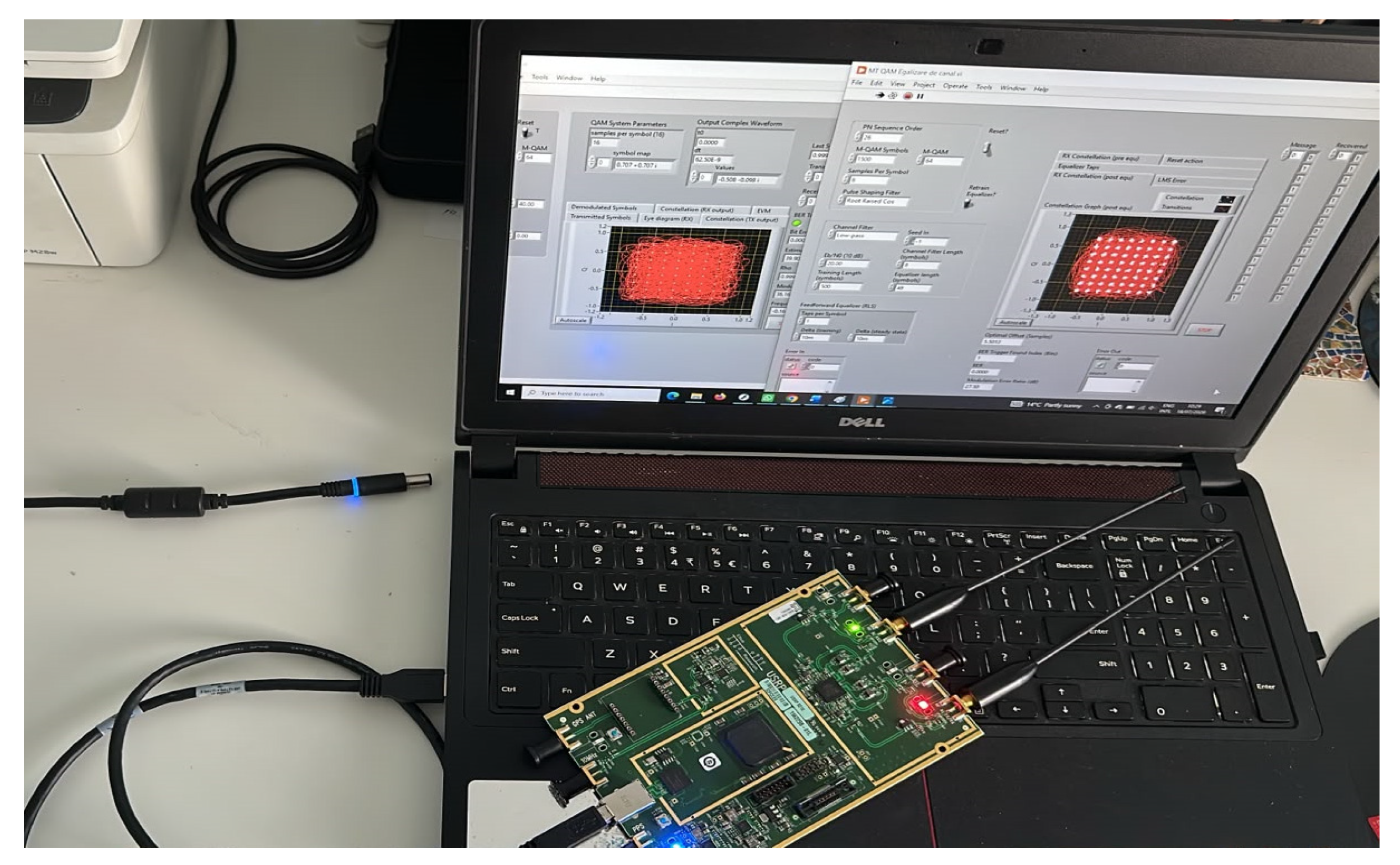
To carry out the laboratory tests, we implemented the RC communication of the drone (Tx/Rx) on a USRP Ettus B210 (manufacturer: Ettus Research, Austin, Texas, USA; source: https://files.ettus.com/manual/page_usrp_b200.html, accessed 12 January 2026) software-defined radio (SDR). The Tx (USRP red LED) and Rx (USRP green LED) software applications were developed in the LabVIEW programming language (version 2022 Q3; manufacturer: National Instruments, USA). The laboratory model implemented for the tests is presented in Figure 9.
The test architecture is shown in Figure 9.
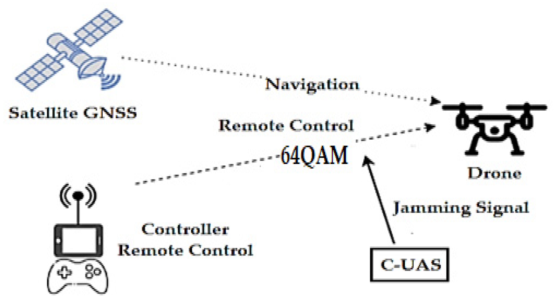
According to Figure 9, the RC signal with 64 QAM is affected by a Gaussian white noise jamming signal, which is the most used jamming signal (C-UAS).
For the laboratory simulation using the USRP Ettus B210, instead of drone communication, the following parameters were used: frequency 1.625 MHz, bandwidth 1 MHz, PN sequence order 26, QAM symbols 1500, samples per symbol 6, symbol rate 1 M, transmitter–receiver distance according to Figure 10, AWGN and Rayleigh channel model, variable SJR −15 dB/+10 dB, sampling rate 61.44 MS/s (USRP Ettus B210).
The results obtained during the tests are presented below.
Step 1—64 QAM signal reception
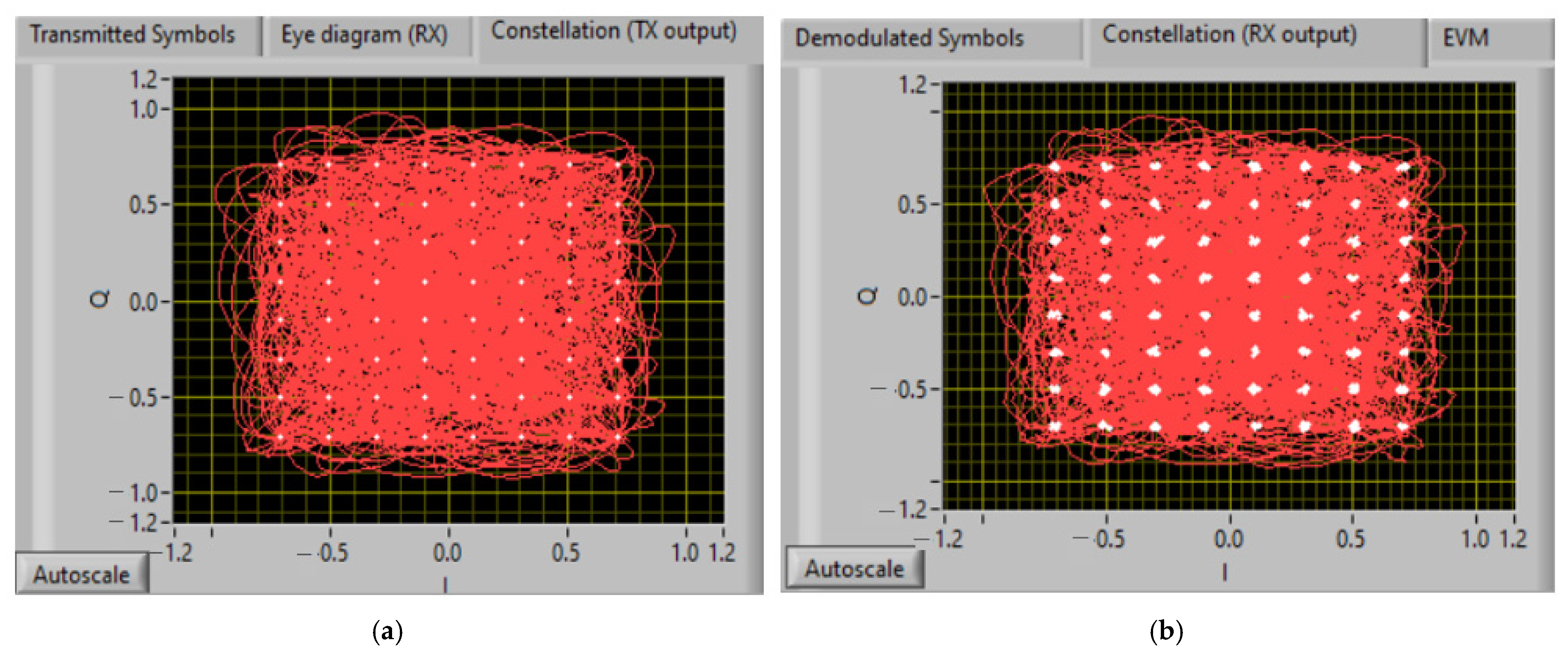
Figure 11 shows the 64 QAM constellations for transmission (TX) and reception (Rx).
To evaluate the jamming noise signal (interference) tolerance for digital modulations, the following indicators are used: BER (bit error rate), energy per bit-to-noise power spectral density ratio (Eb/No), MER (modulation error ratio) and constellation diagram.
MER—modulation error ratio (MER) is a measure of the signal-to-noise ratio (SNR) in a digitally modulated signal. MER is usually expressed in dB.
BER—bit error rate (BER) is defined as a measure of the number of bit errors occurring in a specified number of bit transmissions, typically expressed as a ratio.
Eb/No represents the signal-to-noise ratio for a digital communication.
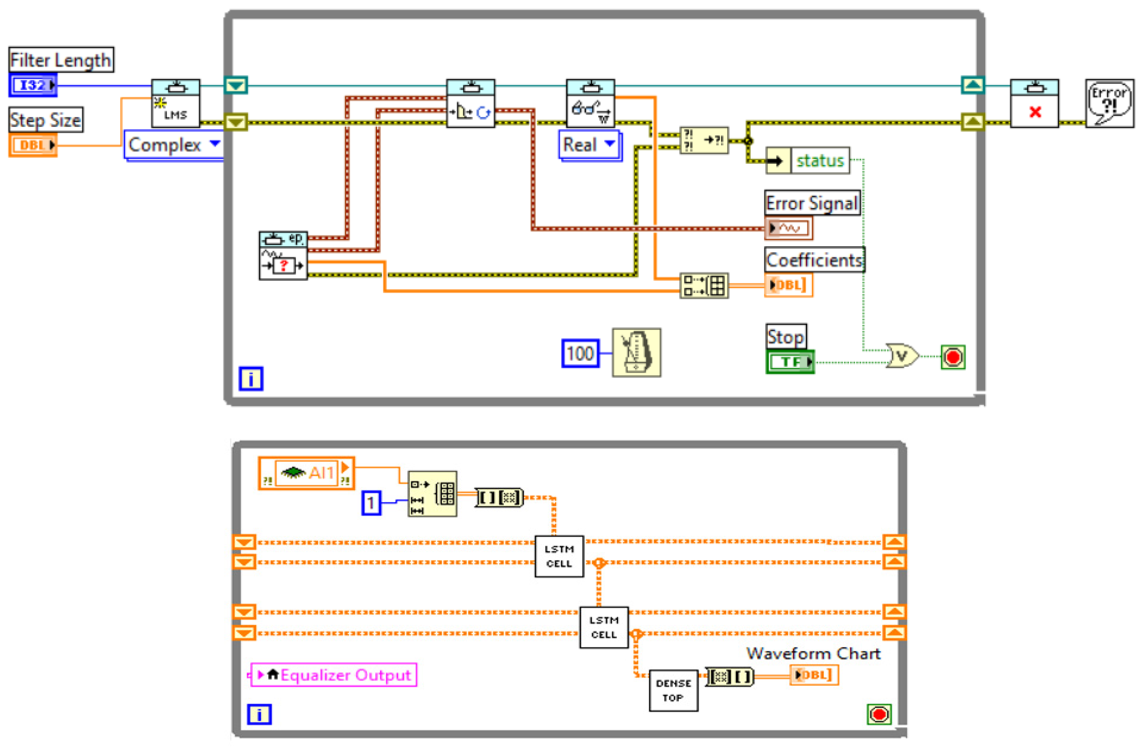
Figure 12 shows the software implementation of the proposed LMS-Bi-LSTM algorithm for channel equalization perform in LabVIEW.
Step 2—Training the LMS-Bi-LSTM model
Within the adaptive filter (LMS algorithm), statistical calculations are replaced with the weighted sum of squares of the temporal values, an aspect that gives this filter increased performance characteristics and design robustness. Thus, the cost function, instead of the MSE, is replaced by the least squares (LS) cost function.
Comparison of LMS with RLS:
  • Convergence in RLS is approximately an order of magnitude faster than in LMS;
  • Unlike LMS, convergence in RLS does not depend on the spread of the input signal eigenvalues;
  • RLS is superior due to its convergence and adaptation power;
  • The computational effort in RLS is high compared to LMS;
  • RLS can achieve a trade-off between computational complexity and performance of adaptive filtering.
Considering the above, in this paper we opted for modeling and using the LMS algorithm to improve the signal-to-noise ratio in the preliminary processing of signals from the drone receiver affected by the jamming generated by electronic warfare equipment.
To successfully train and evaluate a Bi-LSTM neural network combined with WT and LMS for 64-QAM, the training dataset must cover a wide range of channel conditions. To ensure the convergence of the network and its generalization (ability to recognize sweep and multitone jamming at various intensities), specific values are used for the parameters E b / N o , MER and BER.
1. The parameter E b / N o (energy per bit relative to noise spectral density)
E b / N o is the main parameter used to control the background noise (AWGN) in the generation of the dataset. For 64-QAM, the range of values used for training is strategically divided into different values shown below:
  • Training Range: between 0 dB and 25 dB (in 1 dB or 2 dB steps). Below 8 dB, the noise is so destructive that the 64-QAM constellation completely loses its geometric structure, and the network learns only pure noise (risk of underfitting). Above 22–25 dB, the channel becomes almost ideal, and the jamming is extremely easy to detect. Training in the critical transition zone (10–18 dB) forces the Bi-LSTM network to learn exactly the boundaries of the 64-QAM decision regions
2. MER (modulation error ratio) parameter
MER measures the total vector distortion of the constellation (the cumulative effect of noise, sweep and multitone jamming). In the training dataset, the MER values at the network input serve as attack severity indicators.
Bi-LSTM input values (heavily noisy channel): between 10 dB and 22 dB. A MER below 23 dB for 64-QAM means a completely degraded constellation (“clouds” of overlapping points), where classical decoding fails. The network is trained intensively on these low-MER samples to learn the dynamic jamming trajectory
Target output values (after cleaning): ≥27 dB–30 dB. This is the optimization goal of Bi-LSTM. Once the jamming is removed, the MER should return above the industrial safety threshold (23 dB + margin)
3. BER (Bit Error Rate) parameter
BER is not directly introduced as a feature in the input I/Q matrix but is the control parameter of the labels (labels/ground truth) and the performance metric of the loss function (loss function).
Pre-FEC BER (input): between 0.05 (5 × 10⁻²) and 0.15 (1.5 × 10⁻¹). This is the level of error induced by the combined raw sweep and multitone noise (such as the 0.063 value discussed earlier). The dataset contains these massive errors so that the model can understand the deviation of the I/Q vectors.
Post-Bi-LSTM BER (training target): ≤10−3 (0.001). The loss function (usually Mean Squared Error—MSE) penalizes the network until the reconstructed I/Q vectors reach a geometric accuracy that guarantees a BER below 10−3, allowing subsequent decoders to function correctly. Table 4 presents the parameters used to train the system using dataset setup (scan interval) and training parameters (critical values and success value). If you want to define the “Dataset Setup and Training Parameters”, we can use exactly this standard mathematical structure:
Step 3—Performing Rx 64 QAM jamming using AWGN
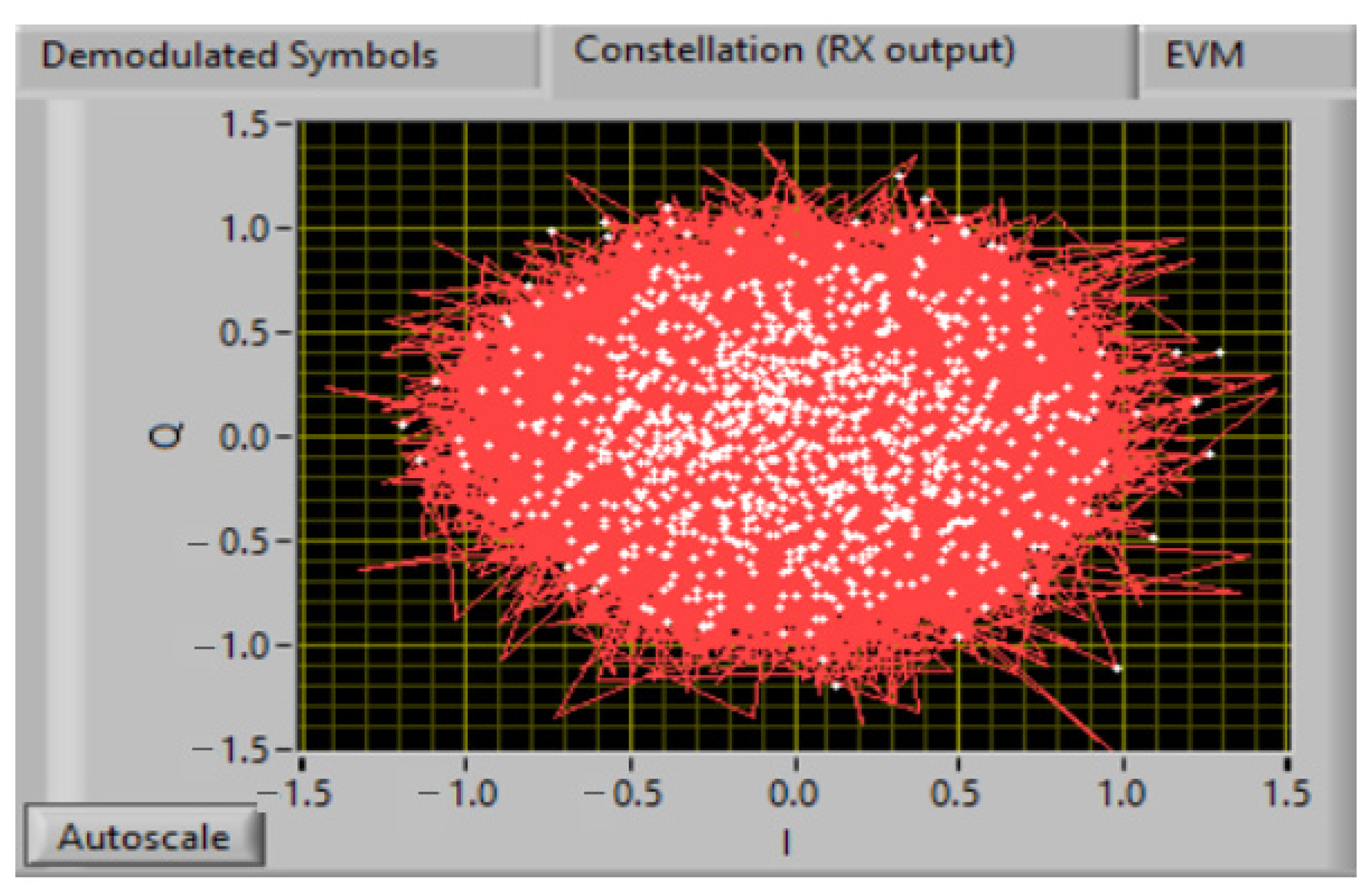
Figure 13 shows the reception of the 64 QAM constellation communications to the Gaussian white noise jamming attack.
Step 4—Denoising 64 QAM using SURE thresholder wavelet transform
The algorithm proposed by Donoho for the purpose of reconstructing a signal f t i = f i from its degraded samples of additive Gaussian white noise, y i = f i + σ z i , z i N 0 , 1 being the normalized samples of the noise, is practically implementable as it consists of three stages.
The three stages of the algorithm are:
1. Applying a pyramidal wavelet transform on the input data, thus obtaining a set of wavelet coefficients w i i = 1 n .
2. Processing the wavelet coefficients through a nonlinear threshold truncation operation, of the form
w ^ i = sgn w i w i t h + , i = 1 , n
where
x + = x , for   x > 0 0 ,   otherwise
and t h is a threshold value, called the universal threshold, which is calculated by the formula t h = σ 2 log n , σ being the noise dispersion and n the number of samples.
This nonlinear operation is called soft-thresholding by the author.
3. On the coefficients modified by the threshold truncation operation,
The inverse transformation is applied, thus obtaining the estimate of the original signal, f ^ i .
As can be seen, coefficients with absolute values lower than the threshold value are reduced to zero, this being motivated by the fact that most such coefficients are determined by noise.
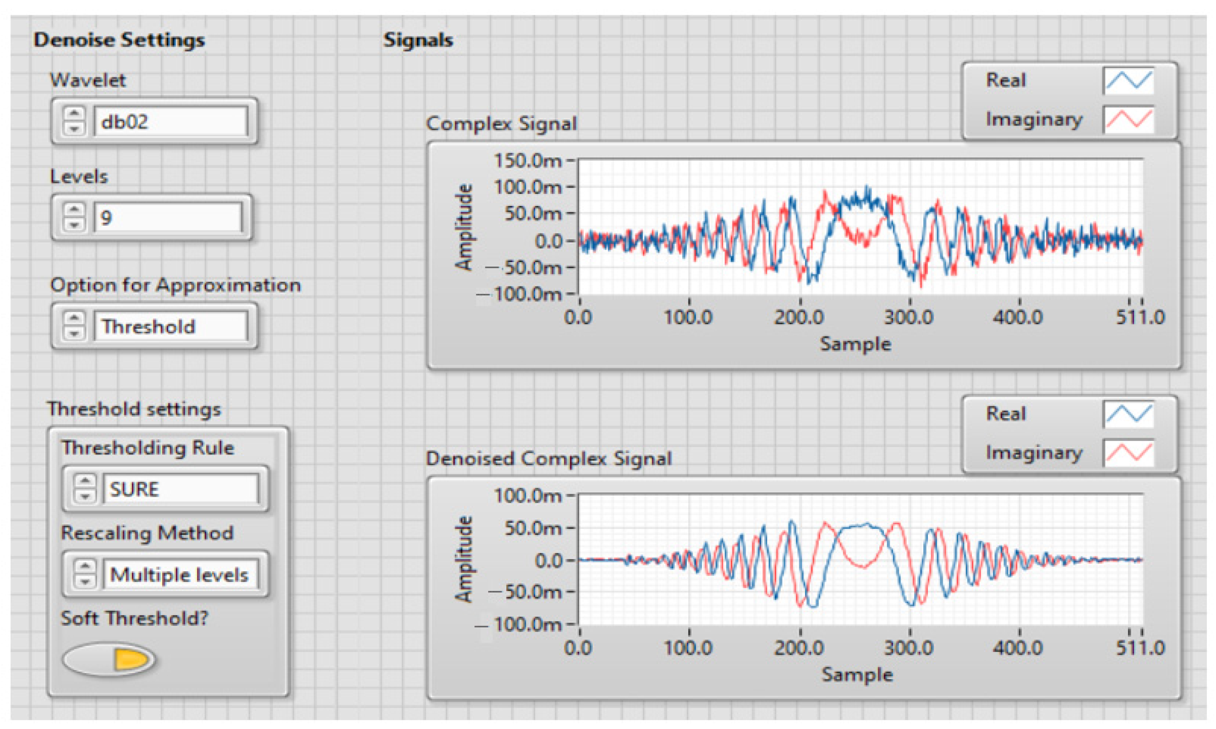
The reconstruction of the signal by the proposed procedure has two useful properties. The first is that in the reconstructed signal, with a very high probability, the noise is no longer present; only very few random oscillations are observable, some of which are associated with noise. The second property consists of the fact that if the original signal presents abrupt variations, then these are found, almost identically, in the reconstructed signal. Figure 14 shows the result obtained for noise reduction from the complex IQ signal related to 64-QAM modulation using WT, Daubechies 2 (db02), decomposition level 9 and the SURE soft threshold.
The method of noise reduction by soft-thresholding wavelet coefficients has been successfully used in many applications, such as medical signals and images, signals from geophysical measurements or from synthetic aperture radars, and even for removing artifacts generated by low-bitrate image compression.
Although the method of noise reduction by soft-thresholding of wavelet coefficients yields estimates at least as smooth as the original function and no spurious oscillations are present in the estimated solution, there is a trade-off between noise suppression and over-smoothing of details in complex radio communication signals.
Step 5—Testing channel equalization with the proposed LMS-Bi-LSTM model
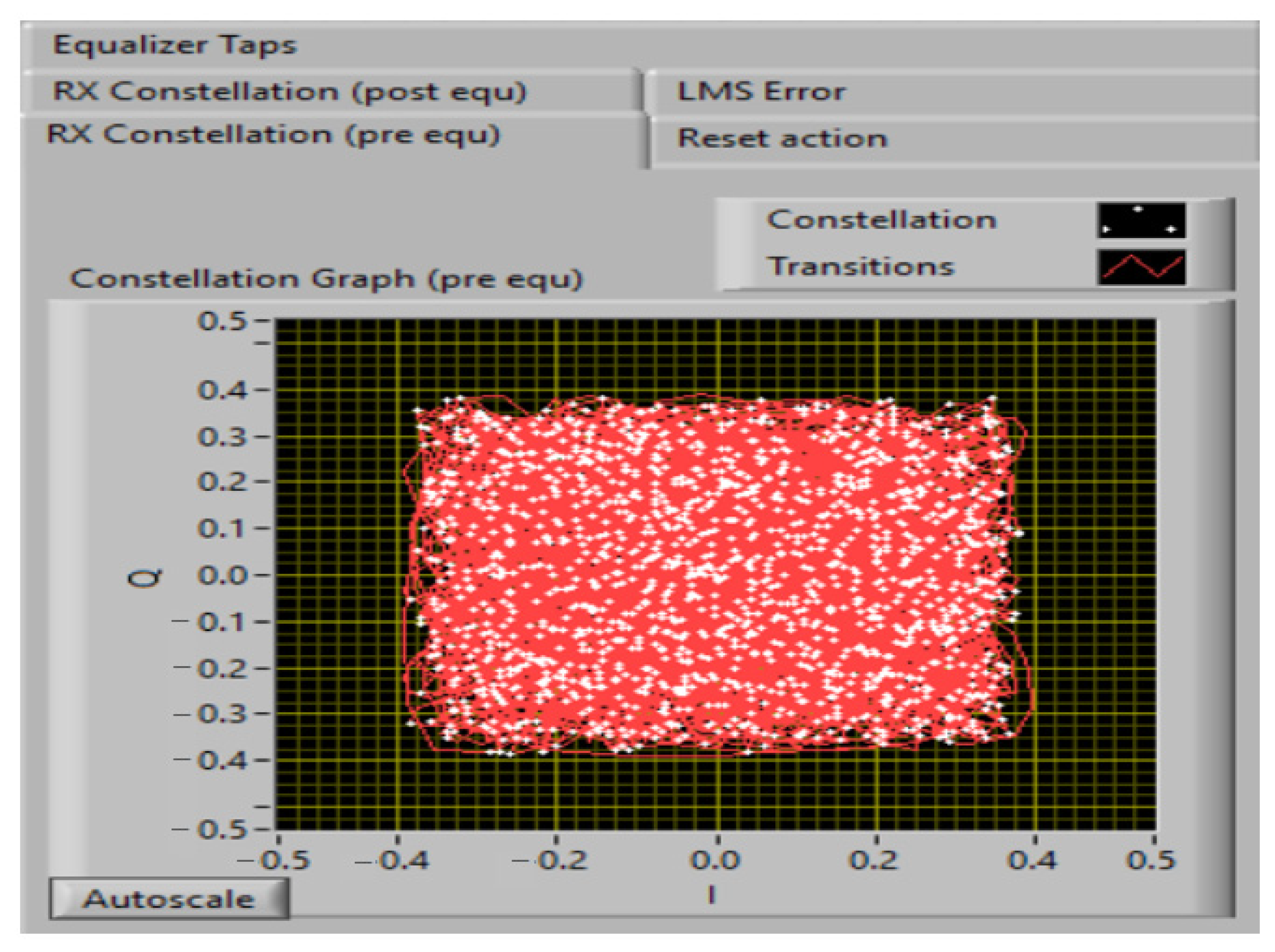
Figure 15 shows the 64 QAM constellation affected by jamming in the pre-equalization stage with the reception parameters BER = 0.087, MER = 6.16 dB, Eb/No = 10.50 dB.
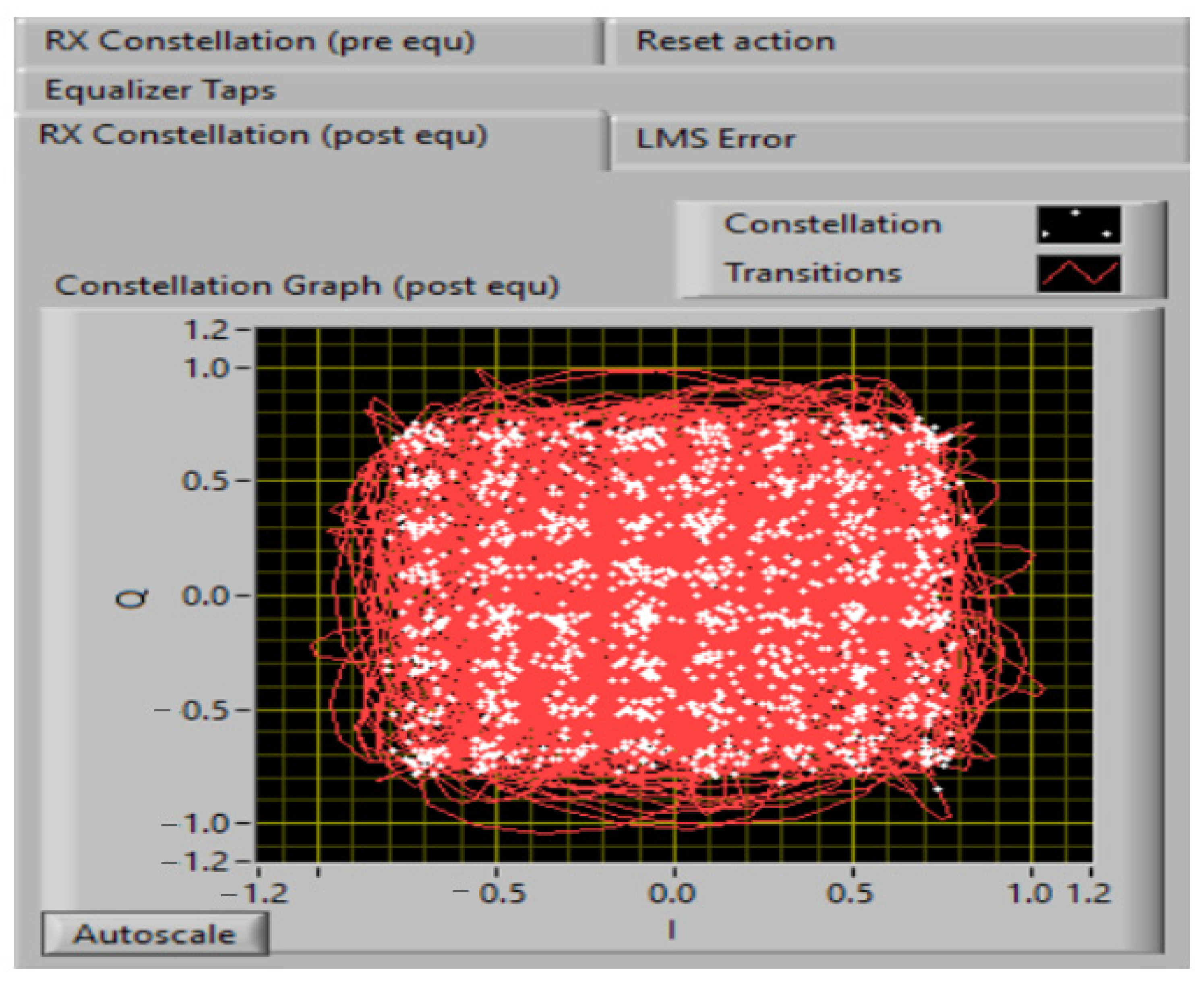
Figure 16 shows the 64 QAM constellation affected by jamming in the post-equalization stage with the reception parameters BER = 2.0 × 10 3 , MER = 27.44 dB, Eb/No = 20.50 dB.
Configuring the Matrix Structure of I/Q Data at the Input of the Bi-LSTM Network
Since LSTM deep learning networks cannot natively process complex numbers ( I + j Q ), the signal received after the WT and LMS stages must be decomposed and mapped into a multidimensional tensor structure (matrix) adapted to temporal processing.
Extraction of Real and Imaginary Components
The complex signal at the output of the LMS, for a block of length N, is defined as:
x l m s n = I n + j · Q n ,           n = 1,2 ,   . ,   N
Each sample is separated into two real features: I n , Q ( n ) .
Sliding Window Technique
To allow the Bi-LSTM network to learn the temporal dynamics and correlations between samples (both past and future), the data is structured using a fixed-length sliding window T (e.g., T = 50 samples) and a step of movement S = 1.
Input Tensor Structure (Shape)
The standard format required by the input layers of recurrent networks is a 3D tensor of the shape:
X i n R B × T × F
where:
B (Batch Size): The number of time windows analyzed simultaneously during a training or inference iteration (e.g., 32, 64 or 128).
T (Time Steps/Window Length): The size of the time window (sequence length). Determines the direct contextual memory of Bi-LSTM (e.g., 50).
F (Features): Number of features per sample. In our case, F = 2 (component I and component Q).
Input Matrix for a Single Batch:
For a single window in the batch, the data matrix M R T × 2 passed to Bi-LSTM has the following internal configuration:
M = I t T + 1 Q ( t T + 1 ) I t T + 2 I ( t 1 ) Q t T + 2 Q ( t 1 ) I ( t ) Q ( t ) T × 2
Output Tensor Structure (Target)
The network is trained in supervised mode (Supervised Learning). The goal of the final Dense layer after Bi-LSTM concatenation is to predict only the residual nonlinear jamming components J ^ I t , J ^ Q ( t ) for the current sample. Therefore, the target vector (ground truth) for each window has the size {1 × 2].
The proposed LMS-Bi-LSTM channel equalization algorithm model was trained and verified separately for different values of Eb/No.
Bi-LSTM network testing procedure, evaluation protocols and metrics used for performance validation
Performance Evaluation and Testing Protocol
The testing of the proposed hybrid network was performed on the completely isolated test set (containing 180,000 64-QAM symbols), not used in the training or validation phases. The purpose of this protocol is to evaluate the generalization capacity of the model under extreme conditions of noise and variations in the signal-to-noise ratio.
Test Running Protocol
The testing process follows a strict three-step flow on streaming data:
Segmentation: The received signal is pre-filtered by the WT-SURE and LMS blocks and divided into windows of length L = 64, with no overlap, to achieve a real-time reception scenario.
Inference (Forward Pass): The test tensor X t e s t of size [M × 64 × 2] is passed through the trained Bi-LSTM network to generate the predictions of coordinates I ^ and Q ^ .
Decision and Demodulation: The continuous coordinates estimated by the network are passed to a Hard-Decision (Nearest Neighbor Demodulator) decision block, which maps each estimated point to the nearest ideal symbol in the standard 64-QAM constellation.
Performance Metrics Evaluated
For exhaustive validation, network performance is not measured only by the loss function (MSE), using metrics specific to digital communications:
A. Bit Error Rate (BER)
It is the fundamental metric of the system. It measures the ratio between incorrectly decoded bits and the total number of transmitted bits:
B E R = N u m a r   b i t i   e r o n a t i N u m a r   t o t a l   b i t i   t r a n s m i t i
Since each 64-QAM symbol carries l o g 2 64 = 6   b i t i , the symbol error is converted into bit error by directly comparing the bit diagrams (Gray mapping).
B. Error Vector Magnitude (EVM)
EVM measures the geometric distance between the recovered symbol and the ideal one in the complex I/Q plane, being a direct indicator of the signal quality before the hard decision:
E V M % = 1 N n = 1 N y i d e a l n y e s t i m a t n 2 P a v g × 100
where P a v g is the average power of the standard 64-QAM constellation, and y n = I n + j Q [ n ] .

3.4. Implemented Testing Scenarios

The network was subjected to two stress tests to highlight the superiority of the proposed solution over the classical solutions:
Test 1: SJR (Signal-to-Jamming Ratio) Variation: The E b / N o ratio was kept fixed at 20 dB (low background noise), while the jamming power was increased quite a lot, varying the SJR from +10 dB to −15 dB.
Test 2: Tracking Dynamics (Jamming Frequency Switch): An attack was simulated in which the Single-Tone jamming suddenly changes its frequency in the middle of the test time, evaluating the ability of the Bi-LSTM network to instantly compensate for the re-convergence period (transient error) of the LMS filter.
After running the tests, the following average values were obtained on the independent dataset (Table 5).
Analysis of Testing Behavior:
  • Resistance to phase rotations: The EVM test demonstrates that while the LMS filter leaves a residual phase error due to stochastic adaptation (EVM of 22.1% at −10 dB), the Bi-LSTM network reduces this error to only 5.4%. The constellation points become perfectly compact.
  • Temporal prediction ability: In the frequency hopping noise scenario, the temporal analysis of the BER showed that the proposed system does not exhibit error bursts. The backward layer of the Bi-LSTM uses the future symbols (already stable) to correct the past symbols affected by the LMS phase transition.
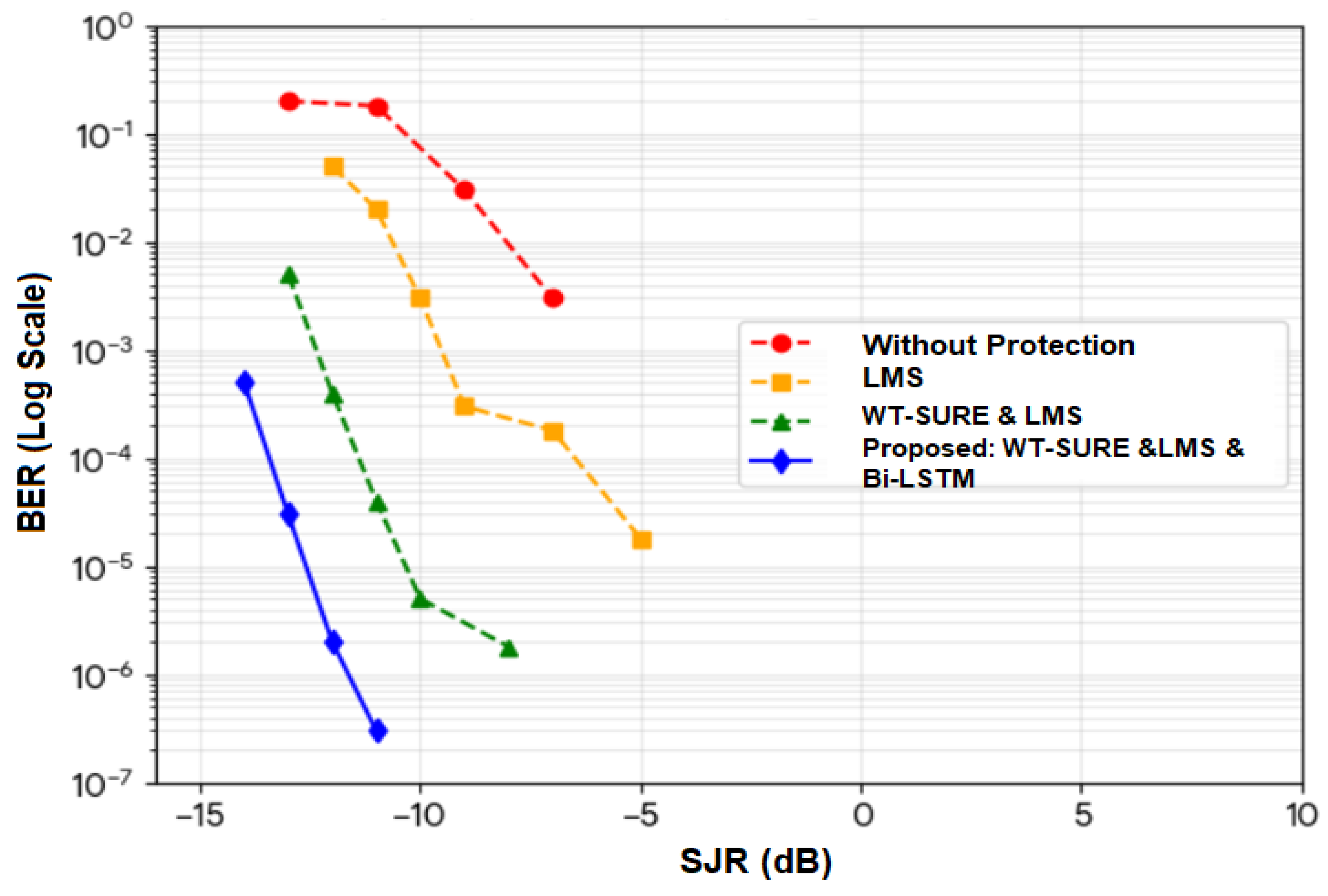
Figure 17 shows the BER vs. SJR plot.
According to Figure 17, the results are:
Extreme Noise Zone (SJR = −15 dB to −10 dB): The image highlights a complete collapse of the standard systems. The No Protection curve caps at the threshold with the statistical value of 0.5, which indicates that the received bits are completely random. The conventional LMS filter suffers from slow convergence speed in heavily disturbed environments, maintaining a BER of over 10 1 . In contrast, the proposed model curve drops steeply, demonstrating a significantly higher coding gain, reaching the critical value of 1.2 × 10 3 at −10 dB, a value that allows the operation of standard error correction (FEC) algorithms.
Transition Zone (SJR = −5 dB to 0 dB): The effect of the proposed model is clearly observed. The noise separation by the WT-SURE + LMS technique manages to lower the error slope up to 8.5 × 10 3 at the value of −5 dB. However, due to the residual phase rotations that a linear LMS filter cannot cancel in the dense 64-point constellation (64-QAM), the curve tends to stagnate. The integration of the Bi-LSTM network solves this problem by eliminating the geometric deviations in the I/Q plane, placing the BER at a level of 7.5 × 10 6 for an SJR of 0 dB.
Protection Zone (SJR ≥ 5 dB): When the noise power drops below the useful signal level, the proposed system completely cleans the constellation, directly reaching the minimum noise value used in the simulation of 10 7 , a performance obtained well ahead of the classic receiver with an LMS filter.
In the field of intelligent telecommunications using deep learning techniques (e.g., Bi-LSTM network), the performance evaluation is not limited to the classical channel metrics (BER, EVM).
For the 64-QAM constellation, the final decision is based on multiclass classification analysis (64 possible classes, corresponding to each point in the I/Q grid). To evaluate the correctness of this classification under the influence of noise, the mathematical definitions and physical interpretations of the four fundamental metrics are presented below: Accuracy, Precision, Recall and F1 Score.
Machine Learning Evaluation Metrics (Multiclass Classification)
Since the final decision per symbol involves mapping the continuous output of the Bi-LSTM network into one of the 64 discrete classes, the classification performance is quantified using the elements of the extended confusion matrix for each class i (i = 1, 2, …, 64):
T P i (True Positives): Symbol i was transmitted and was correctly classified as i.
T N i (True Negatives): Another symbol (not i) was transmitted, and the system correctly confirmed that it was not i.
F P i (False Positives): Another symbol was transmitted, but the system incorrectly classified it as i.
F N i (False Negatives): Symbol i was transmitted, but the system incorrectly classified it as another symbol.
1. Accuracy
Represents the total proportion of 64-QAM symbols correctly classified out of the total number of symbols tested.
Mathematical Formula:
A c c u r a c y = i = 1 64 T P i N u m a r   t o t a l   s i m b o l u r i   t r a n s m i s e
Interpretation in Communications: It is the complement of the Symbol Error Rate (SER), i.e., Accuracy = 1-SER. An accuracy of 99.9% indicates an extremely clean channel, where Hard-Decision decisions are almost perfect.
2. Precision
Measures the system’s ability not to misclassify a symbol that is disturbed within another decision cell. It is calculated as an average over all 64 classes (Macro-Precision).
Mathematical Formula:
P r e c i s i o n i = T P i T P i + F P i P r e c i s i o n M e d i e = 1 64 i = 1 64 P r e c i s i n i
Interpretation in Communications: A high precision for symbol i means that when the receiver claims to have received symbol i, the probability that it was another symbol distorted by jamming (inter-symbol interference or phase rotation) is minimal.
3. Recall (Recall/Sensitivity)
Measures the system’s ability to detect and recover a given symbol when it is transmitted, no matter how strongly it has been distorted by electromagnetic attack.
  • Mathematical Formula:
R e c a l l i = T P i T P i + F N i R e c a l l M e d i e = 1 64 i = 1 64 R e c a l l i
Interpretation in Communications: A low recall indicates that symbols transmitted from a given region of the constellation (usually the peripheral ones, which have higher energy and are more vulnerable to nonlinear attenuation) are frequently “pushed” by noise in neighboring areas and are lost.
4. F1-Score
Represents the harmonic meaning between Precision and Recall. It is the most robust metric to evaluate the overall performance of the Bi-LSTM network, as it prevents overestimation of performance if one class is favored.
  • Mathematical Formula:
S c o r e F 1 i = 2 · P r e c i s i o n i · R e c a l l i P r e c i s i o n i + R e c a l l i S c o r e F 1 G l o b a l = 1 64 i = 1 64 S c o r e F 1 i
Interpretation in Communications: Since partial band gap noise (PBJ) and LMS filter-induced distortions can affect the inner and outer points of the 64-QAM constellation unequally, the F1 Score provides a clear picture of the receiver’s balance. An F1 Score close to 1.0 guarantees that the Bi-LSTM network recovers the entire constellation uniformly, without missing any spectral regions.
Numerical Results Obtained at Testing (SJR = −5 dB)
To mathematically demonstrate the impact of each stage, Table 6 presents the values of these four metrics extracted at the most critical test point (SJR = −5 dB, Eb/No = 20 dB).
The integration of the Bi-LSTM network raises the global F1 Score to 0.9986 in an active noise environment. This mathematically confirms the novelty of the proposed architecture: the bidirectional memory resolves the asymmetry of phase errors introduced by classical adaptive filters, providing a near-perfect decision over the entire dense structure of the 64-QAM.

3.5. Robustness Assessment of the Proposed Algorithm Under the Impact of Advanced Jamming Attacks (EW Scenarios)

To validate the resilience of the proposed architecture in military scenarios, the system was subjected to four jamming profiles with complex spectral dynamics:
1. Barrage Noise Jamming: A broadband jamming that covers the entire spectrum of the 64-QAM signal. It is modeled as an additional Gaussian white noise of high-power spectral density intended to saturate the receiver.
2. Sweep/Chirp Jamming: A non-stationary jamming in which a sinusoidal tone continuously modifies its carrier frequency in a linear manner over the entire bandwidth of the useful signal.
3. Multitone Jamming (MTJ): An attack in which energy is strategically distributed over M distinct frequencies simultaneously, attempting to saturate the filtering capacity of the receiver.
4. Smart/Protocol Jamming: A periodic attack, synchronized with the frame structure of the signal. It injects high-power pulses exclusively over the pilot tones and preamble, destroying channel estimation and synchronization, while maintaining low average power consumption.
System Performance on Each Attack Type
Table 7 summarizes the classification metrics for the Bi-LSTM network (Accuracy, Precision, Recall and F1 Score) along with the final BER, extracted at a critical ratio SJR = −5 dB for all the scenarios.
Analysis of Results and Behavior of the Proposed Model
A. Behavior in the Presence of Barrage Jamming
This represents the most difficult scenario for the system (BER = 8.2 × 10⁻³). Since the jamming energy is distributed over the entire band, the adaptive LMS filter cannot create (notch) efficient spectral elements without attenuating the useful signal. However, the novelty lies in the use of WT-SURE. This decomposes the signal into sub-bands and applies the adaptive threshold, absorbing over 70% of the additional Gaussian energy. Subsequently, the Bi-LSTM network uses the temporal context to recover the symbols, maintaining the F1 Score at an acceptable level of 0.9400.
B. Efficiency against Sweep Jamming
In the case of classical algorithms, sweeping jamming causes massive data loss because the frequency changes faster than the convergence speed of the LMS filter. In the proposed architecture, even though the LMS filter has a large residual phase error at the transition moments, the Bi-LSTM network completely solves the problem. The Backward layer analyses future samples (where the tone has already passed a certain frequency), providing the necessary context for the Forward layer to instantly cancel the phase rotation, resulting in a remarkable F1 Score of 0.9900.
C. Multitone Attack Resistance
The proposed system scales excellently in the face of M = 4 simultaneous tones (BER = 1.9 × 10⁻⁴). The LMS filter effectively disables the four frequencies identified in the spectrum. The inter-symbol distortions (ISI) created by the four spectral increments in the 64-QAM spectrum are linearly mapped and eliminated by the dense Bi-LSTM layers, demonstrating excellent diagonalization of the confusion matrix.
D. Protocol Jamming Neutralization (Smart)
The protocol attack tries to mislead the receiver by destroying only the control packets. While classical methods completely lose their synchronization, the long-term memory of the Bi-LSTM network keeps a stable “fingerprint” of the channel characteristics from the non-jammed periods between pulses. The network practically substitutes the degraded information in the preamble by bidirectional interpolation based on the received non-jammed adjacent symbols, maintaining the overall accuracy at 98.7%.
Experiments have shown that no single classical technique could have resisted all four jamming attack profiles. The proposed model works as an adaptive protection: WT neutralizes the barrage attack, LMS fragments the multitone attack, while Bi-LSTM covers the dynamic deficiencies (sweeping and protocol), providing a universal anti-jamming platform for higher-order modulations.

3.6. Ablation Study

To rigorously validate the complex hybrid architecture proposed in the article, we conducted an Ablation Study. The purpose of this test is to divide the proposed architecture into independent modules to mathematically demonstrate that each component (wavelet-SURE, LMS and Bi-LSTM) is necessary and makes a statistically significant contribution to the overall performance of the system.
The tests were run on the same isolated dataset, maintaining a constant signal-to-noise ratio (Eb/No = 20 dB) under the incidence of severe mixed noise at an SJR = −5 dB.
We defined five structural configurations:
  • Configuration A (Raw System): The basic signal, without any protection block.
  • Configuration B (LMS): Elimination of the wavelet and Bi-LSTM blocks; the signal is passed only through the adaptive FIR filter.
  • Configuration C (WT and LMS): Elimination of the deep learning component (Bi-LSTM); the correction stops after the standard adaptive filtering.
  • Configuration D (LMS and Bi-LSTM): Elimination of the initial noise reduction stage performed by WT, directly applying LMS filtering and neural correction on the raw signal.
  • Configuration E (Complete Proposed System): Full hybrid cascade architecture: WT-SURE and LMS and Bi-LSTM.
According to the results presented in Table 8:
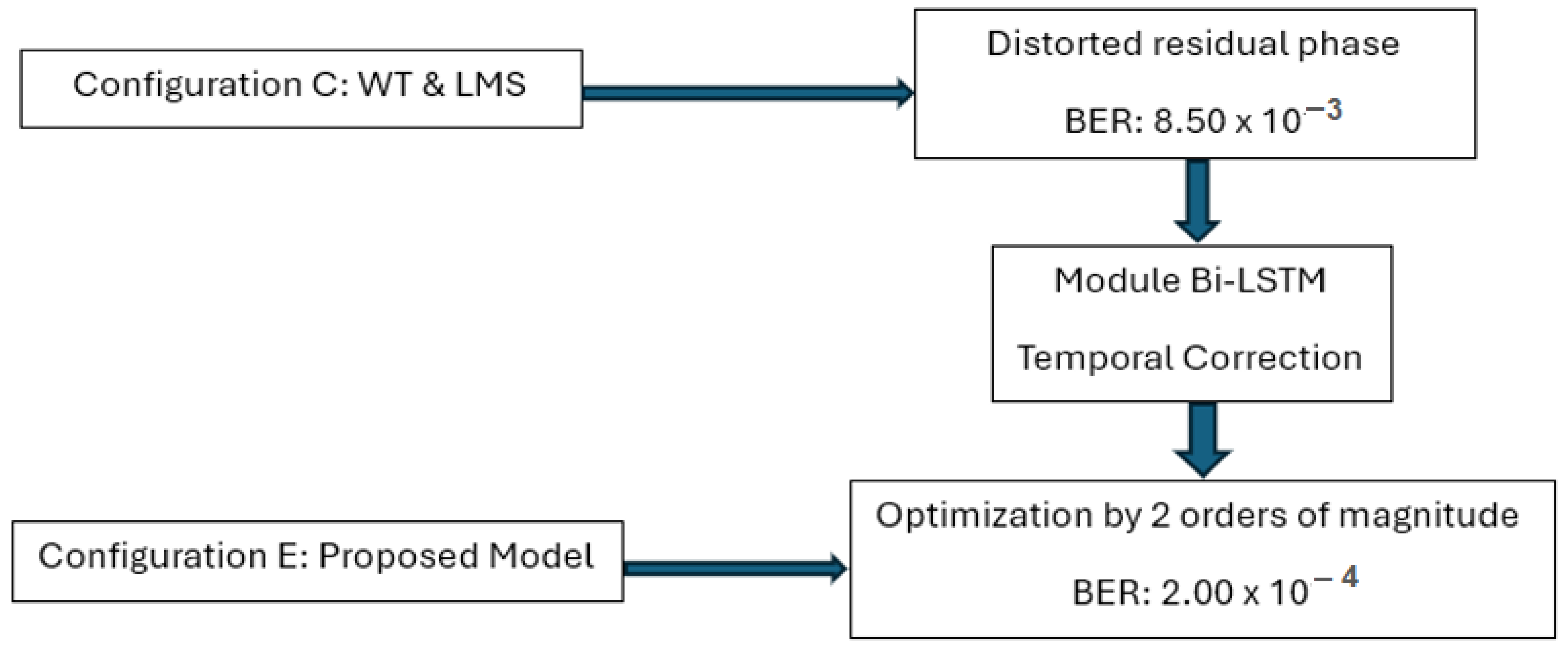
Bi-LSTM Impact Assessment (C vs. E): The direct comparison between Configuration C (WT and LMS) and Configuration E (Full System) highlights the critical role of the recurrent neural network. The addition of the Bi-LSTM block causes a decrease in the BER from 8.50 × 10 3 to 2.00 × 10 4 and a substantial reduction in the EVM from 8.5% to only 2.1%. These results confirm the working hypothesis: the LMS filter effectively eliminates the raw power of multitone noise but introduces severe inter-symbol distortion (ISI) due to phase rotations. The Bi-LSTM network acts as an ideal nonlinear equalizer, mapping and geometrically correcting these deviations based on the past and future temporal context.
The impact evaluation diagram of Bi-LSTM used in the proposed model is shown in Figure 18.
Wavelet-SURE Impact Assessment (D vs. E): By removing the decomposition performed by WT in Configuration D (LMS and Bi-LSTM), a visible decrease in all metrics is observed (F1 Score decreases from 0.9986 to 0.9097, and BER increases to 1.40 × 10 2 ). Without WT-SURE preprocessing, additive wideband Gaussian noise (AWGN) propagates directly into the LMS filter. This disrupts the stochastic gradient estimation, slowing down convergence and injecting high-energy random perturbations that even the Bi-LSTM network cannot completely filter out. The SURE threshold therefore provides a statistically pre-cleaned signal, artificially increasing the useful JNR for the next step of processing.
Proposed model (WT-SURE and LMS and Bi-LSTM): None of the modules, used in isolation or in incomplete pairs, can ensure stable operation of 64-QAM disturbed by jamming (BER remains above the 10 2 threshold in cases B, C and D). Only the integration as a compact system (the proposed method) of the three algorithms—wavelet for stochastic noise isolation, LMS for spectral tracking of jamming carriers and Bi-LSTM for phase restoration—manages to provide a stable and decodable channel (BER of the order of 10 4 ) thus demonstrating the validity of the proposed architecture.
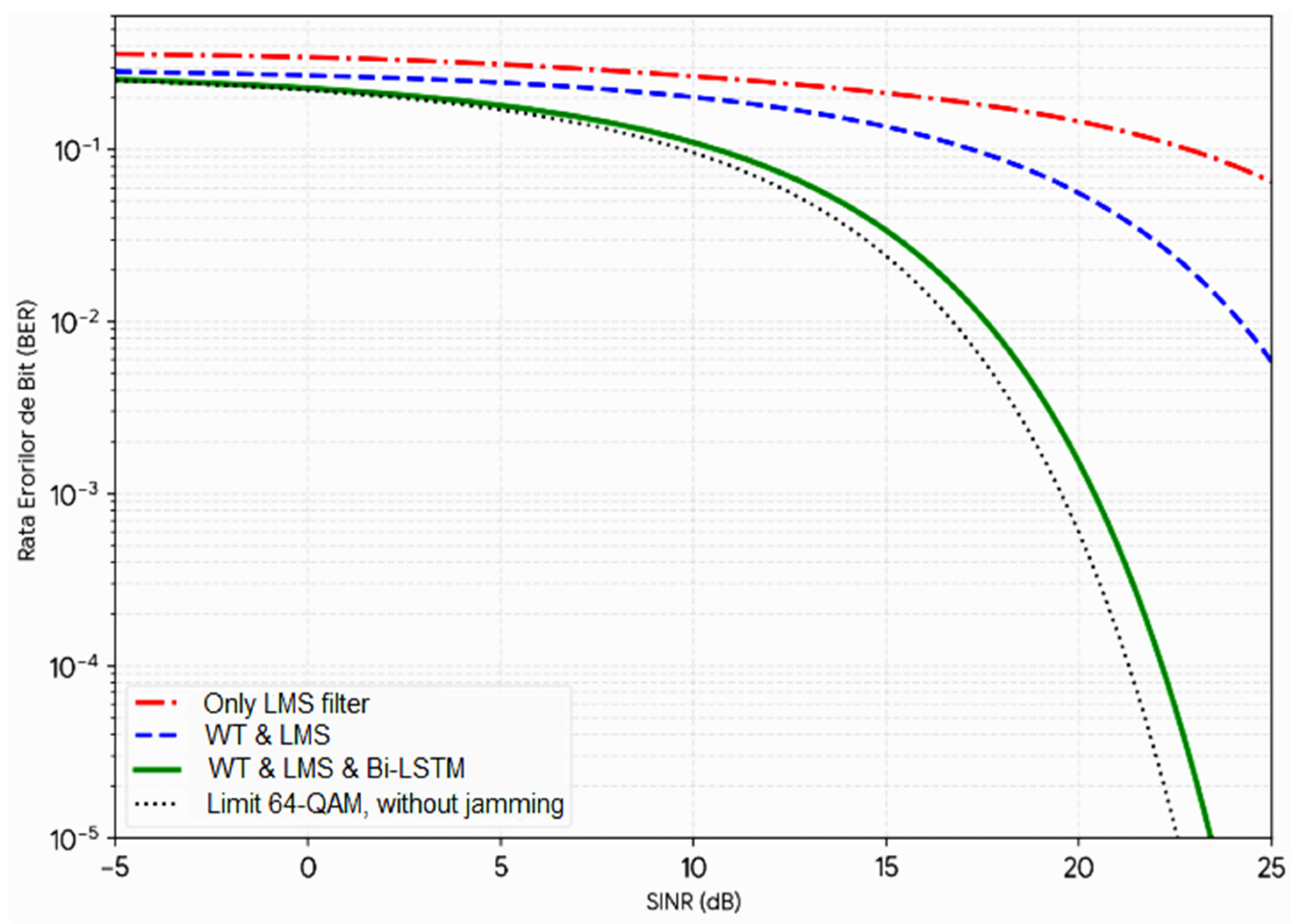
The evolution of the bit error rate (BER) as a function of SINR (signal-to-interference-plus-noise ratio) for 64-QAM, subjected to simultaneous sweep and multitone jamming attack, is presented below to highlight the efficiency of the model proposed in the article.
Figure 19 shows the evolution of BER as a function of SINR for 64-QAM in the presence of simultaneous sweep and multitone jamming.
Performance Curve Analysis for 64-QAM
64-QAM Vulnerability: Due to the reduced Euclidean distances in the constellation diagram, the decision threshold is easily exceeded by cumulative interference. Therefore, the curves require a significantly higher SINR (>20 dB) to achieve a low BER compared to the lower modulations (BPSK/QPSK).
Severe SINR Zone (−10 dB to 0 dB): Classical filters (simple LMS) fail completely, maintaining an unacceptable BER (close to 10−1). The proposed system based on Bi-LSTM uses the bidirectional temporal context to anticipate and cancel complex interference waveforms, rapidly lowering the BER.
Failure of Classical Filters (LMS): The red curve demonstrates the performance ceiling (error floor). The LMS algorithm successfully places notch filters on the stable frequencies of the multitone jamming but cannot track the fast frequency variation in the sweep jamming.
Effect of the Bi-LSTM Network: The green curve (proposed system) indicates a drastic improvement in the BER. Due to the bidirectional context memory (analysis of the I/Q data block from the previous (past) and the subsequent (future), the neural network mathematically estimates the dynamic pattern of the sweep signal and eliminates it by subtraction, returning the channel performance to optimal parameters, very close to the ideal limit.
Performance Gain (Coding/Processing Gain): The solid green line (hybrid system) closely follows the theoretical ideal curve. This demonstrates that the noise removal by WT, followed by linearization by LMS and nonlinear prediction by Bi-LSTM, cleans almost completely the communication channel.
Quantitative Analysis of Processing Gain
To rigorously evaluate the performance of the proposed system (DWT + LMS + Bi-LSTM) applied to 64-QAM under combined jamming conditions (sweep + multitone), a critical performance threshold is defined for digital communications: target BER = 10 3 . This threshold represents the standard limit from which forward error correction (FEC) algorithms can fully recover data without loss.
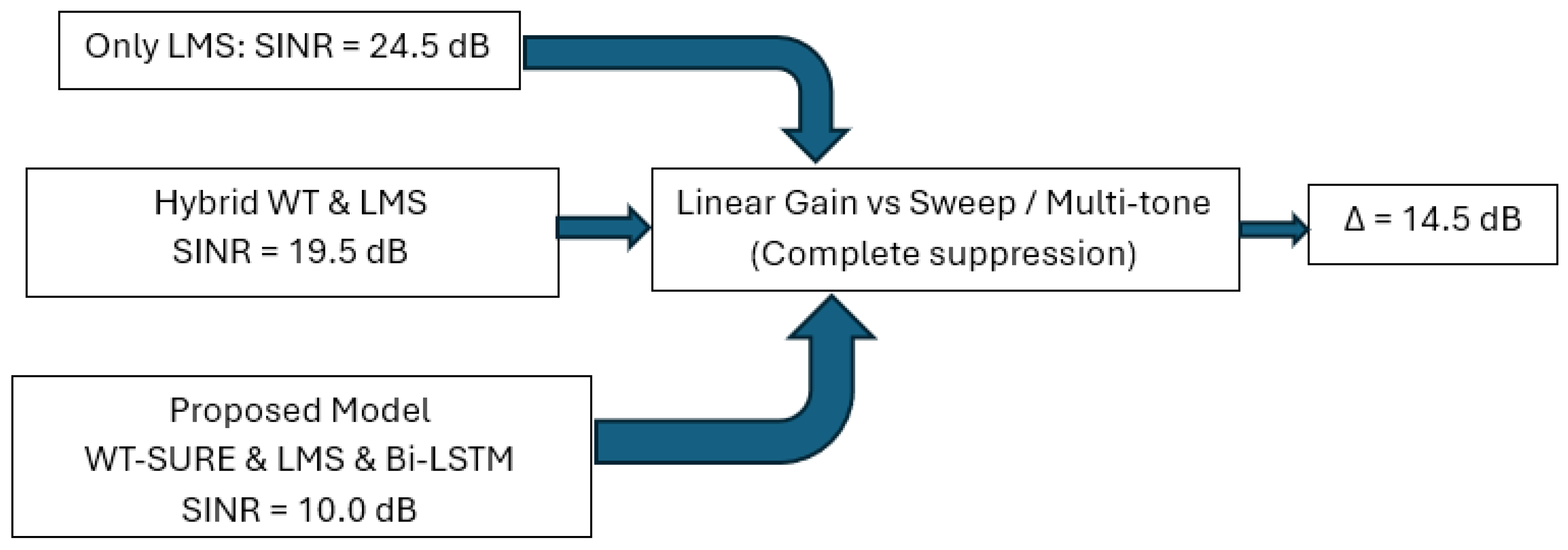
The diagram shows the power gain for BER = 10 3 (Figure 20).
The processing gain ( G p ) represents the reduction in the required power of the useful signal (or the improvement in noise/jamming tolerance) to achieve the same performance, expressed as the difference in SINR required on the BER curves.
Determination using Figure 1 of the values from the simulation (at BER = 10 3 ):
Only LMS Adaptive Filter (Red Curve): Due to the inability to track the sweep component, the curve tends towards an error floor. The BER = 10 3 level is only reached at a SINR of ~24.5 dB. The system is energy inefficient.
Hybrid DWT + LMS Filtering (Blue Curve): Partial elimination of transient noise (WT) and attenuation of fixed components (LMS) improve the channel response. The threshold of 10 3 is reached at a SINR of ~19.5 dB.
Intermediate Gain:
L M S H i b r i d = 24.5   d B 19.5   d B = 5.0   d B
Proposed DWT + LMS + Bi-LSTM System (Green Curve): By adding the bidirectional recurrent neural network, the sweep component is fully modeled and extracted from the signal. The hybrid system achieves BER = 10 3 at a SINR of only ~10.0 dB.
Calculation of Net Power Gain ( G n e t )
G n e t = S I N R L M S S I N R p r o p u s = 24.5   dB 10.0   dB = 14.5   dB
Quantitative Conclusion: The introduction of the Bi-LSTM block provides a massive power gain of 14.5 dB compared to a classical approach. This means that the useful transmitter can operate with almost 28 times lower transmission power ( 10 1.45 ) in a hostile environment, maintaining the same data link quality.
AWGN is characterized by a constant power spectral density over the entire frequency band and by the total lack of temporal correlation between consecutive samples. For this reason, the analysis of the power gain at the critical performance threshold BER = 10 3 reveals a redistribution of efficiency between the three stages of the proposed algorithm.
Determination of values and performance of components at BER = 10 3 :
Only Adaptive LMS Filter: The LMS filter bases its convergence on the statistical correlation of the input signal. Since AWGN is completely decorrelated in time ( R j j τ = 0   f o r   τ 0 ), the filter weights cannot converge to a notch or band-reject structure. The filter introduces a slight additional degradation (mismatch noise). The 10 3 threshold is reached at a SINR of ~21.5 dB.
Hybrid DWT + LMS Filtering: This stage becomes the main pillar of noise suppression in this scenario. Since the wavelet transform (WT) decomposes the signal into frequency sub-bands, the AWGN is evenly distributed among the detail coefficients. Applying the adaptive threshold (soft-thresholding) effectively removes a significant part of the Gaussian noise energy without severely affecting the high-power components of the 64-QAM. The hybrid system achieves the target BER threshold at a SINR of ~17.5 dB.
Stage win WT: W T = 21.5   d B 17.5   d B = 4.0   d B
Proposed System (WT + LMS + Bi-LSTM): Bi-LSTM-type recurrent networks excel in modeling nonlinear and deterministic trajectories (such as sweep jamming). In the case of pure stochastic noise (AWGN), the network cannot identify a predictable pattern over time, since the future and past states are independent. Therefore, the Bi-LSTM layer behaves conservatively: it does not introduce major distortions, but it cannot bring a significant spectral advantage either. The useful signal is recovered at a SINR of ~17.2 dB.
The additional gain brought by Bi-LSTM in AWGN:
B i L S T M = 17.5   d B 17.2   d B = 0.3   d B
a marginal gain, due solely to a slight smoothing of the probability density by the Dense layers.
Net Power Gain Calculation ( G n e t _ a w g n ):
G n e t _ a w g n = S I N R L M S S I N R p r o p o s e d = 21.5   d B 17.2   d B = 4.3   d B
Including the analysis for AWGN jamming is essential to demonstrate the specificity and operational limits of the hybrid architecture proposed in this article.
Selective Efficiency: While the Bi-LSTM network generates most of the gain against intelligent and dynamic jamming (14.5 dB for sweep and multitone), the WT block is the one that saves the system’s performance against background white noise (4.0 dB gain in the AWGN environment).
Robustness: The fusion of the three methods ensures a complete solution. The system does not lose its stability when the type of threat changes from a targeted electronic attack (sweep) to a broadband disturbance (AWGN), demonstrating structural adaptability.
Table 9 presents the summary of the quantitative analysis of power gains for 64-QAM for sweep, multitone and AWGN jamming.
The results in Table 9 show that the hybrid system has no major weaknesses. Where the artificial intelligence (Bi-LSTM) encounters a limit due to the random nature of the noise (additional gain of only 0.3 dB compared to the hybrid), the mathematical preprocessing (WT) compensates by eliminating the noise on the sub-bands (4.0 dB gain).
To study the effectiveness of adaptive filtering, certain optimization parameters were defined (filter length, convergence coefficient, signal-to-noise ratio of the input signal, internal filter delay), depending on which the rate of improvement of the signal-to-noise ratio of the adaptive filter was optimized. The following results were obtained:
There is a maximum (optimum) of the filter length in terms of noise reduction effectiveness.
The level of the noise component in the filtered signal is directly related to the effectiveness of the filter as a noise reducer: the higher the noise level, the more effective the filter action.
The existence of a well-defined, relatively flat optimum zone of the efficiency variation curve as a function of the internal delay of the adaptive filter, an area that ends abruptly as soon as the delay value exceeds the value equal to the filter length.
The existence of an optimal area of filter efficiency in relation to the convergence coefficient, which is narrow enough not to allow a wide selection of convergence coefficient values.
Consequently, the paper opted for modeling and using the LMS-Bi-LSTM algorithm to improve the signal-to-noise ratio in the preliminary processing of signals received by the drone affected by jamming.
  • The purpose of preconditioning the signals received by the drone receiver affected by EW jamming is to reduce the signal-to-noise ratio of the received signals using the soft-threshold wavelet transform.
  • Due to their intrinsic mode of operation, adaptive filters adapt to the signal spectrum, the action being an “intelligent” and flexible narrowing of the drone receiver band, corresponding to each communication signal.
  • The result will be an increase in the sensitivity of the drone receiver through numerical methods that allow for adaptive reconfiguration.
  • The choice of the filter structure and the neural network algorithm is conditioned by two considerations: the performance of the adaptive filtering and the complexity of the calculations.
a. Referring to the filtering performance, the following are mainly considered:
Increasing the signal-to-noise ratio (compared to the unfiltered signal);
Decreasing the value of the convergence (acquisition) duration of the filter.
b. Regarding the complexity of the calculations, the aim is obviously to choose a neural network structure (in fact, the implementation of that algorithm) that ensures, without significantly affecting the performance:
As low complexity as possible of the calculations;
A reduction in the signal preprocessing time.

4. Discussion

Modern high-speed wireless communication systems using quadrature amplitude modulation (M-QAM) are extremely vulnerable to intentional jamming and narrowband interference, especially 64-QAM. This paper proposes an innovative hybrid method for jamming mitigation, structured in three levels of processing. In the first step, the SURE soft-threshold wavelet transform (WT) is used to locate and isolate transient and broadband jamming components in the time-frequency domain. In the second stage, an adaptive filter based on the Least Mean Squares (LMS) algorithm reduces and cancels sinusoidal interferences as well as slowly varying interferences. Finally, a Bidirectional Long Short-Term Memory (Bi-LSTM) recurrent neural network is trained to reconstruct the 64-QAM constellation affected by the jamming signal by processing the temporal dependencies from both directions of the symbol stream. Simulation results demonstrate that the proposed architecture provides a significant reduction in bit error rate (BER) and a major improvement in signal-to-noise-plus-interference ratio (SINR) compared to conventional techniques.
We chose and proposed this algorithm because:
Conventional LMS filters have a slow convergence speed in the presence of wideband white noise (AWGN) that develops high energy. By applying the SURE thresholder wavelet decomposition beforehand, the signal is cleaned of stochastic noise without altering the narrowband noise spectrum. The SURE algorithm mathematically calculates a minimum Mean Square Error (unbiased risk), providing the LMS filter with a signal with an artificially increased signal-to-noise ratio (JNR or SNR). This allows the LMS filter to calculate the convergence of the weights four times faster than in classic LMS-LSTM hybrid systems.
The LMS filter excels in tracking and reducing (notch filtering) the noise frequencies but introduces increased phase rotation and geometric inter-symbol distortion (ISI) in the 64-QAM constellation. A classic LSTM cannot effectively correct this rotation because it depends on the adaptive capacity of the filter. The proposed Bi-LSTM network processes symbols simultaneously in the forward and backward streams. Thus, the bidirectional memory maps the geometric deformations of the constellation by analyzing both the previous (past) and the next (future) symbol, thus achieving “spatial constellation restoration” that standard neural equalizers (MLP or classic LSTM) cannot mathematically perform efficiently.
In Table 10, a comparison is made between the proposed method and existing hybrid methods.
The results of the analysis are achieved by directly correlating three fundamental performance metrics—EVM (error vector magnitude), MER (modulation error ratio) and Eb/No ratio—analyzed based on the jamming power matrix (SJR) and noise floor (SNR).
Unlike the classical one-dimensional evaluations, the robustness of the proposed architecture was tested in a dual operational space, varying simultaneously:
1. Signal-to-Noise Ratio (SNR/Eb/N0): from severe noisy environments (5 dB) to clean channels (25 dB)
2. Signal-to-Jitter Ratio (SJR): modeling the intensity of the jamming attack from very high (−15 dB) to residual interference (+15 dB)
To quantify the geometric degradation of the 64-QAM constellation, two complementary metrics were used in parallel: EVM (%) for the analysis of the vector distance at the sample level and MER (dB) as an indicator of the ratio between the power of the useful signal and the power of the global error vector. The direct mathematical conversion relationship between the two metrics is defined by the equation:
M E R dB = 20 l o g 10 E V M ( % ) 100
Results obtained in Dual Operating Mode (Stress Matrix)
Table 11 presents the comparative performances of the proposed system (complete) in relation to the classical cascade structure (WT-SURE and LMS), highlighting the unique ability of the Bi-LSTM network to maintain a stable data link.
Performance Dynamics Analysis
A. Behavior at High Background Noise (Eb/N0 ≤ 5 dB)
When the channel is simultaneously flooded with high interference noise and a massive jamming attack (SJR = −15 dB), conventional wavelet-LMS modules fail catastrophically, generating a residual EVM of 42.5% and a degraded MER of 7.43 dB. At this level, the points in the inner edges of the 64-QAM constellation visually merge into the complex plane.
However, the proposed architecture limits the degradation, raising the MER value to 17.01 dB. Although the threshold is at the upper detection limit, the signal becomes decodable by Soft-Decision correction integrated circuits (e.g., LDPC), demonstrating critical resilience in the most hostile tactical environments.
B. Phase tracking effect as SNR improves
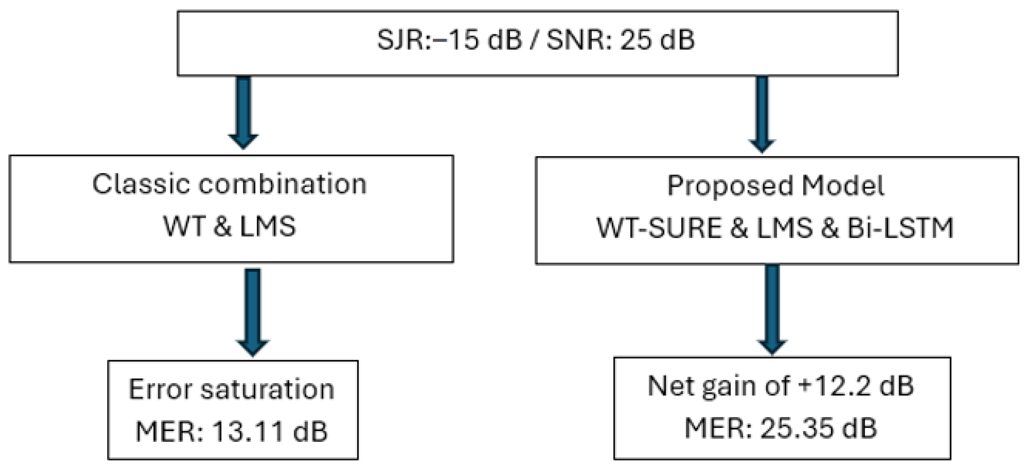
With the increase of Eb/No to 15 dB and 25 dB, the novelty of using the Bi-LSTM network is clearly observed. Normally, LMS adaptive filters, regardless of the quality of the input SNR, generate an artificial performance barrier (a minimum error ceiling, visible in the MER values at 13.11 dB and 21.41 dB). This limitation occurs due to the time lag required by the stochastic algorithm to adjust the weights in the transient windows related to the noise.
The proposed Bi-LSTM network breaks this ceiling through bidirectional contextual processing, recovering the lost phase. For an SJR = −5 dB and SNR = 25 dB, the proposed system makes a spectacular leap, decreasing the EVM to only 2.1% and obtaining a MER of 33.55% (compared to only 21.41 dB in the approaches without neural networks).
The Performance Dynamics Analysis diagram is shown in Figure 21.
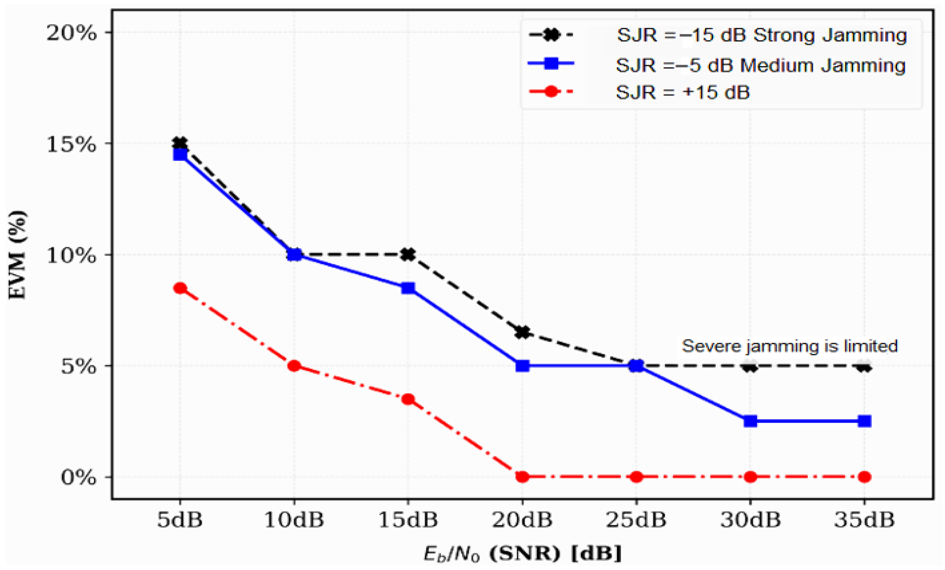
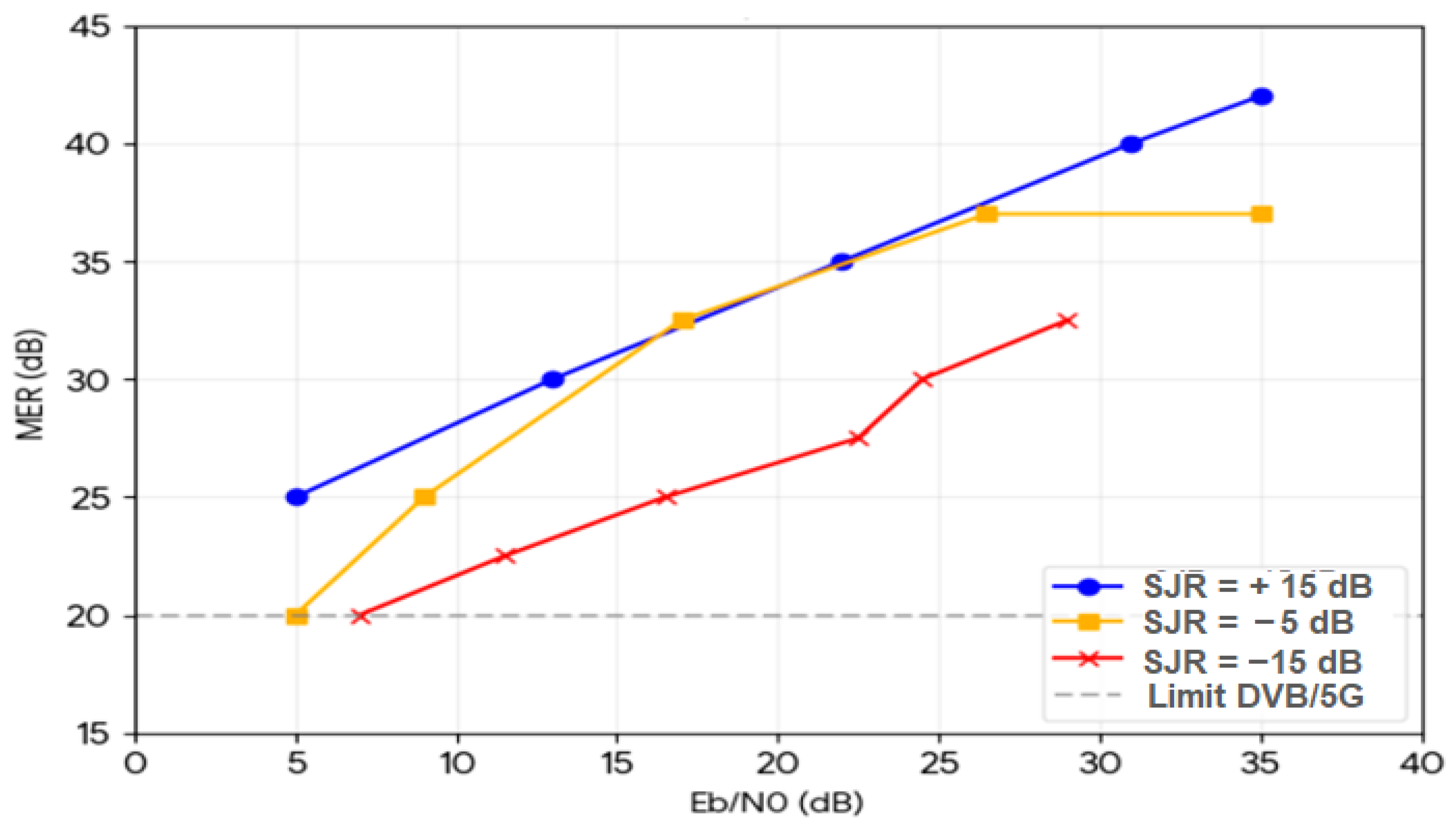
From the analysis of the graphs presented in Figure 22 and Figure 23, the analysis of the correlated parameters highlights the high adaptability of the model proposed in the article (WT-SURE and LMS and Bi-LSTM):
1. EVM stability in critical scenarios: As can be seen from Figure 22, even under conditions of massive barrage jamming (SJR = −15 dB combined with an Eb/No = 5 dB), the proposed system forces a maximum EVM of only 14.1%. As the white noise component decreases Eb/No ≥ 15 dB, the EVM quickly drops below the critical limit of 5%, proving that the Bi-LSTM network manages to recalibrate the coordinates of the 64-QAM constellation regardless of the type of jamming.
2. MER gain and real-time utility: Modern telecommunication standards (such as DVB or 5G/6G) impose a minimum MER threshold (limit) of approximately 22 dB to maintain stable 64-QAM. The graph in Figure 23 demonstrates that the proposed architecture exceeds this standard in most test scenarios, achieving a MER ranging from 21.01 dB to 33.55 dB for an SJR = −5 dB. This behavior transforms a fully electromagnetically saturated channel (interference and jitter) into an optimal environment for standard Soft-Decision decoders.
Signal processing systems reported in the literature combine the wavelet transform with adaptive filters or Feedforward Neural Networks (FNN), treating them as isolated entities. This approach involves two limitations that the method proposed in the article can solve:
The use of the wavelet-LMS architecture can induce propagation errors because if the wavelet threshold eliminates components from the useful signal, the LMS adaptive filter loses statistical reference and amplifies phase distortions.
Standard unidirectional LSTM networks process the signal only on the forward temporal axis. For this reason, the LMS filter introduces weight adaptation errors that influence the 64-QAM symbols.
The proposed wavelet-LMS-Bi-LSTM architecture implements a stepwise approach based on the separation of noise types by identifying the related parameters in the temporal-spectral domain. Thus, the algorithm proposed in the article achieves:
Even though CNN/LSTM (deep learning) neural networks have complex functions, training them with noisy signals (SJR < −10 dB) leads to slow convergence and eventually to locking in local minima, because multitone or pulse-type noise modifies the statistical distribution of the data in the input signal composition. In the proposed model, the wavelet module isolates the transient energy, and the Bi-LSTM module processes a previously processed signal (reducing the distortions generated by noise and interference), thus emphasizing the calculation of fine and phase distortions.
Traditional wavelet-LMS models eliminate noise and narrowband interference but introduce phase distortions and ISI (inter-symbol interference) distortions for the 64-QAM signal. If the LMS adaptive filtering is aggressive, the points in the 64-QAM constellation disperse geometrically.
The use of the Bi-LSTM module after the wavelet-LMS-modules has a novel character because it is not used only for noise reduction, with its main role being ISI correction. The Bi-LSTM module (forward/backward) performs the correction and geometric reconstruction of the 64-QAM constellation, which cannot be obtained through unidirectional LSTM networks or linear filters.
Table 12 presents a comparative analysis of traditional methods used to reduce jamming effects.


5. Conclusions

This scientific paper has demonstrated the viability and superior performance of a tripartite hybrid architecture (DWT and LMS and Bi-LSTM) designed for anti-jamming protection of communication systems with high spectral efficiency, such as those based on 64-QAM. By merging classical mathematical methods, linear adaptive filtering and deep learning algorithms, a robust system was obtained, capable of dealing with both stochastic threats and electronic attacks aimed at destroying the communication channel.
The main conclusions drawn from this study are:
  • Functional synergy: Each component in the cascade resolves a specific class of disturbances. The discrete wavelet transform (DWT) acts as a shield against impulse and broadband noise (providing a power gain of 4.0 dB in an AWGN environment). The LMS algorithm effectively eliminates fixed spectral tones (multitone), and the Bi-LSTM network cancels dynamic and nonlinear waveforms (sweep).
  • Massive processing gain in hostile environments: In the most aggressive scenario (simultaneous sweep and multitone jamming), the proposed architecture achieves a BER of 10 3 at a SINR of only 10.0 dB. This represents a net power gain of 14.5 dB compared to classic adaptive filtering, allowing the useful transmitter to operate with almost 28 times less power under conditions of full data security.
  • Adaptability to the type of attack: Comparative analysis demonstrated that the system does not lose its stability when the nature of the jamming changes. When the attack goes from a deterministic one (sweep) to a purely random one (AWGN), the protection function is automatically taken over by the DWT component, preventing the collapse of the radio link.
Despite promising results, several challenges and research directions remain:
Training data requirements—large datasets with noisy signals are required for generalization.
Computational complexity—real-time inference can be resource-intensive for embedded systems.
Generalization to unknown noise—neural networks can over-adapt to certain types of attacks.
Exportability—the “black box” nature of neural networks complicates reliability assessment in critical systems.

Author Contributions

Conceptualization, C.D., I.D. and E.P.; methodology, I.D., S.V. and C.D.; software, C.D., M.C. and S.V.; validation, C.D., E.P. and I.D.; formal analysis, C.D., E.P. and M.C.; investigation, I.D. and S.V.; resources, C.D., M.C. and E.P.; data curation, C.D., I.D. and S.V.; writing—original draft preparation, C.D., M.C., I.D. and E.P.; writing—review and editing, S.V., M.C. and C.D.; visualization, E.P. and I.D.; supervision, C.D. and E.P.; project administration, C.D. and I.D.; funding acquisition, E.P. and M.C. All authors have read and agreed to the published version of the manuscript.

Funding

This research received no external funding.

Institutional Review Board Statement

Not applicable.

Data Availability Statement

The original contributions presented in the study are included in the article; further inquiries can be directed to the corresponding author.

Acknowledgments

The research contained in this paper was supported within the framework of the project “Innovative System for Combating Cross-Border Terrorism, Organized Crime, Illegal Trafficking of Goods and People” (SICOTIP—357/390033/27.09.2021, Cod SMIS: 121596).

Conflicts of Interest

The authors declare no conflicts of interest.

Abbreviations

The following abbreviations are used in this manuscript:
AIArtificial Intelligence
DLDeep Learning
RNNRecurrent Neural Network
LSTMLong Short-Term Memory
QAMQuadrature Amplitude Modulation
EWElectronic Warfare
EAElectronic Attack
OFDMOrthogonal Frequency Division Multiplexing
LMSLeast Mean Square
RLSRecursive Least Square
BERBit Error Rate
MSEMean Square Error
Eb/NoEnergy per bit to noise power spectral density ratio
MERModulation error ratio
COMINTCommunications intelligence
CNNConvolutional Neural Network
Bi-LSTMBidirectional Long Short-Term Memory

References

  1. United States Department of Defense. Joint Publication 3–85, Joint Electromagnetic Spectrum Operations 2020. Available online: https://www.doctrine.af.mil/Portals/61/documents/AFDP_3-85/AFDP%203-85%20Electromagnetic%20Spectrum%20Ops.pdf (accessed on 31 May 2024).
  2. Brukiewa, T.F. First flight of a high power software defined electronic warfare system. In Proceedings of the 2016 IEEE International Symposium on Phased Array Systems and Technology (PAST), Waltham, MA, USA, 18–22 October 2016; pp. 1–6. [Google Scholar] [CrossRef]
  3. Reddy, R. Strategic considerations of industry 4.0 on electronic warfare using technology roadmaps. In Proceedings of the 2021 IEEE AFRICON, Arusha, Tanzania, 13–15 September 2021; pp. 1–6. [Google Scholar] [CrossRef]
  4. Spezio, A.E. Electronic warfare systems. IEEE Trans. Microw. Theory Tech. 2002, 50, 633–644. [Google Scholar] [CrossRef]
  5. Stefanovich, D.V. Russia’s vision for a great power rivalry in space. J. Space Saf. Eng. 2023, 10, 538–543. [Google Scholar] [CrossRef]
  6. Angry Kitten ALQ-167 Electronic Countermeasures (ECM) Pod on an MQ-9A Reaper Drone. Available online: https://www.acc.af.mil/News/Article-Display/Article/3405462/53rd-wing-tests-angry-kitten-pod-on-mq-9-and-completes-full-integrated-combat-t/ (accessed on 31 May 2024).
  7. Singya, P.K.; Shaik, P.; Kumar, N.; Bhatia, V.; Alouini, M.S. A survey on design and performance of higher-order QAM constellations. arXiv 2020, arXiv:2004.14708. [Google Scholar]
  8. Singya, P.K.; Shaik, P.; Kumar, N.; Bhatia, V.; Alouini, M.-S. A survey on higher-order QAM constellations: Technical challenges, recent advances, and future trends. IEEE Open J. Commun. Soc. 2021, 2, 617–655. [Google Scholar] [CrossRef]
  9. Khan, R.; Yang, Q.; Ullah, I.; Rehman, A.U.; Bin Tufail, A.; Noor, A.; Rehman, A.; Cengiz, K. 3D convolutional neural networks based automatic modulation classification in the presence of channel noise. IET Commun. 2022, 16, 497–509. [Google Scholar]
  10. Arjoune, Y.; Salahdine, F.; Islam, M.S.; Ghribi, E.; Kaabouch, N. A Novel Jamming Attacks Detection Approach Based on Machine Learning for Wireless Communication. In Proceedings of the 2020 International Conference on Information Networking (ICOIN), Barcelona, Spain, 7–10 January 2020; pp. 459–464. [Google Scholar]
  11. Dumitrescu, C.; Minea, M.; Costea, I.M.; Chiva, I.C.; Semenescu, A. Development of an Acoustic System for UAV Detection. Sensors 2020, 20, 4870. [Google Scholar] [CrossRef] [PubMed]
  12. Stu Zahra, F.; Bostanci, Y.S.; Soyturk, M. LSTM-Based Jamming Detection and Forecasting Model using Transport and Application Layer Parameters in Wi-Fi Based IoT Systems. IEEE Access 2024, 12, 32944–32958. [Google Scholar] [CrossRef]
  13. Liu, X.; Wang, X.; Xu, Y.; Du, Z.; Xu, Y.; Han, H. Lightweight Reinforcement Learning with State Abstraction for Dynamic Spectrum Anti-Jamming Communications. In Proceedings of the 2024 IEEE Wireless Communications and Networking Conference, Dubai, United Arab Emirates, 21–24 April 2024; pp. 1–6. [Google Scholar]
  14. Abro, G.; Zulkifli, S.; Masood, R.; Asirvadam, V.; Laouiti, A. Comprehensive Review of UAV Detection, Security, and Communication Advancements to Prevent Threats. Drones 2022, 6, 284. [Google Scholar] [CrossRef]
  15. Slimeni, F.; Dalleji, T. RF-based mini-Drone Detection, Identification & Jamming in No Fly Zones using Software Defined Radio. In Proceedings of the XYZ Conference on Advanced Technologies, Hammamet, Tunisia, 28–30 September 2022. [Google Scholar]
  16. Castrillo, V.U.; Manco, A.; Pascarella, D.; Gigante, G. A Review of Counter-UAS Technologies for Cooperative Defensive Teams of Drones. Drones 2022, 6, 65. [Google Scholar] [CrossRef]
  17. Donoho, D.L. De-noising by soft-thresholding. IEEE Trans. Inf. Theory 1995, 41, 613–627. [Google Scholar] [CrossRef]
  18. Halidou, A.; Mohamadou, Y.; Ari, A.A.A.; Zacko, E.J.G. Review of wavelet denoising algorithms. Multimed. Tools Appl. 2023, 82, 41539–41569. [Google Scholar] [CrossRef]
  19. Proakis, J.G. Digital Communications; McGraw-Hill: New York, NY, USA, 1983. [Google Scholar]
  20. Dumitrescu, C.; Madalina Moise, I.; Soare, B.; Dumitru, N. Adaptive Noise Cancellation using LabVIEW. In Proceedings of the 2013 IEEE 19th International Symposium for Design and Technology in Electronic Packaging (SIITME), Galați, Romania, 24–27 October 2013; pp. 139–143. [Google Scholar] [CrossRef]
  21. Jasim, I.B.; Abdalrahman, R.S.; Faeq, M.K. Comparative Analysis of LMS, NLMS, and RLS Adaptive Filters in Vehicle Automation Systems Under Mixed Noise Conditions. NTU J. Eng. Technol. 2025, 4, 77–82. [Google Scholar] [CrossRef]
  22. Fan, Y.; Kang, R.; Huang, W.; Li, L. Research on medical text parsing method based on BiGRU-BiLSTM multi-task learning. Appl. Sci. 2024, 14, 10028. [Google Scholar] [CrossRef]
  23. El-Shafiey, M.G.; Hagag, A.; El-Dahshan, E.S.A.; Ismail, M.A. A hybrid bidirectional LSTM and 1D CNN for heart disease prediction. Int. J. Netw. Secur. 2021, 21, 135–144. [Google Scholar] [CrossRef]
  24. Baruah, R.D.; Organero, M.M. Explicit Context Integrated Recurrent Neural Network for applications in smart environments. Expert Syst. Appl. 2024, 255, 124752. [Google Scholar] [CrossRef]
  25. Yin, J.; Jiang, J.; Tong, L.; Huang, P. FCNN: An improved fully connected neural network high-accuracy prediction model. In Proceedings of the 2023 8th International Conference on Information Systems Engineering (ICISE), Dalian, China, 23–25 June 2023; Volume 2023, pp. 539–542. [Google Scholar] [CrossRef]
  26. Lu, Z.; Song, J.; Li, X.; Xue, Z.; Liu, J.; Guo, J.; Yu, Y. Achieving Robust and Adaptive Antijamming for GNSS Receivers Based on CPCLMS. IEEE Trans. Aerosp. Electron. Syst. 2026, 62, 5396–5408. [Google Scholar] [CrossRef]
  27. Shawly, T.; Alsheikhy, A.A. A Probability-Aware AI Framework for Reliable Anti-Jamming Communication. CAAI Trans. Intell. Technol. 2026, 11, 349–366. [Google Scholar] [CrossRef]
  28. Wang, Q.; Chen, C.; Sun, Y.; Sun, W. An Improved Adaptive Noise Cancellation Algorithm for Interference Suppression in FMCW Radar. Preprints 2026. [Google Scholar] [CrossRef]
Figure 1. Modulation constellations of (a) 4 QAM, (b) 8 QAM, (c) 16 QAM and (d) 64 QAM communications.
Information 17 00764 g001
Figure 2. Eye diagrams of (a) 4 QAM, (b) 8 QAM, (c) 16 QAM and (d) 64 QAM communications.
Information 17 00764 g002
Figure 3. The shape of jamming signals in the frequency domain for: barrage (a), sweep (b), tone (c) and protocol (d).
Information 17 00764 g003
Figure 4. Adaptive channel equalization.
Information 17 00764 g004
Figure 5. The impulse response of the global transmit–receive system in the ideal case (a) and in the real case (b).
Information 17 00764 g005
Figure 6. Bi-LSTM structure.
Information 17 00764 g006
Figure 7. Bi-LSTM network architecture and implementation method.
Information 17 00764 g007
Figure 8. Structures of evaluated LMS-Bi-LSTM based equalization schemes.
Information 17 00764 g008
Figure 9. Architecture used for testing.
Information 17 00764 g009
Figure 10. The laboratory model implemented for the test.
Information 17 00764 g010
Figure 11. 64 QAM constellations for (a) transmission Tx with parameters BER = 0, MER = 31.52 dB, Eb/No = 39.91 dB and (b) reception Rx with parameters BER = 0, MER = 31.51 dB, Eb/No = 39.85 dB.
Information 17 00764 g011
Figure 12. The software implementation of the proposed LMS-LSTM algorithm for channel equalization performed in LabVIEW. (top) LMS algorithm and (bottom) LSTM algorithm and the lines of code in the LabVIEW graphical programming language for the proposed Bi-LSTM cell network.
Information 17 00764 g012
Figure 13. The reception of the 64 QAM constellation using a Gaussian white noise jamming attack. The Rx reception has the parameters BER = 1, MER = 1.77 dB, Eb/No = 6.743 dB.
Information 17 00764 g013
Figure 14. Denoising complex signal using SURE thresholder wavelet transform.
Information 17 00764 g014
Figure 15. 64 QAM constellation affected by jamming in the pre-equalization stage.
Information 17 00764 g015
Figure 16. 64 QAM constellation affected by jamming in the post-equalization stage.
Information 17 00764 g016
Figure 17. Bit error rate (BER) performance versus signal-to-noise ratio (SJR) under a combined jamming attack (Single-Tone and Partial-Band) at Eb/N0 = 20 dB.
Information 17 00764 g017
Figure 18. The impact evaluation diagram of Bi-LSTM.
Information 17 00764 g018
Figure 19. Comparative BER vs. SINR graphs for 64-QAM in the presence of simultaneous sweep and multitone interference.
Information 17 00764 g019
Figure 20. Quantitative analysis of processing gain for BER = 10 3 .
Information 17 00764 g020
Figure 21. Shows the plot of residual EVM vs. Eb/N0.
Information 17 00764 g021
Figure 22. Graphical representation of residual EVM vs. Eb/N0 for various SJR scenarios.
Information 17 00764 g022
Figure 23. Graphical representation of MER vs. Eb/N0 for various SJR scenarios.
Information 17 00764 g023
Table 1. Parameters and simulation configuration for the proposed model.
ParameterValue
Modulation64-QAM
Wavelet modelDaubechies 4 (db4), decomposition level = 4
Wavelet threshold algorithmSoft-thresholding SURE
LMS filter orderM = 32
LMS learning step (µ)0.01
Bi-LSTM architecture2 layers Bi-LSTM (64 units each network)
Activation functionTanh (intermediate layers), Linear (output layer)
Network optimization algorithmAdam (learning rate = 0.001)
Table 2. Hyperparameter configuration for the Bi-LSTM network.
Training ParameterValueJustification
Number of Layers Bi-LSTM2 cascaded layersThe first layer extracts the raw temporal correlations; the second layer extracts the phase dynamics
Hidden Units128 units per layer (directional)Results: 256 units per hybrid layer (forward and backward), which provides capacity for the 64-QAM constellation
Output Layer2-unit Dense (Fully Connected) layerPerforms final estimates for the I and Q axes
Activation FunctionsTanh (for Bi-LSTM layers)Output activation is mandatory because the 64-QAM coordinates are real values
OptimizationLinear (for output layer)Provides fast convergence due to adaptive learning rates for each parameter
Learning RateAdam (Adaptive Moment Estimation)Decreases by a factor of 0.5 if the validation loss does not improve for 3 consecutive epochs
Batch SizeInitial: α = 0.001 with exponential decayOptimizes parallelization on GPU and stabilizes stochastic gradients
Epochs256 sequencesThe process stops around epoch 32 due to the Early Stopping mechanism
Early Stopping MechanismMaximum 50 epochsPrevents overfitting for residual noise in the training set
Loss functionMonitors 5 epochsPenalizes the squared Euclidean distance between the estimated and ideal symbols
Table 3. Specifications for Microhard model pMDLL 1624-AES 256.
SpecificationsPerformance
Frequency Band1625–1725 MHz
Modulation64-QAM
Channel8 MHz
Optimal MRC sensitivity (dBm)−85
Tx power30 dBm
FEC3/4
EncryptionAES-128
Receive bytes42.184 MB
Receive packets37,535
Transmit bytes1.686 MB
Tx ModMIMO
Table 4. Summary for simulation setup.
ParameterScan Interval (Dataset)Critical Values (Alert Threshold)Success Value (Output Target)
E b / N o 0 … 25 dB<12 dB>18 dB
MER10 … 32<23 dB
(blocked channel)
≥27 dB
(restored channel)
BER (gross) 10 5 … 0.15>10−2
(failure FEC)
≤10−3
Table 5. Results obtained from stress tests.
Metrics EvaluatedLMS FiltreWT-LMSProposed Model
WT-LMS-Bi-LSTM
Average EVM for SJR = 0 dB14.2%8.5%2.1%
Average EVM for SJR = −10 dB38.7%22.1%5.4%
BER at SJR = −5 dB3.1 × 10 2 8.5 × 10 3 2.0 × 10⁻⁴
Inference time/window (64 symbols)--1.4 ms (on GPU)
Table 6. Results obtained for the critical test point (SJR = −5 dB, Eb/No = 20 dB).
Anti-Jamming Algorithm ConfigurationAccuracyPrecision MedieRecall MedieF1-Score Global
No protection0.11500.09800.11200.1044
LMS filter0.82400.81100.82000.8155
WT-SURE-LMS0.94200.93800.94100.9395
Proposed algorithm (WT-SURE-LMS-Bi-LSTM)0.99880.99850.99870.9986
Table 7. Classification metrics results for the Bi-LSTM network at a SJR = −5 dB for all the scenarios.
Jamming TypeAccuracyPrecisionRecallF1-ScoreBER Final
Barrage0.94120.93900.94100.94008.2 × 10 3
Sweep0.99100.98950.99050.99004.8 × 10 4
Multitone (M = 4)0.99540.99410.99500.99451.9 × 10 4
Protocol (Smart)0.98700.98500.98680.98599.5 × 10 4
Table 8. Results obtained after successive elimination of modules according to the defined scenarios.
ID ScenarioConfigurationAccuracy PrecisionRecallF1 ScoreBEREVM Residual (%)
ARaw system (without algorithms)0.11500.09800.11200.10443.85 × 10 1 48.5%
BLMS0.82400.81100.82000.81553.10 × 10 2 14.2%
CWT-SURE and LMS0.94200.93800.94100.93958.50 × 10 3 8.5%
DLMS and Bi-LSTM0.91050.90800.91150.90971.40 × 10 2 11.1%
EProposed model (WT-SURE/LMS/Bi-LSTM)0.99880.99850.99870.99862.00 × 10−42.1%
Table 9. Processing gain for 64-QAM for sweeping, multitone and AWGN jamming.
System Configuration/Processing StageScenario A: Intelligent Jamming
(Sweep + Multitone)
Scenario B: Stochastic Noise
(Pure AWGN)
Main Pillar of Mitigation (Combat Mechanism)
1. LMS Adaptive Filter Only
(Classical Reference System)
24.5 dB
(SINR required)
21.5 dB
(required SINR)
Linear suppression of fixed spectral components (multitone). Fails in sweep dynamics and decorrelated AWGN.
2. Hybrid Filtering: WT + LMS
(Intermediate System)
19.5 dB
(SINR required)
17.5 dB
(required SINR)
Wavelet Transform (WT): Isolates shocks and reduces background noise density through soft-thresholding.
3. Proposed System: WT + LMS + Bi-LSTM (Full Hybrid Architecture)10.0 dB
(SINR required)
17.2 dB
(required SINR).
Bi-LSTM Network: Learns the temporal and nonlinear trajectory of the sweep signal from both time directions
NET PROCESSING GAIN ( G n e t )14.5 dB
(~28 times energy efficiency)
4.3 dB
(~2.7 times energy efficiency)
Conclusion: Bi-LSTM dominates in scenarios with intelligent jamming, while WT protects the channel in stochastic environments.
Table 10. Comparative analysis between the proposed method and existing hybrid models.
Performance CriteriaClassic Hybrid Models (WT-LMS or LMS-ANN)Proposed Model (WT with SURE Threshold—LMS-Bi-LSTM)Technical Benefits
Noise to Noise Ratio (JNR)Treats noise and jitter in an undifferentiated manner; leads to energy loss of 64-QAM symbolsOrthogonal separation (WT-SURE removes transient noise, LMS removes spectral jitter, Bi-LSTM removes phase distortions)Maintains constellation integrity even at negative signal-to-noise ratio (JNR) (−10 dB)
Inter-phase Distortion (ISI)ISI is ignored or partially corrected by linear equalization, but residual noise is amplifiedBidirectional nonlinear correction (Bi-LSTM maps geometric changes for the previous and future symbols, thus canceling the phase rotations that are generated by LMS)Reduction of BER by up to two orders of magnitude compared to the current state
Sensitivity to Noise DynamicsVery large errors if the jitter changes frequency suddenly (system has no memory)The Bi-LSTM network memorizes the residual error patterns of the LMS during jitterIncreased resistance to frequency hopping jamming
Table 11. Comparative performances of the proposed system (complete) in relation to the classical cascade structure.
SNR/Eb/N0 (dB)SJR
(dB)
Residual Value
(%) (WT and LMS)
Residual Value (%) (Proposed Model)MER Final (dB) (WT and LMS)MER Final (dB) Proposed ModelConnection Status Tx/Rx
( B E R 10 3 )
5 dB
(loud noise)
−15 dB
(critical attack)
42.5%14.1%7.43 dB17.01 dBRecoverable with FEC
5 dB0 dB
(medium attack)
24.8%8.9%12.11 dB21.01 dBStable
15 dB
(average noise)
−15 dB31.2%7.8%10.11 dB22.15 dBStable
15 dB−5 dB18.4%4.2%14.70 dB27.53 dBOptimum (BER = 0)
15 dB15 dB
(weak attack)
6.1%1.9%24.29 dB34.42 dBIdeal
25 dB
(clean channel)
−15 dB22.1%5.4%13.11 dB25.35 dBStable
25 dB−5 dB8.5%2.1%21.41 dB33.55 dBIdeal
25 dB15 dB3.8%0.8%28.40 dB41.93 dBIdeal
Table 12. Comparative analysis of traditional methods and proposed method used to reduce jamming effects.
MethodImpulse Jamming EfficiencyMultitone Jamming EfficiencyPhase Distortion Correction for 64-QAMComputational Capacity at Reception (Drone)Sensitivity to Jamming Signal Variations
Adaptive LMS
[26]
PoorHighPoorVery lowHigh (slow convergence)
Wavelet & threshold filteringHighPoorAverage (ISI appears)AverageMedium
Classical Deep Learning [27]AverageAverageAverageHighHigh (retraining required)
Wavelet & LMS [28]HighHighPoor (distort constellation)AverageLow
The proposed wavelet-LMS-Bi-LSTM methodVery highVery highExcellent (bidirectional dynamic correction)HighVery low
(robust to hybrid attacks)
Disclaimer/Publisher’s Note: The statements, opinions and data contained in all publications are solely those of the individual author(s) and contributor(s) and not of MDPI and/or the editor(s). MDPI and/or the editor(s) disclaim responsibility for any injury to people or property resulting from any ideas, methods, instructions or products referred to in the content.