Hybrid Invariant Latent Feature Graph Transformer for Skeleton-Based Human Action Recognition

Abstract

Skeleton-based human action recognition is an important problem in applied vision systems, yet many existing approaches depend on a single skeleton descriptor or a single feature-learning mechanism. This restriction can weaken the representation of local body kinematics, long-range joint relations, and temporal dependencies within an action sequence. To address these limitations, this paper proposes HILF-GT (Hybrid Invariant Latent Feature Graph Transformer), a hybrid Graph Convolutional Network (GCN)-Transformer framework based on multiple spatio-temporal invariant latent features. The representation module constructs complementary structured tensors from skeleton graphs, inter-joint distances, adjacent-frame joint displacements, and inter-limb angles. Instead of transforming these descriptors into image-like maps for separate Convolutional Neural Network (CNN)-based classification, HILF-GT keeps their graph and temporal organization during learning. A local GCN branch models skeleton-aware kinematic patterns, whereas a graph-aware Transformer branch uses biased self-attention and cross-attention to capture dependencies among distant joints, frames, and latent-feature streams. A Perceiver-style latent bottleneck is further introduced to reduce the memory cost of global attention over frame-joint tokens. Experiments were conducted on four standard benchmark datasets, including NTU-RGB+D 60, NTU-RGB+D 120, NW-UCLA, and UTD-MHAD. The proposed method achieved 93.1% and 97.20% accuracy on the NTU-RGB+D 60 Cross-Subject and Cross-View protocols, 88.15% and 90.20% on the NTU-RGB+D 120 Cross-Subject and Cross-Setup protocols, 98.50% on NW-UCLA, and 97.50% on UTD-MHAD.

1. Introduction

Human action recognition supports many practical systems, including human–computer interaction, video surveillance, robotics, healthcare, and virtual reality [1,2,3,4,5]. It has been investigated with different input modalities, including RGB video, depth data, and body-joint skeletons. Among these modalities, skeleton-based recognition has received growing attention because joint coordinates give a compact representation of human motion and are relatively robust to background, clothing, and illumination changes. Advances in machine learning, deep learning, and artificial intelligence have also strengthened automatic feature extraction in areas such as skeleton representation learning, dense action understanding, and computer vision [6,7,8,9,10], as well as in broader recognition tasks, including mathematical optimization [11] and multimodal perception [12]. For visual understanding tasks, these developments make it increasingly feasible to obtain and analyze human skeletons from ordinary videos without specialized motion-capture equipment [13].

A central challenge in skeleton-based action recognition is to design features that maintain the physical organization of the human body while also describing the temporal development of an action. Earlier approaches commonly converted skeleton sequences into compact descriptors and then used traditional classifiers such as K-Nearest Neighbors, Random Forests, or Hidden Markov Models, mirroring conventional classifier pipelines also employed in medical imaging [14] and biosignal processing [15]; recent surveys and benchmarks summarize how this line of work evolved toward representation-centric learning [16,17,18]. Current sequence-learning approaches increasingly combine temporal reconstruction, velocity-aware modeling, and attention-based learning to capture motion dependencies more directly [19,20]. A different group of methods represented skeleton sequences as two-dimensional temporal images and used Convolutional Neural Networks (CNNs) [21]. Such image-like encodings are practical and can be effective, but they may reduce the explicit interpretation of joints, bones, temporal links, and higher-order limb relations.

The human skeleton has a natural graph structure, with joints acting as vertices and bones acting as edges. Recent Graph Convolutional Network (GCN) variants for skeleton-based action recognition further extend this topology with adaptive, virtual, or dynamically learned connections [22,23,24]. This formulation is appropriate for skeleton data because it retains the physical topology of the body and supplies a useful local inductive bias. Even so, a purely local graph model can struggle to capture relations between non-adjacent joints, long-term temporal patterns, or interactions among different latent-feature streams. Recent reviews also report persistent challenges related to graph redundancy, topology design, and robustness under data constraints [25].

Recent Transformer-based and attention-enhanced models have motivated the use of self-attention in skeleton action recognition [26]. Attention mechanisms can connect distant joints and frames directly and can assign higher weight to the spatial or temporal regions that are most informative for a given action [27,28]. However, unconstrained attention over all frame-joint tokens is memory-intensive and may not fully exploit the structural priors already contained in the skeleton. Recent graph-aware attention models, including hypergraph convolution, topology-adaptive hypergraph Transformers, graph Transformer networks, and kinematic-prior attention mechanisms, indicate that attention is most useful when it is combined with graph reasoning rather than used as a complete replacement for it [29,30,31,32,33].

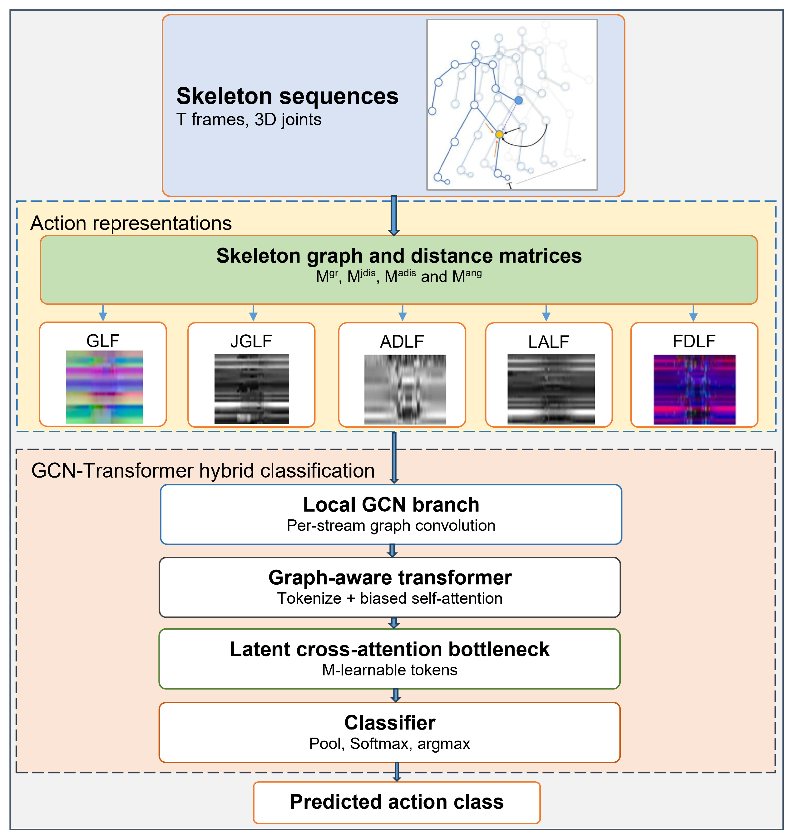
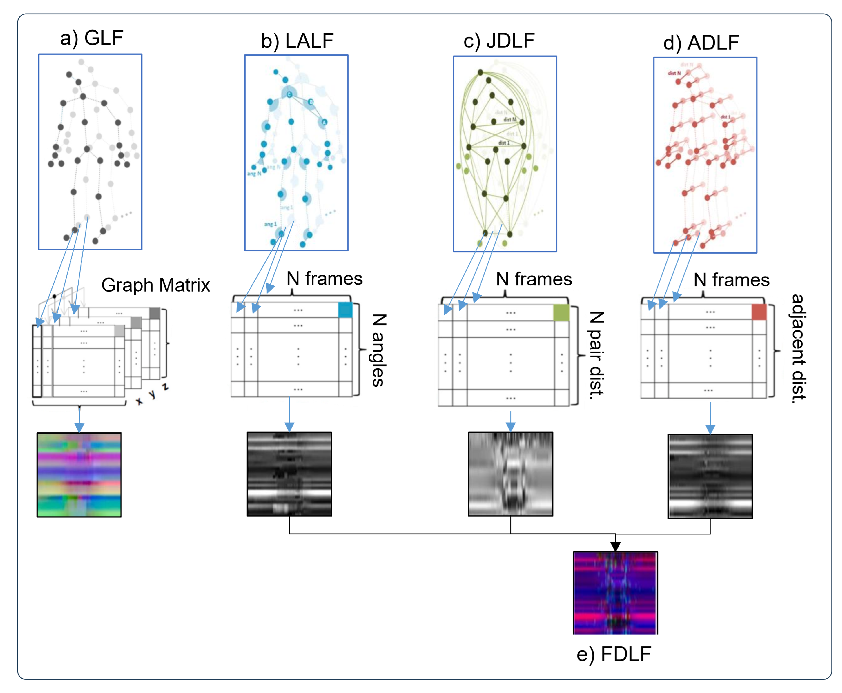
Motivated by these observations, this paper introduces HILF-GT (Hybrid Invariant Latent Feature Graph Transformer), a GCN-Transformer hybrid framework organized around several invariant spatio-temporal latent features. The representation stage characterizes each skeleton sequence from four complementary viewpoints: Graph Latent Features (GLFs) describe joint-wise structural evolution, Joint Distance Latent Features (JDLFs) encode long-range pairwise relations, Adjacent Distance Latent Features (ADLFs) capture temporal motion, and Limbs Angle Latent Features (LALFs) represent higher-order angular dynamics. Rather than following a purely image-descriptor pipeline, the proposed method keeps these latent features as structured tensors throughout learning (Figure 1). The GCN branch models local and medium-range skeleton patterns, whereas the graph-aware Transformer branch uses structural, temporal, distance, and angular biases to learn global dependencies and interactions across latent-feature streams. For long sequences, the attention cost is reduced by a latent cross-attention bottleneck, consistent with recent efficient skeleton models that emphasize kinematic priors and spatial–temporal compensation [34,35].

Although GCN-Transformer hybrids [3,4,32], graph-aware attention mechanisms [29,30,31], efficient attention bottlenecks [34,35], and multi-stream skeleton representations [23] have all been explored individually in the literature, they have rarely been brought together within a single formulation. HILF-GT’s contribution is precisely this integration, achieved by letting the invariant latent features play two roles at once. On the one hand, they serve as heterogeneous input streams, with each stream passed through a dedicated GCN branch built over its own relational structure: the physical skeleton topology for GLFs, a pair-relation graph for JDLFs, temporal edges for ADLFs, and limb-angle hyperedges for LALFs (Equation (10)). On the other hand, the same features shape the attention mechanism directly, as the joint-distance and limb-angle tensors define the learned bias terms $b_d$ and $b_a$ used in Equation (12). Whereas the existing graph Transformers derive attention bias from body topology or from fixed kinematic priors, the formulation proposed here allows the invariant descriptors to govern both the token content and the structure of the interactions among tokens. Together with a parallel two-branch design, in which stream-specific GCN embeddings are fused with the latent-bottleneck output rather than processed sequentially (Equation (13)), this coupling sets HILF-GT apart from earlier hybrid architectures. The contribution of each design choice is assessed empirically in the ablation studies reported in Section 4.4.

The main contributions of this work are as follows:

(1) We introduce spatio-temporal invariant latent-feature tensors that extend the representation beyond a single skeleton descriptor. (2) We define graph latent features to describe temporal changes in skeleton topology and joint structure. (3) We construct distance- and angle-based latent features for long-range inter-joint relations, adjacent-frame motion, and limb-angle dynamics. (4) We design a GCN-Transformer hybrid classifier that preserves local skeleton priors through graph convolution and models global cross-latent-feature dependencies through graph-aware attention with a latent bottleneck.

The rest of the paper is structured as follows: Section 2 reviews related studies on skeleton-based action recognition, Section 3 presents the proposed framework in detail, Section 4 reports the experimental results and ablation analysis, and Section 5 concludes the paper.

2. Related Work

2.1. Image-Based Skeleton Representations

Several skeleton-recognition methods begin by converting a skeleton sequence into a 2D or 3D image-like representation and then extracting features with CNNs. Wang et al. [36] proposed Joint Trajectory Maps, in which joint trajectories are projected from top, side, and front views into three images processed by separate CNN streams. Recent representation-learning studies have also explored dual spaces, local–global temporal modeling, and related tensor or image-like encodings for skeleton sequences [37,38,39]. Caetano et al. [21] selected reference joints and formed images that describe the relative positions of the remaining joints with respect to these references. These designs show that visual or map-like encodings remain useful, although they should be handled carefully when the original graph semantics are important.

Together, these studies show that structured skeleton signals can be reorganized into learnable maps while also highlighting the need for representations that retain more of the original graph structure. Rasterization is useful for visualization and for CNN-based pipelines, but it can blur the separate roles of joints, bones, temporal edges, and limb-angle relations. In the proposed methodology, the representation is, therefore, kept at the tensor level: GLFs, JDLFs, ADLFs, and LALFs remain structured graph-temporal latent features, while their image forms are used only for visualization and qualitative analysis.

2.2. GCN-Based Skeleton Action Recognition

After Graph Convolutional Networks (GCNs) became widely used for graph representation learning, Yan et al. [40] introduced ST-GCN to model spatial and temporal relations among skeleton joints. This work helped establish GCNs as a natural backbone for skeleton-based action recognition because the human body already has a graph-like structure. Shi et al. [41] developed 2s-AGCN, where the skeleton topology is learned adaptively, and joint and bone information are handled in two streams. Chen et al. [23] proposed MST-GCN with multi-scale spatial and temporal graph convolutions to capture short-range joint dependencies and longer temporal patterns. Kilis et al. [42] improved robustness through feature imputation and a clustered adjacency matrix. CTR-GCN [24] learns multiple channel-wise dynamic topologies and refines a shared topology for feature aggregation. Zhou et al. [43] also addressed ambiguous action classes using a feature-refinement head.

These methods demonstrate the strength of GCNs for local skeleton structure and medium-range spatio-temporal modeling. Nevertheless, a GCN branch alone may be insufficient for global dependencies between distant joints, long temporal intervals, or heterogeneous latent features such as distances and angles. For this reason, the proposed framework uses the GCN branch as the local skeleton expert and assigns global and cross-latent-feature reasoning to graph-aware attention.

2.3. Attention-Based Skeleton Action Recognition

Attention mechanisms have also been used extensively to improve skeleton feature learning. Si et al. [44] proposed SR-TSL, which combines spatial reasoning with temporal stack learning. In a related study, Si et al. [45] integrated GCN and LSTM modules to capture spatial structure and dynamic temporal features jointly. Pang et al. [28] introduced IGFormer for human interaction recognition, using semantic body partitions together with a Transformer-based prediction module. Bavil et al. [27] applied self-attention to model global joint dependencies and focus on action-specific joints. Nikpour and Armanfard [46] used deep reinforcement learning to remove joints with limited discriminative value.

More recent graph-aware Transformer designs indicate that attention benefits from explicit structural bias. Kinematic-enhanced hypergraph convolution, topology-adaptive hypergraph Transformer networks, and reinforced graph Transformer models all use additional structural constraints to improve skeleton reasoning [29,30,31]. These studies support the main design principle of our methodology: GCN blocks model the local body topology, whereas biased attention captures long-range frame-joint relations and interactions across latent-feature streams. Because full self-attention over all frame-joint tokens is costly for long sequences, the proposed model also includes a latent cross-attention bottleneck in line with recent efficient skeleton-recognition models that combine kinematic priors and spatial–temporal compensation [34,35].

2.4. Positioning of the Proposed Method with Respect to Prior Hybrid Architectures

Table 1. Conceptual comparison between HILF-GT and representative hybrid and graph-aware attention methods.

Method	Multi-Stream with Stream-Specific Graphs	Feature-Derived Attention Bias	Parallel GCN- Transformer Branches	Latent Bottleneck Over Cross-Stream Tokens
ST-TR [32]	–	–	–	–
IGFormer [28]	–	partial (topology)	–	–
Kinematic-HGCN [29]	–	partial (hyperedges)	–	–
THTFormer [30]	–	partial (hyperedges)	–	–
RL-GTN [31]	–	partial (topology)	–	–
2s-AGCN/MST-GCN [23,41]	partial (shared graph)	–	–	–
Kinematic-prior models [34,35]	–	partial (fixed priors)	–	partial (single stream)
HILF-GT (proposed)	√	√	√	√

outlines the conceptual differences between HILF-GT and representative GCN-Transformer and graph-aware attention methods. ST-TR [32] replaces graph convolution altogether with full spatial–temporal self-attention, which means it neither retains stream-specific graph priors nor keeps the quadratic cost of attention over all frame-joint tokens under control. IGFormer [28], the hypergraph Transformer networks [29,30], and the reinforced graph Transformer of RL-GTN [31] do introduce structural bias into attention, but this bias comes from body topology, learned hyperedges, or reinforcement-optimized topology rather than from invariant distance and angle descriptors, and each of these models still operates on a single skeleton stream.

Multi-stream GCNs [23,41] process joint, bone, and motion streams in parallel, yet all of them share the same physical skeleton graph; in contrast, the four streams of HILF-GT are each built over a distinct relational structure and interact only through biased cross-stream attention. Efficient models built on kinematic priors [34,35] reduce redundancy within a single stream, whereas the latent bottleneck in HILF-GT compresses a heterogeneous token set spanning frames, joints, and four latent-feature streams at once. To the best of our knowledge, no earlier skeleton-recognition model combines (i) invariant latent features retained as structured tensors with stream-specific relation sets, (ii) attention biases parameterized by these same invariant features, and (iii) a parallel GCN-Transformer design fused through a latent cross-attention bottleneck. The empirical contribution of each of these elements is quantified through the ablation studies in Section 4.4.

3. Methodology

As shown in Figure 1, the HILF-GT framework consists of two connected stages: invariant latent-feature construction and GCN-Transformer hybrid classification. The first stage converts the skeleton sequence into complementary graph, distance, motion, and angle latent-feature tensors. The second stage learns local skeleton patterns with GCN blocks and models global cross-latent-feature dependencies with graph-aware attention.

In Figure 1, the block labeled “Local GCN branch” denotes four stream-specific GCN branches, one for each of GLFs, JDLFs, ADLFs, and LALFs, operating in parallel and independently, each governed by its own relation set ${\mathcal{R}}_s$ and weights, as defined in Equation (10). The resulting stream embeddings ${\mathbf{H}}_{GLF}^{\left(L\right)}$, ${\mathbf{H}}_{JDLF}^{\left(L\right)}$, ${\mathbf{H}}_{ADLF}^{\left(L\right)}$, and ${\mathbf{H}}_{LALF}^{\left(L\right)}$ are concatenated and tokenized (Equation (11)) to form the input of the graph-aware Transformer branch, which applies structurally biased self-attention jointly across frame, joint, and latent-feature-stream tokens (Equation (12)) and is subsequently refined by the latent cross-attention bottleneck (Equation (13)). The GCN branch and the Transformer branch thus act as two relatively independent feature-learning experts, operating respectively on parallel per-stream inputs and on joint cross-stream tokens, rather than forming a single sequential pipeline. The classifier does not operate on the bottleneck output ${\mathbf{U}}^{\left(N_b\right)}$ alone: as shown in Equation (13), the pooled representation $\mathbf{h}$ is formed by concatenating the bottleneck output with the four per-stream GCN embeddings ${\mathbf{H}}_{GLF}^{\left(L\right)}$, ${\mathbf{H}}_{JDLF}^{\left(L\right)}$, ${\mathbf{H}}_{ADLF}^{\left(L\right)}$, and ${\mathbf{H}}_{LALF}^{\left(L\right)}$, so that local (GCN) and global (Transformer/bottleneck) representations are fused immediately before the softmax classifier of Equation (14).

3.1. Action Representation

We define the skeleton sequence as $\mathcal{S}={\left\{{\mathbf{P}}_t\right\}}_{t=1}^T$, where T is the number of frames, and ${\mathbf{P}}_t\in {\mathbb{R}}^{N\times 3}$ is the pose matrix at frame t. The skeleton topology is represented by the graph $\mathcal{G}=(\mathcal{V},\mathcal{E})$, where $\mathcal{V}={\left\{v_i\right\}}_{i=1}^N$ and $\mathcal{E}$ contains the physical skeleton bones. The coordinate of joint i on axis c in frame t is denoted by $p_{i,c}^{\left(t\right)}$, and the corresponding joint position is ${\mathbf{p}}_i^{\left(t\right)}=(p_{i,1}^{\left(t\right)},p_{i,2}^{\left(t\right)},p_{i,3}^{\left(t\right)})$, where N is the number of joints (vertices). Following De Boissiere and Noumeir [38], the skeleton sequence is normalized by using the “middle of the spine” joint in the first frame as the new coordinate-system origin.

3.1.1. Skeleton Graph Matrix

For each pose, ${\mathbf{P}}_t$, represented as an $N\times 3$ matrix, the symmetric adjacency matrix is defined as $\mathbf{A}=\{a_{i,j}\mid i,j=1,\dots ,N\}$, where $a_{i,j}=1$ when joints i and j are connected, and $a_{i,j}=0$ otherwise. The normalized adjacency matrix ${\mathbf{A}}^{\prime }$ is obtained by dividing each row by the sum of its entries. The graph-transformed pose features for frame t are then computed as

$$\begin{array}{cc}\hfill {\mathbf{Y}}_t^{gr}& = {\mathbf{P}}_t^{\top }{\mathbf{A}}^{\prime }\hfill \\ \hfill & = \left[\begin{array}{cccc}{p}_{1,1}^{\left(t\right)}& p_{2,1}^{\left(t\right)}& \dots & p_{N,1}^{\left(t\right)}\\ p_{1,2}^{\left(t\right)}& p_{2,2}^{\left(t\right)}& \dots & p_{N,2}^{\left(t\right)}\\ p_{1,3}^{\left(t\right)}& p_{2,3}^{\left(t\right)}& \dots & p_{N,3}^{\left(t\right)}\end{array}\right]\left[\begin{array}{cccc}{a}_{1,1}^{\prime }& a_{1,2}^{\prime }& \dots & a_{1,N}^{\prime }\\ a_{2,1}^{\prime }& a_{2,2}^{\prime }& \dots & a_{2,N}^{\prime }\\ ⋮& ⋮& \ddots & ⋮\\ a_{N,1}^{\prime }& a_{N,2}^{\prime }& \dots & a_{N,N}^{\prime }\end{array}\right]\hfill \\ \hfill & = \left[\begin{array}{cccc}{\tilde{p}}_{1,1}^{\left(t\right)}& {\tilde{p}}_{2,1}^{\left(t\right)}& \dots & {\tilde{p}}_{N,1}^{\left(t\right)}\\ {\tilde{p}}_{1,2}^{\left(t\right)}& {\tilde{p}}_{2,2}^{\left(t\right)}& \dots & {\tilde{p}}_{N,2}^{\left(t\right)}\\ {\tilde{p}}_{1,3}^{\left(t\right)}& {\tilde{p}}_{2,3}^{\left(t\right)}& \dots & {\tilde{p}}_{N,3}^{\left(t\right)}\end{array}\right],a_{i,j}^{\prime }={\displaystyle \frac{a_{i,j}}{{\displaystyle {\displaystyle \sum _{k=1}^N}{a}_{i,k}}}}.\hfill \end{array}$$

(1)

The superscript ⊤ denotes matrix transposition. The spatio-temporal graph representation of the sequence is expressed as the three-dimensional graph matrix ${\mathbf{X}}^{gr}\in {\mathbb{R}}^{N\times 3\times T}$:

$$\begin{array}{cc}\hfill {\mathbf{X}}^{gr}& = {\left\{{\left({\mathbf{Y}}_t^{gr}\right)}^{\top }\right\}}_{t=1}^T={\left\{{\left\{{\left\{{\tilde{p}}_{i,c}^{\left(t\right)}\right\}}_{i=1}^N\right\}}_{c=1}^3\right\}}_{t=1}^T\hfill \\ \hfill & = \left[\begin{array}{cccc}{\tilde{p}}_{1,c}^{\left(1\right)}& {\tilde{p}}_{1,c}^{\left(2\right)}& \dots & {\tilde{p}}_{1,c}^{\left(T\right)}\\ {\tilde{p}}_{2,c}^{\left(1\right)}& {\tilde{p}}_{2,c}^{\left(2\right)}& \dots & {\tilde{p}}_{2,c}^{\left(T\right)}\\ ⋮& ⋮& \ddots & ⋮\\ {\tilde{p}}_{N,c}^{\left(1\right)}& {\tilde{p}}_{N,c}^{\left(2\right)}& \dots & {\tilde{p}}_{N,c}^{\left(T\right)}\end{array}\right],c=1,2,3.\hfill \end{array}$$

(2)

Here, ${\tilde{p}}_{i,c}^{\left(t\right)}$ denotes the graph-transformed feature of joint i on coordinate axis c in frame t. The matrix ${\mathbf{X}}^{gr}$ consists of three two-dimensional matrices, one for each Cartesian axis, $c=1,2,3$, and its construction is illustrated in Figure 2a.

3.1.2. Joints Distance Matrix

Robust motion representation requires the model to capture how inter-joint distances change over time. For example, in the action “clapping,” the relative movement between the left-hand and right-hand joints is more informative than the absolute position of either hand alone. We, therefore, select $P=32$ joint pairs using the same variation criterion later formalized for limb angles in Equation (5): for each candidate pair, the mean absolute frame-to-frame change of its normalized distance ${\overline{\delta }}_i^{\left(t\right)}$ is averaged over the training split, and the P pairs with the highest scores are retained. The candidate set consists of all $\left({\displaystyle \genfrac{}{}{0pt}{}{N}{2}}\right)$ joint pairs excluding pairs directly connected by a bone, whose distance is nearly constant. The selection is performed once per dataset on the training split only and kept fixed thereafter; see Figure 2c.

For a pose, ${\mathbf{P}}_t$, let $\mathcal{P}=\{q_i\mid i=1,\dots ,P\}$ denote the selected pair set, where P is the number of pairs, and $q_i=(u_i,v_i)$ contains two joint indices. The Euclidean distance for pair $q_i$ at frame t is ${\delta }_i^{\left(t\right)}={\parallel {\mathbf{p}}_{u_i}^{\left(t\right)}-{\mathbf{p}}_{v_i}^{\left(t\right)}\parallel }_2$. To reduce the influence of body-size variation, we define ${\overline{\delta }}_i^{\left(t\right)}={\delta }_i^{\left(t\right)}/{\rho }_t$, where ${\rho }_t={\sum }_{i=1}^{N-1}{\lambda }_i^{\left(t\right)}$ is the sum of all skeleton-limb lengths ${\lambda }_i^{\left(t\right)}$ at frame t. The joint-distance matrix ${\mathbf{X}}^{jd}\in {\mathbb{R}}^{P\times T}$ is expressed as

$$\begin{array}{cc}\hfill {\mathbf{X}}^{jd}& = {\left\{{\{{\delta }_i^{\left(t\right)}/{\rho }_t\}}_{i=1}^P\right\}}_{t=1}^T={\left\{{\left\{{\overline{\delta }}_i^{\left(t\right)}\right\}}_{i=1}^P\right\}}_{t=1}^T\hfill \\ \hfill & = \left[\begin{array}{cccc}{\overline{\delta }}_1^{\left(1\right)}& {\overline{\delta }}_1^{\left(2\right)}& \dots & {\overline{\delta }}_1^{\left(T\right)}\\ {\overline{\delta }}_2^{\left(1\right)}& {\overline{\delta }}_2^{\left(2\right)}& \dots & {\overline{\delta }}_2^{\left(T\right)}\\ ⋮& ⋮& \ddots & ⋮\\ {\overline{\delta }}_P^{\left(1\right)}& {\overline{\delta }}_P^{\left(2\right)}& \dots & {\overline{\delta }}_P^{\left(T\right)}\end{array}\right].\hfill \end{array}$$

(3)

Here, ${\overline{\delta }}_i^{\left(t\right)}$ denotes the normalized distance of pair $q_i$ in pose ${\mathbf{P}}_t$.

3.1.3. Adjacent Distance Matrix

The adjacent-distance matrix measures frame-to-frame changes in joint coordinates. Given two consecutive poses, ${\mathbf{P}}_t$ and ${\mathbf{P}}_{t+1}$, the adjacent Euclidean distance of joint i is ${\Delta }_i^{\left(t\right)}={\parallel {\mathbf{p}}_i^{\left(t\right)}-{\mathbf{p}}_i^{(t+1)}\parallel }_2$, so larger values correspond to faster joint movement. The adjacent-distance matrix ${\mathbf{X}}^{ad}\in {\mathbb{R}}^{N\times (T-1)}$ is defined as

$$\begin{array}{cc}\hfill {\mathbf{X}}^{ad}& = {\left\{{\left\{{\Delta }_i^{\left(t\right)}\right\}}_{i=1}^N\right\}}_{t=1}^{T-1}={\left\{{\left\{{\parallel {\mathbf{p}}_i^{\left(t\right)}-{\mathbf{p}}_i^{(t+1)}\parallel }_2\right\}}_{i=1}^N\right\}}_{t=1}^{T-1}\hfill \\ \hfill & = \left[\begin{array}{cccc}{\parallel {\mathbf{p}}_1^{\left(1\right)}-{\mathbf{p}}_1^{\left(2\right)}\parallel }_2& {\parallel {\mathbf{p}}_1^{\left(2\right)}-{\mathbf{p}}_1^{\left(3\right)}\parallel }_2& \dots & {\parallel {\mathbf{p}}_1^{(T-1)}-{\mathbf{p}}_1^{\left(T\right)}\parallel }_2\\ {\parallel {\mathbf{p}}_2^{\left(1\right)}-{\mathbf{p}}_2^{\left(2\right)}\parallel }_2& {\parallel {\mathbf{p}}_2^{\left(2\right)}-{\mathbf{p}}_2^{\left(3\right)}\parallel }_2& \dots & {\parallel {\mathbf{p}}_2^{(T-1)}-{\mathbf{p}}_2^{\left(T\right)}\parallel }_2\\ ⋮& ⋮& \ddots & ⋮\\ {\parallel {\mathbf{p}}_N^{\left(1\right)}-{\mathbf{p}}_N^{\left(2\right)}\parallel }_2& {\parallel {\mathbf{p}}_N^{\left(2\right)}-{\mathbf{p}}_N^{\left(3\right)}\parallel }_2& \dots & {\parallel {\mathbf{p}}_N^{(T-1)}-{\mathbf{p}}_N^{\left(T\right)}\parallel }_2\end{array}\right].\hfill \end{array}$$

(4)

The computation of ${\mathbf{X}}^{ad}$ is illustrated in Figure 2d.

3.1.4. Limbs Angle Matrix

In this work, the term “limb” refers to a skeleton bone that forms an angle with an adjacent bone. The angle between adjacent skeleton limbs provides information about relative limb motion, including directional variation that cannot be fully recovered from joint distances alone. The candidate set of angles consists of all triplets $(j_a,j_b,j_c)$ in which the bones $(j_a,j_b)$ and $(j_b,j_c)$ are adjacent in the skeleton graph $\mathcal{G}$ and share the middle joint $j_b$; for the 25-joint NTU skeleton, this yields 26 candidate angles. From this set, the $U=14$ angles with the largest temporal variation are selected. For a candidate angle, k, the variation score is defined as the mean absolute frame-to-frame change averaged over all training sequences,

$$v_k={\displaystyle \frac{1}{\left|\mathcal{T}\right|}}\sum _{m\in \mathcal{T}}{\displaystyle \frac{1}{T_m-1}}{\displaystyle \sum _{t=1}^{T_m-1}}\left|{\alpha }_k^{(t+1)}-{\alpha }_k^{\left(t\right)}\right|,$$

(5)

where $\mathcal{T}$ denotes the training split and $T_m$ the length of sequence m. The U angles with the highest scores $v_k$ are retained; they are dominated by the elbow, shoulder, knee, hip, and wrist angles, which is consistent with the observation that distal and mid-limb joints carry most action-related motion. The selection is computed once per dataset on the training split only, is kept fixed for all experiments on that dataset, and is never recomputed on evaluation data, so no information from the test split enters the descriptor design. As shown in Figure 2b, the selected angles are then tracked over time to form the limb-angle matrix. For the i-th selected angle, let $(j_a,j_b,j_c)$ denote the three joint indices, where $j_b$ is the shared middle joint. The angle ${\alpha }_i^{\left(t\right)}=\angle (j_a,j_b,j_c)$ at frame t is computed using the law of cosines:

$$\begin{array}{cc}\hfill {\left({\ell }_{ac}^{\left(t\right)}\right)}^2& = {\left({\ell }_{ab}^{\left(t\right)}\right)}^2+{\left({\ell }_{bc}^{\left(t\right)}\right)}^2-2{\ell }_{ab}^{\left(t\right)}{\ell }_{bc}^{\left(t\right)}\cos \left({\alpha }_i^{\left(t\right)}\right),\hfill \\ \hfill {\alpha }_i^{\left(t\right)}& = \arccos \left({\displaystyle \frac{{\left({\ell }_{ab}^{\left(t\right)}\right)}^2+{\left({\ell }_{bc}^{\left(t\right)}\right)}^2-{\left({\ell }_{ac}^{\left(t\right)}\right)}^2}{2{\ell }_{ab}^{\left(t\right)}{\ell }_{bc}^{\left(t\right)}}}\right).\hfill \end{array}$$

(6)

Here, ${\ell }_{ab}^{\left(t\right)}$, ${\ell }_{bc}^{\left(t\right)}$, and ${\ell }_{ac}^{\left(t\right)}$ denote the Euclidean distances between the corresponding joints:

$${\ell }_{ab}^{\left(t\right)}={\parallel {\mathbf{p}}_{j_a}^{\left(t\right)}-{\mathbf{p}}_{j_b}^{\left(t\right)}\parallel }_2,{\ell }_{bc}^{\left(t\right)}={\parallel {\mathbf{p}}_{j_b}^{\left(t\right)}-{\mathbf{p}}_{j_c}^{\left(t\right)}\parallel }_2,{\ell }_{ac}^{\left(t\right)}={\parallel {\mathbf{p}}_{j_a}^{\left(t\right)}-{\mathbf{p}}_{j_c}^{\left(t\right)}\parallel }_2.$$

(7)

For pose ${\mathbf{P}}_t$, let U be the number of selected angles. The limb-angle matrix ${\mathbf{X}}^{ang}\in {\mathbb{R}}^{U\times T}$ is

$${\mathbf{X}}^{ang}={\left\{{\left\{{\alpha }_i^{\left(t\right)}\right\}}_{i=1}^U\right\}}_{t=1}^T=\left[\begin{array}{cccc}{\alpha }_1^{\left(1\right)}& {\alpha }_1^{\left(2\right)}& \dots & {\alpha }_1^{\left(T\right)}\\ {\alpha }_2^{\left(1\right)}& {\alpha }_2^{\left(2\right)}& \dots & {\alpha }_2^{\left(T\right)}\\ ⋮& ⋮& \ddots & ⋮\\ {\alpha }_U^{\left(1\right)}& {\alpha }_U^{\left(2\right)}& \dots & {\alpha }_U^{\left(T\right)}\end{array}\right].$$

(8)

3.1.5. Latent-Feature Tensors

In the proposed hybrid model, the latent features are not used as rasterized images during training. Their original matrices are kept as structured spatio-temporal tensors because joint, edge, angle, and temporal semantics are directly relevant to graph convolution and attention, while image versions are retained only for visualization and qualitative analysis. The latent-feature tensors are defined as

$$\begin{array}{cc}\hfill {\mathcal{X}}^{GLF}& = {\mathbf{X}}^{gr},\hfill \\ \hfill {\mathcal{X}}^{JDLF}& = {\mathbf{X}}^{jd},\hfill \\ \hfill {\mathcal{X}}^{ADLF}& = {\mathbf{X}}^{ad},\hfill \\ \hfill {\mathcal{X}}^{LALF}& = \left[\sin \left({\mathbf{X}}^{ang}\right),\cos \left({\mathbf{X}}^{ang}\right)\right],\hfill \\ \hfill {\mathcal{X}}^{FDLF}& = Stack({\mathcal{X}}^{JDLF},{\mathcal{X}}^{ADLF},{\mathcal{X}}^{LALF}).\hfill \end{array}$$

(9)

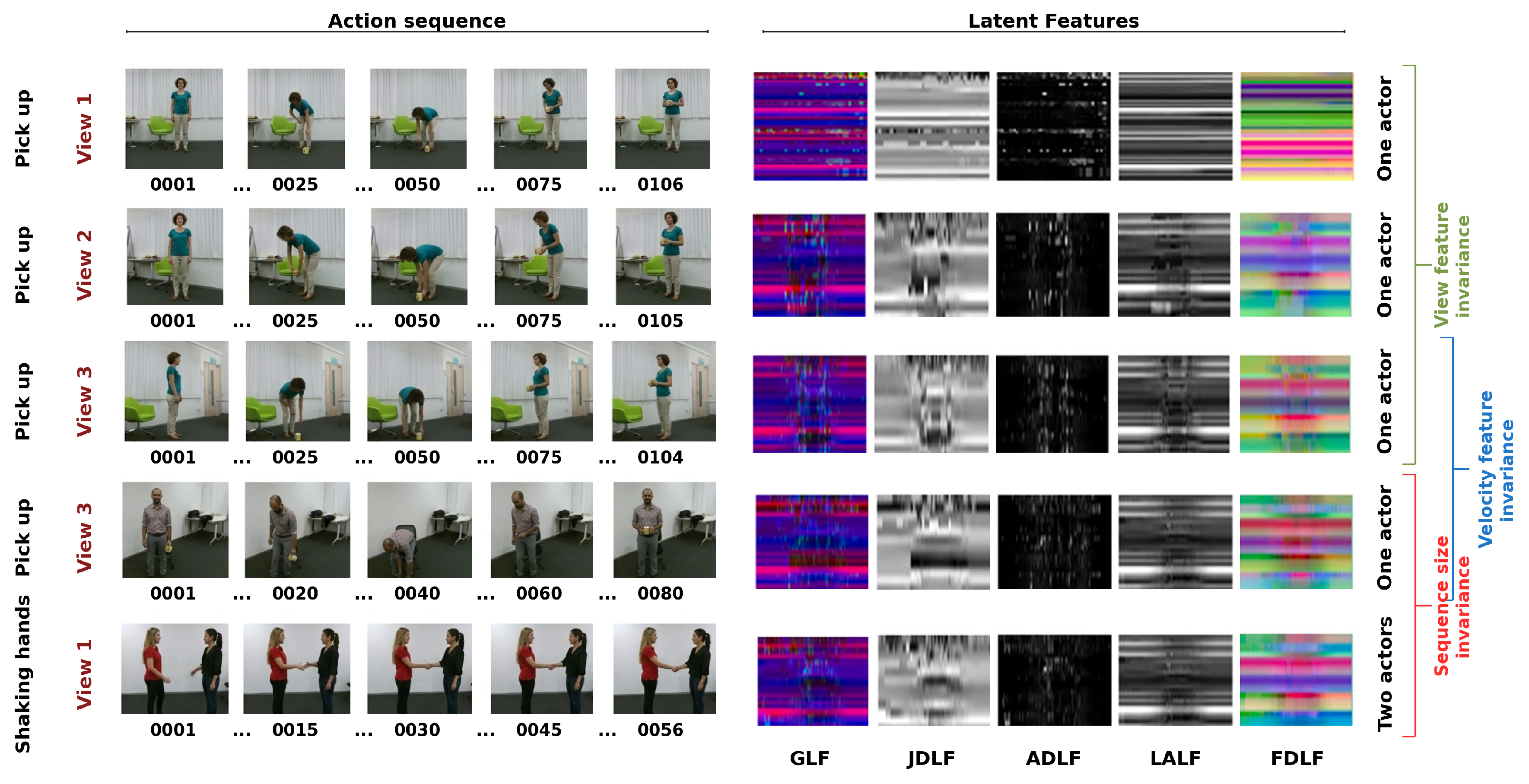
Here, ${\mathcal{X}}^{GLF}$ provides joint-wise structural information, ${\mathcal{X}}^{JDLF}$ represents long-range pairwise relations, ${\mathcal{X}}^{ADLF}$ captures temporal motion, and ${\mathcal{X}}^{LALF}$ describes higher-order angular relations. The sine–cosine encoding is used for limb angles to avoid discontinuities in raw angular values. For two-person actions such as “shaking hands,” the method doubles the number of joints N, selected pairs P, and angles U in ${\mathbf{X}}^{gr}$, ${\mathbf{X}}^{jd}$, ${\mathbf{X}}^{ad}$, and ${\mathbf{X}}^{ang}$, respectively. The formation of these matrices is illustrated in Figure 2, while Figure 3 presents their visual latent-feature forms for one-person and two-person actions.

3.2. GCN-Transformer Hybrid Action Classification

The classification model is formulated as a GCN-Transformer hybrid under the assumption that local skeleton kinematics are effectively modeled by graph convolution, while long-range dependencies among distant joints, frames, and latent-feature streams are more naturally handled by self-attention or cross-attention. The model, therefore, keeps the inductive bias of skeleton GCNs [22,40] and augments it with graph-aware attention mechanisms inspired by recent hypergraph, graph Transformer, and spatial–temporal Transformer models [29,30,31,32].

3.2.1. Local Graph Branch

Each latent-feature tensor is first projected into a shared feature dimension and then processed by a shallow spatio-temporal GCN branch. Let $s\in \mathcal{D}$ denote one latent-feature stream, where $\mathcal{D}=\{GLF,JDLF,ADLF,LALF\}$. Its initial embedding and the ℓ-th graph-convolution block are defined as

$$\begin{array}{cc}\hfill {\mathbf{H}}_s^{\left(0\right)}& = {\varphi }_s\left({\mathcal{X}}^s\right),\hfill \\ \hfill {\mathbf{H}}_s^{(\ell +1)}& = \sigma \left(\sum _{r\in {\mathcal{R}}_s}{\tilde{\mathbf{A}}}_s^{\left(r\right)}{\mathbf{H}}_s^{(\ell )}{\mathbf{W}}_s^{(\ell ,r)}\right).\hfill \end{array}$$

(10)

Here, ${\varphi }_s$ is a stream-specific linear projection, $\sigma$ is a non-linear activation, and ${\mathcal{R}}_s$ is the set of relation types used by stream s. For GLFs, ${\tilde{\mathbf{A}}}_s^{\left(r\right)}$ follows the physical skeleton topology; for JDLFs, it becomes a relation graph over the selected joint pairs; for ADLFs, it contains temporal edges between consecutive frames; and for LALFs, it is built from limb-angle hyperedges or from an equivalent line-graph projection. This branch learns local and medium-range kinematic patterns without forcing all latent-feature statistics into a single early-fusion space. The number of graph-convolution blocks, L, and the channel configuration of each branch are specified in Section 4.2.

3.2.2. Graph-Aware Attention Branch

The GCN stream outputs are converted into tokens indexed by frame and joint, and latent-feature-specific tokens are included for JDLFs, ADLFs, and LALFs:

$$\mathbf{Z}=Tokenize\left(Cat({\mathbf{H}}_{GLF}^{\left(L\right)},{\mathbf{H}}_{JDLF}^{\left(L\right)},{\mathbf{H}}_{ADLF}^{\left(L\right)},{\mathbf{H}}_{LALF}^{\left(L\right)})\right).$$

(11)

For two tokens, $i=(t_i,v_i)$ and $j=(t_j,v_j)$, attention is biased by structural, temporal, distance, and angular relations:

$$\begin{array}{cc}\hfill {\mathbf{B}}_{ij}& = b_s\left(dis{t}_{\mathcal{G}}(v_i,v_j)\right)+b_t\left(|t_i-t_j|\right)+b_d\left({\mathcal{X}}_{ij}^{JDLF}\right)+b_a\left({\mathcal{X}}_{ij}^{LALF}\right),\hfill \\ \hfill Attn\left(\mathbf{Z}\right)& = \mathrm{softmax}\left({\displaystyle \frac{\mathbf{Q}{\mathbf{K}}^{\top }}{\sqrt{d}}}+\mathbf{B}\right)\mathbf{V}.\hfill \end{array}$$

(12)

The term $dis{t}_{\mathcal{G}}(v_i,v_j)$ denotes the shortest-path distance on the skeleton graph. The learned functions $b_s$, $b_t$, $b_d$, and $b_a$ introduce graph distance, temporal offset, joint-distance, and limb-angle information into the attention bias. As a result, the Transformer branch remains aware of skeleton topology instead of applying unconstrained full attention to all frame-joint tokens.

3.2.3. Latent Cross-Attention Bottleneck

Full self-attention over all $(t,v)$ tokens has quadratic memory cost. To make the high-capacity hybrid model practical for longer sequences, we introduce a compact latent bottleneck, following the broader trend of reducing redundant spatial–temporal processing in recent skeleton-recognition models [34,35]. Let ${\mathbf{U}}^{\left(0\right)}\in {\mathbb{R}}^{R\times d}$ be R learnable latent tokens, where $R\ll TN$. The global representation is obtained by cross-attending from the latent tokens to the latent-feature tokens:

$$\begin{array}{cc}\hfill {\mathbf{U}}^{(m+1)}& = \mathrm{Transformer}\left({\mathbf{U}}^{\left(m\right)}+\mathrm{softmax}\left({\displaystyle \frac{{\mathbf{Q}}_U{\mathbf{K}}_Z^{\top }}{\sqrt{d}}}\right){\mathbf{V}}_Z\right),\hfill \\ \hfill \mathbf{h}& = Pool\left(Cat({\mathbf{U}}^{\left(N_b\right)},{\mathbf{H}}_{GLF}^{\left(L\right)},{\mathbf{H}}_{JDLF}^{\left(L\right)},{\mathbf{H}}_{ADLF}^{\left(L\right)},{\mathbf{H}}_{LALF}^{\left(L\right)})\right).\hfill \end{array}$$

(13)

Here, $N_b$ is the number of bottleneck layers. This bottleneck retains global interaction modeling and cross-latent-feature reasoning while avoiding the memory growth caused by complete self-attention over all tokens.

3.2.4. Classifier and Training Objective

The final action class is predicted from the pooled hybrid representation as follows:

$$\begin{array}{cc}\hfill \widehat{\mathbf{y}}& =\mathrm{softmax}({\mathbf{W}}_c\mathbf{h}+{\mathbf{b}}_c),\hfill \\ \hfill \widehat{c}& =\arg \underset{c}{\max }{\widehat{\mathbf{y}}}_c.\hfill \end{array}$$

(14)

The network is trained end-to-end with cross-entropy loss:

$$\mathcal{L}=-{\displaystyle \sum _{c=1}^C}{y}_c^{\ast }\log \left({\widehat{\mathbf{y}}}_c\right),$$

(15)

where C is the number of action classes, and $y_c^{\ast }$ is the one-hot ground-truth label. Under this formulation, the former late decision rule is replaced by a single differentiable model: the GCN branch provides local skeleton priors, the attention branch learns global dependencies and cross-latent-feature interactions, and the latent bottleneck controls memory cost for long action sequences.

The complete computational procedure of HILF-GT is summarized in Algorithm 1. Stage 1 is executed once per dataset on the training split and produces the fixed joint-pair set $\mathcal{P}$ and angle set $\mathcal{A}$; Stages 2 and 3 are executed for every input sequence during both training and inference. During training, the loss of Equation (15) is computed after line 18, and the parameters of all modules are updated jointly by backpropagation.

Algorithm 1 HILF-GT: latent-feature construction and hybrid classification

Require: Skeleton sequence $\mathcal{S}={\left\{{\mathbf{P}}_t\right\}}_{t=1}^T$, skeleton graph $\mathcal{G}$, trained parameters

Ensure: Predicted action class $\widehat{c}$

Stage 1: Descriptor selection (offline, once per dataset, training split only)

1: Compute variation score $v_k$ (Equation (5)) for every candidate joint pair and every candidate angle triplet   2: $\mathcal{P}\leftarrow$ top-P joint pairs;    $\mathcal{A}\leftarrow$ top-U angle triplets

Stage 2: Latent-feature construction (per sequence)

3: Normalize $\mathcal{S}$ to the spine-centered coordinate system   4: ${\mathbf{X}}^{gr}\leftarrow$ graph transform of all poses (Equations (1) and (2))   5: ${\mathbf{X}}^{jd}\leftarrow$ normalized distances of pairs in $\mathcal{P}$ (Equation (3))   6: ${\mathbf{X}}^{ad}\leftarrow$ adjacent-frame displacements (Equation (4))   7: ${\mathbf{X}}^{ang}\leftarrow$ angles of triplets in $\mathcal{A}$ (Equations (6)–(8))   8: Form tensors ${\mathcal{X}}^{GLF},{\mathcal{X}}^{JDLF},{\mathcal{X}}^{ADLF},{\mathcal{X}}^{LALF}$ (Equation (9))

Stage 3: Hybrid forward pass

9: for each stream $s\in \{GLF,JDLF,ADLF,LALF\}$ in parallel do 10:     ${\mathbf{H}}_s^{\left(0\right)}\leftarrow {\varphi }_s\left({\mathcal{X}}^s\right)$ 11:     for $\ell =0$ to $L-1$ do 12:         ${\mathbf{H}}_s^{(\ell +1)}\leftarrow \sigma \left({\sum }_{r\in {\mathcal{R}}_s}{\tilde{\mathbf{A}}}_s^{\left(r\right)}{\mathbf{H}}_s^{(\ell )}{\mathbf{W}}_s^{(\ell ,r)}\right)$              ▹ Equation (10) 13:     end for 14: end for 15: $\mathbf{Z}\leftarrow Tokenize\left(Cat({\mathbf{H}}_{GLF}^{\left(L\right)},{\mathbf{H}}_{JDLF}^{\left(L\right)},{\mathbf{H}}_{ADLF}^{\left(L\right)},{\mathbf{H}}_{LALF}^{\left(L\right)})\right)$          ▹ Equation (11) 16: $\mathbf{Z}\leftarrow Attn\left(\mathbf{Z}\right)$ with composite bias $\mathbf{B}$                ▹ Equation (12) 17: Initialize latent tokens ${\mathbf{U}}^{\left(0\right)}\in {\mathbb{R}}^{R\times d}$ 18: for $m=0$ to $N_b-1$ do 19:     ${\mathbf{U}}^{(m+1)}\leftarrow \mathrm{Transformer}\left({\mathbf{U}}^{\left(m\right)}+\mathrm{CrossAttn}({\mathbf{U}}^{\left(m\right)},\mathbf{Z})\right)$         ▹ Equation (13) 20: end for 21: $\mathbf{h}\leftarrow Pool\left(Cat({\mathbf{U}}^{\left(N_b\right)},{\mathbf{H}}_{GLF}^{\left(L\right)},{\mathbf{H}}_{JDLF}^{\left(L\right)},{\mathbf{H}}_{ADLF}^{\left(L\right)},{\mathbf{H}}_{LALF}^{\left(L\right)})\right)$         ▹ Equation (13) 22: $\widehat{\mathbf{y}}\leftarrow \mathrm{softmax}({\mathbf{W}}_c\mathbf{h}+{\mathbf{b}}_c)$;    $\widehat{c}\leftarrow \arg {\max }_c{\widehat{\mathbf{y}}}_c$               ▹ Equation (14) 23: return $\widehat{c}$

4. Experiments

4.1. Datasets

NTU-RGB+D 60 is a large-scale human action recognition dataset with 56,880 skeleton sequences from 60 action classes. For comparison with state-of-the-art methods, we follow the standard evaluation protocol of the dataset [47]: Cross-Subject (C-Sub) and Cross-View (C-View). NTU-RGB+D 120 extends NTU-RGB+D 60 by adding 60 additional action categories and contains 114,480 sequences across 120 classes. For this dataset, we use the official protocol [48]: Cross-Subject (C-Sub) and Cross-Setup (C-Set). The NW-UCLA (Northwestern-UCLA) dataset includes 1494 sequence clips from 10 actions recorded simultaneously by 3 cameras. In the benchmark setting [49], camera views 1 and 2 are used for training, while camera view 3 is used for testing. The UTD-MHAD dataset [50] contains 861 sequences from 27 actions, and its evaluation follows the Cross-Subject protocol [51].

4.2. Implementation Details

The proposed model is trained end-to-end using the latent-feature tensors defined in Section 3. Each latent-feature stream is first projected into a shared feature space and processed by the local GCN branch. The resulting stream features are then converted into frame-joint and latent-feature tokens for the graph-aware Transformer branch. We use the Adam optimizer with an initial learning rate of 0.0001, reduce the learning rate by a factor of 0.5 after the fifth epoch, and set the batch size to 32, with the cross-entropy loss in Equation (15) used as the training objective. For the ablation study, latent-feature-stream and tensor-fusion variants are also trained to evaluate the contribution of each latent feature before applying the full GCN-Transformer hybrid. The latent cross-attention bottleneck uses $R=64$ latent tokens and $N_b=2$ bottleneck layers. All experiments were implemented in PyTorch 2.5 and conducted on a machine equipped with dual Nvidia RTX 5090 GPUs, 256 GB of RAM, and an Intel Core i9-14700K CPU.

Table 2. Architecture and training configuration of HILF-GT.

Module	Setting	Value
Stream GCN branches (×4)	GCN blocks L	3
	Channel widths	64/128/256
	Activation $\sigma$/normalization	ReLU/BatchNorm
	Relation types $|{\mathcal{R}}_s|$	3 (GLFs); 2 (JDLFs, ADLFs, LALFs)
Graph-aware Transformer branch	Encoder layers	4
	Attention heads	8
	Token dimension d	256
	Feed-forward dimension	1024
Latent bottleneck	Latent tokens R	64
	Bottleneck layers $N_b$	2
	Attention heads	8
Training	Optimizer	Adam
	Initial learning rate	$1\times {10}^{-4}$ (halved after epoch 5)
	Batch size	32
	Epochs	65
	Dropout/weight decay	0.1/$1\times {10}^{-4}$
	Sequence length T	300 (NTU); 52 (NW-UCLA, UTD-MHAD)

summarizes the full architectural and training configuration of HILF-GT. Each of the four stream-specific GCN branches contains $L=3$ spatio-temporal graph convolution blocks (Equation (10)), each followed by batch normalization and a ReLU activation ($\sigma$), with channel widths of 64, 128, and 256; the stream-specific projections ${\varphi }_s$ then map each latent feature tensor into the shared feature dimension $d=256$ used throughout the subsequent modules. The relation set ${\mathcal{R}}_s$ includes three relation types for GLFs (identity, inward, and outward neighbor sets, following the spatial partitioning of [40]) and two relation types (identity and neighbor) for JDLFs, ADLFs, and LALFs. The graph-aware Transformer branch comprises 4 encoder layers with 8 attention heads, a feed-forward dimension of $4d=1024$, and the composite bias defined in Equation (12); the latent bottleneck shares the same token dimension d and head count. A dropout rate of 0.1 is applied across all attention and feed-forward sublayers, together with a weight decay of ${10}^{-4}$, and all models are trained for 65 epochs. Input sequences are temporally resampled to a fixed length of $T=300$ frames for the NTU datasets and $T=52$ frames for NW-UCLA and UTD-MHAD, using uniform sampling with random temporal offsets during training and zero-padding for shorter sequences.

4.3. Comparison with the State-of-the-Art

Table 3. Accuracy comparison between HILF-GT and state-of-the-art methods on the NTU-RGB+D 60 Cross-Subject and Cross-View benchmarks (%).

Method	C-Sub	C-View
ST-GCN [40]	81.51	88.31
SR-TSL [44]	84.82	92.42
AS-GCN [53]	86.84	94.23
2s-AGCN [41]	88.58	95.18
AGC-LSTM [45]	89.23	95.10
RA-GCN [54]	87.33	93.67
4s-Shift-GCN [55]	90.77	96.15
Dynamic-GCN [56]	91.52	96.10
MST-GCN [23]	91.75	96.63
ST-TR [32]	90.23	96.35
Ta-CNN [57]	90.37	95.24
EfficientGCN [52]	92.17	96.11
ST-SLKA [58]	90.17	96.32
Action Capsules [27]	90.10	96.34
SHARL [46]	91.14	96.24
SCA-GCN [59]	89.8	96.0
AimCLR++ [60]	80.9	85.4
SA-GCN [61]	91.5	84.7
FD-GCN [62]	90.6	96.30
ISSM [63]	81.1	86.7
DPCA-GCN [64]	88.72	94.31
HILF-GT (Proposed)	93.1	97.20

compares HILF-GT with state-of-the-art methods on the NTU-RGB+D 60 (C-Sub) and C-View benchmarks. HILF-GT achieves the highest reported accuracy under both protocols, reaching 93.1% on C-Sub and 97.20% on C-View. In particular, it improves over SHARL [46] by 1.96 percentage points on C-Sub and exceeds MST-GCN [23] by 0.57 percentage points on C-View. These gains indicate that combining invariant latent-feature tensors with local GCN processing and graph-aware attention provides a richer action representation than dynamic joint selection alone. The results on NTU-RGB+D 120, reported in

Table 4. Comparison of accuracy on NTU-RGB+D 120 for Cross-Subject and Cross-Setup benchmarks (%).

Method	C-Sub	C-Set
ST-GCN [40]	70.17	73.2
AS-GCN [53]	77.19	78.5
2s-AGCN [41]	82.25	84.2
RA-GCN [54]	81.21	82.7
4s-Shift-GCN [55]	85.39	87.6
Dynamic-GCN [56]	87.23	88.6
MST-GCN [23]	87.75	88.50
ST-TR [32]	85.71	87.10
Ta-CNN [57]	85.47	87.31
IGFormer [28]	85.44	86.52
EfficientGCN [52]	88.27	88.19
ST-SLKA [58]	86.13	87.28
AimCLR++ [60]	70.1	71.2
SA-GCN [61]	79.2	78.5
FD-GCN [62]	85.5	87.90
DPCA-GCN [64]	82.85	83.65
HILF-GT (Proposed)	88.15	90.20

, show a slightly different pattern: the method is close to the best C-Sub result, trailing EfficientGCN [52] by 0.12 percentage points, while obtaining the best C-Set accuracy at 90.20%. Compared with IGFormer [28], which uses graph representations and Transformer reasoning for human interaction recognition, HILF-GT improves by 2.71 percentage points on C-Sub and 3.68 percentage points on C-Set. This result agrees with the hybrid design, where JDLFs and LALFs provide relation-aware and higher-order angular biases for attention instead of relying only on skeleton tokens.

For the smaller NW-UCLA dataset, the results in

Table 5. Accuracy comparison on NW-UCLA for the Cross-View benchmark (%).

Method	Accuracy
AGC-LSTM [45]	93.32
VA-CNN [66]	90.27
4s-shift-GCN [55]	94.26
Ta-CNN [57]	96.21
CTR-GCN [24]	96.45
InfoGCN [65]	96.66
FRHead [43]	96.78
Action Capsules [27]	97.13
FD-GCN [62]	95.10
TSGCNeXt [67]	96.55
ACE-GCN [68]	96.6
ISSM [63]	87.9
HILF-GT (Proposed)	98.50

show that HILF-GT obtains 98.50% accuracy and outperforms FRHead [43] by 1.72 percentage points, even though FRHead includes an auxiliary feature-refinement module for ambiguous classes. It also exceeds Action Capsules [27], the next strongest method in the table, by 1.37 percentage points. This suggests that complementary latent-feature streams can help separate actions with similar global poses but different local motion or limb-angle patterns. InfoGCN [65] combines information-bottleneck learning with attention-based graph convolution; nevertheless, HILF-GT achieves higher accuracy by 1.84 percentage points, indicating that explicit invariant latent features remain useful even when strong graph-attention baselines are considered.

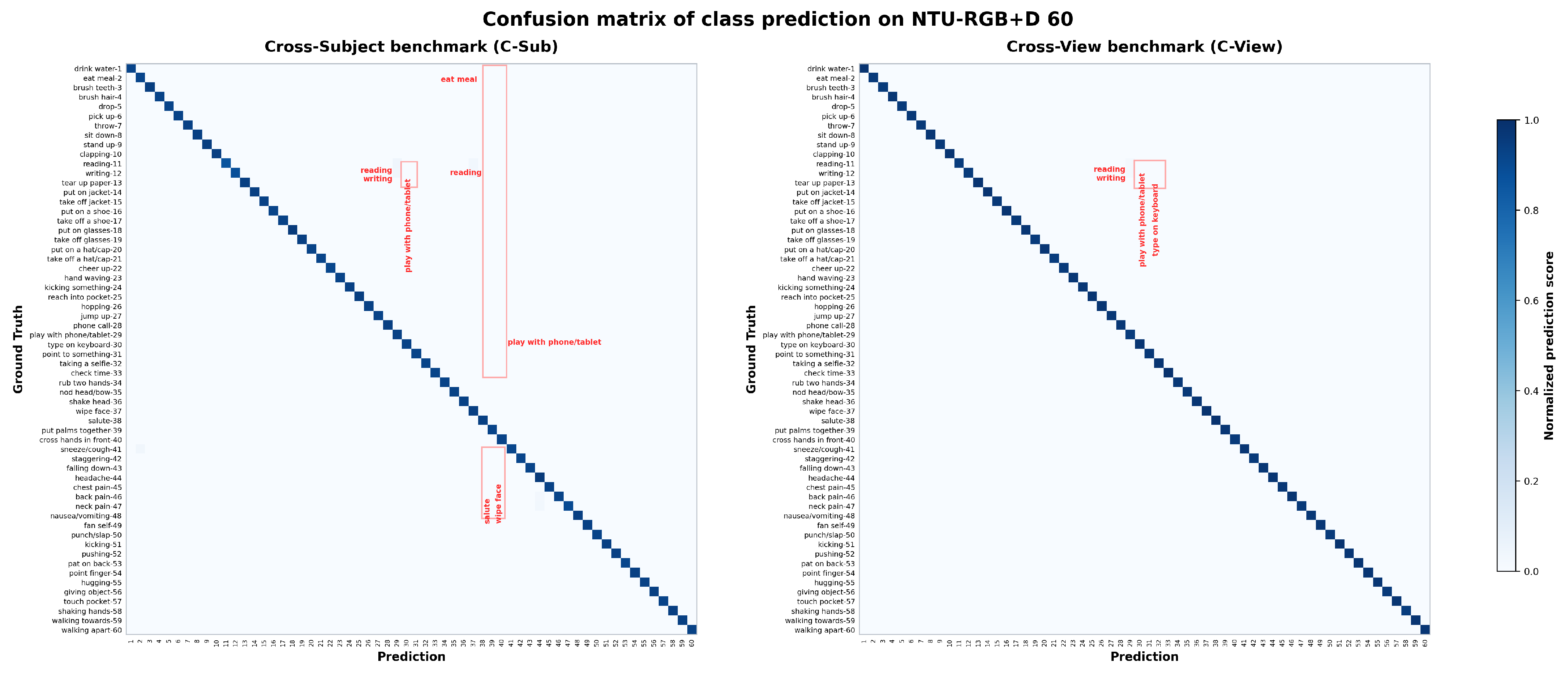
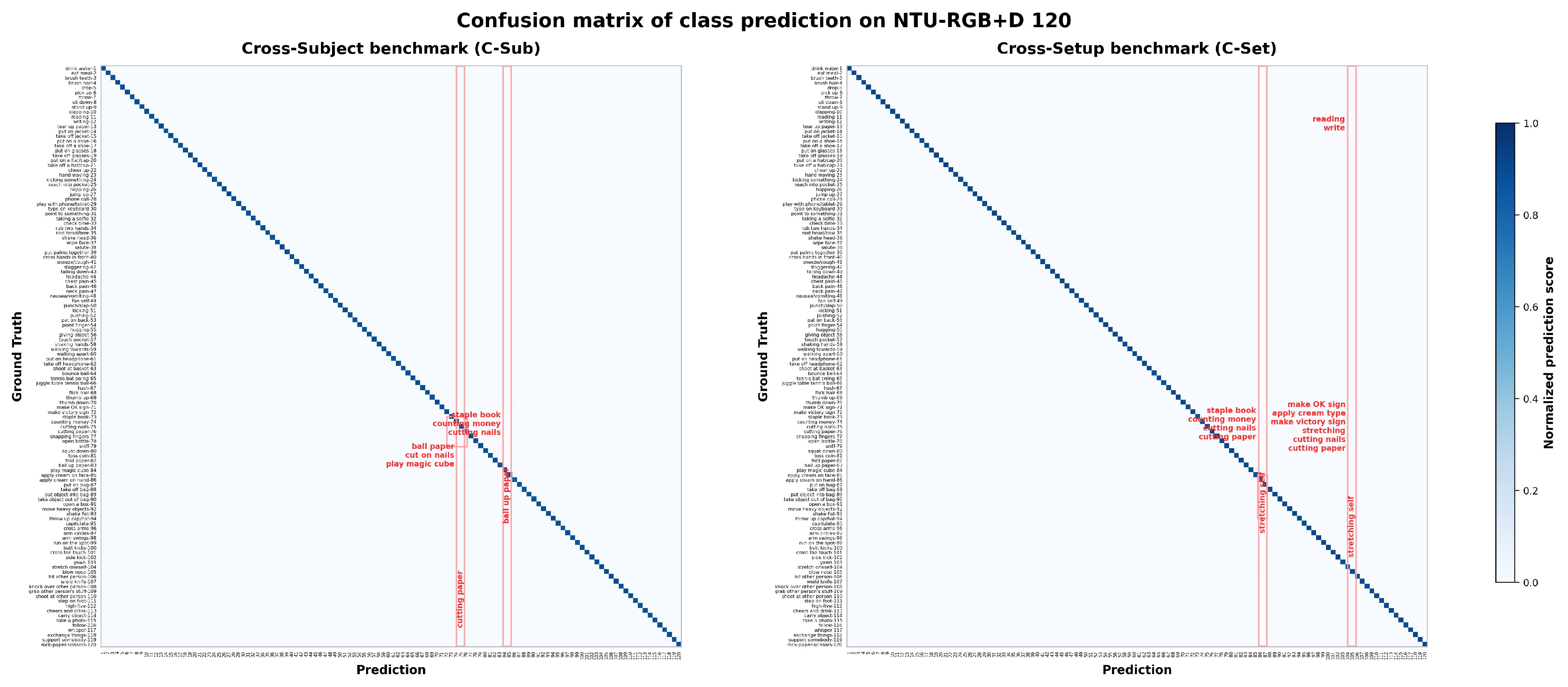
On UTD-MHAD, as shown in

Table 6. Accuracy comparison on UTD-MHAD for the Cross-Subject benchmark (%).

Method	Accuracy
Kinect [50]	66.11
Inertial [50]	67.22
Kinect&Inertial [50]	79.41
JTM [36]	85.58
Optical Spectra [69]	86.59
JDM [51]	88.41
HILF-GT (Proposed)	97.50

, HILF-GT reaches 97.50% accuracy and improves over the strongest skeleton-based baseline evaluated on this dataset, JDM [51], by 9.09 percentage points. This result supports the value of using diverse graph-, distance-, motion-, and angle-based latent features while preserving them as structured tensors.

Table 7. Descriptive summary of the accuracy of HILF-GT relative to the published results listed in Tables 3–6.

Benchmark	Methods Exceeded	$\Delta$ vs. Median	$\Delta$ vs. Best
NTU-RGB+D 60 (C-Sub)	21/21	$+3.00$	$+0.93$
NTU-RGB+D 60 (C-View)	21/21	$+1.96$	$+0.57$
NTU-RGB+D 120 (C-Sub)	15/16	$+2.73$	$-0.12$
NTU-RGB+D 120 (C-Set)	16/16	$+3.39$	$+1.60$
NW-UCLA	12/12	$+2.17$	$+1.37$
UTD-MHAD	6/6	$+15.00$	$+9.09$

summarizes the position of HILF-GT relative to the published results collected in Tables 3–6. Since these published accuracies are single-run values obtained under non-identical experimental settings, they do not constitute statistically paired observations with our results; accordingly, no formal significance test is applied to them, and the comparison is descriptive. HILF-GT exceeds every listed published result on NTU-RGB+D 60 (both protocols), NTU-RGB+D 120 (C-Set), NW-UCLA, and UTD-MHAD, and exceeds 15 of the 16 listed results on NTU-RGB+D 120 (C-Sub), where it trails EfficientGCN [52] by 0.12 percentage points. The margins are largest on NTU-RGB+D 60 (C-Sub) and NW-UCLA relative to the best published results, and on UTD-MHAD relative to the median. The statistical stability of these results under our own controlled setting is supported by the low standard deviations across independent training runs reported in Section 4.5 (at most $\pm 0.27\%$). In Figure 4 (left), the confusion matrix for the NTU-RGB+D 60 (C-Sub) benchmark shows high per-class accuracy, although visually similar actions such as ‘11-reading’ and ‘12-writing’ are sometimes confused with ‘29-play with phone/tablet’ and ‘37-salut’. Figure 4 (right) shows limited confusion in the Cross-View setting, supporting the view-invariant behavior of the latent features. On NTU-RGB+D 120, where the number of action classes increases to 120, accuracy remains stable under both Cross-Subject and Cross-Setup protocols (Figure 5), with the reported benchmark scores of 88.15% and 90.20%, respectively. Most remaining errors occur among semantically close actions, such as ‘76-cutting paper’, ‘73-stable book’, ‘74-counting money’, and ‘83-ball up paper’, or among actions with similar hand motions, such as ‘71-make OK sign’, ‘75-cutting nails’, ‘104-stretch oneself’, and ‘86-apply cream on hand’.

In quantitative terms, the largest confusions on NTU-RGB+D 60 (C-Sub) occur between ‘11-reading’ and ‘12-writing’ (1.5% of ‘reading’ samples predicted as ‘writing’), and between ‘11-reading’ and ‘29-play with phone/tablet’ (0.8%), while all remaining off-diagonal entries stay below 0.5%. In addition, in Figure 4 and Figure 5, the confusion matrixes of class prediction on NTU-RGB+D 60 and NTU-RGB+D 120 for the Cross-Subject benchmark (left) and Cross-View benchmark (right), where diagonal entries with darker blue indicate a higher proportion of samples and red-highlighted areas indicate actions that are misclassified as other classes. Owing to the matrixes size (60 × 60) and (120 × 120), per-cell numeric values are omitted for legibility; the misclassification rates of the most confused class pairs are reported in the text.

4.4. Ablation Study

4.4.1. Effect of Each Component on the Prediction

Each latent-feature stream represents a different aspect of the action: GLF models structural skeleton evolution, JDLFs capture long-range pairwise relations, ADLFs represent temporal motion, and LALFs describe angular dynamics. For simple actions, one latent-feature stream may be sufficient, whereas more complex or ambiguous actions benefit from combining latent-feature streams and allowing graph-aware attention to learn dependencies among them.

Table 8. Accuracy of latent-feature-stream variants, tensor-fusion variant, and full GCN-Transformer hybrid on different datasets (%).

Model	NTU-RGB+D 60 (C-Sub)	NTU-RGB+D 60 (C-View)	NTU-RGB+D 120 (C-Sub)	NTU-RGB+D 120 (C-Set)	NW-UCLA
GLFs	80.23	86.42	72.30	74.38	83.28
JDLFs	77.28	86.24	68.20	70.38	91.60
ADLFs	73.16	80.51	62.72	65.62	88.71
LALFs	73.41	77.19	61.24	63.27	87.27
FDLFs	81.51	85.77	72.51	74.64	92.81
tensor-fusion	87.22	91.22	76.57	90.32	95.50
full hybrid	93.10	97.20	88.15	90.20	98.50

shows that the full hybrid reaches 93.10%, 97.20%, 88.15%, 90.20%, and 98.50% on NTU-RGB+D 60 (C-Sub), NTU-RGB+D 60 (C-View), NTU-RGB+D 120 (C-Sub), NTU-RGB+D 120 (C-Set), and NW-UCLA, respectively. It outperforms all single-stream variants and exceeds the tensor-fusion configuration on four of the five benchmarks; the exception is NTU-RGB+D 120 (C-Set), where tensor fusion obtains 90.32% compared with 90.20% for the full hybrid, although the full hybrid achieves higher overall accuracy on the remaining benchmarks.

Table 9. Ablation study of latent-feature streams and hybrid fusion on NTU-RGB+D 60 (C-Sub) (%), where a check mark denotes an included component.

GLFs	JDLFs	ADLFs	LALFs	FDLFs	Hybrid	Accuracy
		√	√	√	√	88.21
√	√			√	√	89.64
√	√	√	√			88.16
	√	√	√	√	√	90.46
√		√	√	√	√	91.17
√	√		√	√	√	91.22
√	√	√		√	√	91.27
√	√	√	√		√	91.28
√	√	√	√	√		90.14
√	√	√	√	√	√	93.1

further shows that the complete component set gives the highest NTU-RGB+D 60 (C-Sub) accuracy, 93.1%, among the tested ablations.

4.4.2. Latent-Feature Tensors Versus Image-Based Transformer Classification

Table 10. Comparison between latent-feature-stream variants and MaxVIT image-based classification on NTU-RGB+D 60 (C-Sub) and NW-UCLA (%).

Latent Feature	Ours NTU60	MaxVIT NTU60	Ours NW-UCLA	MaxVIT NW-UCLA
GLFs	80.23	74.34	83.28	73.61
JDLFs	77.28	60.31	91.60	87.23
ADLFs	73.16	68.62	88.71	78.73
LALFs	73.41	64.16	87.27	82.51
FDLFs	81.51	71.65	92.81	88.35

compares the latent-feature-stream variants with MaxVIT [70,71], a state-of-the-art image Transformer applied to the visual forms of the latent features, and shows that the proposed stream variants consistently outperform direct MaxVIT classification of rasterized latent-feature images. The largest NTU-RGB+D 60 gap appears for JDLFs, where the proposed stream reaches 77.28% compared with 60.31% for MaxVIT, while the largest NW-UCLA gap appears for GLFs, with 83.28% versus 73.61%. This result supports the design choice of the proposed methodology: latent features should retain their graph, temporal, distance, and angular semantics during learning rather than being treated only as generic images. Therefore, Transformer reasoning is useful when it is graph-aware and latent-feature-aware, whereas a direct vision-Transformer classification of latent-feature images does not sufficiently exploit the underlying skeleton structure.

4.4.3. View Invariance

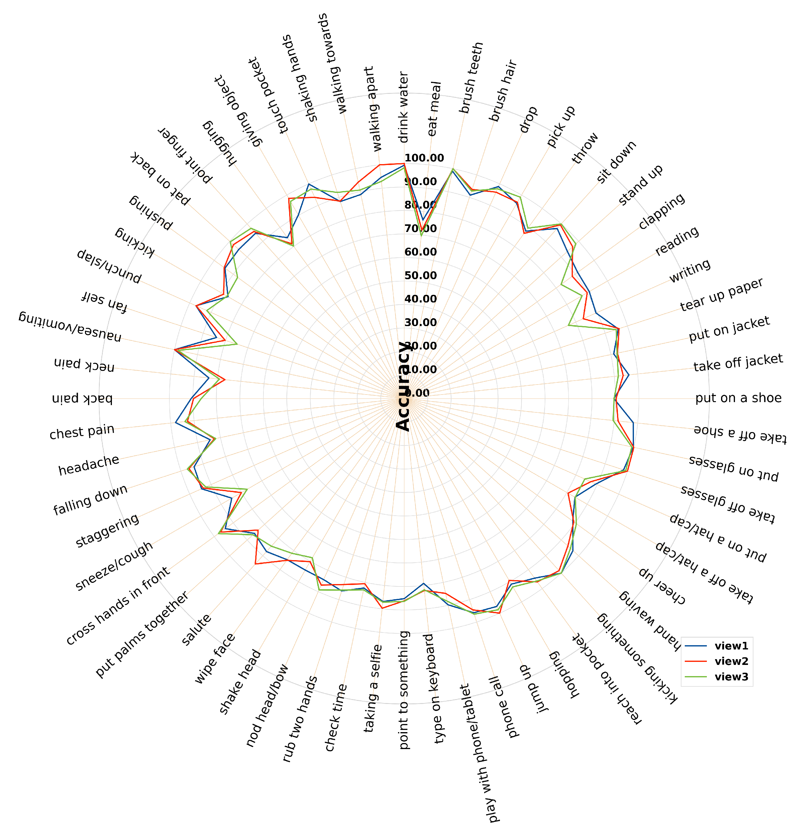
The JDLF, ADLF, and LALF streams are based on distances or angles, making them less dependent on absolute skeleton coordinates. For example, the same action observed from different camera viewpoints may produce different joint coordinates, while distances and angles between body parts remain more stable. GLFs also contribute to view robustness because it describes changes in skeleton topology rather than raw coordinates alone. Figure 4 illustrates view-invariant behavior for the ‘pick up’ action captured from three camera views in NTU-RGB+D 60. The visual latent-feature forms remain similar across views, with only minor ADLF differences caused by speed variation between adjacent frames. In the quantitative evaluation, Figure 6 reports class-level accuracy across the three views in the C-Sub benchmark, and the accuracy values for each action remain closely aligned across views, indicating that prediction depends more on the action pattern than on the camera viewpoint.

4.4.4. Velocity and Sequence Size Invariance

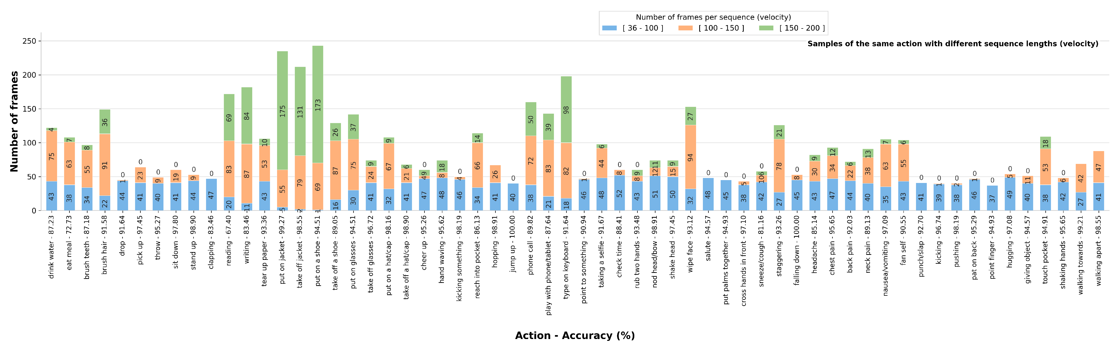
To examine latent-feature behavior under different action speeds, Figure 7 reports the accuracy of each action after grouping samples by sequence length. For this analysis, the video samples are divided into three frame intervals: [36, 100], [100, 150], and [150, 200]. For a given action, faster execution usually produces fewer frames, while slower execution produces more frames. The results show that accuracy is not strongly determined by the number of frames. For example, ‘wipe face’ reaches 93.12% accuracy across three frame ranges, whereas ‘clapping’ obtains 83.46% even though it appears in one range. Similarly, ‘put on a shoe’ remains accurate (94.51%) despite having samples in different frame ranges. This behavior can mainly be explained by two factors: ADLFs explicitly encode adjacent-frame motion, and the Transformer branch uses temporal bias and latent cross-attention to model long-range temporal dependencies without relying only on a fixed-length image representation.

4.4.5. Hyperparameter Sensitivity

To further confirm the stability of the proposed method, we examine how sensitive the hybrid architecture is to its key hyperparameters on the NW-UCLA dataset, which allows repeated training runs at a moderate computational cost.

Table 11. Hyperparameter sensitivity of HILF-GT on NW-UCLA (%). One hyperparameter is varied at a time while the others are kept at their default values (marked with *).

Hyperparameter	Value	Accuracy
Latent tokens R	32	97.20
	64 *	98.50
	128	98.05
Bottleneck layers $N_b$	1	98.25
	2 *	98.50
	3	98.31
Learning rate	$5\times {10}^{-5}$	98.02
	$1\times {10}^{-4}$ *	98.50
	$2\times {10}^{-4}$	98.38
Selected angles U	10	97.85
	14 *	98.50
	18	98.42

reports the accuracy obtained as the number of latent bottleneck tokens R, the number of bottleneck layers $N_b$, and the initial learning rate are varied around their default values, with all other settings held fixed as described in Section 4.2. Accuracy stays within a narrow range of 1.4 percentage points across all tested configurations, and none of the settings leads to training instability or divergence. Lowering R moderately reduces accuracy, consistent with the role of the latent tokens in aggregating global cross-latent-feature context, while raising R or $N_b$ beyond the default values brings no meaningful further gain and only adds a computational cost. The learning rate shows the expected mild sensitivity, with the default value of ${10}^{-4}$ giving the best balance.

We also varied the number of selected limb angles, U: reducing U to 10 lowers accuracy by 0.65 percentage points, since some discriminative angular motion is lost, whereas increasing U to 18 adds near-constant angles that contribute little additional information. Accuracy stays within one percentage point across this range, indicating that the selection is not sensitive to the exact value of U.

Combined with the low standard deviation across random seeds reported in Section 4.5 (at most $\pm 0.27\%$), these results show that the performance of HILF-GT does not rely on a finely tuned hyperparameter configuration.

4.4.6. Robustness to Skeleton Degradations

Since the proposed representation rests on invariant latent features, we also evaluate its behavior under corrupted input quantitatively. Five controlled perturbation families are applied to the NTU-RGB+D 60 Cross-Subject test set at three severity levels each, with the trained full-hybrid model kept fixed throughout; no retraining or corruption-aware augmentation is used, and all results are averaged over three random corruption seeds. The perturbations are: (i) missing joints, where a fraction of joints is independently set to zero in each frame; (ii) additive zero-mean Gaussian noise applied to all joint coordinates, with standard deviation $\sigma$ expressed in normalized coordinate units, serving as a controlled proxy for the joint-localization error typical of pose-estimation pipelines; (iii) body-part occlusion, where all joints of a selected part are removed for the entire sequence, following the protocol of RA-GCN [54]; (iv) temporal occlusion, where contiguous blocks of frames are zeroed; and (v) viewpoint perturbation, where all skeletons are rotated about the vertical axis by a random angle drawn from a symmetric interval.

Table 12. Robustness of the full HILF-GT model on NTU-RGB+D 60 (C-Sub) under controlled test-time degradations (%). Perturbations are applied to the test set only; results are averaged over three corruption seeds. The clean-test accuracy is 93.10%.

Perturbation	Severity	Accuracy	$\Delta$ vs. Clean
Missing joints	10%	91.85	$-1.25$
	20%	89.94	$-3.16$
	30%	87.41	$-5.69$
Gaussian noise	$\sigma =0.01$	92.71	$-0.39$
	$\sigma =0.03$	91.66	$-1.44$
	$\sigma =0.05$	90.38	$-2.72$
Part occlusion [54]	one arm	90.52	$-2.58$
	both legs	89.87	$-3.23$
	trunk	86.73	$-6.37$
Temporal occlusion	10% frames	92.34	$-0.76$
	20% frames	91.08	$-2.02$
	30% frames	89.25	$-3.85$
Viewpoint rotation	$\pm {15}^{\circ }$	92.94	$-0.16$
	$\pm {30}^{\circ }$	92.61	$-0.49$
	$\pm {45}^{\circ }$	92.18	$-0.92$

reports the results. The model degrades gracefully under every perturbation family. Viewpoint rotation causes the smallest accuracy loss (0.9 percentage points at $\pm {45}^{\circ }$), consistent with the design of the JDLF, ADLF, and LALF streams: inter-joint distances, frame-to-frame displacements, and limb angles are geometrically invariant to rigid rotations of the skeleton, so only the coordinate-based GLF stream is affected. Gaussian coordinate noise leads to moderate degradation (2.7 percentage points at $\sigma =0.05$), indicating tolerance to the magnitude of localization error typical of modern pose estimators. Missing joints and body-part occlusion produce the largest losses (5.7 and 6.4 percentage points at the highest severities, respectively); this outcome is expected since these corruptions directly invalidate entries of the selected joint pairs and angle triplets on which JDLFs and LALFs are built, and it points to degraded-input operation as the main robustness limitation of the descriptor-selection stage. Temporal occlusion causes intermediate degradation, mitigated by the temporal bias and the latent bottleneck, which aggregate evidence from the remaining frames. Robustness to uncontrolled pose-estimation error, including systematic differences in joint definitions, is assessed qualitatively in the transfer evaluation of Figure 9 and its accompanying discussion.

4.5. Computation Complexity

Table 13. Computation complexity comparison in parameters (M), GFLOPs and inference time (sequences/second).

Model	Parameters (M)	GFLOPs	Inference Time
ST-GCN [40]	3.1	18	47
RA-GCN [54]	5.4	34	20
2s-AGCN [41]	5.7	39	21
4s-ShiftGCN [55]	3.0	16	–
CTR-GCN [24]	0.8	8	–
DSTA-Net [72]	4.2	68	–
ST-TR [32]	15.7	252	–
HILF-GT (latent-feature stream)	0.9	9	101
HILF-GT (tensor fusion)	2.8	28	33
HILF-GT (full hybrid)	8.2	82	19

compares HILF-GT with other action recognition models in terms of GFLOPs and inference speed. The latent-feature-stream variant is the lightest HILF-GT configuration, requiring 9 GFLOPs and reaching 101 sequences/s. Tensor fusion increases computation to 28 GFLOPs and reduces inference speed to 33 sequences/s because several latent-feature tensors must be projected and processed together. The full GCN-Transformer hybrid has the highest cost among the HILF-GT variants, with 82 GFLOPs and 19 sequences/s, because it includes local GCN processing, graph-aware attention, and the latent cross-attention bottleneck. This additional computation is associated with the strongest benchmark accuracy reported for HILF-GT in Table 3, Table 4, Table 5 and Table 6. Compared with ST-TR [32], the proposed full hybrid remains substantially lighter, using 82 GFLOPs instead of 252 GFLOPs, because the latent bottleneck avoids full self-attention over all frame-joint tokens.

In addition to recognition accuracy, we further examine the proposed model with regard to its complexity and the stability of its results, as summarized in Table 13. Specifically, we report the number of trainable parameters and the computational cost (GFLOPs) of the proposed model and the compared methods, together with the mean and standard deviation of our model’s accuracy obtained over three independent training runs with different random seeds. Note that the accuracies of the compared methods are taken directly from their original publications, where only single-run results were reported; standard deviations are, therefore, not available for these methods.

For a component-level view of the computational cost,

Table 14. Component-level computational complexity of the full HILF-GT model on NTU-RGB+D 60 ($T=300$, $N=25$), measured on a single Nvidia RTX 5090 GPU. Latency is reported per sequence with batch size 1; peak GPU memory is reported for batch size 32.

Component	Params (M)	GFLOPs	Peak Memory (GB)	Latency (ms)	Throughput (seq/s)
GCN branch: GLFs	0.9	9	0.42	1.6	625
GCN branch: JDLFs	0.7	6	0.31	1.2	833
GCN branch: ADLFs	0.6	5	0.28	1.1	909
GCN branch: LALFs	0.7	6	0.30	1.2	833
Graph-aware Transformer branch	3.8	38	1.65	3.9	256
Latent cross-attention bottleneck	1.5	18	0.71	1.4	714
Full hybrid (network only)	8.2	82	3.67	10.4	96
Full hybrid (incl. latent-feature construction)	8.2	82	3.67	53.0	19

breaks the full hybrid model down into its four latent-feature stream branches and its two global modules, reporting for each component the number of trainable parameters, the computational cost in GFLOPs, the peak GPU memory usage during inference, the per-sequence latency, and the corresponding throughput. All measurements were obtained on a single Nvidia RTX 5090 GPU using NTU-RGB+D 60 sequences of $T=300$ frames; latency was measured with batch size 1 and averaged over 1000 forward passes after 100 warm-up iterations, while peak memory was recorded with the training batch size of 32. The four GCN stream branches are individually lightweight, requiring between 0.6 M and 0.9 M parameters and between 5 and 9 GFLOPs each; their costs differ according to the dimensionality of the corresponding tensors, with GLFs being the most expensive stream since it operates on the full $N\times 3\times T$ representation, whereas JDLFs, ADLFs, and LALFs operate on the reduced $P\times T$, $N\times (T-1)$, and $2U\times T$ tensors, respectively. The dominant cost comes from the graph-aware Transformer branch, which accounts for roughly 46% of the total FLOPs, while the latent cross-attention bottleneck adds a comparatively small overhead, since the number of latent tokens ($R=64$) is much smaller than the number of frame-joint tokens. Note that the construction of the latent features themselves (Equations (1)–(8)) is a parameter-free preprocessing step executed on the CPU; its cost is, therefore, excluded from Table 14 and reported separately in the latency decomposition of

Table 15. Trade-off between efficiency (seconds) and accuracy (%) on NTU-RGB+D 60 (C-Sub).

Configuration	Latent-Feature Gen.	Backbone	Hybrid Head	Total	Accuracy
full hybrid	$4.8\times {10}^{-2}$	$3.1\times {10}^{-4}$	$5.5\times {10}^{-3}$	$\approx 5.7\times {10}^{-2}$	93.10
tensor fusion	$4.6\times {10}^{-2}$	$3.1\times {10}^{-4}$	–	$\approx 4.7\times {10}^{-2}$	87.22
two latent features (FDLFs + GLFs)	$2.2\times {10}^{-2}$	$6.4\times {10}^{-5}$	$2.2\times {10}^{-3}$	$\approx 2.4\times {10}^{-2}$	88.50
single latent-feature stream (FDLFs)	${10}^{-2}$	$2.7\times {10}^{-5}$	–	$\approx {10}^{-2}$	82.22

, where it accounts for the largest share of the end-to-end runtime. In end-to-end terms, the full hybrid processes 19 sequences per second (Table 13), corresponding to an overall latency of approximately 53 ms per sequence, sufficient for near-real-time operation, given that a 300-frame sequence at 30 fps spans 10 s of video.

The latent-feature-stream configuration is fastest at 101 sequences/s, although its accuracy is considerably lower than that of the full hybrid.

4.6. Trade-Off Between Efficiency and Accuracy

Table 15 summarizes the trade-off between efficiency and accuracy, showing that latent-feature construction accounts for most of the runtime while the backbone and hybrid head add a smaller but still relevant cost; since this construction stage involves no learnable parameters and is executed on the CPU, its cost is reported here as wall-clock latency rather than in the FLOPs-based analysis of Table 14. The full hybrid obtains the highest accuracy, 93.10%, because it combines all latent-feature streams and enables cross-latent-feature attention. Tensor fusion is slightly more efficient, reducing the total time from approximately $5.7\times {10}^{-2}$ s to approximately $4.7\times {10}^{-2}$ s, but its accuracy falls to 87.22%, a decrease of 5.88 percentage points. A single latent-feature stream provides the best speed, with a total time of approximately ${10}^{-2}$ s, but the lowest accuracy, 82.22%. The two-latent-feature configuration provides an intermediate option, reaching 88.50% accuracy with an approximate total time of $2.4\times {10}^{-2}$ s. Therefore, deployment can be adapted to the target scenario: limited-action applications may use a lightweight latent-feature-stream or two-latent-feature variant, whereas accuracy-oriented applications benefit from the full GCN-Transformer hybrid.

4.7. Qualitative Evaluation

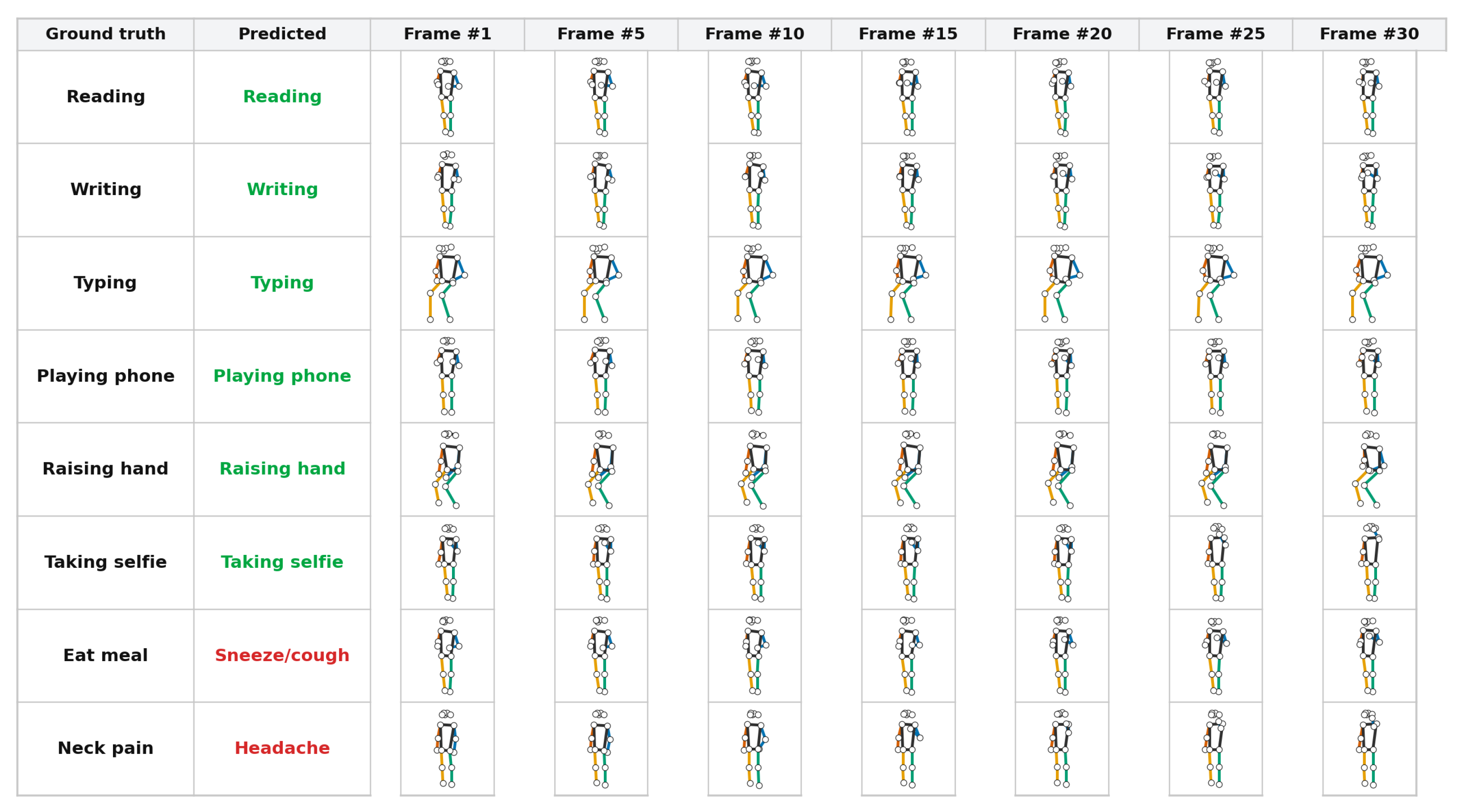
The qualitative evaluation of HILF-GT on visually similar actions is shown in Figure 8. The figure reports predictions, ground-truth labels, and key frames for test samples from NTU-RGB+D 60. The actions ‘reading’ and ‘writing’ are correctly classified despite their similar global movements because their local hand motion differs in later frames. HILF-GT also correctly recognizes similar actions such as ‘hand waving’ and ‘make a selfie’, where the distinction mainly depends on arm position and motion direction. However, the model may still fail when two actions have nearly identical skeleton motion, such as ‘neck pain’ versus ‘headache’ or ‘eat meal’ versus ‘sneeze/cough’. In such cases, skeleton data alone may not provide the object or scene context needed for full disambiguation.

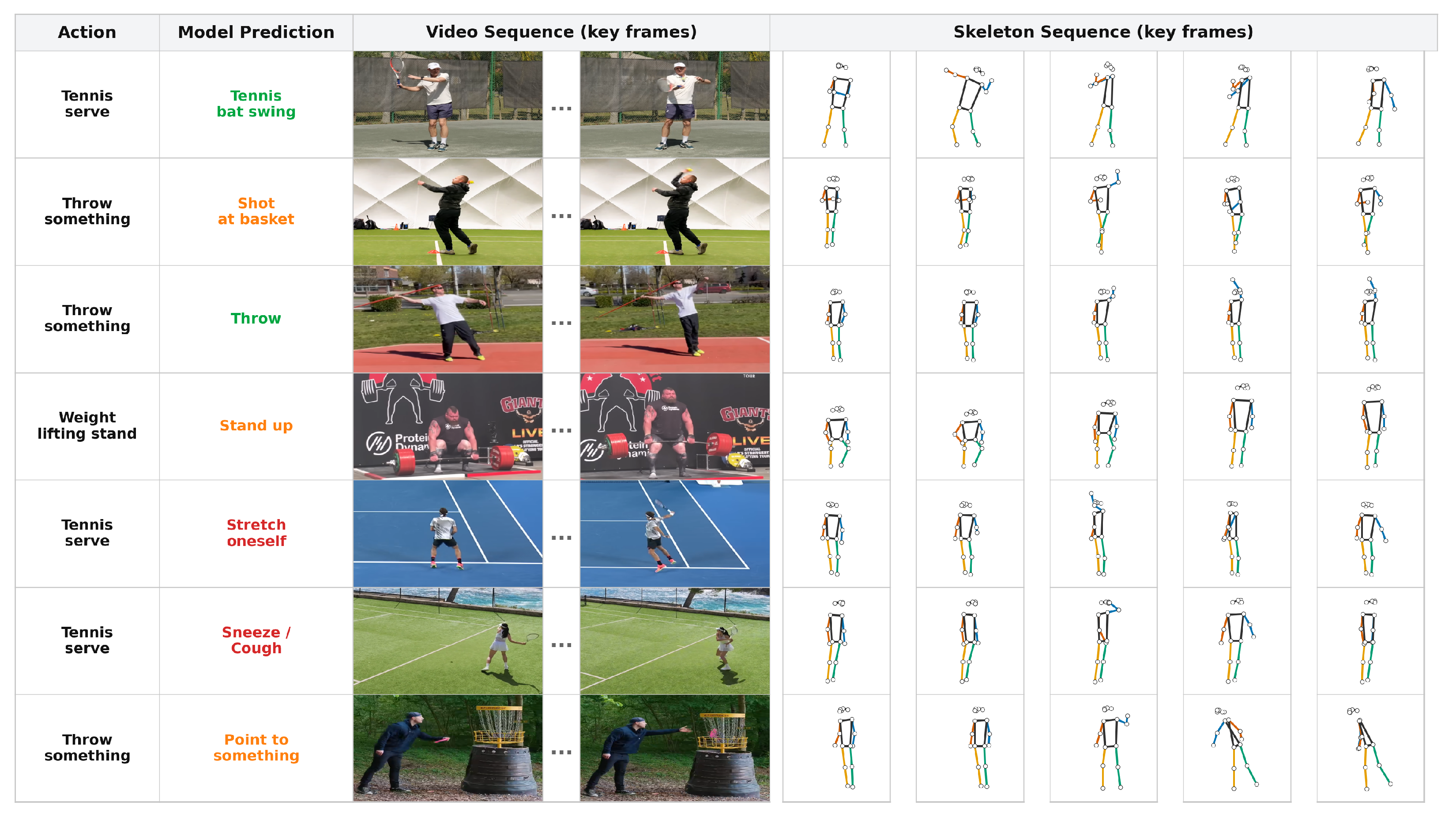
Figure 9 evaluates HILF-GT on unseen real-world videos, where the input skeleton sequences are obtained by applying a 3D pose-estimation model to RGB frames and predictions are produced by the model trained on NTU-RGB+D 120. The model generalizes well when the real action is performed in a way that resembles the training samples, as in ‘Tennis serve’ and ‘Throw something’. For partially similar motions, the prediction may be semantically close but not exact: for example, one ‘Throw something’ sample is classified as ‘Shot at basket’, and ‘Weight lifting stand’ is classified as ‘Stand up’. When the action execution differs strongly from the training distribution, misclassification becomes more likely.

The evaluation in Figure 9 should be read as a qualitative zero-shot transfer test under severe domain shift, not as a benchmark measurement of generalization. HILF-GT’s quantitative generalization ability is instead assessed through the standard evaluation protocols reported in Table 3, Table 4, Table 5 and Table 6: the cross-subject, cross-view, and cross-setup protocols measure generalization to unseen performers, camera viewpoints, and camera setups, respectively, and the consistent accuracy obtained across four datasets of different scales and sensor types (from 861 to 114,480 sequences) shows that the learned representation is not tied to a single acquisition condition. The real-world videos in Figure 9, by contrast, introduce additional domain gaps that lie outside the classifier itself: the input skeletons come from a 3D pose-estimation model rather than a Kinect sensor, which adds joint-localization noise and differences in joint definitions, and the actions are performed in unconstrained environments with execution styles that can differ substantially from the training distribution. Under these conditions, 2 of 7 clips are classified correctly and 3 further clips are assigned semantically related classes (e.g., ‘Throw something’ predicted as ‘Shot at basket’), suggesting that the model preserves the coarse semantic structure of actions even when the exact class prediction is wrong. Closing this domain gap, for instance through skeleton retargeting, pose-estimation-aware training augmentation, or lightweight fine-tuning on estimated skeletons, is left for future work.

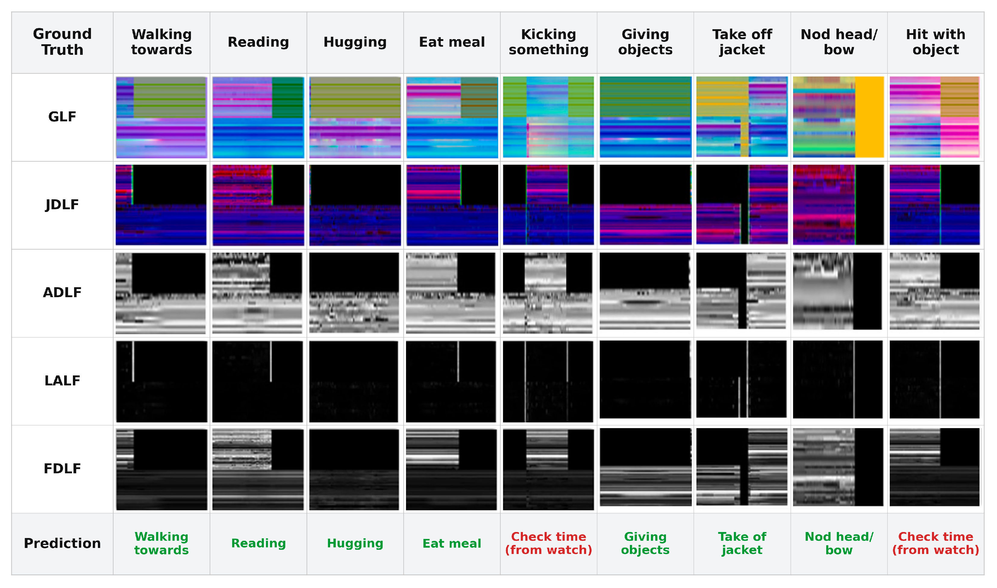
Figure 10 presents several noisy samples in which black regions indicate missing skeletons or joints. In most cases, the method still classifies the actions correctly, showing robustness even for interaction-based actions involving two individuals, such as ‘Walking towards’ and ‘Giving objects’.

4.8. Discussion

Advantages: HILF-GT obtains 93.1% and 97.20% on NTU-RGB+D 60, 88.15% and 90.20% on NTU-RGB+D 120, 98.50% on NW-UCLA, and 97.50% on UTD-MHAD, showing strong performance across datasets with different camera setups, action types, and dataset sizes. This performance is mainly due to the combination of complementary invariant latent features and a hybrid learning architecture: the latent features provide explicit graph, distance, motion, and angle information; the GCN branch preserves local skeleton priors; and the Transformer branch captures global dependencies and cross-latent-feature interactions. The ablation results in Table 8 show that replacing the full hybrid with tensor fusion reduces NTU-RGB+D 60 (C-Sub) accuracy from 93.10% to 87.22%, and Table 9 shows that removing the hybrid head reduces NTU-RGB+D 60 (C-Sub) accuracy from 93.1% to 90.14%. Together, these results confirm that the latent features are complementary rather than redundant, while the view- and velocity-invariance analyses further indicate that the model depends more on action dynamics than on camera viewpoint or sequence length. The qualitative results on similar actions (Figure 8), noisy skeletons (Figure 10), and real-world videos (Figure 9) also support the robustness of the representation.

Limitations: The main limitation of the proposed method is computational cost, because although the latent bottleneck reduces the cost of full self-attention, the complete hybrid model must still construct several latent-feature tensors and process them through both GCN and attention modules, making it slower than lightweight single-stream GCNs or latent-feature-stream variants. A second limitation is the remaining confusion between actions with very similar local and global skeleton motions, such as “eating meal” and “sneezing/coughing” (Figure 8). In these cases, skeleton data alone may not contain enough contextual information, such as the presence of food or another object.

The robustness analysis in Table 12 further shows that missing joints and body-part occlusion are the most damaging degradations, since they directly corrupt the selected joint pairs and angle triplets used by JDLFs and LALFs; making the descriptor-selection stage adaptive to incomplete skeletons is, therefore, a relevant direction for future work.

Future work: Future improvements should focus on reducing the cost of latent-feature construction and making cross-latent-feature attention more selective. One possible direction is an adaptive latent-feature-selection mechanism that activates only the most informative latent-feature streams for each input sequence. Another direction is to introduce Motion Sensitive Latent Features (MSLFs), which would emphasize the most active joints and limbs rather than representing all joints uniformly. Object-aware or RGB-assisted context could also be incorporated for actions whose skeleton motion is ambiguous without scene information.

In addition, a joint-level attention visualization that aggregates the graph-aware attention weights across heads, latent-feature streams, and the latent bottleneck will be developed to further improve the interpretability of the model.

5. Conclusions

This paper introduced HILF-GT, a Hybrid Invariant Latent Feature Graph Transformer for skeleton-based action recognition. The central design principle is that skeleton actions benefit from multiple complementary invariant latent features, including graph-structural, distance-based, motion-based, and angular descriptors, and that these features should retain their structured tensor form during learning rather than being reduced to generic images. Experiments on NTU-RGB+D 60, NTU-RGB+D 120, NW-UCLA, and UTD-MHAD show that HILF-GT achieves competitive or state-of-the-art accuracy across all four benchmarks. The ablation analysis reveals two key findings: each latent-feature stream contributes information that is not fully captured by the others, and the hybrid GCN-Transformer head accounts for a substantial portion of the overall accuracy gain over tensor-fusion and single-stream baselines. The view- and velocity-invariance results further confirm that the distance- and angle-based latent features provide robustness to viewpoint and speed variations. The main practical limitation remains the computational cost of constructing and processing multiple latent-feature streams, which future work may address through adaptive latent-feature selection or motion-sensitive feature extraction.

References

1. Li, Z.; Li, F.; Hua, G. Dynamic graph attention network for skeleton-based action recognition. Appl. Sci. 2025, 15, 4929. [Google Scholar] [CrossRef]
2. Zheng, N.; Du, Y.; Xia, H.; Liang, Z. Signal-SGN: A spiking graph convolutional network for skeleton action recognition via learning temporal-frequency dynamics. In Proceedings of the 33rd ACM International Conference on Multimedia, Dublin, Ireland, 27–31 October 2025. [Google Scholar] [CrossRef]
3. Chen, D.; Chen, M.; Wu, P.; Wu, M.; Zhang, T.; Li, C. Two-stream spatio-temporal GCN-transformer networks for skeleton-based action recognition. Sci. Rep. 2025, 15, 9482. [Google Scholar] [CrossRef] [PubMed]
4. Cui, X.; Zhang, J.; He, Y.; Wang, Z.; Zhao, W. GCN-Former: A method for action recognition using graph convolutional networks and Transformer. Appl. Sci. 2025, 15, 4511. [Google Scholar] [CrossRef]
5. Wang, J.; Sun, Y.; Tian, S. Deep learning for student behavior detection in smart classroom environments. Information 2025, 16, 949. [Google Scholar] [CrossRef]
6. Wang, H.; Weng, W.; Wang, J.; Zhao, F.; Xie, G.-S.; Geng, X.; Wang, L. Foundation model for skeleton-based human action understanding. IEEE Trans. Pattern Anal. Mach. Intell. 2026, 48, 47–61. [Google Scholar] [CrossRef] [PubMed]
7. Weng, W.; Wang, H.; Wang, J.; He, L.; Xie, G.-S. USDRL: Unified skeleton-based dense representation learning with multi-grained feature decorrelation. Proc. AAAI Conf. Artif. Intell. 2025, 39, 8332–8340. [Google Scholar] [CrossRef]
8. Wang, H.; Ma, X.; Kuang, J.; Gui, J. Heterogeneous skeleton-based action representation learning. In Proceedings of the IEEE/CVF Conference on Computer Vision and Pattern Recognition (CVPR), Nashville, TN, USA, 11–15 June 2025. [Google Scholar] [CrossRef]
9. Li, X.; Lin, J.; Li, X.; Ye, Q. Dual-geometry prior frequency nonlinear graph convolutional network for human action recognition. In Proceedings of the ICASSP 2026 IEEE International Conference on Acoustics, Speech and Signal Processing, Barcelona, Spain, 10–15 May 2026. [Google Scholar] [CrossRef]
10. Ye, Q.; Zhou, Y.; He, L.; Zhang, J.; Guo, X.; Zhang, J.; Tan, M.; Xie, W. SUGAR: Learning skeleton representation with visual-motion knowledge for action recognition. Proc. AAAI Conf. Artif. Intell. 2026, 40, 17930–17938. [Google Scholar] [CrossRef]
11. Kabulov, A.; Babadzhanov, A.; Baizhumanov, A.; Saymanov, I.; Babadjanov, A. Algorithms for solving systems of Boolean equations based on the transformation of logical expressions. Mathematics 2026, 14, 594. [Google Scholar] [CrossRef]
12. Abdusalomov, A.; Mukhiddinov, M.; Abdurashidova, K.; Kutlimuratov, A.; Marakhimov, A.; Seytnazarov, K.; Cho, Y.-I. SYMPHONIA–Enhanced multimodal emotion recognition with dual-branch dynamic attention and hierarchical adaptive fusion. Comput. Mater. Contin. 2026, 88, 077057. [Google Scholar] [CrossRef]
13. Shao, D.; Shi, M.; Liu, L. FineTec: Fine-grained action recognition under temporal corruption via skeleton decomposition and sequence completion. Proc. AAAI Conf. Artif. Intell. 2026, 40, 8842–8850. [Google Scholar] [CrossRef]
14. Patro, S.G.K.; Garg, S.; Riyazuddin, M.; Rachapudi, V.; Makharov, K.; Smerat, A.; Karimi, R. NeuroExplain-net for transparent multi-class lung cancer screening using computed tomography. Intell.-Based Med. 2026, 15, 100409. [Google Scholar] [CrossRef]
15. Murugan, J.S.; Ramkumar, M.S.; Imambi, S.S.; Sivaramkrishnan, M.; Thangavelsamy, N.; Abass, K.S.; Rakhimova, M.; Khishe, M. Gated adaptive graph causal attention decision capsule transformers network with Meerkat optimization algorithm for EEG- and EMG-guided myoelectric control in upper limb rehabilitation. Intell.-Based Med. 2026, 14, 100382. [Google Scholar] [CrossRef]
16. Liu, Y.; Yang, J.; Perera, M.; Ji, P.; Kim, D.; Xu, M.; Wang, T.; Anwar, S.; Gedeon, T.; Qin, Z. Representation-centric survey of supervised skeletal action recognition and the new benchmark. Pattern Recognit. 2026, 180, 114140. [Google Scholar] [CrossRef]
17. Zhang, J.; Lin, L.; Yang, S.; Liu, J. Self-supervised skeleton-based action representation learning: A benchmark and beyond. Int. J. Comput. Vis. 2026, 134, 38. [Google Scholar] [CrossRef]
18. Shuai, T.; Beng, S.; Khalid, F.B.; Rahmat, R.W.B.O.K. Advances in facial micro-expression detection and recognition: A comprehensive review. Information 2025, 16, 876. [Google Scholar] [CrossRef]
19. Liu, Y.; Shi, T.; Zhai, M.; Liu, J. Frequency decoupled masked auto-encoder for self-supervised skeleton-based action recognition. IEEE Signal Process. Lett. 2025, 32, 546–550. [Google Scholar] [CrossRef]
20. Wei, J.; Qin, L.; Yu, B.; Zou, T.; Yan, C.; Xiao, D.; Yu, Y.; Yang, L. VA-AR: Learning velocity-aware action representations with mixture of window attention. Proc. AAAI Conf. Artif. Intell. 2025, 39, 8286–8294. [Google Scholar] [CrossRef]
21. Caetano, C.; Brémond, F.; Schwartz, W.R. Skeleton image representation for 3D action recognition based on tree structure and reference joints. In Proceedings of the 2019 32nd SIBGRAPI Conference on Graphics, Patterns and Images (SIBGRAPI), Rio de Janeiro, Brazil, 28–31 October 2019; pp. 16–23. [Google Scholar]
22. Zhou, Y.; Xu, T.; Wu, C.; Wu, X.; Kittler, J. Adaptive hyper-graph convolution network for skeleton-based human action recognition with virtual connections. In Proceedings of the IEEE/CVF International Conference on Computer Vision (ICCV), Honolulu, HI, USA, 19–23 October 2025. [Google Scholar] [CrossRef]
23. Chen, Z.; Li, S.; Yang, B.; Li, Q.; Liu, H. Multi-scale spatial temporal graph convolutional network for skeleton-based action recognition. In Proceedings of the AAAI Conference on Artificial Intelligence, Virtual, 2–9 February 2021; pp. 1113–1122. [Google Scholar]
24. Chen, Y.; Zhang, Z.; Yuan, C.; Li, B.; Deng, Y.; Hu, W. Channel-wise topology refinement graph convolution for skeleton-based action recognition. In Proceedings of the IEEE/CVF International Conference on Computer Vision, Montreal, BC, Canada, 10–17 October 2021; pp. 13359–13368. [Google Scholar]
25. Liu, Y.; Liu, R.; Hu, Y.; Wu, M.; Xin, W.; Miao, Q.; Wu, S.; Li, L. A systematic review of skeleton-based action recognition: Methods, challenges, and future directions. IEEE Trans. Neural Netw. Learn. Syst. 2026, 37, 2046–2065. [Google Scholar] [CrossRef] [PubMed]
26. Zhu, A.; Zhu, J.; Bailey, J.; Gong, M.; Ke, Q. Semantic-guided cross-modal prompt learning for skeleton-based zero-shot action recognition. In Proceedings of the IEEE/CVF Conference on Computer Vision and Pattern Recognition (CVPR), Nashville, TN, USA, 11–15 June 2025. [Google Scholar] [CrossRef]
27. Bavil, A.F.; Damirchi, H.; Taghirad, H.D. Action capsules: Human skeleton action recognition. Comput. Vis. Image Underst. 2023, 233, 103722. [Google Scholar] [CrossRef]
28. Pang, Y.; Ke, Q.; Rahmani, H.; Bailey, J.; Liu, J. IGFormer: Interaction graph transformer for skeleton-based human interaction recognition. In Proceedings of the European Conference on Computer Vision, Tel Aviv, Israel, 23–27 October 2022; pp. 605–622. [Google Scholar]
29. Ma, N.; Sun, B.; Han, Y.; Xu, G. Kinematic enhanced hypergraph convolutional network for skeleton-based human action recognition with LLM training guides. In Proceedings of the 33rd ACM International Conference on Multimedia, Dublin, Ireland, 27–31 October 2025. [Google Scholar] [CrossRef]
30. Ma, N.; Xu, G.; Han, Y.; Sun, B. THTFormer: Topology-adaptive hypergraph Transformer network for skeleton-based action recognition. Pattern Recognit. 2026, 171, 112125. [Google Scholar] [CrossRef]
31. Korban, M.; Youngs, P.; Acton, S.T. RL-GTN: A reinforced divergence-optimized graph Transformer network for skeleton-based action recognition. Pattern Recognit. 2026, 172, 112681. [Google Scholar] [CrossRef]
32. Plizzari, C.; Cannici, M.; Matteucci, M. Skeleton-based action recognition via spatial and temporal transformer networks. Comput. Vis. Image Underst. 2021, 208, 103219. [Google Scholar] [CrossRef]
33. Filali, H.; Boulealam, C.; El Fazazy, K.; Mahraz, A.M.; Tairi, H.; Riffi, J. Meaningful multimodal emotion recognition based on capsule graph transformer architecture. Information 2025, 16, 40. [Google Scholar] [CrossRef]
34. Yang, Y.; Zhao, J.; Kuang, Z.; Ta, N.; Hong, J. Kinematic priors benefit skeleton-based action recognition. In Proceedings of the ICASSP 2026 IEEE International Conference on Acoustics, Speech and Signal Processing, Barcelona, Spain, 10–15 May 2026. [Google Scholar] [CrossRef]
35. Li, X.; Geng, Q.; Huang, Q.; Li, X.; Tang, J.; Ye, Q. Spatial-temporal self-compensating graph convolutional network for skeleton-based action recognition under data constraints. IEEE Trans. Image Process. 2026, 35, 5818–5833. [Google Scholar] [CrossRef] [PubMed]
36. Wang, P.; Li, Z.; Hou, Y.; Li, W. Action recognition based on joint trajectory maps using convolutional neural networks. In Proceedings of the 24th ACM International Conference on Multimedia, Amsterdam, The Netherlands, 15–19 October 2016; pp. 102–106. [Google Scholar]
37. Yang, Y.; Chen, H.; Liu, Z.; Hu, S.; Jiao, Y. Dual space representation learning for skeleton-based action recognition. IEEE Signal Process. Lett. 2025, 32, 2104–2108. [Google Scholar] [CrossRef]
38. Liu, R.; Chen, Y.; Gai, F.; Liu, Y.; Miao, Q.; Wu, S. Local and global spatial-temporal Transformer for skeleton-based action recognition. Neurocomputing 2025, 636, 129820. [Google Scholar] [CrossRef]
39. Alavigharahbagh, A.; Hajihashemi, V.; Machado, J.J.M.; Tavares, J.M.R.S. Deep learning approach for human action recognition using a time saliency map based on motion features considering camera movement and shot in video image sequences. Information 2023, 14, 616. [Google Scholar] [CrossRef]
40. Yan, S.; Xiong, Y.; Lin, D. Spatial temporal graph convolutional networks for skeleton-based action recognition. In Proceedings of the AAAI Conference on Artificial Intelligence, New Orleans, LA, USA, 2–7 February 2018. [Google Scholar]
41. Shi, L.; Zhang, Y.; Cheng, J.; Lu, H. Two-stream adaptive graph convolutional networks for skeleton-based action recognition. In Proceedings of the IEEE/CVF Conference on Computer Vision and Pattern Recognition, Long Beach, CA, USA, 15–20 June 2019; pp. 12026–12035. [Google Scholar]
42. Kilis, N.; Papaioannidis, C.; Mademlis, I.; Pitas, I. An efficient framework for human action recognition based on graph convolutional networks. In Proceedings of the 2022 IEEE International Conference on Image Processing (ICIP 2022), Bordeaux, France, 16–19 October 2022; pp. 1441–1445. [Google Scholar]
43. Zhou, H.; Liu, Q.; Wang, Y. Learning discriminative representations for skeleton based action recognition. In Proceedings of the IEEE/CVF Conference on Computer Vision and Pattern Recognition, Vancouver, BC, Canada, 17–24 June 2023; pp. 10608–10617. [Google Scholar]
44. Si, C.; Jing, Y.; Wang, W.; Wang, L.; Tan, T. Skeleton-based action recognition with spatial reasoning and temporal stack learning. In Proceedings of the European Conference on Computer Vision (ECCV), Munich, Germany, 8–14 September 2018; pp. 103–118. [Google Scholar]
45. Si, C.; Chen, W.; Wang, W.; Wang, L.; Tan, T. An attention enhanced graph convolutional LSTM network for skeleton-based action recognition. In Proceedings of the IEEE/CVF Conference on Computer Vision and Pattern Recognition, Long Beach, CA, USA, 15–20 June 2019; pp. 1227–1236. [Google Scholar]
46. Nikpour, B.; Armanfard, N. Spatial hard attention modeling via deep reinforcement learning for skeleton-based human activity recognition. IEEE Trans. Syst. Man Cybern. Syst. 2023, 53, 4291–4301. [Google Scholar] [CrossRef]
47. Shahroudy, A.; Liu, J.; Ng, T.T.; Wang, G. NTU RGB+D: A large scale dataset for 3D human activity analysis. In Proceedings of the IEEE Conference on Computer Vision and Pattern Recognition, Las Vegas, NV, USA, 27–30 June 2016; pp. 1010–1019. [Google Scholar]
48. Liu, J.; Shahroudy, A.; Perez, M.; Wang, G.; Duan, L.Y.; Kot, A.C. NTU RGB+D 120: A large-scale benchmark for 3D human activity understanding. IEEE Trans. Pattern Anal. Mach. Intell. 2019, 42, 2684–2701. [Google Scholar] [PubMed]
49. Wang, J.; Nie, X.; Xia, Y.; Wu, Y.; Zhu, S.C. Cross-view action modeling, learning and recognition. In Proceedings of the IEEE Conference on Computer Vision and Pattern Recognition, Columbus, OH, USA, 23–28 June 2014; pp. 2649–2656. [Google Scholar]
50. Chen, C.; Jafari, R.; Kehtarnavaz, N. UTD-MHAD: A multimodal dataset for human action recognition utilizing a depth camera and a wearable inertial sensor. In Proceedings of the 2015 IEEE International Conference on Image Processing (ICIP), Quebec City, QC, Canada, 27–30 September 2015; pp. 168–172. [Google Scholar]
51. Li, C.; Hou, Y.; Wang, P.; Li, W. Joint distance maps based action recognition with convolutional neural networks. IEEE Signal Process. Lett. 2017, 24, 624–628. [Google Scholar] [CrossRef]
52. Song, Y.F.; Zhang, Z.; Shan, C.; Wang, L. Constructing stronger and faster baselines for skeleton-based action recognition. IEEE Trans. Pattern Anal. Mach. Intell. 2022, 45, 1474–1488. [Google Scholar] [CrossRef]
53. Li, M.; Chen, S.; Chen, X.; Zhang, Y.; Wang, Y.; Tian, Q. Actional-structural graph convolutional networks for skeleton-based action recognition. In Proceedings of the IEEE/CVF Conference on Computer Vision and Pattern Recognition, Long Beach, CA, USA, 15–20 June 2019; pp. 3595–3603. [Google Scholar]
54. Song, Y.F.; Zhang, Z.; Shan, C.; Wang, L. Richly activated graph convolutional network for robust skeleton-based action recognition. IEEE Trans. Circuits Syst. Video Technol. 2020, 31, 1915–1925. [Google Scholar] [CrossRef]
55. Cheng, K.; Zhang, Y.; He, X.; Chen, W.; Cheng, J.; Lu, H. Skeleton-based action recognition with shift graph convolutional network. In Proceedings of the IEEE/CVF Conference on Computer Vision and Pattern Recognition, Seattle, WA, USA, 13–19 June 2020; pp. 183–192. [Google Scholar]
56. Ye, F.; Pu, S.; Zhong, Q.; Li, C.; Xie, D.; Tang, H. Dynamic GCN: Context-enriched topology learning for skeleton-based action recognition. In Proceedings of the 28th ACM International Conference on Multimedia, Seattle, WA, USA, 12–16 October 2020; pp. 55–63. [Google Scholar]
57. Xu, K.; Ye, F.; Zhong, Q.; Xie, D. Topology-aware convolutional neural network for efficient skeleton-based action recognition. In Proceedings of the AAAI Conference on Artificial Intelligence, Virtual, 22 February–1 March 2022; pp. 2866–2874. [Google Scholar]
58. Liu, Y.; Zhang, H.; Li, Y.; He, K.; Xu, D. Skeleton-based human action recognition via large-kernel attention graph convolutional network. IEEE Trans. Vis. Comput. Graph. 2023, 29, 2575–2585. [Google Scholar] [CrossRef] [PubMed]
59. Liu, F.; Wang, C.; Tian, Z.; Du, S.; Zeng, W. Advancing skeleton-based human behavior recognition: Multi-stream fusion spatiotemporal graph convolutional networks. Complex Intell. Syst. 2025, 11, 94. [Google Scholar]
60. Guo, T.; Liu, M.; Liu, H.; Wang, G.; Li, W. Improving self-supervised action recognition from extremely augmented skeleton sequences. Pattern Recognit. 2024, 150, 110333. [Google Scholar] [CrossRef]
61. Li, M.; Chen, K.; Bai, Y.; Pei, J. Skeleton action recognition via graph convolutional network with self-attention module. Electron. Res. Arch. 2024, 32, 2848–2864. [Google Scholar] [CrossRef]
62. Ran, R.; Yang, W. FD-GCN: Feedback directed graph convolutional network for skeleton-based action recognition. Graph. Models 2025, 142, 101306. [Google Scholar] [CrossRef]
63. Tu, Z.; Zhang, Z.; Gong, J.; Yuan, J.; Du, B. Informative Sample Selection Model for Skeleton-Based Action Recognition With Limited Training Samples. IEEE Trans. Image Process. 2025, 34, 7335–7346. [Google Scholar] [CrossRef] [PubMed]
64. Lasri, K.; El Fazazy, K.; Mohamed Mahraz, A.; Tairi, H.; Riffi, J. DPCA-GCN: Dual-Path Cross-Attention Graph Convolutional Networks for Skeleton-Based Action Recognition. Computation 2025, 13, 293. [Google Scholar] [CrossRef]
65. Chi, H.G.; Ha, M.H.; Chi, S.; Lee, S.W.; Huang, Q.; Ramani, K. InfoGCN: Representation learning for human skeleton-based action recognition. In Proceedings of the IEEE/CVF Conference on Computer Vision and Pattern Recognition, New Orleans, LA, USA, 18–24 June 2022; pp. 20186–20196. [Google Scholar]
66. Zhang, P.; Lan, C.; Xing, J.; Zeng, W.; Xue, J.; Zheng, N. View adaptive neural networks for high performance skeleton-based human action recognition. IEEE Trans. Pattern Anal. Mach. Intell. 2019, 41, 1963–1978. [Google Scholar] [CrossRef] [PubMed]
67. Liu, D.; Li, X.; Cai, Z.; Chen, P. TSGCNeXt: Dynamic-Static Multi-graph Convolution for efficient skeleton-based action recognition. Expert Syst. Appl. 2025, 276, 127081. [Google Scholar] [CrossRef]
68. Han, X.-W.; Chen, X.-Y.; Cui, Y.; Guo, Q.-Y.; Hu, W. Adaptive Channel-Enhanced Graph Convolution for Skeleton-Based Human Action Recognition. Appl. Sci. 2024, 14, 8185. [Google Scholar] [CrossRef]
69. Hou, Y.; Li, Z.; Wang, P.; Li, W. Skeleton optical spectra-based action recognition using convolutional neural networks. IEEE Trans. Circuits Syst. Video Technol. 2016, 28, 807–811. [Google Scholar] [CrossRef]
70. Tu, Z.; Talebi, H.; Zhang, H.; Yang, F.; Milanfar, P.; Bovik, A.; Li, Y. MaxViT: Multi-axis vision Transformer. In Proceedings of the European Conference on Computer Vision, Tel Aviv, Israel, 23–27 October 2022; pp. 459–479. [Google Scholar]
71. Kumar, R.; Corvisieri, G.; Fici, T.F.; Hussain, S.I.; Tegolo, D.; Valenti, C. Transfer learning for facial expression recognition. Information 2025, 16, 320. [Google Scholar] [CrossRef]
72. Shi, L.; Zhang, Y.; Cheng, J.; Lu, H. Decoupled spatial-temporal attention network for skeleton-based action-gesture recognition. In Proceedings of the Asian Conference on Computer Vision, Kyoto, Japan, 30 November–4 December 2020. [Google Scholar]
Figure 1. Overall pipeline of HILF-GT. The action representation module forms complementary spatio-temporal latent features (GLFs: Graph Latent Features, JDLFs: Joint Distance Latent Features, ADLFs: Adjacent Distance Latent Features, LALFs: Limbs Angle Latent Features, FDLFs: Fusion Distance Latent Features). In the proposed methodology, the latent-feature matrices are retained as structured tensors for learning. The classification module integrates a local GCN branch, a graph-aware Transformer branch, and a latent cross-attention bottleneck to estimate the final action class.
Information 17 00729 g001
Figure 2. Construction of complementary spatio-temporal latent features from a skeleton sequence. (a) GLFs: Graph Latent Features. (b) LALFs: Limbs Angle Latent Features. (c) JDLFs: Joint Distance Latent Features. (d) ADLFs: Adjacent Distance Latent Features. (e) FDLFs: Fusion Distance Latent Features. In the proposed hybrid model, the corresponding matrices are kept as structured tensors for learning, while their image forms are used for visualization.
Information 17 00729 g002
Figure 3. Visualization of the action representation and feature invariance under different views, velocities, sequence sizes, and numbers of actors, with key video frames shown on the left and visual forms of the latent-feature tensors used by the proposed hybrid model shown on the right.
Information 17 00729 g003
Figure 4. Confusion matrix of class prediction on NTU-RGB+D 60 for the Cross-Subject benchmark (left) and Cross-View benchmark (right), with red-highlighted areas indicating actions that are misclassified as other classes.
Information 17 00729 g004
Figure 5. Confusion matrix of class prediction on NTU-RGB+D 120 for the Cross-Subject benchmark (left) and Cross-Setup benchmark (right), with red-highlighted areas indicating actions that are misclassified as other classes.
Information 17 00729 g005
Figure 6. View-invariance analysis of HILF-GT for each class across the three NTU-RGB+D 60 camera views under the C-Sub benchmark. Overall, the prediction accuracy of each action remains closely aligned across the three views.
Information 17 00729 g006
Figure 7. Velocity–invariance analysis of HILF–GT on NTU-RGB+D 60 under the C–Sub benchmark, where each action contains video samples with different sequence lengths grouped into three categories: [36, 100], [100, 150], and [150, 200].
Information 17 00729 g007
Figure 8. Predictions and ground-truth labels for samples from the NTU-RGB+D 60 testing set, captured with settings S = 001, camera C = 001, performer P = 003, and trial R = 001. Correctly classified actions are highlighted in green, and misclassified actions are highlighted in red.
Information 17 00729 g008
Figure 9. HILF-GT predictions on unseen real-world action videos produced by the model trained on NTU-RGB+D 120, where green indicates correct predictions, red indicates incorrect predictions, orange indicates partially correct predictions, and circles mark pose similarity between the real action and the incorrect prediction.
Information 17 00729 g009
Figure 10. HILF-GT predictions on noisy samples from NTU-RGB+D 120, where black areas in the latent-feature visualizations indicate missing skeletons or joints, correct predictions are shown in green, and incorrect predictions are shown in red.
Information 17 00729 g010