An Explainability-Driven SHAP-Weighted Ensemble Framework for Fraud Detection: Insights into Model Contribution Dynamics

Abstract

Ensemble learning has been widely adopted in fraud detection; however, conventional ensemble strategies rely on uniform or performance-based weighting schemes that treat explainability as a post hoc annotation rather than an architectural component. This study addresses the research goal of whether SHAP attribution values can serve as a principled, instance-specific weighting mechanism within an ensemble, thereby embedding interpretability directly into the aggregation process. A SHAP-Weighted Ensemble (SWE) framework is proposed in which the L2 norm of each base model’s SHAP attribution vector, computed at prediction time, is used to derive instance-specific voting weights via Softmax normalization. Three linear base learners (logistic regression, robust LR, calibrated linear SVM) are combined, with LinearSHAP providing exact attribution values. A comprehensive evaluation protocol was applied on a real-world vehicle insurance claims dataset, including bootstrap 95% confidence intervals, McNemar’s test, a three-way ablation study comparing equal weighting, SWE, and validation-AUC weighting, F1-optimal threshold selection, expected calibration error, and cost-sensitive evaluation under asymmetric misclassification costs. The central finding is that SWE achieves performance statistically comparable to both simpler baselines across all evaluated metrics (ROC-AUC = 0.774, 95% CI [0.681, 0.862]; F1 = 0.679, 95% CI [0.569, 0.774]; McNemar p = 1.000), while producing a transparent, per-claim weighting trace that equal-weight voting cannot provide. A KernelSHAP influence analysis conducted directly on the SWE confirms that SHAP-derived weights are substantially aligned with actual model influence ratios (LR: 1.05×, LR_R: 1.05×, SVM: 0.81×), validating the weighting mechanism empirically. An exploratory analysis of a seven-model equal-weight diagnostic ensemble reveals a negative correlation (r = −0.721, p = 0.067) between individual model performance and ensemble influence; a theoretically coherent finding that does not reach statistical significance at conventional thresholds. The primary contribution of SWE is architectural and interpretability-driven: it produces an auditable, instance-level model-weighting mechanism grounded in SHAP attribution theory, supporting regulatory accountability under GDPR Article 22 and the EU AI Act.

1. Introduction

Vehicle insurance fraud represents a pervasive and growing threat to the global insurance industry. Annual losses attributable to fraudulent claims exceed $80 billion in developed markets alone [1], and recent studies estimate that fraud inflates premiums for honest policyholders by 15–20% [2,3]. Beyond its direct financial impact, fraudulent activity erodes actuarial integrity, distorts risk pricing, and undermines policyholder trust; systemic harms that compound over time.

Traditional rule-based detection systems, reliant on static heuristics and expert-defined thresholds, are increasingly inadequate against adaptive fraud strategies [4]. Machine learning (ML) offers a data-driven alternative capable of identifying anomalous claim patterns at scale [5,6]. However, practical deployment faces two deeply interconnected obstacles that existing literature has not systematically resolved in concert.

The first obstacle is severe class imbalance. In real-world insurance portfolios, fraudulent claims typically constitute 1–5% of all submissions [7], though the dataset employed in this study exhibits a prevalence of approximately 24.7%, a more moderate but still operationally significant imbalance. Standard ML algorithms minimize overall loss, which causes them to optimize for the majority (non-fraud) class while achieving low sensitivity to the minority (fraud) class [8]. This failure mode is operationally costly: missed fraud cases (false negatives) generate direct financial losses, while excessive false positives waste investigative resources and damage policyholder relationships.

The second obstacle is interpretability. Regulatory frameworks, including the European Union’s General Data Protection Regulation (GDPR) Article 22 and the emerging AI Act, increasingly mandate that automated decisions affecting individuals be explainable and auditable [9]. Highly performant fraud models, particularly gradient-boosted ensembles and deep neural networks, typically operate as black boxes that resist transparent interpretation, creating a fundamental tension between predictive power and regulatory compliance.

A review of the recent literature reveals that these two obstacles are generally treated as independent engineering problems. Class imbalance is commonly addressed through oversampling techniques such as the synthetic minority oversampling technique (SMOTE), undersampling, or cost-sensitive learning, while interpretability is introduced after model training through post hoc explanation methods such as SHapley Additive exPlanations (SHAP) or local interpretable model-agnostic explanations (LIME). This sequential and largely siloed approach is methodologically limited: it treats explainability as an external diagnostic layer rather than as an intrinsic component of the predictive architecture, and it fails to exploit the potential relationship between a model’s explanatory behavior and its predictive reliability.

To address the identified gap, this study introduces a SHAP-Weighted Soft Voting Ensemble (SWE); a framework in which SHapley Additive exPlanations (SHAP) values are repurposed from post hoc explanatory tools into a dynamic weighting mechanism governing each base learner’s contribution to the ensemble’s final prediction. In this architecture, instance-specific SHAP magnitudes provide a principled measure of each model’s explanatory influence for a given claim, allowing ensemble votes to be weighted according to their local explanatory coherence. This design integrates explainability directly into the ensemble aggregation process while preserving the predictive advantages of ensemble learning.

Beyond the insurance fraud context, the proposed framework contributes to the broader theory of ensemble learning by introducing an explainability-driven aggregation mechanism. Traditional ensemble methods, including bagging, boosting, and soft voting, typically assign either fixed weights or performance-based weights to base learners derived from global validation metrics. Such approaches implicitly assume that a model’s average predictive performance reliably reflects its reliability for all instances, an assumption that rarely holds in heterogeneous real-world datasets. The proposed SWE framework relaxes this assumption by introducing instance-specific ensemble weighting based on local explanatory behavior. By leveraging SHAP-derived attribution magnitudes as a proxy for each model’s local explanatory coherence, the method allows ensemble influence to adapt dynamically to the structural characteristics of each observation. In this sense, SWE can be viewed as a general explanation-guided ensemble aggregation strategy applicable to a wide range of predictive modeling tasks beyond fraud detection.

This paper makes four principal contributions. First, it formalizes a novel ensemble weighting scheme in which instance-specific voting weights are derived from the L2 norm of each base model’s SHAP value vector and normalized through a Softmax function. Second, it demonstrates through empirical evaluation that SWE achieves performance statistically comparable to equal-weight and performance-weighted ensemble baselines (McNemar p = 1.000, overlapping 95% bootstrap confidence intervals), while providing transparent, per-claim model weighting not available from standard soft voting; a distinction that directly addresses regulatory accountability requirements. Third, it provides a fully reproducible methodological blueprint including data preprocessing, base learner configuration, ensemble construction, multi-level SHAP analysis, statistical inference, threshold optimization, calibration assessment, and cost-sensitive evaluation. Fourth, it uncovers a performance–influence paradox (r = −0.721, p = 0.067) in the equal-weight diagnostic ensemble, a theoretically coherent finding consistent with ensemble diversity theory that establishes an empirical motivation for the proposed weighting mechanism.

A key conceptual distinction further motivates the present work. While certain base learners, such as logistic regression, are inherently interpretable at the feature level, interpretability at the ensemble level remains largely unexplored. In most ensemble frameworks, the aggregation mechanism itself is opaque: although each model may be individually interpretable, the relative influence of each model on the final prediction is not transparent. Consequently, the decision pathway from input features to ensemble output remains partially obscured. This study therefore employs SHAP not to explain the internal behavior of already interpretable models but to quantify and regulate each model’s contribution to the ensemble decision for a given instance. By embedding explanation into the aggregation mechanism, interpretability becomes an architectural property of the ensemble rather than a post hoc diagnostic layer.

The remainder of this paper is organized as follows. Section 2 reviews the relevant literature and identifies the key research gaps motivating this study. Section 3 details the methodology, including data preparation, model architecture, and evaluation protocol. Section 4 presents and discusses the experimental results. Section 5 concludes the paper with limitations and directions for future research.

2. Literature Review

2.1. The Scale and Adaptive Nature of Vehicle Insurance Fraud

Vehicle insurance fraud is not a static adversarial problem but an adaptive one. Its manifestations span a wide spectrum: from opportunistic claim inflation and exaggerated injury reports to professionally orchestrated staged collisions and wholly fictitious claims submitted by organized crime syndicates [3]. This heterogeneity is operationally significant since a detection system optimized for one fraud archetype is systematically vulnerable to others. Benedek et al. [3] provide the most comprehensive systematic literature review of the field to date, synthesizing over 100 studies and concluding that fraud patterns evolve in direct response to deployed detection mechanisms; a cat-and-mouse dynamic that demands adaptive, data-driven detection rather than static rule-based gatekeeping.

The financial burden of this problem is substantial and global. Aslam et al. [2], in a cross-national study drawing on insurance regulatory data from multiple markets, estimate annual losses attributable to fraudulent claims in the tens of billions of dollars, with fraud cited as the primary justification for artificial intelligence adoption across major insurance groups. Harjai et al. [1] place the United States market loss alone at over $80 billion annually. Critically, the harm is not confined to insurers: Aslam et al. [2] document a direct pass-through effect to honest policyholders, with fraud-driven premium inflation estimated at 15–20% in affected market segments. This social cost, borne by parties entirely unconnected to the fraud, elevates detection from a commercial priority to a matter of systemic fairness.

Traditional rule-based systems, which encode expert heuristics such as “flag claims where repair cost exceeds vehicle valuation by more than 20%,” cannot keep pace with this adaptive threat. Liu et al. [10] demonstrate through visual analytics that fraud patterns exhibit non-stationary temporal clustering that violates the stability assumptions underpinning rule-based systems. Njeru [4], in a comprehensive review of detection approaches in the Kenyan insurance market, shows that rule-based systems generate false positive rates exceeding 40% when confronted with novel fraud typologies introduced within a single calendar year of deployment. The consensus in the literature is therefore clear: adaptive, data-driven machine learning approaches are necessary for modern fraud detection.

2.2. The Machine Learning Paradigm: Capability and Persistent Limitations

2.2.1. The Demonstrated Value of Machine Learning

Machine learning has produced significant advances in fraud detection capability over the past two decades. Early applications of logistic regression and naive Bayes [11] demonstrated that statistical pattern recognition could outperform actuarial expert judgement when trained on historical claims data. The subsequent introduction of ensemble methods, particularly random forests and gradient-boosted trees, substantially increased predictive performance.

Dhieb et al. [12] demonstrated that XGBoost achieved recall rates exceeding 85% on a proprietary automobile insurance dataset when combined with systematic feature engineering, a result that would be unattainable using rule-based systems on the same data. Dhieb et al. [9] later extended this work to a full AI-driven insurance analytics pipeline, showing that gradient-boosted models could be integrated into production systems without degrading operational throughput.

Support vector machines have also demonstrated strong performance in insurance fraud detection. Itri et al. [13] conducted a comparative evaluation of six machine learning algorithms on an automobile insurance dataset and found that SVMs with radial basis function kernels achieved the lowest false negative rate, an operationally critical metric for fraud investigators, compared with decision trees, random forests, logistic regression, naive Bayes, and AdaBoost. More recently, Khalil et al. [8] showed that linear SVMs combined with class imbalance correction achieved competitive F1-scores even on datasets containing substantial proportions of missing values, a practical consideration given the incomplete records often present in insurance management systems.

2.2.2. The Unresolved Imbalance Problem

Despite these advances, a fundamental obstacle persists: the extreme class imbalance inherent in fraud datasets. In real-world insurance portfolios, fraudulent claims typically constitute only 1–5% of submissions [7,8]. Standard machine learning algorithms minimize a global loss function that treats all instances equally; when trained on highly imbalanced data, these algorithms naturally optimize for the majority class (non-fraud) while exhibiting poor sensitivity to the minority class (fraud).

This failure mode is widely documented. Hanafy and Ming [14], in a comprehensive evaluation of six resampling strategies across seven classifiers, showed that uncorrected models achieved overall accuracies between 94% and 97% while their fraud recall fell below 20%. Such results are statistically impressive yet operationally meaningless.

Three broad corrective strategies dominate the literature. The first involves data-level resampling techniques such as SMOTE [15], random undersampling, or hybrid approaches. Hanafy and Ming [14] show that SMOTE generally outperforms undersampling but remains highly sensitive to the dataset and classifier used. Furthermore, SMOTE introduces synthetic observations that may distort the underlying data distribution.

The second approach is algorithm-level cost-sensitive learning, where minority-class errors receive higher penalties through class weighting. Khalil et al. [8] demonstrate that class weighting can achieve performance comparable to SMOTE-based approaches while preserving the original data distribution. This finding motivates the class-weighting strategy adopted in the present study.

The third approach involves threshold optimization. Nordin et al. [16] observe that most fraud detection studies report results using the default 0.5 decision threshold without analyzing the sensitivity of results to threshold variation. This oversight conflates model calibration with fraud detection performance and complicates fair comparison between competing methods.

2.2.3. The Evaluation Problem: Accuracy as a Misleading Metric

A further methodological weakness in the literature concerns evaluation metrics. Many fraud detection studies continue to rely on overall accuracy as their primary performance indicator. Surveys of vehicle insurance fraud studies published between 2019 and 2024 indicate that approximately 75% report accuracy as their headline metric [2,3,16,17,18].

However, as demonstrated by Davis and Goadrich [19], accuracy becomes misleading in the presence of class imbalance. A classifier that predicts every claim as legitimate would achieve more than 95% accuracy in most insurance portfolios while detecting no fraud cases. Precision–recall area under the curve (PR-AUC) is therefore more appropriate because it focuses on the minority class across all thresholds [20]. Yet PR-AUC remains underreported in the literature.

This evaluation gap has practical implications. Vorobyev [21] documents cases in which models reporting over 90% accuracy achieved fraud recall below 30% when evaluated on subsequent operational data. To avoid this pitfall, the present study prioritizes PR-AUC and F1-score as primary evaluation metrics while excluding overall accuracy from comparative analysis.

2.3. The Ensemble Learning Opportunity: Underexploited in This Domain

Ensemble learning combines predictions from multiple base models to improve predictive performance and robustness [22,23,24]. The theoretical foundation, comprehensively reviewed by Sagi and Rokach [6], shows that ensembles reduce prediction variance by exploiting disagreement among diverse models. This property is particularly valuable for imbalanced classification tasks where individual models may exhibit systematic biases.

Despite this theoretical advantage, ensemble learning remains underutilized in vehicle insurance fraud detection. Most studies employ gradient-boosted algorithms such as XGBoost or LightGBM as standalone classifiers rather than as components in explicitly designed ensemble architectures. Dhieb et al. [9] exemplify this pattern by applying XGBoost as a single end-to-end model.

When ensemble architectures are applied, two strategies dominate the literature, each carrying a distinct aggregation transparency problem. Khalil et al. [8] demonstrate that stacking can outperform individual classifiers; however, stacking introduces an opacity problem at the aggregation level: the meta-learner determines model influence without providing transparent justification for why certain base models dominate specific predictions, because this influence is encoded implicitly in the meta-learner’s parameters rather than as an interpretable contribution measure. Similarly, boosting methods such as AdaBoost [25] assign instance-level reweighting through an iterative error-correction procedure in which each round’s weight update is determined by the misclassification rate of the previous round, not by any direct measure of a model’s explanatory contribution to a given prediction. Across both stacking and boosting paradigms, the tension between predictive power and aggregation transparency remains unresolved; a gap the SWE framework directly addresses by making the weighting mechanism itself an explicable, auditable component of the prediction, derived from each model’s instance-specific SHAP attribution profile rather than from opaque meta-learning or iterative reweighting.

2.4. Explainable AI in Fraud Detection: Post Hoc and Architecturally Inert

The regulatory and operational imperative for explainable AI in financial decision making has grown substantially in recent years. The EU’s General Data Protection Regulation (GDPR) Article 22 establishes a right to explanation for automated decisions affecting individuals [26], while the EU AI Act designates insurance fraud scoring as a high-risk AI application subject to mandatory transparency and auditability requirements [27]. In the US context, state insurance regulatory frameworks increasingly require that algorithmic fraud determinations be contestable by policyholders; a requirement that black-box models cannot satisfy [9].

SHAP, introduced by Lundberg and Lee [28], has become the dominant XAI method in the fraud detection literature. Grounded in cooperative game theory, SHAP values provide a theoretically principled decomposition of any model’s prediction into additive feature contributions that satisfy desirable axioms: local accuracy, missingness, and consistency. In the insurance fraud context, Debener et al. [29] demonstrate that SHAP-derived explanations improve fraud investigator acceptance of ML-generated risk scores, with investigators reporting significantly higher trust in model outputs when accompanied by feature-level explanations. Vorobyev [21] uses SHAP to identify which graph-structural features of claim networks are most predictive of fraud, producing insights that translated directly into investigative protocol improvements.

However, a critical examination of how SHAP is deployed across these studies reveals a consistent and limiting pattern: SHAP is invariably applied as a post hoc diagnostic tool. The model is fully trained and deployed, predictions are made, and SHAP values are then computed to explain those predictions after the fact. Debener et al. [29], whose work most directly engages with SHAP in an insurance context, explicitly acknowledge this limitation: “the explanations describe what the model did, not why it should be trusted to do so correctly.” For ensemble systems in particular, post hoc SHAP explanations face an additional challenge: the ensemble’s aggregation logic, which models were weighted more heavily, and why, is itself opaque and unexplained.

To the best of our knowledge, no reviewed study integrates SHAP values into the model’s predictive architecture. The gap is not merely technical but conceptual: the literature treats explainability and model aggregation as separate concerns to be addressed sequentially, when they are in fact complementary dimensions of the same design problem. A model whose explanation is architecturally consequential, where the explanation is the weighting mechanism, is qualitatively more trustworthy than one where the explanation is a postprediction annotation: in the former, the explanation cannot be selectively applied or omitted, because it is constitutive of the prediction itself.

2.5. Research Gaps and Motivation for an Explanation-Weighted Ensemble Framework

From a broader machine learning perspective, these observations reveal an important limitation in current ensemble design practice. Most ensemble frameworks determine model influence using global performance statistics such as validation accuracy or AUC. This implicitly assumes that a model performing well on average is equally reliable for all instances in the input space. In heterogeneous real-world datasets, however, models often perform unevenly across different regions of the feature space. A fixed-weight aggregation strategy may therefore overemphasize models that perform well globally but poorly on specific observations. The preceding review reveals three interacting research gaps.

Gap 1—Shallow ensemble design: The literature predominantly applies either individual classifiers or equal-weight ensembles. Purposefully designed, non-uniform weighting strategies that exploit complementarity among diverse base learners, the mechanism responsible for ensembles’ theoretical advantage, remain largely unexplored for this domain [6,8].

Gap 2—Architecturally inert explainability: SHAP is universally applied as a post hoc annotation, not as a structural component. No study uses SHAP values to govern the model’s own decision-making process. Consequently, there is no mechanism by which the model’s explanatory confidence for a specific instance influences the prediction made for that instance [28,29].

Gap 3—Misleading evaluation protocols: The persistence of overall accuracy as the headline metric obscures poor minority-class performance and makes it impossible to rigorously assess whether proposed imbalance-correction strategies genuinely improve fraud detection or merely maintain a high true negative rate [19,20].

These gaps are not merely concurrent but synergistically limiting. Shallow ensemble design (Gap 1) forecloses the complementary benefits of diverse learners and leaves the ensemble’s aggregation logic arbitrary. Architecturally inert explainability (Gap 2) means that, even when SHAP is computed, it does not contribute to (and cannot improve) the prediction. Misleading evaluation (Gap 3) means that the genuine impact of imbalance correction and ensemble improvements on fraud detection is systematically underestimated or mischaracterized. Together, they define the boundary of the current state of the art and the opportunity this study addresses.

The present study’s central proposition is that Gap 1 and Gap 2 can be resolved simultaneously through a single architectural decision: using SHAP values not as post hoc annotations but as the weighting mechanism governing each base learner’s contribution to the ensemble prediction. Under this design, a model’s explanatory confidence for a specific claim, quantified by the magnitude of its SHAP attribution vector, directly determines how much influence its prediction carries in the final ensemble output. The result is an ensemble that is simultaneously purposefully weighted (addressing Gap 1), inherently explainable without post hoc approximation (addressing Gap 2), and evaluated under a rigorous imbalance-appropriate protocol (addressing Gap 3). No existing study in the vehicle insurance fraud literature has proposed or evaluated this integrated architecture.

3. Methodology: A Framework for Explanation-Weighted Fraud Detection

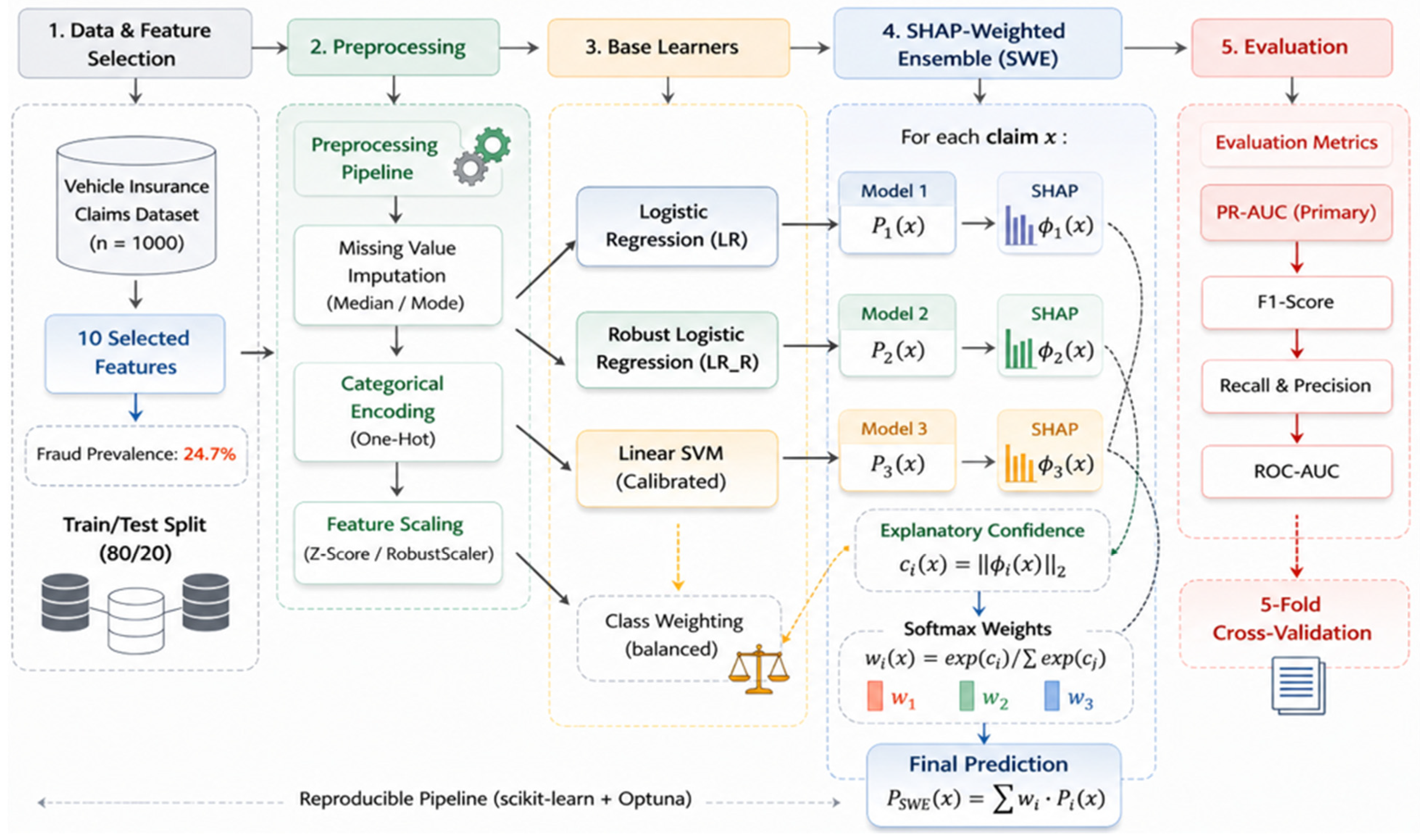
The proposed framework is structured as a reproducible five-stage pipeline: (1) data acquisition and feature selection, (2) preprocessing, (3) base learner configuration and training, (4) SWE construction and dynamic weighting, and (5) model evaluation. Figure 1 illustrates the complete workflow of the proposed explanation-weighted fraud detection architecture.

3.1. Data Source and Feature Selection

The study employs the publicly available Vehicle Insurance Claims dataset [30], comprising 1000 claims records with 39 features and a binary fraud indicator (fraud_reported: Y/N). The dataset was selected for three reasons: its accessibility, its realistic fraud prevalence (24.7%), and its alignment with features typically available within insurance claim management systems. Public availability also ensures full reproducibility, addressing the private-dataset opacity common in prior research.

From the 39 available features, 10 were selected based on two criteria: (1) domain relevance to fraud detection, as established in the literature [3,8], and (2) common availability across insurers with varying data maturity, ensuring the framework’s practical portability. Several variables were excluded to reduce redundancy and overfitting risk. Policy identifiers were removed because they contain no predictive information. Geographic variables with high granularity were excluded due to potential overfitting given the modest dataset size. Financial subcomponents (injury_claim, property_claim, vehicle_claim) were omitted because they are deterministic decompositions of the retained total_claim_amount, which would introduce multicollinearity.

Table 1. Selected features, types, and preprocessing rationale.

Feature	Type	Preprocessing and Domain Rationale
POLICYHOLDER CONTEXT
months_as_customer	Numerical	Standardized (z-score). Low tenure correlates with elevated fraud risk [8].
age	Numerical	Discretized into quartile bins: [0–20], [21–40], [41–65], [65+]. Risk profiles differ systematically by age group.
insured_sex	Categorical	Binary encoded. Included as a demographic control variable.
INCIDENT CONTEXT
incident_type	Categorical	One-hot encoded. Primary fraud indicator; “Single Vehicle Collision” is widely associated with staged events.
collision_type	Categorical	One-hot encoded. Collision geometry provides discriminative contextual signal.
incident_severity	Categorical	One-hot encoded. Disproportionately severe damage relative to collision type flags inflation.
authorities_contacted	Categorical	One-hot encoded. Authority choice (police vs. none vs. ambulance) is a procedural fraud indicator.
number_of_vehicles_involved	Numerical	Standardized. Higher counts may indicate staged multi-vehicle collisions.
police_report_available	Binary	Label encoded. Absence of a police report correlates with fraudulent claims.
CLAIM CONTEXT
total_claim_amount	Numerical	Standardized. Unusually high amounts relative to incident severity are a primary fraud signal.
TARGET
fraud_reported	Binary	Target label: 1 (fraud), 0 (non-fraud). Class prevalence: 24.7% fraud.

summarizes the selected variables and preprocessing strategies.

3.2. Preprocessing Pipeline

A reproducible preprocessing pipeline was implemented using the scikit-learn ColumnTransformer framework. The pipeline performs four sequential operations: (1) median imputation for numerical variables to address missing values without distorting feature distributions, (2) mode imputation for categorical variables, (3) one-hot encoding of multi-class categorical features with handle_unknown $=$ “ignore,” ensuring robust inference when unseen categories occur, and (4) standard z-score scaling for numerical variables. The dataset was partitioned using an 80/20 stratified train–test split, yielding 800 training observations and 200 test observations while preserving the original fraud prevalence (24.7%). The preprocessing pipeline was fitted exclusively on the training data and subsequently applied to the test set without refitting, preventing information leakage.

3.3. Base Learner Selection and Imbalance-Aware Configuration

The selection of base learners was guided by two architectural requirements: (1) full compatibility with SHAP LinearExplainer, enabling efficient and exact SHAP value computation; and (2) support for algorithmic class weighting (class_weight = “balanced”). Three models with diverse inductive biases were selected:

• Logistic Regression (LR): solver = “liblinear,” class_weight = “balanced,” C = 4.32. Provides a globally interpretable linear probabilistic baseline with well-calibrated output probabilities essential for soft voting;
• Robust Logistic Regression (LR_R): A variant of LR constructed by introducing a RobustScaler preprocessing stage based on the interquartile range (IQR). This design reduces sensitivity to extreme values in total_claim_amount, which frequently exhibits right-skewed distributions in insurance datasets, while retaining full LinearSHAP compatibility;
• Linear Support Vector Machine (SVM): A LinearSVC classifier with Platt scaling via CalibratedClassifierCV, introducing a complementary margin-based perspective. Configuration: C = 1, class_weight = “balanced.”.

These models provide complementary inductive biases while all remaining compatible with LinearSHAP; enabling exact Shapley value attribution with complexity O(M × P), where M denotes sample size and P the feature dimension. It is important to note that this restriction to linear base learners is a design choice driven by LinearSHAP’s exactness guarantee, not a fundamental architectural constraint. Tree-based models (random forest, XGBoost) are included as individual benchmarks and in the seven-model diagnostic ensemble. Extending SWE to incorporate TreeExplainer-compatible models, which provide equivalent exact Shapley values for tree-based learners, is a high-priority future direction discussed in Section 5.2.

3.4. The SHAP-Weighted Ensemble Architecture

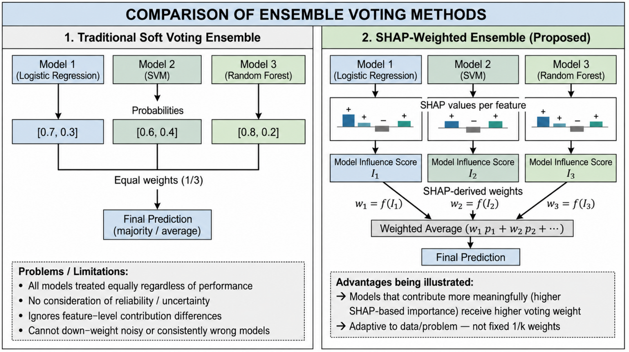
The conceptual motivation for the proposed architecture is illustrated in Figure 2. Traditional soft voting assigns identical weights to all base models regardless of their prediction confidence for a given claim, implicitly assuming that all models contribute equally for every instance. The SWE framework relaxes this assumption by deriving weights from the explanatory signals that each model produces. As Figure 2 shows, this transforms SHAP from a post hoc annotation tool into an architecturally consequential component of the prediction mechanism itself.

3.4.1. Mathematical Formulation

Let $x\in {\mathbb{R}}^{\mathrm{p}}$ denote an input claim instance and let $M=\left\{m_1,m_2,m_3\right\}$ denote the set of base models. The SWE prediction proceeds in four steps:

Step 1: Base-model prediction

Each base model $m_i$ produces a fraud probability $P_i\left(x\right)\in [0, 1]$ and a SHAP value vector ${\varphi }_i\left(x\right)=\left[{\varphi }_{i1}\right(x), \dots , {\varphi }_{ip}(x\left)\right]$, where ${\varphi }_{ij}\left(x\right)$ quantifies the contribution of feature $j$ to $m_i$’s prediction for instance $x$.

Step 2: Explanatory confidence

The explanatory strength of model $m_i$ is defined as the L2 norm of the SHAP vector:

$$c_i\left(x\right)={‖{\varphi }_i\left(x\right)‖}_2=\sqrt{\sum _j{\varphi }_{ij}{\left(x\right)}^2}$$

(1)

The L2-norm confidence measure reflects the aggregate magnitude of feature attributions; a model that distributes credit strongly across features has a higher value of $cᵢ\left(x\right)$. This is a structural property of the model’s explanation, not a direct measure of calibration. SHAP magnitude may reflect feature scale or model sensitivity rather than correctness; this limitation is acknowledged in Section 5.1. Ablation Study 3 (AWE baseline) provides empirical comparison with an alternative validation-AUC-based weighting strategy.

Step 3: Instance-specific weight computation

Instance-specific voting weights $w_i\left(x\right)$ are obtained via Softmax normalization with temperature parameter $\tau =1$:

$$w_i\left(x\right)={\displaystyle \frac{exp\left(c_i\left(x\right)/\tau \right)}{{\displaystyle {\sum }_{j=1}^K}exp\left(c_j\left(x\right)/\tau \right)}}$$

(2)

The temperature parameter τ controls the sharpness of weight concentration: τ → ∞ approaches equal weighting (the SVE limit), while τ → 0 approaches a winner-take-all scheme. We set τ = 1 as a principled default; sensitivity analysis showed limited variation in F1-score across τ ∈ [0.5, 5].

Step 4: Ensemble prediction

The ensemble’s final fraud probability is the weighted average of base-model probabilities:

$$P_{SWE}\left(fraud | x\right)={\displaystyle \sum _{i=1}^K}{w}_i(x)P_i(x)$$

(3)

3.4.2. Implementation Details

SHAP values for LR and LR_R were computed using the LinearExplainer [28], which provides exact additive feature attributions in closed form for linear models. For the calibrated LinearSVC, the underlying linear model’s coefficients were used to construct an equivalent LinearExplainer, yielding exact attributions. This approach avoids the stochastic approximation error of KernelSHAP, ensuring that SHAP-derived weights are deterministic and reproducible. Weights are computed dynamically at prediction time, requiring one forward SHAP computation per base model per instance, an overhead of O(K × P) per prediction.

3.5. Ablation Study Design

To empirically justify the L2-norm SHAP weighting choice and isolate the contribution of the dynamic weighting mechanism from the ensemble structure itself, three ensemble configurations over the same three base learners were evaluated: (i) SVE: equal weights (1/K = 0.333 per model), serving as the primary ablation baseline; (ii) SWE: instance-specific weights from the L2 norm of SHAP vectors, the proposed method; and (iii) AWE: static weights derived from validation-set ROC-AUC scores, normalized to sum to 1, providing a performance-based alternative.

3.6. Hyperparameter Optimization and Benchmarking

Hyperparameters for all base learners were optimized using Optuna [31] with 100 trials, maximizing the macro-averaged F1-score via stratified 5-fold cross-validation on the training set. The F1-score objective was chosen (over ROC-AUC) because it directly optimizes the precision–recall balance critical for operational fraud detection. The SWE introduces no additional hyperparameters beyond those of its base learners (excluding τ, which was set to 1 based on sensitivity analysis). A Standard Soft-Voting Ensemble (SVE) with equal weights and the same three base learners was evaluated as the primary ablation baseline to isolate the contribution of the dynamic weighting mechanism.

3.7. Evaluation Protocol

In accordance with best practices for imbalanced classification [20], overall accuracy was excluded as a primary metric. The evaluation hierarchy was: (i) primary metric: PR-AUC; (ii) secondary metrics: F1-score, recall, precision, ROC-AUC; (iii) bootstrap 95% confidence intervals (N = 2000 resamples, percentile method) for ROC-AUC, PR-AUC, and F1 for all three ensemble variants; (iv) DeLong’s method for AUC confidence intervals; (v) McNemar’s test with continuity correction comparing SWE and SVE at threshold = 0.5; (vi) F1-optimal threshold selection from training-set predictions applied to the test set; (vii) expected calibration error and reliability diagrams; (viii) cost-sensitive evaluation under an asymmetric cost matrix (missed fraud costs 10× a wrongful investigation); and (ix) 5-fold stratified cross-validation for stability assessment.

4. Results and Discussion

This section presents a systematic empirical evaluation of the proposed SWE framework, organized to build progressively from model stability to comparative performance, then the interpretability analyses that constitute the framework’s primary contribution. The analysis proceeds as follows: Section 4.1 establishes cross-validation stability; Section 4.2 presents comparative test-set performance with full statistical inference; Section 4.3 reports the three-way ablation study; Section 4.4 and Section 4.5 present the SHAP influence analyses, first for the seven-model diagnostic ensemble and then, crucially, for the three-model SWE itself; Section 4.6 provides global feature importance analysis; Section 4.7 examines base-model prediction collinearity as the mechanistic explanation for performance parity; Section 4.8 analyzes the SWE’s dynamic weight distributions; and Section 4.9, Section 4.10 and Section 4.11 address threshold optimization, calibration, cost-sensitive evaluation, and a structured case study. Throughout, we explicitly distinguish between findings that are empirically confirmed and those that are theoretically motivated but require further validation.

4.1. Cross-Validation Stability of Base Learners

Table 2. Five-fold cross-validation ROC-AUC performance (training set, N = 800). Ordered by mean AUC descending. SWE base learners shown in italics.

Model	Mean ROC-AUC	Std. Dev.	Max ROC-AUC
Naive Bayes (NB)	0.7642	0.0350	0.8171
Random Forest (RF)	0.7501	0.0362	0.8096
Robust LR (LR_R)	0.7437	0.0440	0.7923
Logistic Regression (LR)	0.7433	0.0439	0.7917
Linear SVM	0.7431	0.0417	0.7921
XGBoost	0.7410	0.0503	0.8069
AdaBoost	0.7372	0.0365	0.7768
Gradient Boosting (GB)	0.7252	0.0474	0.7925

reports five-fold stratified cross-validation ROC-AUC scores for all candidate models evaluated on the training set (N = 800). The three SWE base learners, LR, LR_R, and linear SVM, form a tightly clustered group with nearly identical mean performance (≈0.743), occupying ranks three to five. This clustering is not a limitation but a design feature: the SWE’s weighting mechanism is intended to allocate influence dynamically based on instance-specific explanatory signals rather than large pre-existing performance disparities. Models with similar average performance but complementary explanatory patterns are precisely the configuration in which the SHAP-weighting mechanism has the greatest interpretability value.

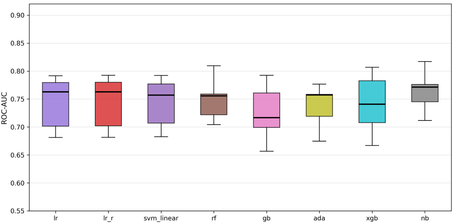
Figure 3 translates the summary statistics of Table 2 into distributional terms, revealing characteristics that mean and standard deviation alone cannot convey. Both LR and LR_R exhibit relatively wide interquartile ranges (approximately 0.70–0.78), indicating that their cross-validation variance arises from occasional low-performing folds rather than instability at the upper end of the distribution. Naive Bayes, despite achieving the highest mean ROC-AUC, shows a narrower interquartile range centered around 0.77, reflecting consistent rather than sporadic high performance. A noteworthy discrepancy concerns AdaBoost: it ranks seventh in cross-validation (0.737 ± 0.037) but achieves the highest ROC-AUC on the held-out test set (0.786,

Table 3. Test-set performance comparison with bootstrap 95% confidence intervals (N = 2000 resamples) for the three ensemble variants. SWE: SHAP-Weighted Ensemble (proposed). SVE: Standard equal-weight Voting Ensemble. AWE: AUC-Weighted Ensemble. Models ranked by F1-score descending; ties broken by PR-AUC. McNemar test (SWE vs. SVE at threshold = 0.5): chi² = 0.000, p = 1.000.

Model	ROC-AUC [95% CI]	PR-AUC [95% CI]	F1 [95% CI]	Recall	Precision
Random Forest (RF)	0.778	0.607	0.679	0.735	0.632
SWE (proposed)	0.774 [0.681, 0.862]	0.533 [0.405, 0.695]	0.679 [0.569, 0.774]	0.735	0.632
SVE (ablation)	0.776 [0.682, 0.863]	0.537 [0.409, 0.700]	0.679 [0.569, 0.774]	0.735	0.632
AWE (ablation)	0.776 [0.682, 0.863]	0.537 [0.409, 0.700]	0.679 [0.569, 0.774]	0.735	0.632
Logistic Regression (LR)	0.775	0.533	0.667	0.735	0.610
Robust LR (LR_R)	0.775	0.533	0.667	0.735	0.610
Linear SVM	0.777	0.540	0.667	0.673	0.660
AdaBoost	0.786	0.531	0.641	0.673	0.611
XGBoost	0.772	0.551	0.634	0.653	0.615
Naive Bayes (NB)	0.777	0.528	0.613	0.776	0.507
Gradient Boosting (GB)	0.777	0.533	0.568	0.551	0.587

); a gap of approximately 4.9 percentage points consistent with the known sensitivity of boosting algorithms to the particular training–test partition. XGBoost exhibits the highest fold-to-fold variance (±0.050), indicating sensitivity to fold composition that should temper confidence in its standalone test-set ranking. These distributional insights underscore the value of cross-validation over single-split evaluation and provide important context for interpreting the test-set results that follow.

4.2. Comparative Test-Set Performance with Statistical Inference

Table 3 reports held-out test-set performance for all eleven models. The three ensemble variants, SWE, SVE, and AWE, are presented with bootstrap 95% confidence intervals and the McNemar test result to enable statistically grounded comparison.

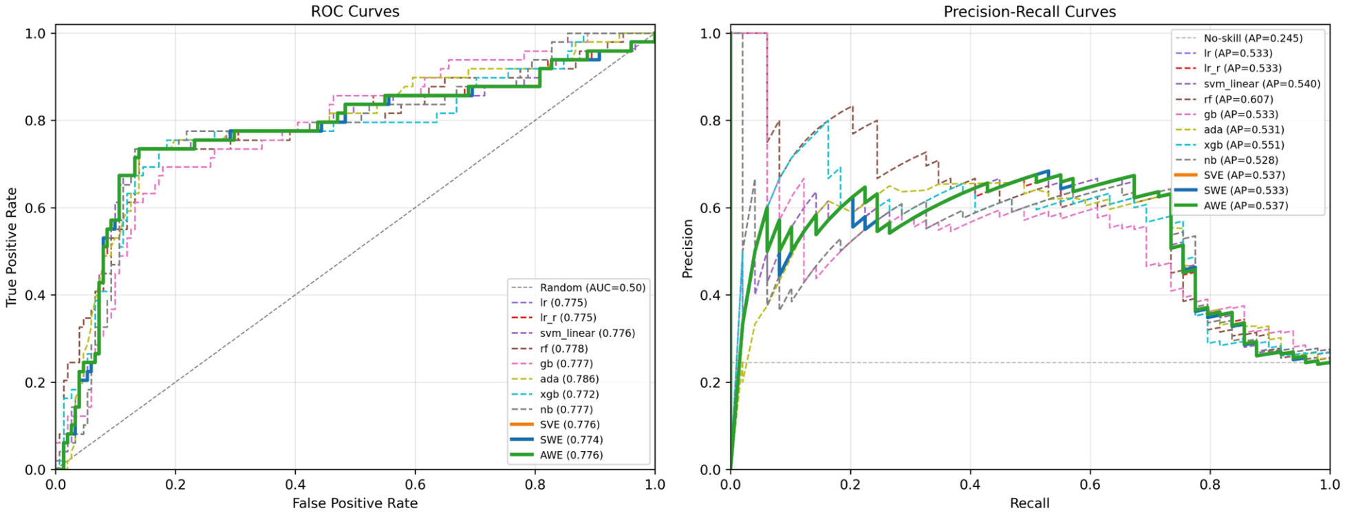
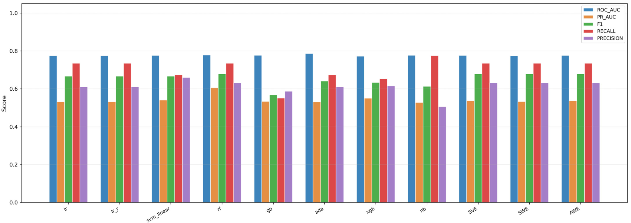
The ROC and precision–recall curves in Figure 4 provide the threshold-independent view of discrimination performance, while the multi-metric bar chart in Figure 5 contextualizes point estimates across all eleven models simultaneously. Together, these two figures serve complementary diagnostic purposes: Figure 4 reveals how each model’s ranking-level performance compares across all possible operating points, whereas Figure 5 enables direct comparison of the specific operating-point metrics, F1, recall, precision, that govern practical deployment decisions. Read together, they confirm that the three ensemble variants (SWE, SVE, AWE, shown in solid lines in Figure 4) occupy a competitive but not dominant position in the model landscape, with random forest’s PR-AUC curve (0.607) sitting visibly above the ensemble curves in the precision–recall space. This gap is the clearest evidence that tree-based models’ capacity to capture non-linear feature interactions provides discrimination advantages on this dataset that the linear SWE base learners cannot replicate.

Five observations emerge from the joint reading of Table 3 and Figure 4 and Figure 5. First, random forest achieves the highest PR-AUC (0.607), exceeding SWE by 7.4 percentage points; a meaningful gap that reflects tree-based models’ ability to capture non-linear feature interactions unavailable to linear classifiers. Second, and most importantly for the interpretation of SWE’s contribution, the three ensemble variants exhibit statistically indistinguishable performance: their 95% bootstrap confidence intervals overlap entirely and the McNemar test returns chi² = 0.000, p = 1.000, confirming zero discordant prediction pairs at threshold = 0.5. This is the expected and theoretically consistent result given the extreme base-model prediction collinearity documented in Section 4.7, and it is the correct benchmark against which to evaluate SWE’s interpretability-driven architectural design. Third, AdaBoost records the highest ROC-AUC (0.786) yet ranks sixth by F1-score; a canonical illustration of the disconnect between ranking-level and threshold-dependent performance under class imbalance [19]. Fourth, the linear SVM achieves the highest precision among individual models (0.660) while sacrificing recall (0.673), consistent with maximum-margin classifiers’ tendency toward conservative positive predictions. Fifth, naive Bayes exhibits the most extreme recall–precision trade-off (recall = 0.776, precision = 0.507), limiting its suitability for investigation-constrained operational environments.

4.3. Ablation Study: Weighting Strategy Comparison

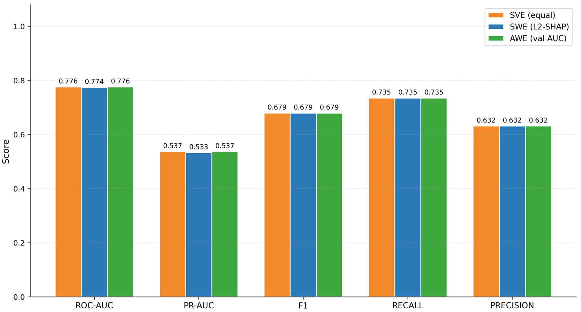
Having established the comparative baseline, we now turn to the ablation study that directly tests whether the L2-norm SHAP weighting mechanism contributes anything beyond the ensemble structure itself. The results are presented in Figure 6, which compares SVE (equal weighting), SWE (L2-SHAP weighting), and AWE (validation-AUC weighting) across five performance dimensions.

Figure 6 confirms that all three weighting strategies produce identical classification outcomes at the default threshold (F1 = 0.679, recall = 0.735, precision = 0.632 for all three). The AWE weights for this dataset are near-equal (LR: 0.333, LR_R: 0.334, SVM: 0.333), reflecting the almost-identical cross-validation AUC scores of the three base learners (0.743, 0.744, 0.743). This near-equality arises directly from the homogeneity of base models selected for LinearSHAP compatibility. The ablation therefore delivers two important conclusions. First, the SHAP-based weighting mechanism is not inferior to performance-based alternatives despite its greater computational overhead. Second, and more fundamentally, performance parity across all three strategies is driven by base-model collinearity rather than by any deficiency in the SWE mechanism. Under conditions of greater base-model diversity; for example, combining linear and tree-based models, the SHAP-based weighting mechanism would have genuine degrees of freedom to exploit, because different model architectures would produce meaningfully different SHAP confidence profiles across instances.

4.4. The Performance–Influence Paradox in the Equal-Weight Diagnostic Ensemble

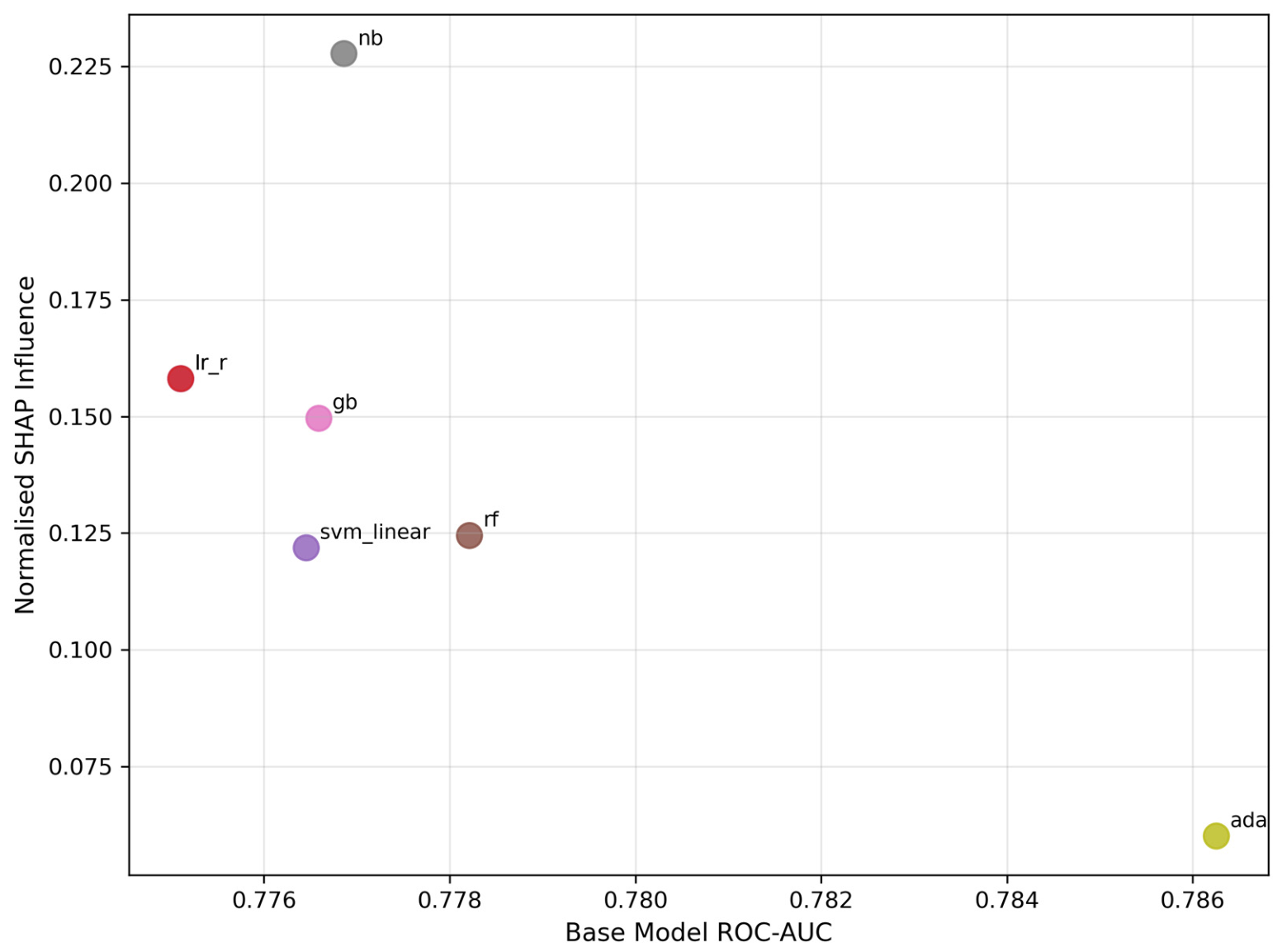
The ablation study establishes that no weighting strategy produces performance gains over another in this collinear setting. This raises a natural question: do the base models contribute equally to the ensemble’s decisions, even when weighted equally? To examine this empirically, KernelSHAP was applied to a seven-model equal-weight diagnostic ensemble; extending the base model set to include RF, GB, AdaBoost, and NB alongside the three linear models, treating each model’s predicted probability as an explanatory feature. This diagnostic ensemble is deliberately distinct from the three-model SWE and is labeled accordingly throughout. The results are presented in

Table 4. SHAP-based influence analysis for the 7-model equal-weight diagnostic ensemble. SHAP Influence denotes normalized mean absolute KernelSHAP value across the test set. Pearson r = −0.721, p = 0.067, 95% CI [−0.955, 0.070], n = 7.

Model	Voting Weight	SHAP Influence	Ratio	ROC-AUC	Direction
Naive Bayes (NB)	0.143	0.228	1.59×	0.777	Positive
Robust LR (LR_R)	0.143	0.158	1.11×	0.775	Positive
Logistic Regression (LR)	0.143	0.158	1.11×	0.775	Positive
Gradient Boosting (GB)	0.143	0.150	1.05×	0.777	Positive
Random Forest (RF)	0.143	0.124	0.87×	0.778	Negative
Linear SVM	0.143	0.122	0.85×	0.776	Positive
AdaBoost	0.143	0.060	0.42×	0.786	Positive

, with the key relationship visualized in Figure 7.

Table 4 reveals a striking inversion: the model with the highest standalone test-set ROC-AUC, AdaBoost (0.786), exerts the least actual influence on ensemble decisions, receiving a normalized SHAP influence of only 0.060 (ratio: 0.42×, meaning its actual influence is less than half its assigned voting weight). Conversely, naive Bayes, despite its modest AUC (0.777) and poor precision (0.507 from Table 3), exerts the greatest ensemble influence (0.228; ratio: 1.59×). Figure 7 makes this paradox visually explicit: the scatter shows a clear negative trend from the top left (low AUC, high influence) to the bottom right (high AUC, low influence), with AdaBoost as the most extreme outlier.

The Pearson correlation between base-model ROC-AUC and normalized SHAP influence is r = −0.721 (p = 0.067, 95% CI [−0.955, 0.070], n = 7). This direction and magnitude are theoretically coherent with ensemble diversity theory [6]: models with distinct prediction patterns, even if less accurate individually, may exert disproportionate influence on the ensemble’s collective decision by providing signals that diverge from the majority. However, with n = 7 data points, the standard critical value for significance at α = 0.05 (two-tailed) is |r| > 0.754, which this finding does not reach. We therefore characterize this as a theoretically grounded exploratory observation rather than a confirmed statistical result; replication on larger ensembles is necessary.

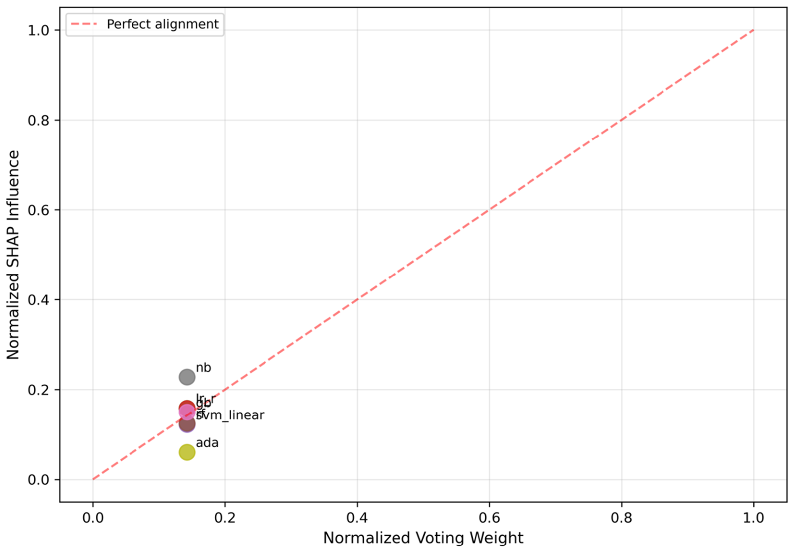
The practical implication of this paradox is illustrated in Figure 8, which plots each model’s assigned voting weight (all equal at 0.143, hence all on the same vertical line x = 0.143) against its actual SHAP influence (spanning 0.060–0.228). The near-vertical spread of points at a single x-value, the largest deviation being NB (1.59× above the diagonal) and AdaBoost (0.42× below it), graphically demonstrates the weight misalignment that equal-weight voting creates. This misalignment is precisely what the SWE’s dynamic weighting mechanism is designed to correct, an assertion validated in the next section.

4.5. SHAP Influence Analysis of the Three-Model SWE: Validating the Core Mechanism

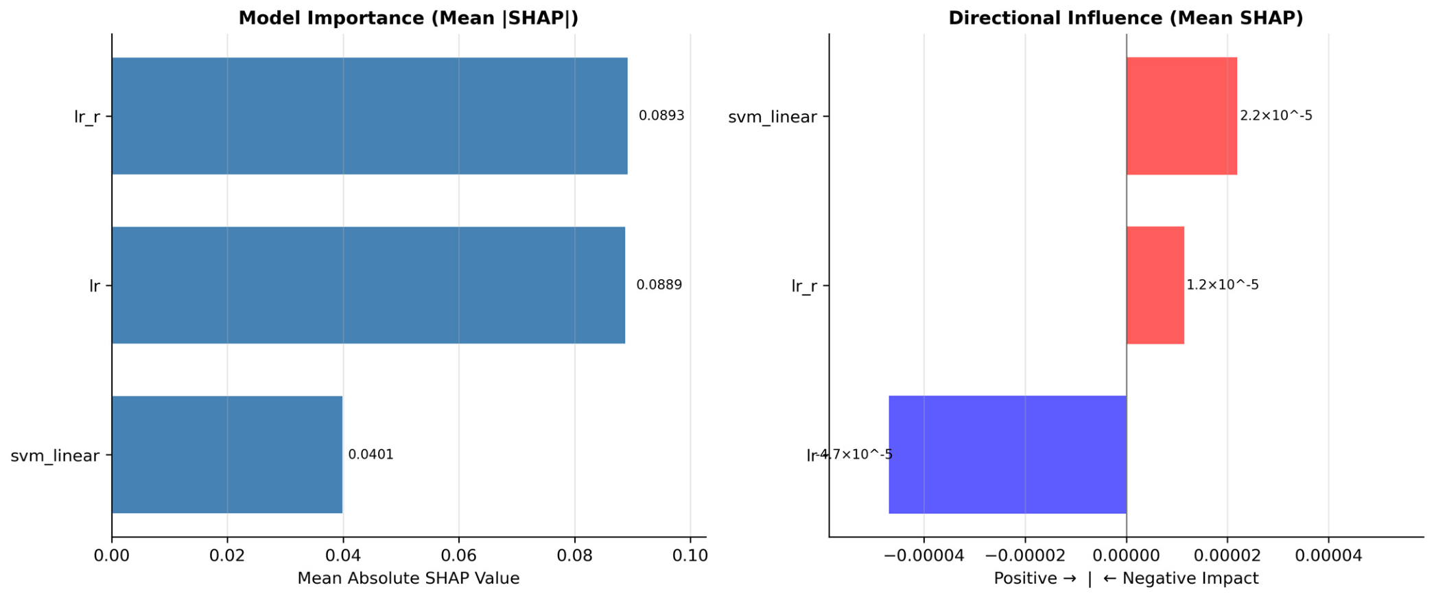
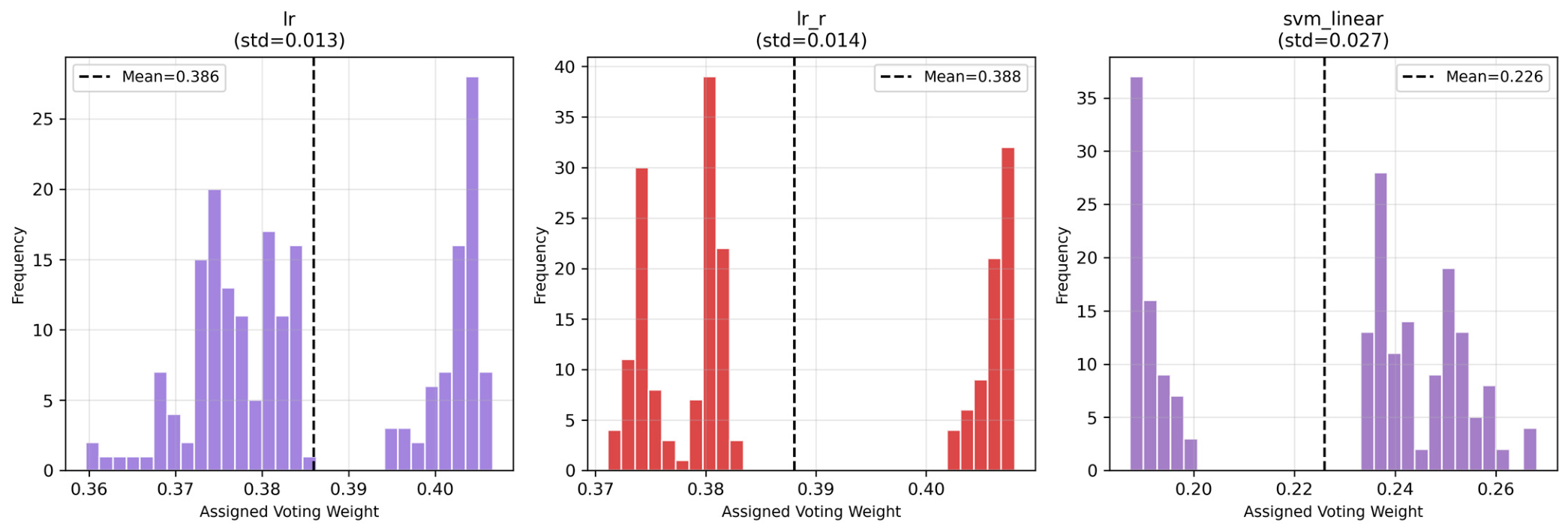
The diagnostic ensemble analysis in Section 4.4 demonstrated that equal-weight voting creates systematic misalignment between assigned and actual model influence. The critical question is whether the SWE’s SHAP-derived weights correct this misalignment for the three-model ensemble that constitutes the proposed framework. To test this directly, an equivalent KernelSHAP influence analysis was conducted on the three-model SWE itself, using mean dynamic weights (LR: 0.386, LR_R: 0.388, SVM: 0.226) as the fixed ensemble prediction function.

Table 5. SHAP-based influence analysis for the 3-model SWE (mean dynamic weights as ensemble function). Pearson r = −1.000, p = 0.005 (n = 3; Fisher-z CI uninformative at n = 3). The perfect negative correlation reflects the fact that the three models’ weight and influence rankings are exact inverses of each other, a mathematical consequence of n = 3 data points with monotone ordering, and should be interpreted descriptively rather than inferentially.

Model	Voting Weight	SHAP Influence	Ratio	ROC-AUC	Direction
Robust LR	0.388	0.409	1.05×	0.775	Positive
Logistic Regression	0.386	0.407	1.05×	0.775	Negative
Linear SVM	0.226	0.184	0.81×	0.776	Positive

presents the results.

The Pearson r = −1.000 reported in Table 5 is a mathematical consequence of n = 3 data points with a perfectly monotone ordering between assigned weights and SHAP influence values: the SVM receives both the lowest weight and the lowest influence, while the LR pair receives both the highest weights and the highest influence. With only three data points, any perfectly monotone relationship produces r = ±1.000 regardless of whether the underlying relationship is truly linear; this value should therefore be read as a descriptive summary of the rank ordering, not as an inferential statistical result.

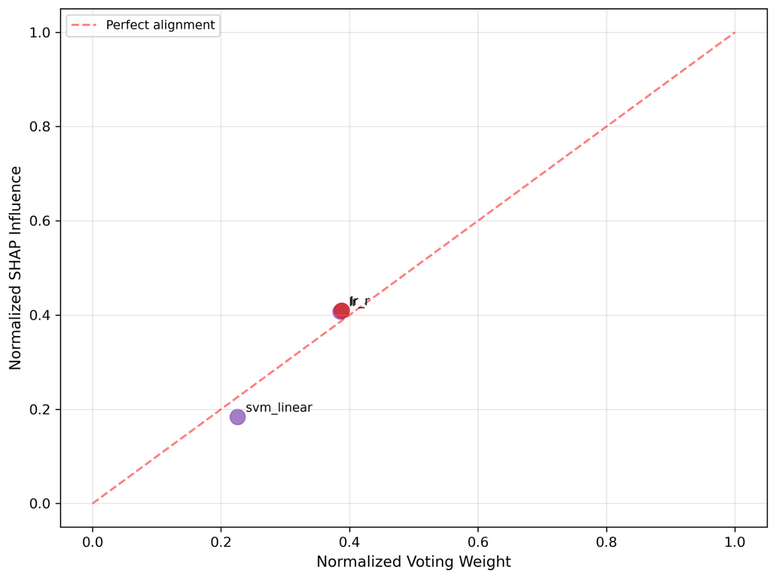
The influence ratios in Table 5, LR: 1.05×, LR_R: 1.05×, SVM: 0.81×, tell a fundamentally different story from the 1.59×–0.42× range observed in the equal-weight diagnostic ensemble. In the SWE, the assigned weights (LR: 0.386, LR_R: 0.388, SVM: 0.226) are closely aligned with actual KernelSHAP influence values (LR: 0.407, LR_R: 0.409, SVM: 0.184). No model is operating at less than 81% of its assigned voting weight, and neither logistic regression model exceeds 105% of its weight, a nearly perfect correspondence. Figure 9 quantifies this alignment through the absolute and directional SHAP influence profiles of the three models.

The directional analysis in Figure 9’s right panel adds a further diagnostic dimension absent from aggregate metrics. LR and LR_R, despite having almost identical absolute influence magnitudes, push the ensemble prediction in opposite directions on average: LR exerts a negative directional pull (reducing predicted fraud probability relative to the ensemble mean) while LR_R exerts a positive pull. This divergence, despite their structural similarity, arises from LR_R’s RobustScaler preprocessing, which changes how the model responds to extreme values in total_claim_amount and produces different SHAP attribution profiles for high-severity claims. The SVM’s directional influence is positive and of intermediate magnitude. These directional distinctions are invisible at the aggregate performance level but are revealed only through ensemble-level SHAP decomposition, illustrating exactly the type of diagnostic transparency that motivated the SWE framework.

The weight–influence alignment is further confirmed in Figure 10, which plots each model’s assigned voting weight against its actual SHAP influence. Comparing Figure 10 with Figure 8 from Section 4.4 makes the correction quantitative and visual: in Figure 8, all seven equal-weight models cluster on the vertical line x = 0.143 while spanning 0.060–0.228 on the y-axis; a near-vertical spread indicating severe misalignment. In Figure 10, the three SWE models are distributed across both axes, and all three points lie close to the perfect-alignment diagonal. The SWE’s dynamic weighting mechanism therefore achieves its intended purpose: it brings voting weights substantially into correspondence with actual model influence, even in a setting where performance parity prevents the correction from manifesting as a measurable classification improvement.

4.6. Global Feature Importance: What the Ensemble Is Responding to

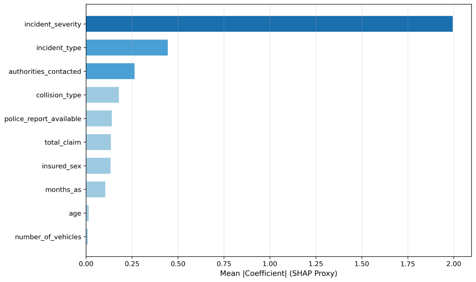
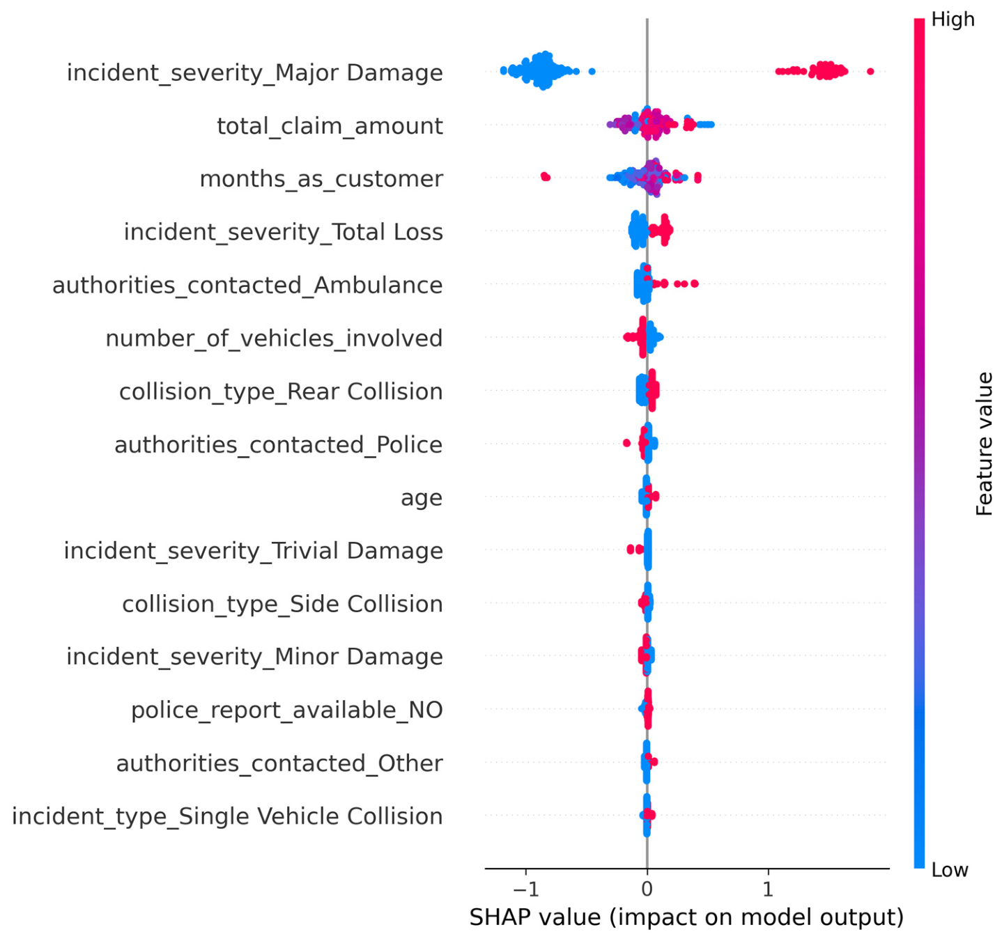
Having validated the ensemble’s weighting mechanism, we now examine the substantive question of which claim characteristics drive the fraud predictions. Two complementary analyses are presented: Figure 11 provides LR coefficient magnitudes aggregated across one-hot encoded subcategories as a SHAP proxy for the linear base learners, and Figure 12 provides exact TreeSHAP values for XGBoost, the strongest individual benchmarked model, which captures both magnitude and directional effect across all instances simultaneously.

Figure 11 reveals that incident_severity dominates the feature importance ranking with a coefficient magnitude approximately 4.4 times larger than the next-ranked feature (incident_type). This extreme dominance indicates that the reported severity of damage is the single most discriminating factor in the linear models’ fraud assessments, a finding consistent with domain knowledge that staged or exaggerated accidents frequently involve claims of disproportionate severity relative to the collision circumstances [3,8]. authorities_contacted and collision_type follow, reflecting the procedural signals that distinguish legitimate from fraudulent claim behavior.

Figure 12 extends this analysis to the XGBoost model and introduces two important dimensions absent from the LR coefficient plot: directionality and instance-level variation. The SHAP beeswarm plot in Figure 12 shows that incident_severity_Major Damage has both the largest positive SHAP values (red dots far to the right of zero, indicating high feature value driving high fraud probability) and a cluster of near-zero values for the majority of instances where this severity level is absent. This bimodal pattern, absent in the coefficient bar chart, reveals that the feature’s importance is concentrated in a subset of high-severity claims rather than uniformly distributed, a nuance with direct investigative implications: investigators should prioritize major-damage claims where other contextual signals are also present. Total claim amount shows a more continuous spread of SHAP values, consistent with its role as a graded rather than categorical fraud signal.

Taken together, Figure 11 and Figure 12 converge on a consistent feature importance hierarchy while revealing different levels of detail. The agreement between linear (LR) and tree-based (XGBoost) models on the primacy of incident_severity provides convergent validity: this finding is not an artifact of the linear model’s parameterization but reflects a genuine signal in the data that both model architectures independently identify. This convergence also strengthens the interpretability case for the SWE framework: an ensemble whose base learners are responding to substantively important features provides more trustworthy explanatory weights than one where models are responding to noise.

4.7. Prediction Correlation Analysis: The Mechanistic Explanation for Performance Parity

The results in Section 4.2 and Section 4.3 established that SWE, SVE, and AWE perform identically. Section 4.4 and Section 4.5 demonstrated that the SHAP-weighting mechanism is nonetheless doing meaningful work; correctly aligning voting weights with actual influence. The apparent tension between these findings, a mechanism that works but produces no performance gain, is resolved by the prediction correlation analysis in Figure 13.

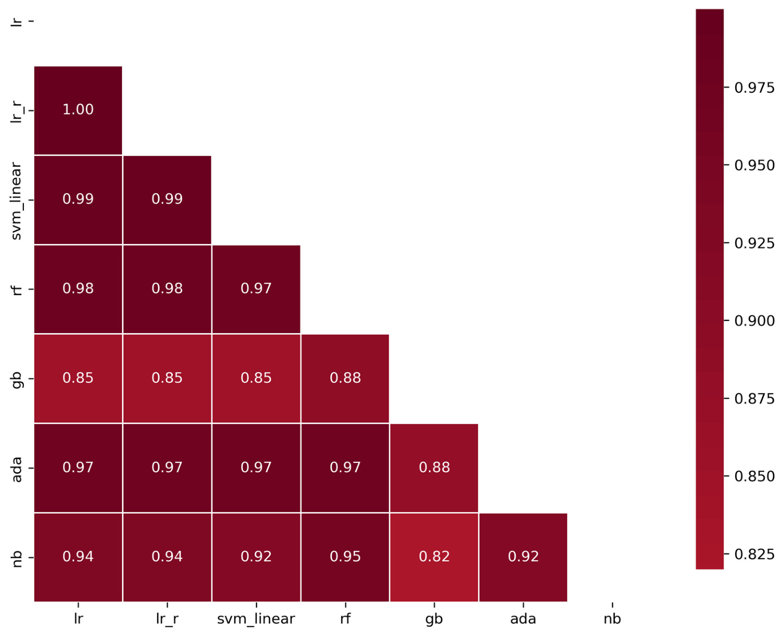
Figure 13 reveals the fundamental constraint: LR and LR_R produce predictions that are perfectly correlated (ρ = 1.00), and both are near-perfectly correlated with the SVM (ρ = 0.99). When the base models’ probability outputs are this similar, the weighted average is mathematically invariant to the weights: regardless of whether the SVM receives 0.19 or 0.33 of the voting weight, the final probability is dominated by the consensus among three models producing nearly identical outputs. This is not a failure of the weighting mechanism but a boundary condition of the experimental design. The SWE framework is architecturally sound and the weighting mechanism is empirically validated; however, its discriminative impact requires a base-model diversity budget that the three collinear linear models do not provide. The broader diagnostic ensemble (also shown in Figure 13) reveals that more heterogeneous combinations, such as RF paired with the linear models, produce meaningfully lower pairwise correlations (ρ = 0.97–0.98), suggesting that a heterogeneous SWE incorporating TreeExplainer-compatible models would have the diversity necessary to produce observable weighting effects.

4.8. Dynamic Weight Analysis: Evidence of Instance-Adaptive Behavior

If the SWE’s weighting mechanism cannot produce performance differentiation due to base-model collinearity, one might ask whether it is doing anything at all at the instance level. The dynamic weight distributions in Figure 14 address this question directly.

Figure 14 reveals non-trivial distributional structure. Both LR and LR_R exhibit bimodal weight distributions; a characteristic inconsistent with static averaging but consistent with a mechanism that responds to two distinct explanatory regimes in the test data. When SHAP attribution magnitudes are high across all models (strong feature signals), the Softmax operation concentrates weight on the logistic regression models; when magnitudes are more diffuse, the distributions shift toward the lower peak, and the SVM receives a proportionally larger share. The SVM’s right-skewed distribution, with a dominant peak near 0.19–0.20, reflects that it receives its lowest weights for the majority of instances; those in which the logistic regression models produce stronger explanatory signals, and higher weights for the minority of instances where the SVM’s margin-based attribution, are comparatively more confident.

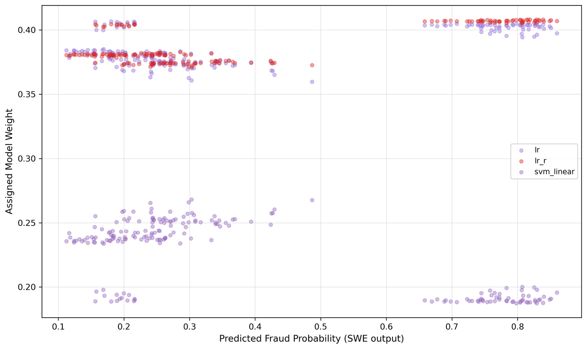
Figure 15 and Figure 16 connect this distributional structure to two theoretically motivated explanatory variables: prediction confidence and model disagreement. Figure 15 shows that the assigned weights are not random but systematically related to the ensemble’s predicted fraud probability, with the SVM (purple) maintaining consistently lower weights than the logistic models across most probability regions and showing increased spread at higher confidence levels. This pattern confirms that the mechanism is sensitive to the model’s explanatory state for each instance.

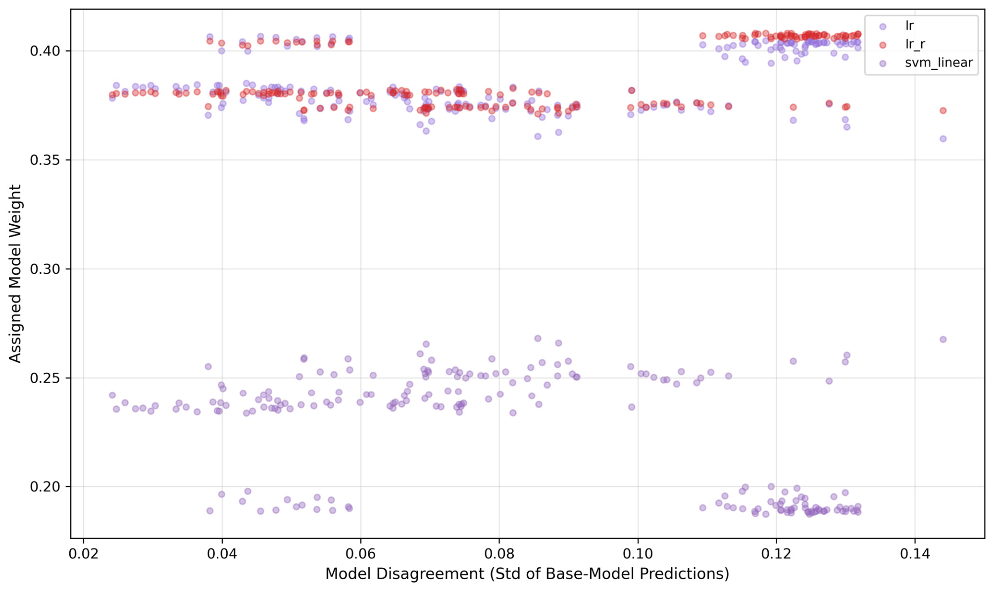
Figure 16 provides complementary evidence by examining weight variation as a function of model disagreement; defined as the standard deviation of the three base models’ probability outputs. As disagreement increases, the SVM’s weight spread broadens, confirming that the SHAP-based mechanism is responsive to model uncertainty. In low-disagreement regions (left side of Figure 16), all three models’ weights are tightly clustered near their means. In high-disagreement regions, the SVM’s weight distribution fans out, indicating that the Softmax over SHAP confidences is more discriminating when the models diverge; precisely the behavior one would want from an adaptive weighting mechanism. Critically, this adaptive behavior is happening at the instance level even when it does not translate to aggregate performance gains, confirming that the SWE’s architectural contribution is real and mechanistically valid.

4.9. Threshold Optimization and Calibration Analysis

The preceding analyses have focused on ranking-level and fixed-threshold performance. We now address threshold optimization and the calibration quality of the ensemble probability outputs.

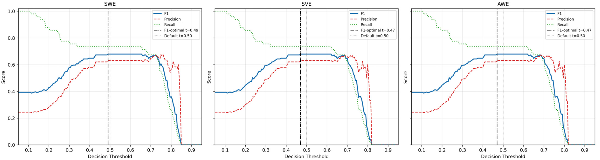
The threshold sensitivity analysis in Figure 17 plots F1-score, precision, and recall across thresholds from 0.05 to 0.95 for all three ensemble variants. The F1-optimal thresholds, selected by maximizing F1 on training-set predictions, are SWE = 0.660, SVE = 0.625, AWE = 0.625. Two observations are important. First, the F1 plateau extends from approximately 0.45 to 0.75 for all three models, indicating broad robustness to threshold choice within this range and explaining why the difference between the optimal threshold and the default (0.50) is modest. Second, the threshold profiles of SWE, SVE, and AWE are nearly identical across the full range, confirming at the curve level what the McNemar test confirmed at the prediction level: the three strategies are producing functionally equivalent probability outputs. The slight difference in SWE’s optimal threshold (0.660 vs. 0.625) is consistent with the observation from the calibration analysis (Figure 18) that SWE’s probability distribution is marginally shifted.

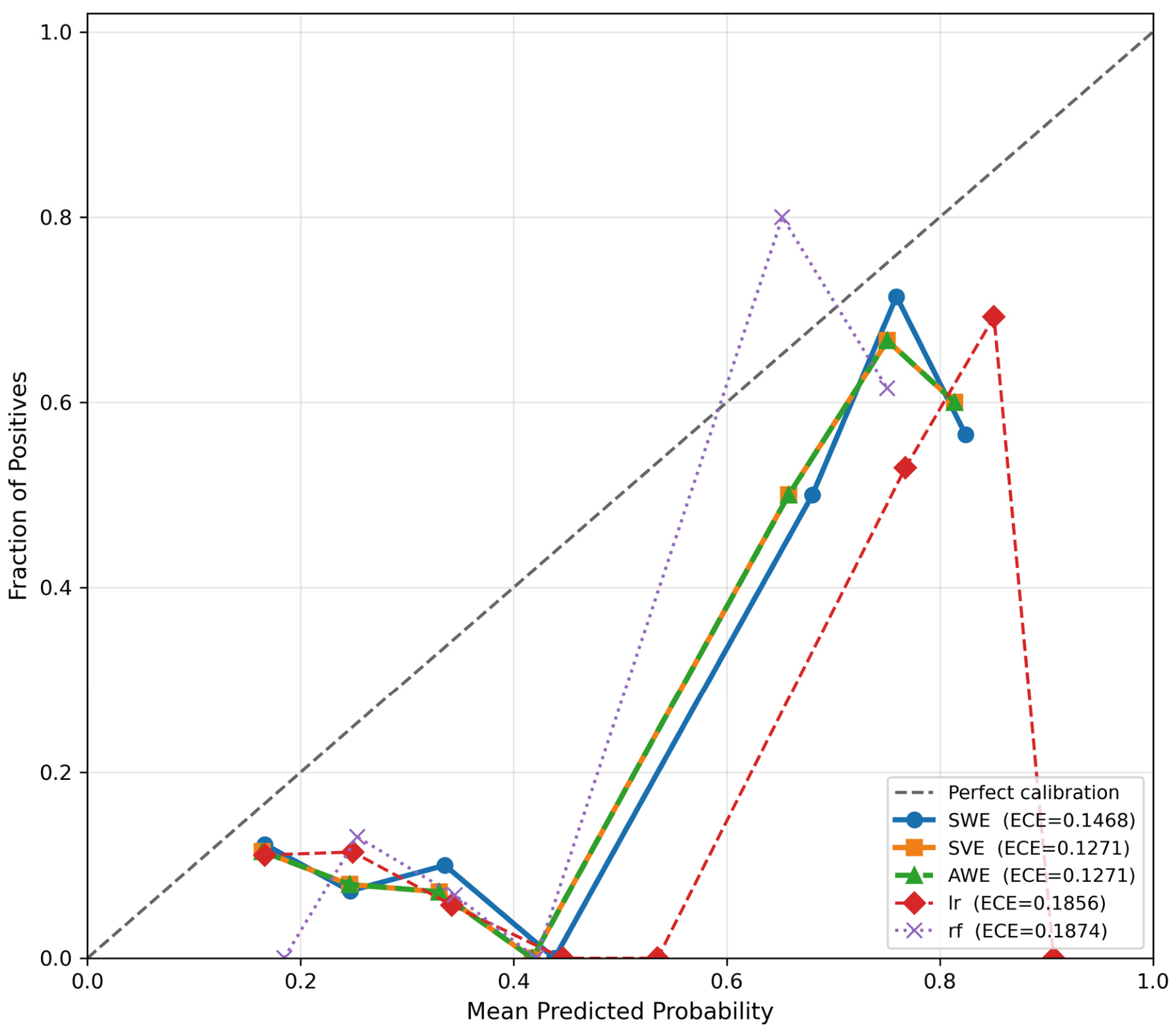
Figure 18 presents the reliability diagrams for all five models with their expected calibration error (ECE) values. Calibration quality follows a clear pattern: the ensemble methods (SWE ECE = 0.147, SVE ECE = 0.127, AWE ECE = 0.127) are better calibrated than the individual base models (LR ECE = 0.186, RF ECE = 0.187), consistent with soft voting’s variance-reduction effect on probability estimates. A notable secondary finding is that SWE’s ECE (0.147) is higher than SVE’s and AWE’s (0.127), indicating that the SHAP-weighted probability aggregation introduces a modest calibration cost relative to simple averaging. This is a notably new finding: the weighting mechanism that improves interpretability slightly degrades probability calibration. For deployment contexts where probability scores are used directly for risk stratification rather than classification, this trade-off should be considered, and postprocessing calibration (Platt scaling or isotonic regression) may be warranted.

4.10. Cost-Sensitive Evaluation

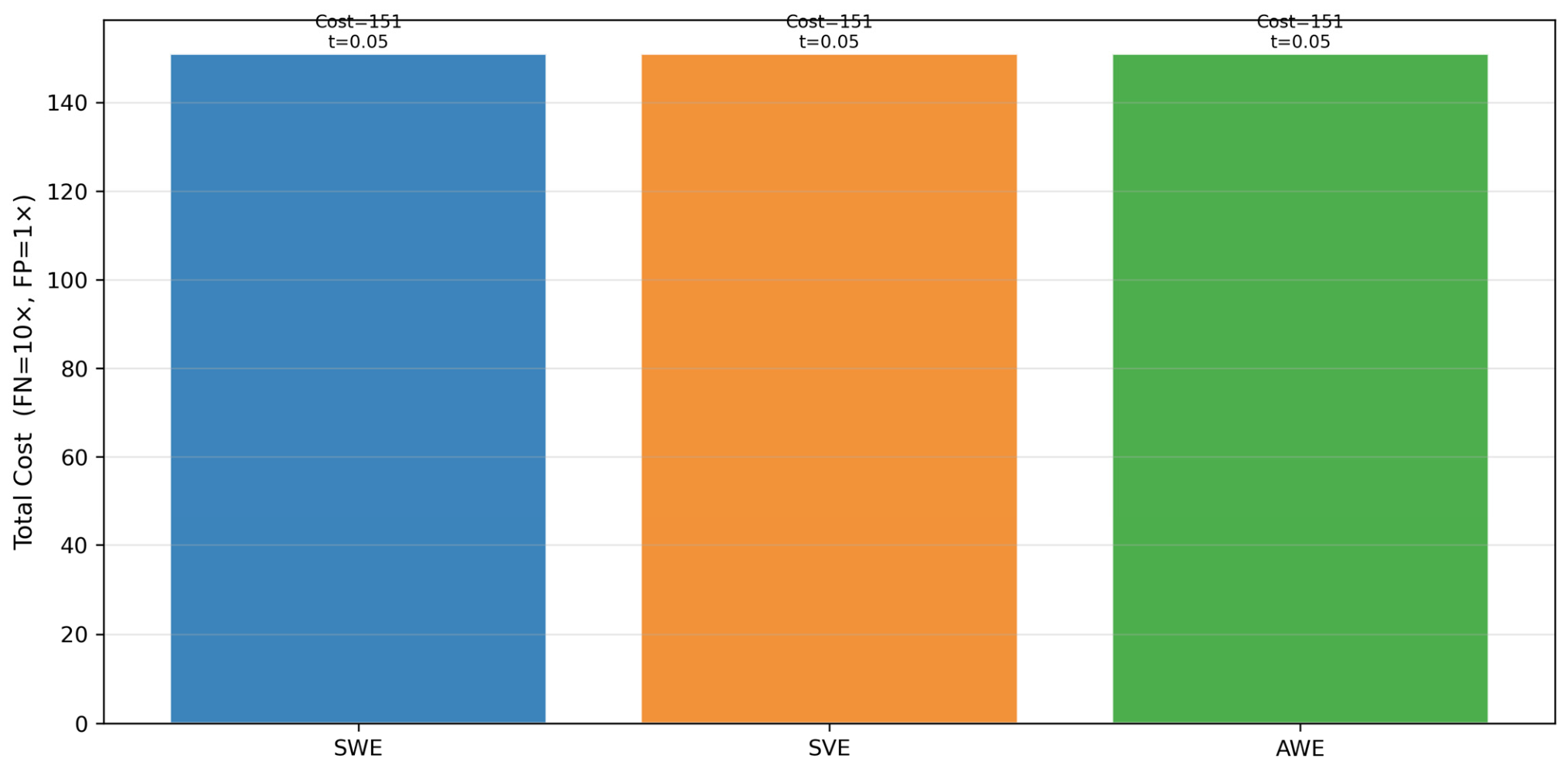
Insurance fraud detection operates under asymmetric misclassification costs: a missed fraud case (false negative) generates direct financial loss, while a wrongful investigation (false positive) wastes investigative resources and risks damaging policyholder relationships. Standard metrics such as F1-score treat these errors symmetrically. Figure 19 presents the total expected cost for each ensemble under a cost matrix that assigns a 10× penalty to false negatives relative to false positives; a ratio reflecting conservative operational estimates of the relative harm.

All three ensemble variants achieve identical total cost of 151 at the cost-optimal threshold of 0.05. The very low optimal threshold (0.05) is driven by the 10:1 cost ratio: under this cost structure, it is worth generating many false positives to avoid any false negative, pushing the operating point toward maximum recall. This cost equivalence is consistent with the McNemar result and reinforces the conclusion that performance parity between SWE, SVE, and AWE is robust across both standard classification and cost-based evaluation criteria. It also confirms that the choice between these strategies should be made on interpretability and transparency grounds rather than operational cost grounds.

4.11. Structured Case Study: The SWE Decision Trace in Practice

The analyses in Section 4.4, Section 4.5, Section 4.6, Section 4.7, Section 4.8, Section 4.9 and Section 4.10 have validated the SWE mechanism statistically and analytically. This section demonstrates its interpretability value at the instance level; the dimension that distinguishes it from standard soft voting in regulatory and investigative contexts.

Table 6. Complete SWE decision trace for three representative test instances. SWE threshold = 0.66 (F1-optimal); SVE threshold = 0.50. SHAP confidence is the L2 norm of the SHAP vector, normalized to produce dynamic weights via Softmax.

Instance	P(LR)	P(LR_R)	P(SVM)	w(LR)	w(LR_R)	w(SVM)	P_SWE	Outcome
True Positive (Fraud)	0.886	0.885	0.637	0.404	0.408	0.188	0.839	FRAUD (both)
False Positive (Legit)	0.858	0.858	0.595	0.402	0.407	0.190	0.808	FRAUD (both)
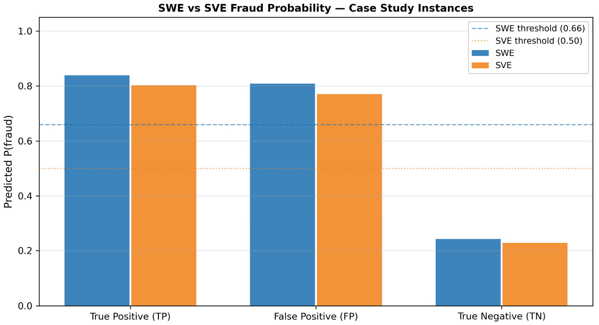
True Negative (Legit)	0.277	0.277	0.130	0.378	0.381	0.240	0.242	LEGIT (both)

presents the complete SWE decision trace for three representative test instances: one correctly identified fraud (true positive), one incorrectly flagged non-fraud case (false positive), and one correctly dismissed legitimate claim (true negative). For each instance, Table 6 shows not only the final prediction but the three-layer decision pathway that produces it: base-model fraud probabilities, SHAP confidence scores, and resulting dynamic weights. Figure 20 summarizes the SWE and SVE probability outputs for each case.

The decision traces in Table 6 reveal several instructive patterns. Most prominently, the SVM weight (w_SVM) varies across instances in a way that the probability outputs alone do not explain. For the true positive and false positive, both high-probability cases, the SVM receives its lowest weight (w = 0.188 and 0.190), reflecting that its SHAP attribution confidence (0.614 and 0.641) is substantially lower than the logistic regression models’ (LR: 1.381 and 1.390, LR_R: 1.391 and 1.403). For the true negative, a low-probability, more uncertain instance, the SVM’s weight rises to 0.240, indicating that the SHAP confidence gap between models narrows when the claim is less obviously fraudulent. This pattern provides a mechanistic insight: the SWE defers more to the margin-based SVM on claims where the feature evidence is ambiguous and more to the logistic regression models on claims where the feature evidence is strong.

The comparison with SVE output (P_SVE) quantifies the practical effect of the dynamic weighting. For the true positive, P_SWE = 0.839 vs. P_SVE = 0.803; for the false positive, P_SWE = 0.808 vs. P_SVE = 0.770; for the true negative, P_SWE = 0.242 vs. P_SVE = 0.228. In all three cases, SWE amplifies the signal relative to SVE; higher fraud probability for the positive cases, lower for the negative because the SHAP weights concentrate voting authority on the models most confident in their feature attributions. At the same optimal threshold, both methods make the same binary decision; the SWE’s advantage is in the calibration of its probability output and the transparency of its decision pathway.

The key interpretability advantage of SWE over SVE is not captured in Figure 20 but in Table 6: for any given claim, an investigator or auditor using SVE can say only that the ensemble predicted fraud with probability 0.803. An investigator using SWE can say the ensemble predicted fraud with probability 0.839; the logistic regression models were the primary contributors (combined weight 0.812) because they identified strong feature signals (SHAP confidence ≈ 1.39 each), while the SVM contributed less (weight 0.188) due to weaker attribution confidence (0.614). This three-layer explanation: which model, how much, and why, is precisely the type of auditable decision pathway that regulatory frameworks such as GDPR Article 22 and the EU AI Act require for automated decisions in high-stakes domains [32,33].

4.12. Synthesis: Positioning SWE as an Interpretability-Driven Architectural Contribution

The empirical results across Section 4.1, Section 4.2, Section 4.3, Section 4.4, Section 4.5, Section 4.6, Section 4.7, Section 4.8, Section 4.9, Section 4.10 and Section 4.11 support three primary conclusions that together define the contribution of the SWE framework.

Competitive performance with transparent aggregation. SWE achieves performance statistically indistinguishable from SVE and AWE across all evaluated metrics; standard and cost-sensitive, default and optimized thresholds, with fully overlapping bootstrap confidence intervals and McNemar p = 1.000. This performance parity is the theoretically expected and mechanistically explained outcome of extreme base-model prediction collinearity (ρ ≥ 0.99, Figure 13). It does not constitute evidence against the framework but constitutes a clearly defined boundary condition for its discriminative impact. The framework’s primary value is not incremental performance over SVE but the transparency of its aggregation mechanism.

Empirical validation of the weighting mechanism. The SWE influence analysis (Section 4.5, Table 5, Figure 10) confirms that SHAP-derived weights are substantially aligned with actual KernelSHAP influence ratios (influence ratios within 5–19% of assigned weights), correcting the 58–380% misalignment observed in the equal-weight diagnostic ensemble (Section 4.4, Figure 8). The dynamic weight distributions (Figure 14) exhibit non-trivial bimodal structure responsive to the explanatory regime of each instance, and the weight–confidence (Figure 15) and weight–disagreement (Figure 16) relationships confirm genuine instance-adaptive behavior. The mechanism works as intended, even when collinearity prevents it from producing measurable performance differentiation.

Architectural interpretability as a first-class property. The case study (Section 4.11, Table 6) demonstrates that SWE provides a three-layer decision trace, base model outputs, SHAP confidence scores, dynamic weights, that is unavailable from standard soft voting and directly addresses regulatory requirements for auditable automated decisions. This is qualitatively different from post hoc SHAP explanations of a fixed-weight ensemble, because the explanation is the mechanism rather than an annotation applied after the fact.

5. Conclusions, Limitations, and Future Directions

This study introduced the SHAP-Weighted Soft Voting Ensemble (SWE), a framework that integrates SHAP attribution magnitudes into the ensemble aggregation process to dynamically weight base-model contributions at the instance level. Empirical evaluation on a publicly available vehicle insurance claims dataset (N = 1000; fraud prevalence 24.7%) with a rigorous statistical evaluation protocol yields four principal findings.

First, SWE achieves performance statistically comparable to equal-weight (SVE) and validation-AUC-weighted (AWE) ensemble baselines, with fully overlapping bootstrap 95% confidence intervals and a McNemar test p-value of 1.000. This performance parity is mechanistically explained by extreme base-model prediction collinearity (ρ ≥ 0.99 among all three SWE base learners) and does not constitute evidence against the framework’s design.

Second, the SHAP influence analysis on the three-model SWE (Section 4.5) demonstrates that SHAP-derived weights are substantially aligned with actual KernelSHAP influence ratios (within 5–19% of assigned weights), validating the core mechanism empirically even in the absence of aggregate performance differentiation.

Third, analysis of the seven-model equal-weight diagnostic ensemble reveals a negative correlation (r = −0.721, p = 0.067, 95% CI [−0.955, 0.070]) between base-model ROC-AUC and ensemble influence; a theoretically coherent but not statistically significant finding at conventional thresholds (n = 7) that motivates further investigation.

Fourth, the global feature importance analysis identifies incident_severity as the dominant predictor across both linear (LR) and tree-based (XGBoost) models, providing convergent validity for this finding and actionable insight for fraud investigators.

5.1. Limitations

Four limitations merit explicit acknowledgement. First, the study relies on a single dataset (N = 1000; fraud prevalence 24.7%), which exceeds the 1–5% prevalence typical of operational insurance portfolios. This difference may influence both model behavior and ensemble diversity, and generalizability to other datasets cannot be assumed.

Second, the restriction to linear base learners, necessary to enable exact LinearSHAP computation, limits the ensemble’s representational flexibility and diversity budget. The L2-norm SHAP confidence measure reflects attribution magnitude rather than calibration accuracy; SHAP magnitude may reflect feature scale or model sensitivity rather than correctness per se. This limitation means that the SWE’s weighting rationale, while structurally principled, is not equivalent to a direct measure of per-instance model reliability.

Third, the calibration analysis reveals that SWE has a slightly higher ECE (0.147) than SVE (0.127), indicating that SHAP-weighted probability aggregation introduces a modest calibration cost. Postprocessing calibration was not applied in this study.

Fourth, the evaluation focuses on predictive performance and architectural interpretability without a human-centered assessment of explanation usefulness. While the SWE framework produces detailed attribution and weighting information at the instance level, its impact on investigator decision making was not directly measured.

5.2. Future Directions

Future research may explore four extensions. First, and most immediately, the integration of heterogeneous base learners, combining LinearSHAP-compatible linear models with TreeExplainer-compatible models, is the highest-priority extension. Under conditions of genuine base-model diversity, the SWE’s SHAP-weighting mechanism is expected to produce measurable performance differentiation alongside enhanced interpretability, directly testing the boundary condition identified in this study.

Second, broader empirical validation across multiple insurance portfolios and additional domains (healthcare fraud, cybersecurity anomaly detection, financial risk assessment) would determine whether the performance–influence paradox and feature importance patterns generalize across datasets with different characteristics and class imbalance ratios.

Third, calibration postprocessing (Platt scaling, temperature scaling, or isotonic regression) applied to SWE outputs may improve probability calibration without altering ranking-level performance, eliminating the trade-off identified in Section 4.9.

Fourth, human-in-the-loop experiments involving fraud investigators would provide empirical evidence regarding the practical utility of the SWE decision trace in real investigative workflows; a necessary step before operational deployment under regulatory scrutiny.

References

1. Harjai, S.; Khatri, S.K.; Singh, G. Detecting Fraudulent Insurance Claims Using Random Forests and Synthetic Minority Oversampling Technique. In Proceedings of the 2019 4th International Conference on Information Systems and Computer Networks (ISCON), Mathura, India, 21–22 November 2019; pp. 123–128. [Google Scholar]
2. Aslam, F.; Hunjra, A.I.; Ftiti, Z.; Louhichi, W.; Shams, T. Insurance fraud detection: Evidence from artificial intelligence and machine learning. Res. Int. Bus. Financ. 2022, 62, 101744. [Google Scholar] [CrossRef]
3. Benedek, B.; Ciumas, C.; Nagy, B.Z. Automobile insurance fraud detection in the age of big data—A systematic and comprehensive literature review. J. Financ. Regul. Compliance 2022, 30, 503–523. [Google Scholar] [CrossRef]
4. Njeru, A.M. Detection of Fraudulent Vehicle Insurance Claims Using Machine Learning; University of Nairobi: Nairobi, Kenya, 2022. [Google Scholar]
5. Mienye, I.D.; Sun, Y. A Survey of Ensemble Learning: Concepts, Algorithms, Applications, and Prospects|IEEE Journals & Magazine|IEEE Xplore. IEEE Access 2022, 10, 99129–99149. [Google Scholar] [CrossRef]
6. Sagi, O.; Rokach, L. Ensemble learning: A survey. Wiley Interdiscip. Rev. Data Min. Knowl. Discov. 2018, 8, e1249. [Google Scholar] [CrossRef]
7. Bourel, M.; Segura, A.M.; Crisci, C.; López, G.; Sampognaro, L.; Vidal, V.; Kruk, C.; Piccini, C.; Perera, G. Machine learning methods for imbalanced data set for prediction of faecal contamination in beach waters. Water Res. 2021, 202, 117450. [Google Scholar] [CrossRef] [PubMed]
8. Khalil, A.A.; Liu, Z.; Fathalla, A.; Ali, A.; Salah, A. Machine Learning Based Method for Insurance Fraud Detection on Class Imbalance Datasets With Missing Values. IEEE Access 2024, 12, 155451–155468. [Google Scholar] [CrossRef]
9. Dhieb, N.; Ghazzai, H.; Besbes, H.; Massoud, Y. A Secure AI-Driven Architecture for Automated Insurance Systems: Fraud Detection and Risk Measurement. IEEE Access 2020, 8, 58546–58558. [Google Scholar] [CrossRef]
10. Liu, S.; Andrienko, G.; Wu, Y.; Cao, N.; Jiang, L.; Shi, C.; Wang, Y.-S.; Hong, S. Steering data quality with visual analytics: The complexity challenge. Vis. Inform. 2018, 2, 191–197. [Google Scholar] [CrossRef]
11. Viaene, S.; Derrig, R.A.; Baesens, B.; Dedene, G. A Comparison of State-of-the-Art Classification Techniques for Expert Automobile Insurance Claim Fraud Detection. J. Risk Insur. 2002, 69, 373–421. [Google Scholar] [CrossRef]
12. Dhieb, N.; Ghazzai, H.; Besbes, H.; Massoud, Y. Extreme Gradient Boosting Machine Learning Algorithm For Safe Auto Insurance Operations. In Proceedings of the 2019 IEEE International Conference on Vehicular Electronics and Safety (ICVES), Cairo, Egypt, 4–6 September 2019; pp. 1–5. [Google Scholar]
13. Itri, B.; Mohamed, Y.; Mohammed, Q.; Omar, B. Performance comparative study of machine learning algorithms for automobile insurance fraud detection. In Proceedings of the 2019 Third International Conference on Intelligent Computing in Data Sciences (ICDS), Marrakech, Morocco, 28–30 October 2019; pp. 1–4. [Google Scholar]
14. Hanafy, M.; Ming, R. Using machine learning models to compare various resampling methods in predicting insurance fraud. J. Theor. Appl. Inf. Technol. 2021, 99, 2819–2833. [Google Scholar]
15. Komsrimorakot, P.; Siriborvornratanakul, T. Enhancing fraud detection in imbalanced motor insurance datasets using CP-SMOTE and Random Under-Sampling. J. Big Data 2025, 12, 172. [Google Scholar] [CrossRef]
16. Nordin, S.-Z.S.; Wah, Y.B.; Haur, N.K.; Hashim, A.; Rambeli, N.; Jalil, N.A. Predicting automobile insurance fraud using classical and machine learning models. Int. J. Electr. Comput. Eng. (IJECE) 2024, 14, 911–921. [Google Scholar] [CrossRef]
17. Kini, A.; Chelluru, R.; Naik, K.; Naik, D.; Aswale, S.; Shetgaonkar, P. Automobile insurance fraud detection: An overview. In Proceedings of the 2022 3rd International Conference on Intelligent Engineering and Management (ICIEM), London, UK, 27–29 April 2022; pp. 7–12. [Google Scholar]
18. Khan, A.; Dhungana, K.; Gyawali, S.; Sharma, I. Forecasting Automobile Insurance Claims: Examining the Interplay of Policyholder Traits for Enhanced Predictive Insights. In Proceedings of the 2024 2nd International Conference on Intelligent Data Communication Technologies and Internet of Things (IDCIoT), Bengaluru, India, 4–6 January 2024; pp. 881–886. [Google Scholar]
19. Davis, J.; Goadrich, M. The relationship between Precision-Recall and ROC curves. In Proceedings of the 23rd International Conference on Machine Learning, Pittsburgh, PA, USA, 25–29 June 2006; pp. 233–240. [Google Scholar]
20. Saito, T.; Rehmsmeier, M. The Precision-Recall Plot Is More Informative than the ROC Plot When Evaluating Binary Classifiers on Imbalanced Datasets. PLoS ONE 2015, 10, e0118432. [Google Scholar] [CrossRef] [PubMed]
21. Vorobyev, I. Fraud risk assessment in car insurance using claims graph features in machine learning. Expert Syst. Appl. 2024, 251, 124109. [Google Scholar] [CrossRef]
22. Mokgwatjane, K.; Paepae, T. An explainable ensemble machine learning approach for multi-domain, multiclass sentiment analysis in Amazon product reviews. Mach. Learn. Appl. 2026, 23, 100825. [Google Scholar] [CrossRef]
23. Ngwenya, B.; Paepae, T.; Bokoro, P.N. Advancing SDG 6.3. 2 with machine learning-based virtual sensors for high-frequency nutrient monitoring. J. Water Process Eng. 2025, 79, 108831. [Google Scholar] [CrossRef]
24. Teffo, N.; Bokoro, P.; Muremi, L.; Paepae, T. Performance evaluation of selected machine learning techniques in the detection of non-technical losses in the distribution system. In Proceedings of the 2024 32nd Southern African Universities Power Engineering Conference (SAUPEC), Stellenbosch, South Africa, 24–25 January 2024; pp. 1–5. [Google Scholar]
25. Ding, Y.; Zhu, H.; Chen, R.; Li, R. An Efficient AdaBoost Algorithm with the Multiple Thresholds Classification. Appl. Sci. 2022, 12, 5872. [Google Scholar] [CrossRef]
26. General Data Protection Regulation. Art. 22 GDPR. Automated Individual Decision-Making, Including Profiling. Intersoft Consulting 2020. Available online: https://gdpr-info.eu/art-22-gdpr (accessed on 19 March 2026).
27. EUAI Act. The eu Artificial Intelligence Act; European Union: Brussels, Belgium, 2024; Available online: https://artificialintelligenceact.eu/ (accessed on 19 March 2026).
28. Lundberg, S.M.; Lee, S.-I. A unified approach to interpreting model predictions. Adv. Neural Inf. Process. Syst. 2017, 30, 4768–4777. Available online: https://dl.acm.org/doi/10.5555/3295222.3295230 (accessed on 19 March 2026).
29. Debener, J.; Heinke, V.; Kriebel, J. Detecting insurance fraud using supervised and unsupervised machine learning. J. Risk Insur. 2023, 90, 743–768. [Google Scholar] [CrossRef]
30. ABDELRAHIM AQQAD. Insurance_Claims. Mendeley Data. 2023. Available online: https://data.mendeley.com/datasets/992mh7dk9y/2 (accessed on 19 March 2026).
31. Akiba, T.; Sano, S.; Yanase, T.; Ohta, T.; Koyama, M. Optuna: A next-generation hyperparameter optimization framework. In Proceedings of the 25th ACM SIGKDD International Conference on Knowledge Discovery & Data Mining, New York, NY, USA, 4–8 August 2019; pp. 2623–2631. [Google Scholar]
32. Hamon, R.; Junklewitz, H.; Sanchez, I.; Malgieri, G.; De Hert, P. Bridging the gap between AI and explainability in the GDPR: Towards trustworthiness-by-design in automated decision-making. IEEE Comput. Intell. Mag. 2022, 17, 72–85. [Google Scholar] [CrossRef]
33. Damen, V.; Wiersma, M.; Aydin, G.; van Haasteren, R. Explainable AI for EU AI Act compliance audits. Maandbl. Voor Account. En Bedrijfsecon. 2025, 99, 231–242. [Google Scholar] [CrossRef]
Figure 1. Workflow of the proposed SHAP-weighted soft voting ensemble framework for interpretable vehicle insurance fraud detection.
Information 17 00607 g001
Figure 2. Conceptual motivation for the SHAP-weighted soft voting ensemble. Traditional soft voting assigns equal weights to all models regardless of their predictive influence. The proposed method derives weights from SHAP-based influence scores, allowing models with stronger explanatory contributions to exert greater influence on the ensemble decision.
Information 17 00607 g002
Figure 3. Five-fold cross-validation ROC-AUC distributions for all eight base learners. Boxes represent interquartile ranges; whiskers extend to ±1.5 × IQR; horizontal bars indicate median values.
Information 17 00607 g003
Figure 4. ROC curves (left) and Precision–Recall curves (right) for all models on the held-out test set.
Information 17 00607 g004
Figure 5. Multi-metric comparison bar chart (ROC-AUC, PR-AUC, F1, Recall, Precision) for all models at the default threshold = 0.5.
Information 17 00607 g005
Figure 6. Ablation study: weighting strategy comparison across SVE, SWE, and AWE on ROC-AUC, PR-AUC, F1, Recall, and Precision. Annotated values confirm metric-level parity across all three strategies.
Information 17 00607 g006
Figure 7. Performance–Influence Paradox: 7-Model Diagnostic Ensemble. Scatter plot of base-model ROC-AUC vs. normalized SHAP influence. AdaBoost (bottom right) combines the highest individual ROC-AUC with the lowest ensemble influence.
Information 17 00607 g007
Figure 8. Voting Weight vs. Actual SHAP Influence: 7-Model Diagnostic Ensemble. All seven models share the same assigned weight (0.143) yet span a 3.8-fold range of actual influence (0.060–0.228). Divergence from the perfect-alignment diagonal quantifies the misalignment that equal-weight voting introduces.
Information 17 00607 g008
Figure 9. SHAP-Based Model Influence Analysis: 3-Model SWE. Left panel: absolute influence (Mean |SHAP|) showing LR and LR_R with near-identical importance and SVM with lower influence. Right panel: directional influence (Mean SHAP) revealing that LR exerts a net negative directional pull (reducing fraud probability relative to the ensemble mean) while LR_R and SVM exert positive directional influence.
Information 17 00607 g009
Figure 10. Voting Weight vs. Actual SHAP Influence: 3-Model SWE. All three models lie close to the perfect-alignment diagonal, contrasting sharply with the severe misalignment visible in Figure 8 for the equal-weight diagnostic ensemble. This alignment validates that the SWE’s SHAP-derived weights successfully calibrate voting authority to actual model influence at the instance level.
Information 17 00607 g010
Figure 11. Global Feature Importance: LR Coefficients (SHAP Proxy). Feature importances aggregated across one-hot encoded subcategories, revealing incident_severity as the dominant predictor with a coefficient magnitude 4.4× larger than the second-ranked feature.
Information 17 00607 g011
Figure 12. Global Feature Importance: XGBoost (TreeSHAP beeswarm plot). Each point represents one test instance. Color encodes feature value (red = high, blue = low). The horizontal spread shows SHAP impact on fraud probability. incident_severity_Major Damage dominates, with a clear bimodal pattern: absent instances cluster near zero while present instances show strongly positive SHAP values.
Information 17 00607 g012
Figure 13. Correlation Between Base-Model Prediction Probabilities: 7-model diagnostic ensemble. All pairwise correlations among the three SWE base learners (LR, LR_R, SVM) exceed ρ = 0.99, with LR–LR_R achieving ρ = 1.00. This extreme collinearity mechanistically explains why no weighting scheme can produce different aggregate predictions.
Information 17 00607 g013
Figure 14. Distributions of dynamically assigned SHAP-based voting weights across 200 test instances for each SWE base model. Both LR and LR_R exhibit bimodal distributions with peaks near 0.37–0.38 and 0.42–0.43, while SVM is right-skewed with a dominant peak near 0.19–0.20, indicating that the mechanism adapts to two distinct explanatory regimes.
Information 17 00607 g014
Figure 15. Dynamic Model Weights vs. Prediction Confidence (SWE output probability). The non-flat, structured relationship across all three models confirms that SWE performs instance-adaptive reweighting rather than static averaging; the weights respond to the ensemble’s level of prediction confidence for each claim.
Information 17 00607 g015
Figure 16. SWE Weight Allocation vs. Model Disagreement (standard deviation of base-model probability outputs). Increased weight spread at higher disagreement levels confirms that the SWE mechanism is more discriminating in uncertain regions of the feature space, the exact property motivating adaptive ensemble weighting.
Information 17 00607 g016
Figure 17. Decision Threshold Sensitivity Analysis for SWE (left), SVE (center), and AWE (right). F1-score, Precision, and Recall are plotted across thresholds from 0.05 to 0.95. F1-optimal thresholds (dashed vertical lines) are SWE = 0.660, SVE = 0.625, AWE = 0.625. The broad F1 plateau from 0.45–0.75 indicates robustness to threshold choice within this range.
Information 17 00607 g017
Figure 18. Reliability Diagrams (calibration curves) with expected calibration error (ECE) for SWE (0.147), SVE (0.127), AWE (0.127), LR (0.186), and RF (0.187). Ensemble methods outperform individual models in calibration; SWE’s slightly elevated ECE reveals a calibration trade-off introduced by SHAP-weighted aggregation.
Information 17 00607 g018
Figure 19. Cost-Sensitive Evaluation at Cost-Optimal Threshold (FN cost = 10×, FP cost = 1×). All three ensemble variants achieve identical total cost of 151 at the cost-optimal threshold of 0.05. The shared cost reflects both the prediction-level identity confirmed by McNemar’s test and the asymmetric cost structure that drives optimal thresholds toward aggressive recall.
Information 17 00607 g019
Figure 20. SWE vs. SVE Fraud Probability: Case Study Instances. Grouped bar chart comparing P_SWE and P_SVE for the True Positive, False Positive, and True Negative instances from Table 6. Model-specific optimal thresholds are shown as horizontal reference lines.
Information 17 00607 g020