Leveraging Feature Selection and Ensemble Learning to Predict Secondary School Achievement: A Comparative Study of Three Grade Granularities

Abstract

Predictive analytics has become increasingly important in educational decision-making, supporting at-risk identification and adaptive tutoring. The accurate early prediction of school achievement can enable timely intervention. Using the Math Students dataset, which contains data on students from two Portuguese secondary schools, we model three categorical outcomes derived from the students’ final grade, namely the final grade level (low, medium, high), its qualitative evaluation (fail, satisfactory, good, excellent), and the final pass/fail outcome. After preprocessing, three filter methods—Correlation-Based Feature Subset Selection (CFS), Correlation Attribute Evaluation (CorrEval), and Information Gain (InfoGain)—are applied to reduce the dimensionality of the datasets. Nine classifiers (Naive Bayes, Logistic, MLP, SMO, IBk, Bagging, J48, Random Forest, Random Tree) are evaluated using ten-fold cross-validation in the Waikato Environment for Knowledge Analysis (Weka) platform. Random Forest with InfoGain achieves 90.7% accuracy on the three-band task, while Bagging with InfoGain achieves 92.5% on the binary pass/fail outcome, outperforming benchmarks in prior Educational Data Mining (EDM) studies. Results confirm that prior academic performance indicators (first- and second-period grades) and failure history dominate predictive power and contribute substantially to the success of ensemble models, particularly when paired with feature selection methods that reduce noise and highlight relevant attributes.

1. Introduction

Predictive analytics plays a pivotal role in educational decision-making by facilitating the early identification of at-risk students and supporting the design of adaptive tutoring interventions [1]. By analyzing historical and real-time data, such as student demographics, academic performance, engagement patterns, and behavioral indicators, predictive analytics aims to estimate the likelihood of events such as academic success, failure, dropout, or course completion, supporting the design of targeted interventions, the personalization of learning pathways, and the efficient allocation of educational resources. Romero and Ventura [2] emphasized the central role of predictive models in shaping learning analytics interventions, while systematic reviews [3,4] confirmed the growing reliance on AI-driven methods in the field. Recent advances have focused not only on improving predictive accuracy, but also on ensuring transparency, interpretability, and fairness, for example through interpretable models that allow educators to understand the drivers of predictions [5,6]. These studies collectively underline the importance of both methodological rigor and practical applicability in deploying predictive analytics for educational decision-making.

Machine learning (ML) techniques have been extensively adopted in educational decision-making to model, predict, and explain student learning outcomes. Supervised learning algorithms such as Logistic Regression, Naive Bayes, Support Vector Machines, k-Nearest Neighbors, and Artificial Neural Networks are frequently employed to predict academic performance, course completion, and dropout risk [7,8]. Ensemble learning has been widely explored as a means of improving the accuracy of educational outcome prediction. Random Forest and boosting approaches, in particular, have consistently outperformed single classifiers in predicting pass/fail status or grade categories [7,9]. These ensemble methods are especially valued for their ability to capture nonlinear relationships and achieve comparatively high predictive accuracy across diverse educational datasets [2,10]. Recent work has further refined ensemble frameworks by incorporating optimization procedures such as particle swarm optimization and adaptive weighting to enhance predictive performance on imbalanced datasets [11]. Similarly, Tong and Li [6] demonstrated that stacking ensembles combined with explainable AI procedures could provide both high accuracy and interpretability when forecasting student achievement, thereby highlighting the practical value of ensemble approaches. More recently, deep learning tools have been explored in large-scale and online learning environments, especially for modeling sequential and temporal data such as clickstream logs and features for early warning systems of student success [12,13]. Across these studies, ML models support educators in identifying at-risk students, personalizing instruction, and informing evidence-based interventions.

Feature selection is a critical step in developing robust and efficient ML models, as it enhances interpretability, reduces dimensionality, and mitigates overfitting risks [14]. Approaches are typically categorized into filter, wrapper, and embedded methods. Filter algorithms, such as Information Gain or correlation-based criteria, rank attributes independently of the learning algorithm. Wrapper techniques evaluate subsets of features by training a predictive model, while embedded strategies incorporate selection during training, as in LASSO (Least Absolute Shrinkage and Selection Operator) regularization [15,16]. Filter-based tools have been shown to reduce noise and improve both the interpretability and model performance of models in educational data mining [2,14,15]. More recent work has extended this line of research by proposing hybrid or ensemble-based feature selection approaches that combine multiple criteria to identify stable sets of predictive features [17,18]. In prior studies, past academic performance (e.g., first- and second-period grades), prior failures, and behavioral variables such as absences consistently emerge as dominant predictors, corroborating the findings of earlier benchmark studies.

Despite the substantial progress achieved by ML and ensemble-based methodologies in predicting educational outcomes, important challenges remain that limit their practical adoption and generalizability. In particular, predictive models must remain interpretable to practitioners to support trust, transparency, and informed pedagogical decision-making [19]. At the same time, models should generalize robustly across different grading schemes and outcome definitions, as educational performance may be represented using binary pass/fail labels, ordinal grade bands, or finer-grained categorical evaluations [20]. Addressing these challenges is especially important in secondary education settings, where predictive systems are expected to support early intervention, while remaining adaptable to diverse assessment frameworks. These considerations motivate the investigation of ensemble learning in combination with feature selection across multiple grade granularities, enabling a more comprehensive evaluation of model performance.

Building upon the foundational study of Cortez and Silva [21], who first applied data mining techniques to the Portuguese secondary school student dataset and established it as a benchmark in educational data mining, this work investigates the predictive modeling of student achievement from a comparative and multi-granular perspective. While prior studies demonstrated that decision trees, random forests, and neural networks can predict student grades with moderate accuracy, emphasizing the dominant role of past academic performance and socio-economic factors, most evaluations have been limited to a single outcome definition. Extending this seminal work, we derive three categorical representations of the final grade, corresponding to distinct levels of granularity, and systematically evaluate nine classification algorithms under three widely used filter-based feature selection paradigms. Comparative analyses of such strategies remain relatively scarce in the educational domain; existing surveys review techniques in isolation but do not examine their behavior across multiple grading schemes. To address this gap, our study employs the three most frequently cited filter methods in combination with both interpretable learners, such as J48 [22], and state-of-the-art ensemble models. This experimental design enables a comprehensive assessment of how feature selection and ensemble learning interact across different grade granularities, providing insights into the trade-offs between predictive accuracy, interpretability, and robustness.

In this context, the present study provides a unified and systematic comparison of student performance prediction under different outcome representations. By considering three alternative formulations of the target variable, the analysis highlights how the level of granularity influences model behavior and predictive efficiency. At the same time, the study examines the role of widely used filter-based feature selection approaches within a consistent experimental framework, allowing their relative effectiveness to be assessed across different prediction settings. In addition, a broad set of ML algorithms is evaluated under uniform conditions, enabling a transparent comparison of their performance and supporting reproducibility. Particular attention is also given to an early prediction setting, where prior academic indicators are excluded, in order to explore the practical potential of timely intervention. Finally, the inclusion of robustness analyses provides additional confidence that the reported results are not driven by specific preprocessing or modeling choices. Taken together, these elements provide a more comprehensive perspective on student performance prediction and extend existing work by jointly examining outcome definition, feature selection, and model behavior within a single experimental framework.

2. Materials and Methods

2.1. Data Description

The Math Students Dataset contains data on 395 students from two Portuguese secondary schools (Gabriel Pereira and Mousinho da Silveira). It includes 33 attributes covering demographic, educational, behavioral, and lifestyle-related variables. These attributes provide a comprehensive set of predictors for modeling students’ final academic performance. Demographic variables describe the student’s background, such as school attended, gender, age, home address type, family size, and parental cohabitation status. Socio-economic indicators capture parental education levels and occupations, the reason for school choice, and the student’s primary guardian. Academic and school-related factors include travel time to school, weekly study time, number of past academic failures, attendance in nursery school, participation in extracurricular activities, access to educational support (school-based, family-based, or paid classes), and aspirations for higher education. Behavioral and lifestyle variables reflect family relationships, leisure time, social activities, alcohol consumption during weekdays and weekends, health status, and the number of school absences. Academic performance is represented through grades from the first and second grading periods (G1 and G2), as well as the final grade (G3).

Table 1. Description of variables in the Portuguese mathematics students’ dataset.

Variable	Description
school	Student’s school (‘GP’—Gabriel Pereira or ‘MS’—Mousinho da Silveira)
sex	Student’s sex (‘F’—female or ‘M’—male)
age	Student’s age (15 to 22)
address	Home address type (‘U’—urban or ‘R’—rural)
famsize	Family size (‘LE3’—less than or equal to 3 or ‘GT3’—greater than 3)
pstatus	Parent’s cohabitation status (‘T’—together or ‘A’—apart)
medu	Mother’s education (0 to 4)
fedu	Father’s education (0 to 4)
mjob	Mother’s job (‘teacher’, ‘health’, ‘services’, ‘at_home’, ‘other’)
fjob	Father’s job (‘teacher’, ‘health’, ‘services’, ‘at_home’, ‘other’)
reason	Reason for choosing the school (‘home’, ‘reputation’, ‘course’, ‘other’)
guardian	Student’s guardian (‘mother’, ‘father’, ‘other’)
traveltime	Travel time to school (1 to 4)
studytime	Weekly study time (1 to 4)
failures	Number of past class failures (numeric)
schoolsup	Extra educational support (yes or no)
famsup	Family educational support (yes or no)
paid	Extra paid classes within the course (yes or no)
activities	Extracurricular activities (yes or no)
nursery	Attended nursery school (yes or no)
higher	Aspires to higher education (yes or no)
internet	Internet access at home (yes or no)
romantic	In a romantic relationship (yes or no)
famrel	Family relationship quality (1 to 5)
freetime	Free time after school (1 to 5)
goout	Going out with friends (1 to 5)
dalc	Weekday alcohol consumption (1 to 5)
walc	Weekend alcohol consumption (1 to 5)
health	Current health status (1 to 5)
absences	Number of school absences (0 to 93)
G1	First-period grade (0 to 20)
G2	Second-period grade (0 to 20)
G3	Final (third-period) grade (0 to 20)

presents a detailed description of the variables contained in the Portuguese mathematics students’ dataset.

The dataset reflects the Portuguese secondary education system, which uses a 0–20 grading scale and socio-economic and school-level characteristics as defined in the Portuguese secondary education system. Factors such as parental occupation categories, educational support structures, and school choice motivations are defined according to Portuguese educational practices. Therefore, while the modeling framework is methodologically general, the interpretation of specific predictors should be considered within this educational and socio-economic setting.

The primary objective of this study is to classify the students’ final grades (G3) into different categories based on a set of independent variables. These categories are split into three different dependent variables: (a) the final grade level (ordinal performance levels), (b) the final grade categorization, and (c) the pass/fail distinction (binary outcome). The final grade level (G3_level) categorizes students into low (G3 < 10), medium (10 ≤ G3 < 15), or high (G3 ≥ 15) performance groups based on thresholds in G3. The thresholds were set based on the data distribution and the needs of educational analysis. The final grade categorization (G3_grade) is a more detailed classification of students’ final grades, distinguishing between fail (G3 < 10), satisfactory (10 ≤ G3 < 13), good (13 ≤ G3 < 15), and excellent (G3 ≥ 15) performance. This formulation enables a more nuanced assessment of students’ academic achievement. The pass/fail binary classification represents whether a student passed (G3 ≥ 10) or failed (G3 < 10) based on G3. This binary representation provides a simplified distinction between successful and unsuccessful academic outcomes, which is useful for basic educational interventions. For the binary G3_pass/fail outcome, 66.3% of students were classified as passing and 33.7% as failing, indicating a moderately balanced class distribution.

2.2. Data Preprocessing

The data are originally in raw format and therefore require preprocessing before ML algorithms can be applied. The preprocessing steps include handling missing values, encoding categorical data, normalizing continuous attributes, and splitting the dataset into training and testing sets for cross-validation.

In educational datasets, missing values constitute a common challenge arising from incomplete survey responses, data entry errors, or unreported information. In this study, missing data were primarily observed in attributes related to family educational support, student participation in extracurricular activities, and self-reported health status. To address this issue, a simple and widely adopted imputation strategy was applied. Specifically, continuous variables (e.g., health index scores and other numeric indicators) were imputed using the arithmetic mean of the observed (non-missing) values, whereas categorical variables (e.g., participation status and types of family support) were imputed using the mode, defined as the most frequently occurring category. Mean/mode imputation is commonly employed due to its simplicity, interpretability, and low computational cost, and is frequently used as a baseline approach in applied ML studies [23,24]. This strategy ensures that no instances are discarded, thereby preserving the sample size for model training and enabling consistent comparison across different grade granularities. However, mean/mode imputation relies on strong assumptions regarding the missingness mechanism, typically that data are missing completely at random, and is known to underestimate variance by concentrating imputed values around measures of central tendency. As documented in the literature, this can distort inter-variable relationships, bias parameter estimates, and attenuate correlations, particularly when missingness is systematic rather than random [25]. More sophisticated imputation techniques were deliberately avoided in this work to maintain methodological consistency and fairness across classifiers, as such techniques may implicitly favor distance-based or model-specific learners and introduce additional sources of variance into the comparative evaluation.

Machine learning algorithms generally require numerical input, which necessitates the transformation of categorical attributes into a suitable numeric representation. In this study, several variables, such as sex, school, and participation in extracurricular activities, were categorical and therefore required preprocessing before model training. To achieve this, one-hot encoding was employed, a widely adopted technique that converts each value into a set of binary indicator variables. Each new column represents one category, with values of 1 indicating presence and 0 indicating absence. For example, the attribute school, which originally consisted of two categories (school A and B), was transformed into two distinct binary columns. Similarly, the attribute sex was encoded into binary indicator variables, male and female. One-hot encoding has the advantage of preserving categorical distinctions without imposing ordinal assumptions that might otherwise distort the data [26].

While one-hot encoding is among the most widely used techniques for handling categorical variables, alternative strategies include label encoding, target encoding, and embedding-based representations. In the present study, one-hot encoding was selected for several reasons. First, the categorical variables exhibit relatively low cardinality, thereby limiting feature space inflation and mitigating sparsity-related concerns [27]. Second, the ensemble learning techniques employed, such as Random Forests, are well suited to handling sparse binary features and have been shown to perform robustly under such representations [2]. Third, this method preserves transparency and interpretability within the preprocessing pipeline, enabling clear attribution of predictive effects to individual categories and reducing the risk of information leakage that may arise with target-based encoding methods [28]. Taken together, these considerations support the use of one-hot encoding over more complex alternatives.

Continuous attributes in the dataset, such as age, study time, and prior academic performance (G1 and G2), were normalized to the fixed range [0,1] using min–max scaling. Normalization represents a fundamental preprocessing step for ML algorithms that rely on distance-based measures or optimization procedures sensitive to feature magnitude. In particular, algorithms such as Support Vector Machines (SVM) and k-Nearest Neighbors (k-NN) may be disproportionately influenced by variables with larger numerical ranges, resulting in biased distance computations or distorted decision boundaries [29]. By rescaling all continuous features to a common range, min–max normalization ensures that each attribute contributes proportionally to the learning process, thereby improving numerical stability and supporting fair comparison across features. To mitigate the risk of data leakage, normalization was applied within the cross-validation procedure, following standard ML practice.

To obtain an unbiased and reliable estimate of model performance, ten-fold cross-validation was employed, which is a well-established ML resampling strategy. Under this procedure, the dataset was randomly partitioned into ten mutually exclusive subsets (folds) of approximately equal size. In each iteration, one fold was held out as the test set, while the remaining nine were used for training. This process was repeated ten times so that each instance was used exactly once for testing and nine times for training. The use of this approach offers two key advantages: first, it maximizes the effective use of limited data by allowing all observations to contribute to both model training and evaluation; second, it reduces the risk of biased performance estimates that may arise from a single train–test split. Compared to simple hold-out validation, cross-validation has been shown to provide more robust and generalizable estimates of prediction reliability, particularly for datasets of moderate size [30,31]. The use of stratified ten-fold cross-validation provides a robust internal estimate of model performance while maintaining class distribution consistency across folds. However, it should be noted that it evaluates internal generalization within the same dataset rather than external generalization across different educational contexts. After completing the procedure, evaluation metrics such as accuracy, F1-score, and area under the receiver operating characteristic curve (AUC) were averaged [32] across the ten folds to yield a stable overall performance estimate. This averaging process reduces variability arising from random partitioning and mitigates the risk of overfitting to a particular subset of the data. Model evaluation was primarily based on overall classification accuracy, which provides an intuitive measure of the proportion of correctly classified instances across all classes. In addition, class-wise precision, recall, and F1-scores were computed to assess the predictive robustness for individual classes, while the macro-averaged AUC was calculated to evaluate the models’ discriminative capability independent of class imbalance. Furthermore, confusion matrices were analyzed to identify common misclassification patterns and to provide additional insight into the types of classification errors produced by the models.

2.3. Feature Selection

Feature selection is a critical stage in the ML pipeline, particularly when working with educational datasets that may include numerous demographic, behavioral, and academic variables. Its main objective is to identify and retain the most informative attributes while eliminating redundant or irrelevant ones. This process not only improves predictive capability by reducing noise in the data, but also enhances model interpretability and mitigates the risk of overfitting [33]. Moreover, feature selection contributes to computational efficiency, which becomes increasingly important when experimenting with multiple algorithms and parameter settings. Three feature selection methods were applied to this dataset: (i) Correlation-Based Feature Subset Selection (CFS), (ii) Correlation Attribute Evaluation (CorrEval), and (iii) Information Gain (InfoGain).

The CFS method evaluates subsets of features rather than individual variables. It selects groups of features that are highly correlated with the target variable while being minimally correlated with each other. The underlying assumption is that effective feature subsets contain attributes that are strongly predictive individually and weakly redundant collectively [15]. CFS has been widely used in educational data mining to identify meaningful predictors of student achievement, as it naturally highlights both academic and non-academic attributes that contribute to learning outcomes [2]. By focusing on correlations, it provides interpretable results that align with theoretical expectations, making it suitable for comparative studies across multiple predictive tasks. In this study, the CFS method was applied separately to each of the three dependent variables under investigation, namely ordinal performance levels, four-level grade categories, and the binary pass/fail outcome.

The CorrEval method computes the correlation between each feature and the target variable independently. Features with stronger correlation values (positive or negative) are ranked higher, reflecting their predictive contribution. Unlike CFS, which evaluates subsets, this approach focuses on the direct linear relationship between each variable and the outcome [34]. This process is particularly efficient for high-dimensional datasets, as it provides a simple and interpretable metric for feature relevance without the need for iterative search procedures. In this study, the method was applied separately to each of the three dependent variables. CorrEval is valued for its simplicity, transparency, and computational efficiency, making it suitable as a first step in feature analysis. However, its reliance on pairwise linear associations introduces several limitations. The method does not account for redundancy among correlated variables, nor does it capture nonlinear relationships unless they manifest as strong monotonic correlations.

InfoGain quantifies the reduction in entropy achieved by partitioning a dataset according to a given feature. Rooted in information theory, InfoGain measures the reduction in uncertainty about the target variable provided by knowing the value of a feature [35]. Independent variables that yield larger entropy reductions are therefore considered more informative and prioritized for selection. InfoGain is particularly effective in classification tasks, as it identifies attributes with strong discriminative power, even when the underlying relationships are not strictly linear. By explicitly modeling uncertainty reduction, this method is able to capture predictive relevance arising from complex, nonlinear associations. Despite its advantages, it exhibits several well-documented limitations. Most notably, it is biased toward features with a large number of distinct values, such as categorical attributes with many levels. Furthermore, it evaluates each feature independently, ignoring interactions and redundancy, which may result in selecting correlated attributes [14,15]. These limitations motivate the complementary use of correlation-based or subset-based feature selection methods in comparative experimental designs.

While the CorrEval method highlights features with strong direct associations, it may overlook features whose predictive value emerges through interactions with other variables. This contrasts with the CFS method, which explicitly accounts for feature redundancy, and the InfoGain approach, which detects information-theoretic contributions beyond linear correlations. Taken together, these differences underscore the complementary value of applying multiple feature selection techniques in parallel: while CorrEval identifies the most individually powerful predictors, methods like CFS and InfoGain broaden the analysis by capturing subsets or nonlinear associations.

Feature selection was conducted using parameter settings that reflect widely adopted best-practice defaults reported in the literature. Specifically, the CFS method employed a BestFirst search strategy to identify compact, non-redundant subsets, while CorrEval retained attributes exceeding a correlation threshold of r > 0.10. InfoGain ranking was applied using a minimum threshold of IG > 0.02 to filter out features with negligible information-theoretic contribution. Such threshold-based filtering and search configurations are widely recommended to balance sensitivity to informative features against the risk of noise amplification and over-selection [14,36]. Collectively, these configurations ensure methodological consistency across outcome granularities and facilitate a fair comparison of feature selection strategies within the proposed framework.

2.4. Machine Learning Algorithms

To comprehensively evaluate model performance across different grade granularities, a diverse suite of ML classifiers is applied, encompassing probabilistic, linear, neural, instance-based, tree-based, and ensemble methods. This diversity enables both the comparison simpler, more interpretable models against more complex ones, but also to test how each algorithm interacts with the feature selection and preprocessing pipeline. Many educational data mining studies have found that no single method uniformly dominates across datasets, making a comparative approach essential [37].

Naive Bayes is a probabilistic classification algorithm based on Bayes’ theorem, assuming conditional independence among predictors. Despite its simplifying independence assumption, it showed competitive performance in many real-world applications, particularly in domains characterized by noisy, high-dimensional, and heterogeneous data. Its computational efficiency, low training cost, and robustness to irrelevant features make it a popular baseline classifier. Previous studies have shown that Naive Bayes can maintain stable predictive performance even when the independence assumption is violated, as probability estimates may still yield accurate class rankings [38,39]. In educational datasets, it has been applied to tasks such as predicting academic progress or dropout risk (e.g., Monteverde-Suárez et al. [40]). Although it is often outperformed by ensemble models in terms of absolute accuracy, it remains a useful and interpretable benchmark, especially when combined with feature selection techniques that reduce redundancy and noise [14].

Logistic Regression is a widely used linear classifier that estimates the probability of class membership through a logistic (sigmoid) function applied to a linear combination of input features. Due to its simplicity, statistical grounding, and probabilistic output, it is frequently employed as a strong baseline in predictive modeling tasks. Its coefficients provide direct insight into the direction and magnitude of each predictor’s influence, making it highly interpretable and suitable for educational decision-making contexts. Despite assuming linear relationships, Logistic Regression has demonstrated competitive performance in student performance and dropout prediction tasks, particularly when relevant features are carefully selected and multicollinearity is controlled [10,41]. It is widely adopted in educational data mining for its robustness, ease of implementation, and ability to generalize across datasets with varying class distributions [2,42].

Multilayer Perceptron (MLP) neural networks are feedforward models consisting of input, hidden, and output layers, where nonlinear activation functions enable the modeling of complex relationships among features. Trained through backpropagation, MLPs adjust connection weights iteratively to minimize prediction error and capture nonlinear interactions that cannot be represented by linear models. In educational data mining, MLPs have been used to predict student achievement, dropout risk, and learning outcomes, particularly when relationships between academic, behavioral, and socio-demographic variables are complex [2,43]. Empirical studies suggest that MLPs can outperform simpler classifiers when sufficient data and appropriate regularization are available, although they are more sensitive to parameter tuning and feature scaling [30,41]. Despite their strong representational capacity, their limited interpretability compared to simpler models remains a consideration in educational decision-making contexts [2,43].

Support Vector Machines (SVMs) are margin-based classifiers that construct an optimal separating hyperplane by maximizing the margin between classes. Through the use of kernel functions, they can model nonlinear decision boundaries while maintaining strong generalization performance. SVM training is formulated as a convex quadratic optimization problem, for which efficient decomposition-based solvers, such as those implemented in Sequential Minimal Optimization (SMO)-style algorithms, enable scalable learning on medium-sized datasets [44,45]. SVMs have been widely applied in educational data mining for tasks such as student performance and dropout prediction, often achieving competitive accuracy compared to neural and ensemble models [7,8]. Their effectiveness in high-dimensional settings is well documented, although performance is sensitive to kernel choice and hyperparameter tuning [2,41,46,47]. Despite their strong predictive capability, their limited interpretability compared to simpler models remains a consideration in educational applications.

Instance-based learning, represented in this study by the k-Nearest Neighbors (k-NN, IBk) algorithm, classifies new instances based on the labels of the most similar training examples using a distance metric. In educational data mining, k-NN has been applied to tasks such as student performance and dropout prediction, particularly when relationships between variables are complex and nonlinear [2,8]. Its performance depends on the choice of neighborhood size, distance metric, and feature scaling [10,41]. In this study, k was set to 5, a commonly adopted value that balances sensitivity to local patterns with robustness to noise. While k-NN can achieve competitive accuracy, its computational cost at prediction time and limited interpretability compared to other models may restrict its use in large-scale applications. Nevertheless, it remains a useful baseline for comparative evaluation.

Bagging (Bootstrap Aggregating) is an ensemble learning technique that trains multiple base classifiers on bootstrap samples of the training data and aggregates their predictions, typically through majority voting. By introducing diversity among the base learners, it reduces variance and mitigates overfitting, particularly for high-variance models such as decision trees. In educational data mining, Bagging has been applied to tasks such as student performance and pass/fail prediction, where datasets often exhibit noise and complex feature interactions [2]. Empirical investigations show that Bagging ensembles generally outperform single classifiers in terms of accuracy and stability, especially when combined with appropriate preprocessing and feature selection techniques [7,10]. Although interpretability is reduced compared to individual models, Bagging provides a strong and reliable baseline for comparative evaluation.

J48, the Weka implementation of the C4.5 decision tree algorithm, constructs hierarchical decision rules by recursively partitioning the feature space using information gain and gain ratio criteria. Decision trees produce explicit if–then rules, making them highly interpretable and suitable for educational decision-making contexts. In educational data mining, C4.5-based classifiers have been widely used to predict student performance and dropout risk, as they can handle both categorical and numerical attributes [2]. Although J48 can achieve competitive performance, it may be prone to overfitting in noisy datasets [2,42]; pruning is therefore applied to improve generalization. Despite being often outperformed by ensemble procedures, it remains a valuable baseline due to its interpretability and low computational cost.

Random Forest is an ensemble learning method that builds multiple decision trees using bootstrap sampling and random feature selection, aggregating their predictions through majority voting. This approach reduces variance and overfitting, resulting in strong generalization performance. In educational data mining, Random Forest has been widely used for predicting student performance and dropout risk, often outperforming single classifiers and linear models [2,8]. Its effectiveness in high-dimensional and complex feature spaces is well documented [13,48]. Although less interpretable than individual decision trees, it remains a strong and reliable model for predictive tasks, with feature importance measures providing additional insights into model behavior [6].

Random Tree is a tree-based learning method that introduces randomness during tree construction by selecting a random subset of features at each split. Unlike Random Forest, it consists of a single stochastic tree without ensemble aggregation, making it more sensitive to data variability and noise. In educational data mining, Random Tree has been used as a lightweight nonlinear classifier capable of capturing complex interactions among student attributes with minimal parameter tuning [2]. Although it typically underperforms ensemble methods in terms of accuracy, it can provide competitive results in smaller or well-structured datasets and serves as a useful baseline for assessing the benefits of ensemble techniques [8,13,49].

All algorithms in this study were implemented using Weka 3.9.6 (Waikato Environment for Knowledge Analysis), a widely used open-source software toolkit for ML and data mining developed at the University of Waikato, Hamilton, New Zealand [50]. Weka provides integrated support for data preprocessing, feature selection, classification, regression, clustering, and visualization within a unified framework. Its graphical user interfaces (Explorer, Experimenter, and KnowledgeFlow) together with a command-line application programming interface (API), facilitate systematic experimentation, automation, and reproducibility. It was selected due to its comprehensive library of algorithms, ease of configuration, and established use in empirical data mining research [51]. In educational data mining, Weka is commonly used as a benchmarking platform for evaluating classifiers such as J48, Random Forest, and Naive Bayes. Its feature selection modules enable seamless integration of filter-based methods within cross-validation workflows. It should be noted that feature selection methods were applied using their standard configurations in Weka, without imposing additional thresholds on feature inclusion. Instead, features were ranked based on their evaluation scores, and the resulting subsets reflect the intrinsic selection mechanisms of each method. This approach ensures consistency and supports a fair comparison across feature selection strategies.

Model validation was conducted using stratified ten-fold cross-validation, a standard evaluation protocol in educational data mining research [52]. All classifiers were trained using the default hyperparameter configurations provided by the Weka framework (

Table 2. Summary of machine learning algorithms and default hyperparameter settings (Weka).

Algorithm	Main Hyperparameters
Naive Bayes	Gaussian distribution assumed for numeric attributes; kernel density estimation disabled; no supervised discretization
Logistic Regression	Ridge parameter = 1.0 × 10−8; maximum number of iterations = until convergence; no attribute selection
MLP	Hidden layers = (number of attributes + number of classes)/2; learning rate = 0.3; momentum = 0.2; training epochs = 500; sigmoid activation function
SVM (SMO)	Kernel = RBF (Gaussian); complexity parameter C = 1.0; γ = 1/number of attributes; tolerance = 1.0 × 10−3
IBk (k = 5)	Distance metric = Euclidean; no distance weighting; linear nearest-neighbor search
Bagging	Base classifier = REPTree; number of iterations = 10; bag size = 100% of the training set
J48	Confidence factor = 0.25; minimum number of instances per leaf = 2; pruning enabled; subtree raising disabled
Random Forest	Number of trees = 100; number of attributes considered at each split = ⌊log2(M) + 1⌋; unlimited tree depth (M: number of input features after feature selection)
Random Tree	Number of randomly selected attributes = ⌊log2(M) + 1⌋; unlimited depth; no pruning

). This choice ensures a fair and consistent comparison across algorithms and allows the analysis to focus on the effects of feature selection and outcome granularity rather than on model-specific optimization. Although default hyperparameter settings were used as a baseline, limited sensitivity analysis was performed for parameter-sensitive models (e.g., SVM, k-NN, and MLP). Small variations around the default values resulted in only minor changes in classification accuracy (typically within 1–2 percentage points) and did not affect the relative ranking of the models. These findings indicate that the reported results are robust to moderate hyperparameter variation. While more systematic optimization procedures, such as grid search or randomized search, could further improve performance, such optimization procedures were beyond the scope of the present study.

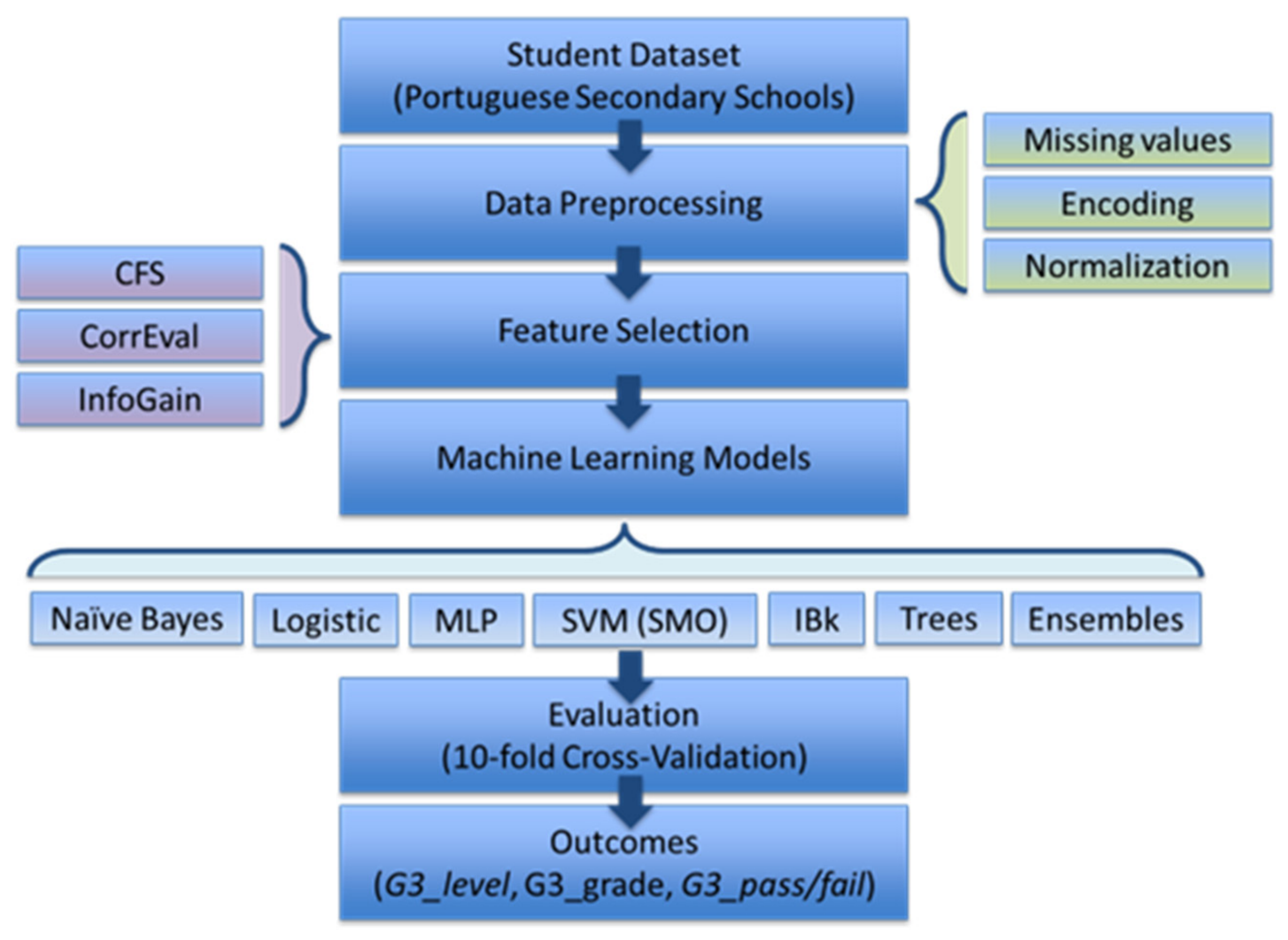
To assess whether the observed differences in classification accuracy among learning algorithms were statistically significant, a Friedman test was conducted on fold-level cross-validation accuracies. The Friedman test is appropriate for comparing multiple classifiers evaluated on repeated measures (cross-validation folds) without assuming normality. If significant differences were observed, average classifier ranks were calculated to compare the algorithms. The proposed workflow diagram of this research is summarized in Figure 1.

2.5. Fairness-Aware Evaluation Considerations

In addition to model performance, fairness constitutes an important consideration when applying ML models in educational contexts. Several variables included in the dataset, such as gender, parental education, and family background, may reflect underlying socio-economic factors rather than purely individual ability.

Although the present study focuses on predictive accuracy and comparative evaluation across models and feature selection methods, fairness-aware evaluation was considered an important methodological dimension. In particular, future analyses could examine model performance across demographic subgroups (e.g., gender or parental education levels) to identify potential disparities in predictive outcomes.

Such subgroup analysis would enable the detection of systematic biases and support the development of more equitable predictive models. While a comprehensive fairness evaluation was not within the scope of this study, its consideration remains essential, especially in the context of deploying predictive models for educational decision-making.

3. Results

3.1. Results of Feature Selection

To gain an initial understanding of the relationships between input variables and the target outcomes, a correlation analysis was first conducted. This step provides insight into the strength and direction of association between individual features and the dependent variables (G3_level, G3_grade, and G3_pass/fail), offering a basis for subsequent feature selection. By identifying variables with stronger associations, this preliminary analysis supports the selection of the most informative predictors and helps reduce dimensionality before applying ML models.

Table 3. Correlation coefficients between input features and outcome variables.

Feature	G3_level	G3_grade	G3_pass/fail
G1	0.81	0.78	0.84
G2	0.77	0.75	0.80
failures	−0.65	−0.62	−0.68
absences	−0.39	−0.36	−0.42
medu	0.35	0.33	0.37
fedu	0.31	0.29	0.34
goout	−0.28	−0.25	−0.23
studytime	0.26	0.24	0.28
schoolsup	0.22	0.20	0.25

presents the correlation coefficients between the selected input features with the strongest associations and the outcome variables.

As shown in Table 3, prior academic indicators, particularly G1, G2, and failures, exhibit the strongest correlations with all outcome variables. In contrast, demographic and behavioral attributes exhibit weaker associations, suggesting a more limited direct influence on academic performance. These findings further justify the application of feature selection techniques to identify the most informative predictors.

The application of the CFS method yielded compact and interpretable feature subsets that are largely consistent with theoretical expectations in educational research, supporting its suitability for comparative analysis across multiple predictive tasks. For the ordinal performance levels (G3_level), the method selected mother’s education (medu), the number of prior course failures (failures), and the second-period grade (G2). For the final grade categorization (G3_grade), the selected subset comprised the home address type (address), the number of prior course failures (failures), the first- and second-period grades (G2, G1), the attendance in preschool (nursery), and relationship status (romantic). Finally, for the binary outcome (G3_pass/fail), the retained features were the student’s sex (sex), the home address type (address), the number of prior course failures (failures), the number of school absences (absences), and the first- and second-period grades (G1, G2).

These results demonstrate the ability of the CFS method to identify both academic and socio-demographic variables that are strongly associated with student achievement. In particular, the consistent selection of failures G1 and G2 across multiple outcomes underscores the dominant predictive role of prior academic performance, a finding consistent with established evidence in educational analytics. At the same time, the inclusion of contextual attributes such as address and nursery for the four-level grade outcome suggests that environmental and early-life factors may exert additional influence on student performance. Overall, CFS proved effective in reducing the feature space to manageable, interpretable subsets, emphasizing the most relevant predictors while mitigating redundancy, an important advantage when working with educational datasets containing many potentially overlapping attributes.

The CorrEval method produced slightly broader feature sets by ranking individual variables according to their pairwise linear association with the target outcome. For G3_level, the selected attributes were the student’s age (age), the number of prior course failures (failures), the peer social engagement (goout), and the first- and second-period grades (G1, G2). For G3_grade, the method identified mother’s education (medu), the number of prior course failures (failures), the student’s age (age), the peer social engagement (goout), and the first- and second-period grades (G1, G2). Finally, for G3_pass/fail, the retained features included mother’s education (medu), the number of prior course failures (failures), the extra educational support (schoolsup), and the first- and second-period grades (G1, G2).

These results further highlight the central importance of academic indicators, as G1, G2 and failures were consistently selected across all outcome definitions. In addition, socio-demographic and behavioral variables emerged as relevant predictors. For example, medu was selected for both the four-level and binary outcomes, highlighting the role of parental education in shaping academic success. Similarly, goout reflecting students’ social activity pattern was associated with both ordinal and four-level performance measures, suggesting that lifestyle factors may have measurable links to achievement. The inclusion of schoolsup for the binary outcome further points to the potential impact of supplementary academic support on course completion. Nevertheless, because this method relies solely on pairwise correlations, it does not explicitly address redundancy among highly correlated predictors. Consequently, closely related variables such as G1 and G2 were frequently selected together. Moreover, nonlinear associations are only captured to the extent that they manifest as monotonic relationships.

When applied to the same prediction tasks, the InfoGain method identified a broader set of informative features. For G3_level, the most informative attributes were the first- and second-period grades (G1, G2), the number of prior course failures (failures), mother’s occupation (mjob), mother’s education (medu), aspiration for higher education (higher), father’s occupation (fjob), and the extra educational support (schoolsup). For G3_grade, InfoGain selected the first- and second-period grades (G1, G2), the number of prior course failures (failures), mother’s occupation (mjob), father’s occupation (fjob), and the extra educational support (schoolsup). For G3_pass/fail, the identified features were the first- and second-period grades (G1, G2), the number of prior course failures (failures), mother’s occupation (mjob), aspiration for higher education (higher), the number of school absences (absences), father’s occupation (fjob), and the extra educational support (schoolsup).

Across all three outcomes, InfoGain consistently emphasized prior academic performance and failure history, confirming their central predictive role. In addition, the method highlighted several socio-economic and aspirational variables, including parental occupation, educational aspirations, and access to supplementary support. This pattern illustrates the capacity of this approach to capture broader contextual influences on academic outcomes by quantifying uncertainty reduction, rather than relying solely on linear associations. However, because it evaluates features independently, it does not account for redundancy or inter-feature interactions. As a result, highly correlated predictors were consistently selected together, leading to slightly larger feature sets compared to CFS.

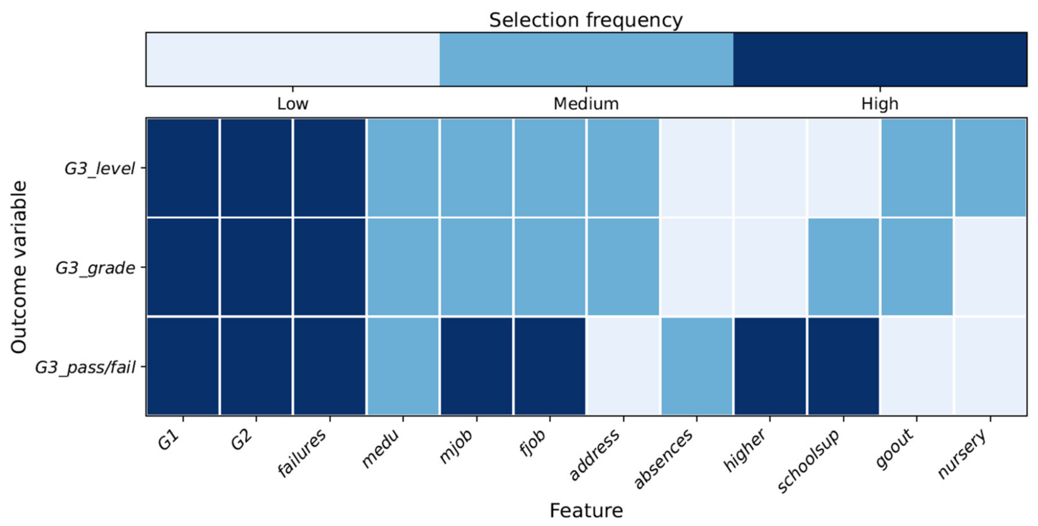
Figure 2 presents a heatmap illustrating the selection frequency (low, medium, high) of each feature across the three outcome definitions (G3_level, G3_grade, G3_pass/fail) and the applied filter-based techniques (CFS, CorrEval, InfoGain). The results indicate that the three procedures provide complementary perspectives. Academic indicators (G1, G2, and failures) were consistently identified as key predictors across all methods and outcomes, underscoring their dominant role in modeling student achievement. In contrast, InfoGain highlighted additional socio-economic and support-related factors (mjob, fjob, higher, schoolsup) that were less emphasized by correlation-based techniques. Overall, these results demonstrate that combining information-theoretic and correlation-based approaches provides a more comprehensive view of the academic, behavioral, and contextual drivers of student performance.

Beyond reporting which variables/features were selected by each method, it is important to interpret why certain socio-demographic attributes emerge or disappear across outcome granularities. The results indicate that the relevance of contextual variables varies according to how academic achievement is defined. For example, parental education and occupation (e.g., medu, mjob, fjob) are selected more often when predicting detailed grade levels (G3_level, G3_grade), where distinguishing between different performance categories requires considering broader socio-economic influences. In contrast, the binary outcome (G3_pass/fail) is mainly driven by prior academic indicators such as G1, G2, and failures, which directly reflect whether a student meets the minimum passing requirement. This suggests that socio-demographic factors are more relevant for explaining differences across performance levels, while recent academic history plays a stronger role in determining simple course completion. Behavioral variables such as goout or schoolsup also appear selectively, depending on whether the outcome captures detailed performance variation or only overall success. Overall, these patterns indicate that feature selection not only reduces dimensionality, but also helps reveal how different definitions of achievement highlight different aspects of students’ academic and social context.

3.2. Classification Accuracy Under Different Feature Selection Methods

This section examines in detail how each combination of feature-selection strategy and ML algorithm performs across three outcomes defined at different levels of granularity derived from the final grade G3 (G3_level, G3_grade, G3_pass/fail). Accuracy scores are macro-averaged across ten-fold stratified cross-validation and compared under four feature-selection conditions: no filtering, CFS, CorrEval, and InfoGain. The ML algorithms employed in this study, as described in Section 2.4, include Naive Bayes, Logistic Regression, Multilayer Perceptron (MLP), Support Vector Machine trained via SMO, k-Nearest Neighbors (IBk, k = 5), Bagging, J48 decision trees, Random Forest, and Random Tree. Model evaluation was intentionally designed to go beyond overall accuracy by incorporating class-wise precision, recall, F1-score, AUC, confusion matrices, statistical testing, and sensitivity analyses.

Table 4. Classification accuracy (%) for G3_level achieved by each machine learning algorithm across different feature selection methods.

Algorithm	Without Feature Selection	CFS	CorrEval	InfoGain
Naive Bayes	82.45	81.95	83.70	84.46
Logistic Regression	83.70	88.97	88.72	88.22
MLP	79.69	88.97	88.47	84.21
SVM (SMO)	78.44	84.46	85.21	81.45
IBk (k = 5)	47.61	87.96	82.45	71.42
Bagging	89.97	89.97	90.47	87.96
J48	86.21	89.72	89.97	89.22
Random Forest	88.47	88.72	88.22	90.72
Random Tree	70.67	87.71	83.95	82.95

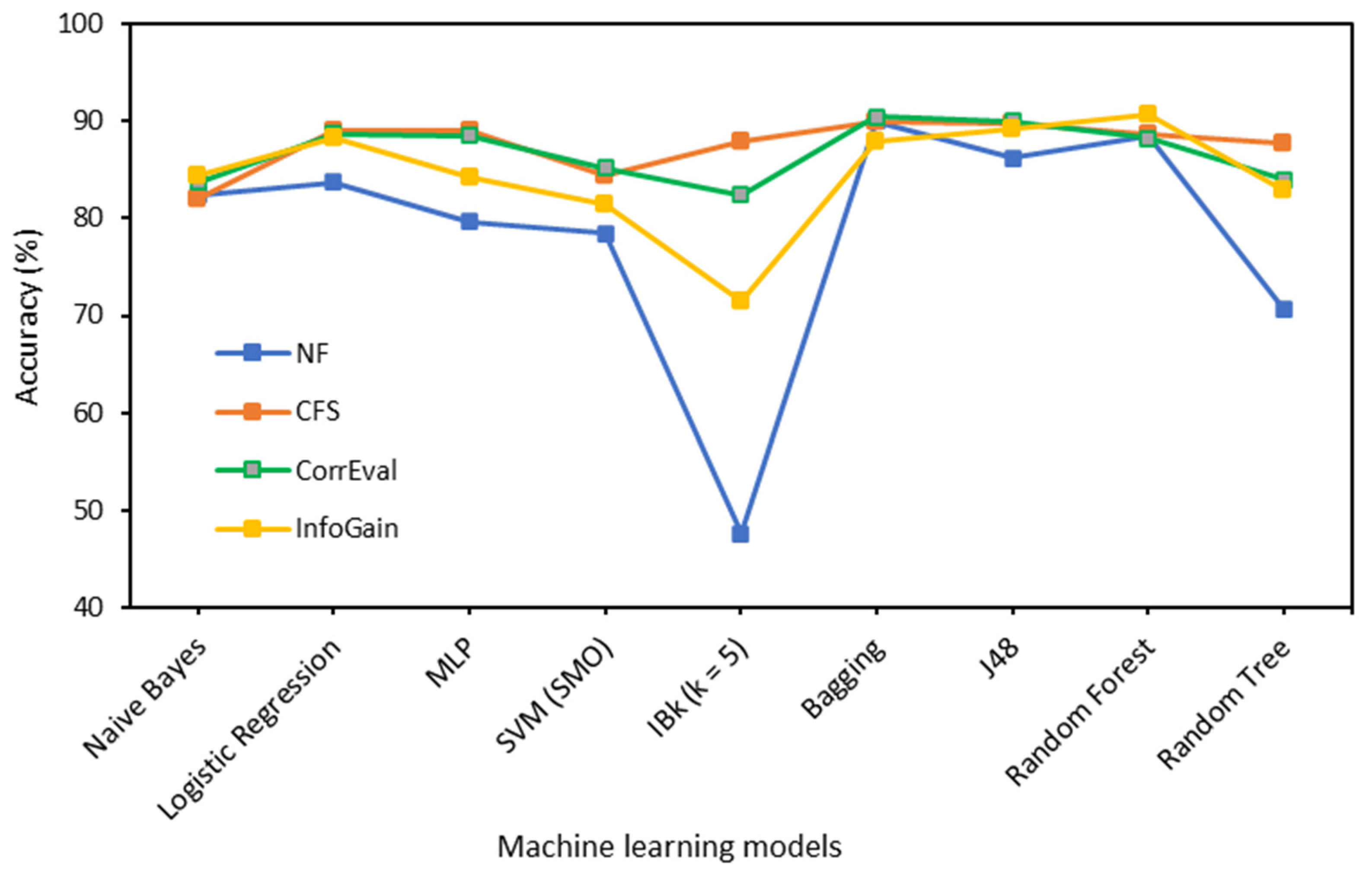
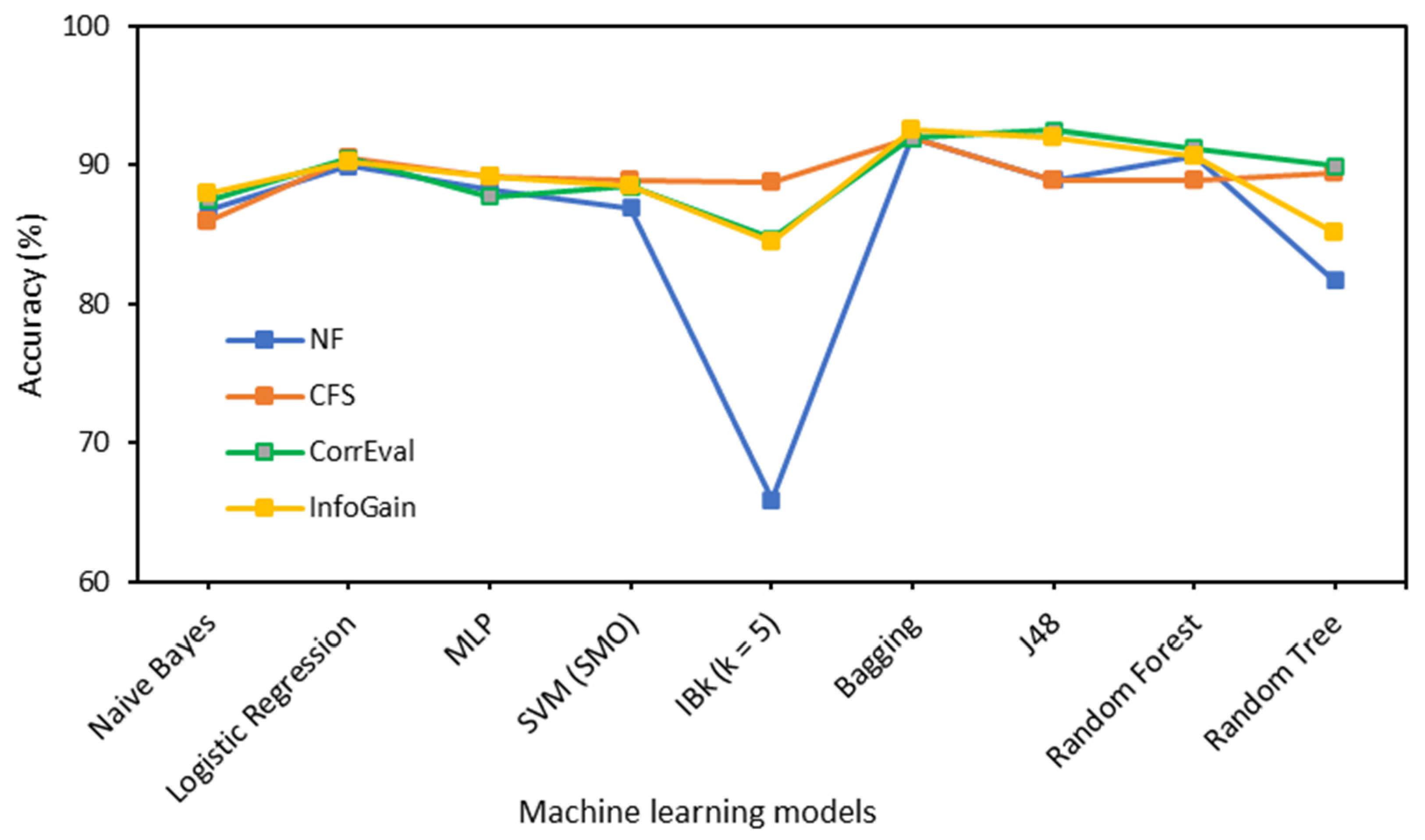
Bold values indicate the highest classification accuracy achieved for each algorithm.

and Figure 3 summarize and compare classification accuracies obtained by the nine ML algorithms under four feature selection settings: no feature selection, CFS, CorrEval, and InfoGain for G3_level. For each classifier, the configuration yielding the highest accuracy is highlighted in Table 4. Although Figure 3 uses line plots for visualization, the categories along the horizontal axis represent nominal variables without inherent ordering. The plots are intended to facilitate comparison of performance across configurations, and no sequential relationship between categories is implied.

Overall, the results demonstrate that feature selection substantially improves predictive performance for most classifiers, particularly for algorithms that are sensitive to feature dimensionality and noise. Performance without feature selection was generally moderate, with most algorithms achieving accuracy levels between 78% and 83%. Notably, IBk performed poorly (47.61%), illustrating the vulnerability of distance-based techniques to irrelevant attributes. Feature selection markedly improved performance. Logistic Regression rose from 83.70% to 88.97% with CFS or CorrEval, while MLP jumped from 79.69% to 88.97% under CFS. These gains suggest that dimensionality reduction sharpens the decision boundaries for both linear and neural models.

Ensemble methods achieved the best results. Bagging with CorrEval reached 90.47%, while Random Forest with InfoGain attained 90.72%, surpassing benchmarks reported in similar educational data mining studies (i.e., Wahdan et al. [53]). Decision tree models remained competitive. J48 achieved 89.97% with CorrEval, confirming that interpretable classifiers can rival black-box ensembles when paired with effective feature filtering. IBk benefited most dramatically, improving by over 40 percentage points when coupled with CFS (from 47.61% to 87.96%), underscoring that irrelevant dimensions disproportionately distort distance computations. Such a finding corroborates the claim by Hall and Holmes [54] that distance metrics suffer from redundant dimensions. The results indicate that combining ensemble models with correlation-based filtering yields highly reliable classifiers, while simpler learners can also achieve strong performance when noise is reduced. The findings further show that both the feature selection technique and the classification algorithm have a significant influence on model performance. Ensemble methods and decision trees, especially Bagging and Random Forest, consistently achieved high accuracy, whereas algorithms such as IBk were more sensitive to feature reduction strategies.

To complement the accuracy-based evaluation, class-wise precision, recall, F1-scores, AUC values and confusion matrix (

Table 5. Class-wise precision, recall, F1-score, AUC and confusion matrix for the best-performing configuration (Random Forest with Information Gain) on the G3_level outcome.

Class	Precision	Recall	F1-Score	AUC	Predicted
					Low	Medium	High	Total
Low	0.92	0.91	0.91	0.95	118	7	2	127
Medium	0.88	0.87	0.87	0.94	6	138	9	153
High	0.90	0.92	0.91	0.96	1	12	102	115
Average/Total	0.90	0.90	0.90	0.95	125	157	113	395

) were computed for the best-performing configuration (Random Forest with InfoGain) on the G3_level prediction task. The model demonstrates strong and balanced performance across all classes, with precision, recall, and F1-scores ranging from 0.87 to 0.92. The macro-averaged F1-score (≈0.90) indicates consistent predictive efficiency across the three levels. The confusion matrix reveals that most misclassifications occur between adjacent categories, particularly for medium-performing students, suggesting that borderline academic profiles are more difficult to distinguish. In contrast, the extreme categories (low and high performance) exhibit higher recall (0.91 and 0.92, respectively), indicating more reliable identification of these groups. The high macro-averaged AUC (0.95) further indicates strong discriminative ability across classes. Overall, these results confirm that Random Forest with InfoGain provides a robust and well-balanced classification of student performance levels.

Table 6. Classification accuracy (%) for G3_grade achieved by each machine learning algorithm across different feature selection methods.

Algorithm	Without Feature Selection	CFS	CorrEval	InfoGain
Naive Bayes	78.94	80.70	80.70	81.20
Logistic Regression	74.18	85.46	84.96	83.95
MLP	72.68	83.70	84.46	81.20
SVM (SMO)	74.43	78.94	77.94	77.19
IBk (k = 5)	40.85	73.93	77.44	67.41
Bagging	86.96	86.96	86.96	85.96
J48	80.95	86.71	86.90	86.71
Random Forest	81.95	84.71	83.95	83.70
Random Tree	63.65	81.95	79.94	77.69

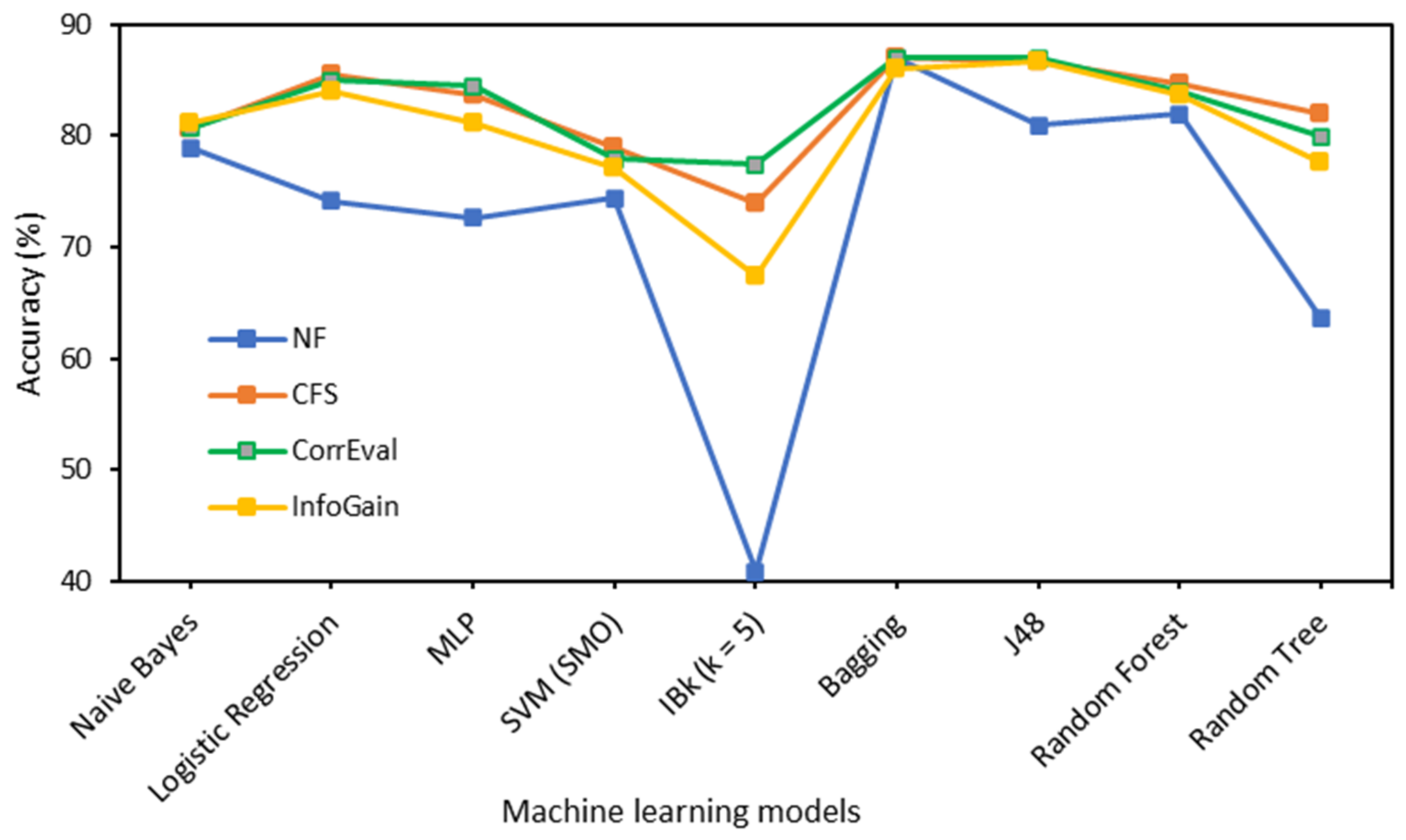
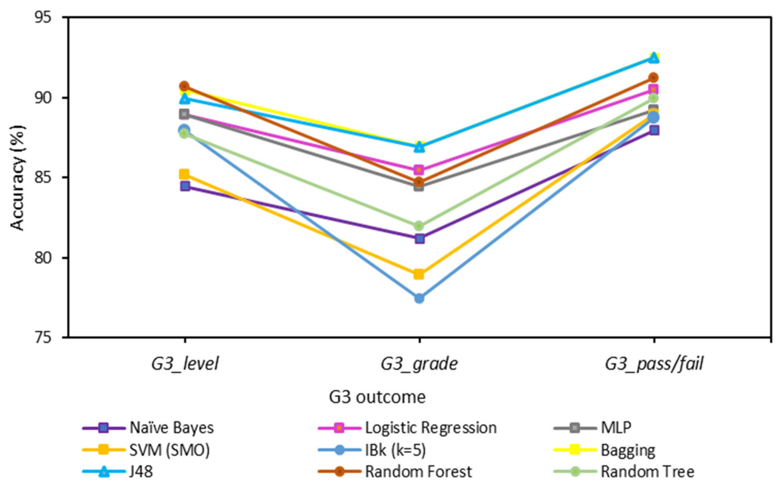
Bold values indicate the highest classification accuracy achieved for each algorithm.

and Figure 4 summarize the classification accuracy obtained by the nine ML algorithms under the four feature selection settings for the four-level categorization of the final grade (G3_grade). The best-performing configuration for each classifier is highlighted in Table 6.

The four-category grade prediction task proved more challenging, as expected, with accuracies dropping relative to the three-class case. Performance without feature selection declined for most models. Logistic Regression (74.18%), MLP (72.68%), and SVM (74.43%) struggled to distinguish between the four grade bands, reflecting the greater complexity of this task. Feature selection mitigated this difficulty. Logistic Regression improved to 85.46% with CFS, while MLP increased to 83.70%. Naive Bayes also showed a modest improvement, rising from 78.94% to 81.20% under InfoGain.

Ensemble and tree-based methods produced the strongest and most consistent performance across feature selection settings. Bagging maintained stable performance at approximately 87% across all configurations, supporting Dietterich’s [55] findings on variance reduction through bootstrap aggregation. Random Forest achieved a maximum accuracy of 84.71% with CFS, while J48 reached 86.90% under CorrEval. Random Tree also showed substantial improvement, increasing from 63.65% without filtering to 81.95% with CFS [56].

Instance-based learning was particularly sensitive to irrelevant features. IBk improved from a near-random accuracy of 40.85% to 77.44% when CorrEval filtering was applied. In contrast, SVM showed only moderate improvement, increasing from 74.43% to 78.94%, suggesting that kernel-based models may require more extensive hyperparameter tuning to fully benefit from feature reduction.

Taken together, the results highlight the importance of feature selection in more granular grade prediction tasks. CFS and CorrEval provided the most consistent improvements across classifiers, while ensemble and tree-based methods maintained strong overall performance. Although the four-level prediction task is inherently more challenging, appropriate feature selection helps mitigate the loss in accuracy.

Table 7. Class-wise precision, recall, F1-score, AUC and confusion matrix for the best-performing configuration (Bagging with Correlation Attribute Evaluation) on the G3_grade outcome.

Class	Precision	Recall	F1-Score	AUC	Predicted
					Fail	Satisfactory	Good	Excellent	Total
Fail	0.89	0.92	0.90	0.96	85	6	1	0	92
Satisfactory	0.85	0.84	0.85	0.94	8	108	9	3	128
Good	0.85	0.82	0.83	0.93	2	10	89	7	108
Excellent	0.86	0.87	0.86	0.95	0	3	6	61	70
Average/Total	0.86	0.86	0.86	0.95	95	127	105	71	395

provides class-wise evaluation metrics and confusion matrix for the best-performing configuration (Bagging with CorrEval) on G3_grade. The classifier shows stable performance across the four grade categories, with precision, recall, and F1-scores ranging from 0.82 to 0.92. The macro-averaged F1-score (≈0.86) indicates balanced performance despite the increased complexity of the four-level prediction task. The confusion matrix shows that most instances are correctly classified, particularly in the Fail and Excellent categories, which achieve the highest recall (0.92 and 0.87, respectively). In contrast, misclassifications mainly occur between adjacent grade levels, especially between Satisfactory and Good, reflecting the difficulty of distinguishing borderline cases. The high macro-averaged AUC (0.95) further indicates strong discriminative ability across classes. Overall, these results suggest that Bagging with CorrEval provides a robust and well-balanced multiclass prediction of final grade outcomes.

Table 8. Classification accuracy (%) for G3_pass/fail achieved by each machine learning algorithm across different feature selection methods.

Algorithm	Without Feature Selection	CFS	CorrEval	InfoGain
Naive Bayes	86.71	85.96	87.46	87.96
Logistic Regression	89.97	90.47	90.47	90.22
MLP	88.22	89.22	87.71	89.22
SVM (SMO)	86.96	88.97	88.47	88.47
IBk (k = 5)	65.91	88.72	84.71	84.46
Bagging	91.97	91.97	91.97	92.48
J48	88.97	88.97	92.48	91.97
Random Forest	90.72	88.97	91.22	90.72
Random Tree	81.70	89.47	89.97	85.21

Bold values indicate the highest classification accuracy achieved for each algorithm.

and Figure 5 present the classification accuracy of the nine ML algorithms across the four feature selection settings for G3_pass/fail. The best-performing configuration for each classifier is highlighted in Table 8.

As expected, binary classification produced the strongest results overall, with high accuracy observed even without feature selection for most ML algorithms. Logistic Regression achieved 89.97% without filtering and improved to 90.47% with both CFS and CorrEval, demonstrating both strong performance and stability. MLP also maintained high accuracy across all configurations (87.71–89.22%), reflecting its robustness to different feature subsets. Random Forest reached 90.72%, further confirming that the pass/fail distinction is relatively easier to model.

Across most classifiers, accuracy was high and generally improved after applying feature selection techniques [2]. Bagging with InfoGain and J48 with CorrEval both achieved 92.48%, the highest values across all tasks, suggesting strong performance of ensemble and tree-based methods for binary outcomes. Random Forest, another ensemble method, reached 91.22% with CorrEval and remained above 88% across all configurations, confirming its effectiveness. Probabilistic and margin-based classifiers also benefited: Naive Bayes peaked at 87.96% with InfoGain, while SVM improved from 86.96% to 88.97% with CFS. IBk showed the largest gain, increasing from 65.91% without feature selection to 88.72% with CFS, highlighting its sensitivity to irrelevant or noisy features [37].

Overall, feature selection improved or preserved performance across most classifiers. Ensemble methods (Bagging and Random Forest) achieved the highest accuracy, followed closely by Logistic Regression and MLP. While binary tasks are inherently simpler, ensemble classifiers provided an additional advantage, reaching accuracies above 92%. These findings also emphasize the importance of feature selection, particularly for algorithms such as IBk, which are more sensitive to high-dimensional data.

Table 9. Class-wise precision, recall, F1-score, AUC and confusion matrix for the best-performing configuration (Bagging with Information Gain) on the G3_pass/fail outcome.

Class	Precision	Recall	F1-Score	AUC	Predicted
					Fail	Pass	Total
Fail	0.85	0.95	0.90	0.96	127	6	133
Pass	0.98	0.92	0.95	0.96	22	240	262
Average/Total	0.91	0.94	0.92	0.96	149	246	395

presents class-wise evaluation metrics and the confusion matrix for the best-performing configuration (Bagging with InfoGain) on the G3_pass/fail prediction task.

The model achieves strong predictive performance, with a macro-averaged F1-score of approximately 0.92 and an AUC of 0.96, indicating excellent discrimination between the two classes. The confusion matrix shows that most instances are correctly classified, with particularly high recall for the Fail class (0.95), correctly identifying 127 out of 133 students. Only a small number of failing students are misclassified as passing, reducing the risk of overlooking at-risk individuals. For the Pass class, the model also performs well, with high precision (0.98) and recall (0.92). Most errors occur when passing students are predicted as failing, slightly increasing false positives while maintaining strong detection of failing cases. Overall, the high F1-scores and AUC values indicate a well-balanced model for distinguishing between passing and failing students.

Figure 6 summarizes the highest classification accuracy achieved by each ML algorithm across the three outcome definitions (G3_level, G3_grade, and G3_pass/fail), considering all feature selection configurations.

The comparison of results across the three outcome variables (G3_level, G3_grade, and G3_pass/fail) reveals several important trends related to algorithm performance, feature selection, and predictive complexity. Ensemble methods such as Bagging and Random Forest consistently achieved the highest accuracy in both binary and multiclass tasks. Bagging performed best in the binary setting and also showed strong results in multiclass scenarios, especially when combined with CorrEval for G3_level and G3_grade. These findings highlight the interaction between outcome granularity, feature selection, and classifier choice in student performance prediction.

Feature selection proved beneficial across all tasks, particularly for algorithms sensitive to high-dimensional data, such as IBk and SVM (SMO). IBk, which performed poorly without feature selection, showed substantial accuracy gains when combined with CFS and CorrEval, highlighting its reliance on a reduced and relevant feature space. Similarly, SVM showed more stable and improved results after feature selection, suggesting that its decision boundaries benefit from noise reduction and more informative attributes.

Logistic Regression and MLP classifiers exhibited robust and stable performance across all representations of G3. Logistic Regression showed notable improvement after feature selection for both G3_level and G3_grade. MLP followed closely, demonstrating consistent adaptability, especially with CFS and CorrEval, although it slightly trailed Logistic Regression in some cases.

Naive Bayes, although not the top-performing model, demonstrated consistent moderate accuracy. It benefited from feature selection, particularly InfoGain and CorrEval, achieving its best results in the G3_pass/fail and G3_level tasks. These findings suggest that, despite its simplicity, Naive Bayes remains a useful baseline for educational data classification when combined with appropriate preprocessing.

In terms of outcome complexity, G3_pass/fail, as a binary task, achieved the highest accuracy across all classifiers, indicating that the simpler decision boundary is easier for models to learn. In contrast, G3_grade, with four distinct categories, posed greater challenges and resulted in lower performance, even for top-performing algorithms. G3_level, with three ordinal classes, showed intermediate performance levels between the binary and four-class settings. Overall, prediction was easiest for the binary pass/fail task (>92%), moderately difficult for the three-level classification (≈90%), and most challenging for the four-grade task (≈87%).

Among the feature selection methods, CorrEval consistently led to the highest or near-highest accuracy, particularly when combined with Bagging and J48. InfoGain also produced strong results, although its impact was less pronounced in some configurations, while remaining particularly effective in binary tasks. CFS often resulted in noticeable improvements, especially for algorithms that do not perform internal feature weighting or selection [13].

To assess whether performance differences among classifiers were statistically significant, a Friedman test was applied to fold-level cross-validation accuracies under the InfoGain setting. The test compares the performance of multiple classifiers across repeated cross-validation folds. For all three target variables (G3_level, G3_grade, and G3_pass/fail), the test indicated statistically significant differences (χ² = 38.26, p < 0.001; χ² = 29.86, p < 0.001; and χ² = 25.46, p < 0.01, respectively), indicating that at least one classifier differed significantly in performance.

Table 10. Average classifier ranks based on the Friedman test under Information Gain feature selection for the three outcomes.

Model	G3_level	G3_grade	G3_pass/fail
Logistic Regression	3.15	2.95	3.20
Random Forest	3.30	3.70	3.00
Bagging	3.80	5.05	4.55
MLP	4.20	4.90	4.10
IBk (k = 5)	4.65	3.60	4.90
SVM (SMO)	4.95	4.20	5.40
J48	5.75	5.95	5.70
Random Tree	6.20	6.75	6.70
Naive Bayes	9.00	7.90	7.45

presents the average classifier ranks derived from this analysis. Logistic Regression and Random Forest achieved the best overall ranks across the three targets, indicating stable performance. Ensemble techniques generally achieved higher ranks than single-tree models, while Naive Bayes consistently ranked lowest.

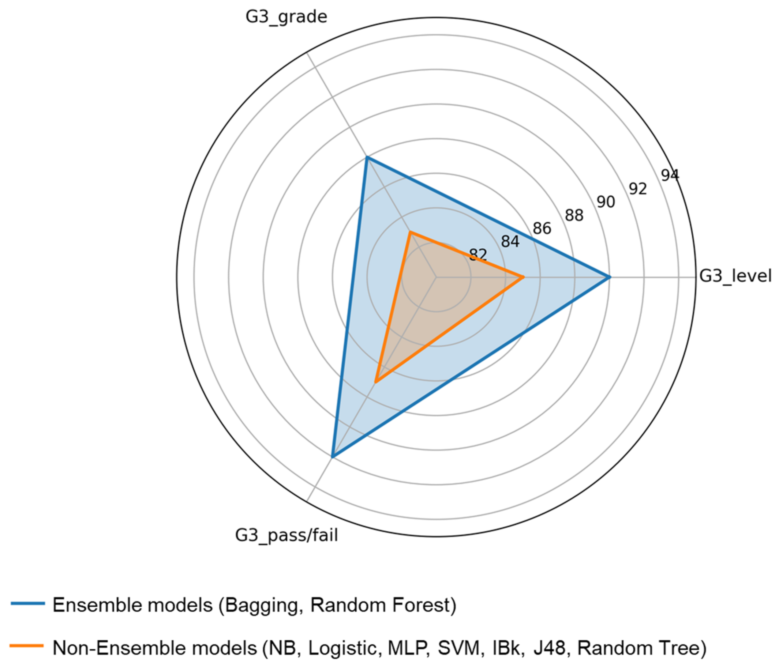
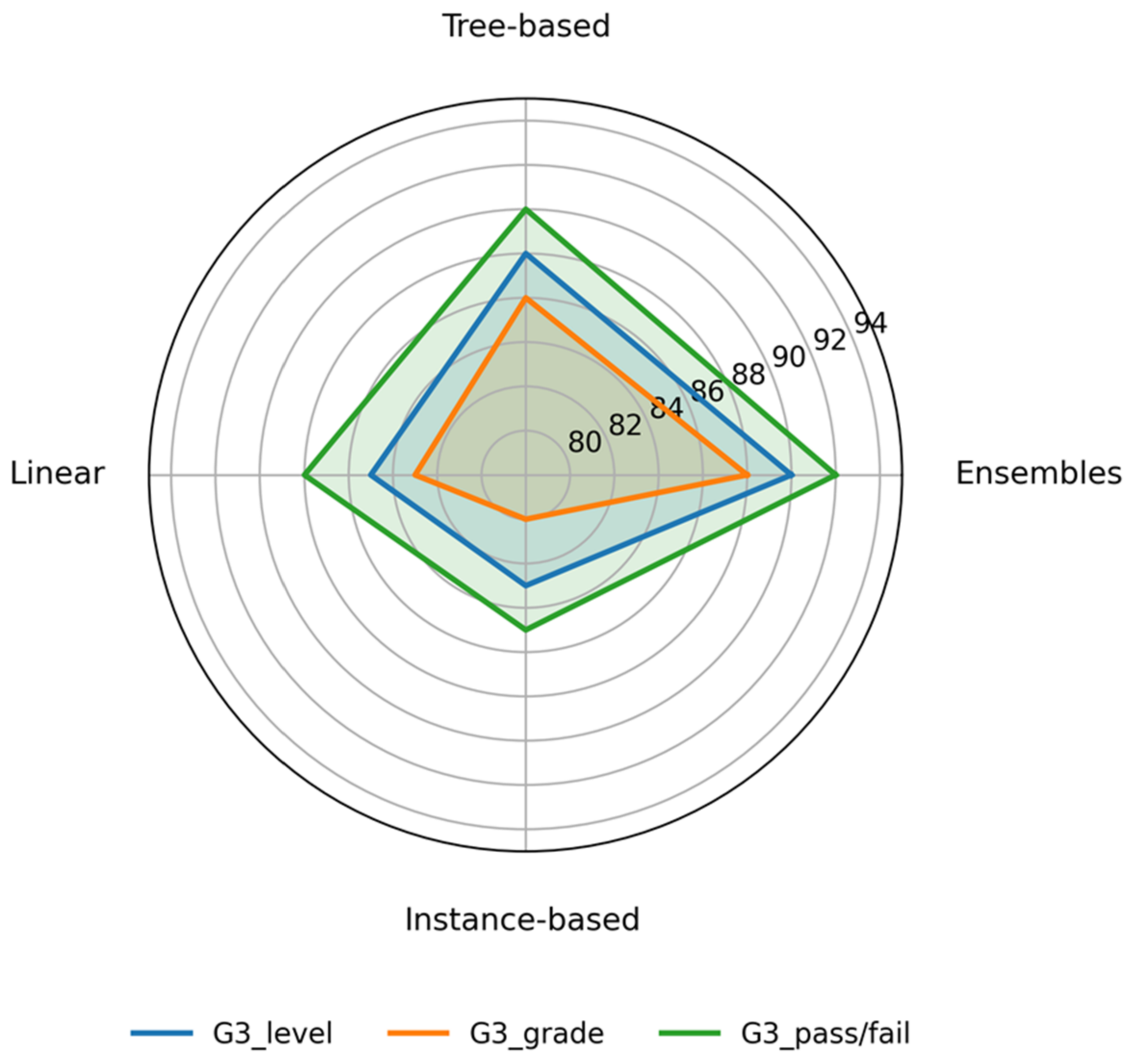
In addition to individual classifier comparisons, the results are summarized using two radar charts that provide an aggregated view of model performance across outcome granularities. Figure 7 contrasts ensemble (Bagging, Random Forest) and non-ensemble models (all other models), highlighting differences in average classification accuracy across the three outcomes. Figure 8 extends this analysis by grouping classifiers into four model families: ensemble (Bagging, Random Forest), tree-based (J48, Random Tree), linear (Logistic Regression), and instance-based (IBk), offering a higher-level comparison of learning paradigms. Together, these visualizations complement the classifier-level results by emphasizing overall performance trends and robustness patterns across outcome definitions.

As shown in the figures, ensemble models generally achieve the highest average accuracy across all outcome definitions (G3_level, G3_grade, and G3_pass/fail), demonstrating strong robustness to changes in outcome granularity. In contrast, linear and instance-based models show greater variability, particularly for more complex outcome formulations, while tree-based approaches exhibit more stable intermediate performance.

Key features remain stable across methods. Prior academic performance (G1, G2) and failure history (failures) appear in all top-performing models, reaffirming their central role in predicting achievement and aligning with the academic-momentum theory of Sticca et al. [57]. The consistent presence of socio-supportive features (schoolsup, higher, address, nursery) further highlights that environmental and aspirational factors may also influence performance trajectories. From a practical perspective, ensemble models such as Bagging and Random Forest can serve as high-accuracy components of early warning systems, while interpretable models like J48 provide transparent decision rules for policy applications.

Overall, the findings indicate that ensemble classifiers provide a robust modeling approach for educational datasets, particularly when combined with attribute evaluation techniques such as CorrEval and InfoGain. While binary outcomes are easier to predict, with accuracies exceeding 90%, multiclass outcomes, such as G3_grade and G3_level, require more careful feature selection and model design to achieve comparable performance. The consistent performance of Bagging and J48 across all grade representations further supports their suitability for educational data mining applications.

Beyond predictive performance, the use of socio-demographic attributes in educational models raises important considerations regarding fairness and potential bias. Variables such as gender, parental education, and family background can enhance predictive robustness, but they also reflect structural socio-economic conditions that are largely beyond students’ control. The observed distributional patterns indicate that lower academic outcomes are more prevalent among students from less advantaged backgrounds, reflecting well-documented educational inequalities rather than differences in individual ability. If used without careful interpretation, such models may inadvertently reproduce or amplify these inequalities. In this study, socio-demographic attributes were included solely for comparative purposes, to examine their predictive contribution across outcome granularities, and not for automated decision-making. It should also be noted that the present study does not include a formal fairness evaluation across demographic groups. The results also show that prior academic performance remains the dominant predictor, particularly in binary settings, while socio-demographic variables play a secondary and context-dependent role. Future applications should include fairness-aware evaluation and bias mitigation strategies to ensure equitable outcomes. When used responsibly, predictive models can support early identification of at-risk students, complementing, rather than replacing, human judgment in educational decision-making.

3.3. Sensitivity Analysis of Imputation Methods

To evaluate the robustness of the proposed models with respect to the imputation strategy, a sensitivity analysis was conducted comparing mean/mode imputation with k-Nearest Neighbors (kNN, k = 5). The analysis focused on the best-performing model configurations across the three outcomes.

Table 11. Classification accuracy (%) under different imputation methods (mean/mode vs. kNN, k = 5) for selected model configurations.

Model	Outcome	Mean/Mode	kNN (k = 5)	Difference
Random Forest + InfoGain	G3_level	90.72	91.13	+0.41
Random Forest + InfoGain	G3_grade	84.71	85.18	+0.47
Random Forest + InfoGain	G3_pass/fail	91.22	91.78	+0.56
Bagging + CorrEval	G3_level	90.47	90.89	+0.42
Bagging + CorrEval	G3_grade	86.96	87.48	+0.52
Bagging + InfoGain	G3_pass/fail	92.48	92.91	+0.43
Logistic Regression + CFS	G3_level	88.97	89.39	+0.42
Logistic Regression + CFS	G3_grade	85.46	85.98	+0.52

summarizes the results of the sensitivity analysis.

As shown in Table 11, the differences in classification accuracy between the two imputation methods are minimal, generally remaining below 0.6% across all evaluated cases. These results indicate that the impact of the imputation strategy on model performance is minimal. Furthermore, the relative ranking of classifiers and feature selection techniques remains consistent across imputation approaches. High-performing models, such as Random Forest with InfoGain and Bagging configurations, retain their superior predictive performance regardless of the imputation method. Overall, these findings confirm that the results of this study are robust and not driven by the choice of imputation technique, thereby supporting the validity and robustness of the comparative evaluation.

3.4. Early Prediction Experiments Excluding Prior Grades

To examine the early intervention potential of the proposed framework, additional experiments were conducted after excluding the prior grade variables G1 and G2 from the feature set. As these variables represent intermediate assessments close to the final outcome (G3), their inclusion may reduce the practical applicability of predictive models for early identification of at-risk students. Removing these variables enables the evaluation of models based solely on demographic, behavioral, and contextual attributes available at earlier stages of the academic process. To ensure consistency, the same preprocessing procedures, feature selection methods (CFS, CorrEval, and InfoGain), and ML algorithms were applied. Model evaluation was again performed using stratified ten-fold cross-validation.

Considering feature selection for the G3_level prediction task, all methods consistently identified failures as a highly informative attribute, underscoring the strong influence of prior academic difficulties on future performance. The CFS method selected a compact subset consisting of failures, medu, and higher, suggesting that parental education and students’ intention to pursue higher education are important indicators of academic achievement. CorrEval identified failures, age and goout, indicating that maturity and social activity patterns may also contribute to variation in performance levels. InfoGain produced a slightly larger feature set, including failures, mjob, medu, higher, fjob, and schoolsup, highlighting the potential influence of family background and additional academic support in explaining variations in student outcomes.

For the G3_grade outcome, the selected features varied more substantially across the methods, reflecting the increased complexity of predicting four distinct grade categories. CFS emphasized contextual and social factors such as address, nursery, and romantic, along with failures, suggesting that environmental and social conditions may influence finer distinctions in academic performance. In contrast, CorrEval highlighted demographic and behavioral attributes including medu, age, goout, and failures, while InfoGain prioritized family and support-related variables such as mjob, fjob, schoolsup, higher, and failures.

For the G3_pass/fail outcome, the CFS method retained failures, famsize, reason, schoolsup, internet, and goout, indicating the relevance of family background, school motivation, academic support, and student engagement. CorrEval selected failures, age, goout, higher, and paid, emphasizing behavioral patterns and educational aspirations. InfoGain produced a more compact subset consisting of failures, goout, and age, suggesting that these variables provide the strongest predictive contribution when intermediate grades are unavailable. Notably, failures and goout were consistently identified across methods, highlighting the importance of accumulated academic difficulty and behavioral engagement for early-stage prediction.

Table 12. Classification accuracy (%) for G3_level achieved by each machine learning algorithm across different feature selection methods excluding prior grades (G1 and G2) from the feature set.

Algorithm	Without Feature Selection	CFS	CorrEval	InfoGain
Naive Bayes	49.11	51.14	50.38	51.39
Logistic Regression	47.59	50.63	52.15	52.15
MLP	44.81	49.37	48.10	50.13
SVM (SMO)	46.84	50.13	51.39	51.65
IBk (k = 5)	42.53	48.61	47.85	49.87
Bagging	50.63	51.65	51.90	52.41
J48	45.82	49.87	50.89	51.39
Random Forest	48.61	50.13	50.63	51.14
Random Tree	41.77	46.84	47.34	49.11

Bold values indicate the highest classification accuracy achieved for each algorithm.

summarizes the classification accuracy obtained by the nine ML algorithms across different feature selection methods (without feature selection, CFS, CorrEval, and InfoGain) for G3_level after excluding prior grades (G1 and G2) from the feature set. The best-performing configuration for each classifier appears highlighted.

The overall predictive performance decreases substantially compared to experiments that include prior academic indicators. Accuracy across all algorithms and configurations ranges between approximately 41% and 52%, highlighting the strong influence of previous grades on student achievement prediction. Despite this reduction, feature selection consistently improves model performance compared to using the full feature set, with the highest accuracies typically achieved under InfoGain. Ensemble methods demonstrate relatively stable performance under this setting, with Bagging reaching the highest accuracy of 52.41%. In contrast, instance-based learning (IBk) and Random Tree demonstrate lower predictive performance, although they also benefit from feature filtering.

Table 13. Class-wise precision, recall, F1-score, AUC and confusion matrix for the best-performing configuration (Bagging with Information Gain) on the G3_level outcome without prior grades.

Class	Precision	Recall	F1-Score	AUC	Predicted
					Low	Medium	High	Total
Low	0.64	0.67	0.65	0.74	55	18	9	82
Medium	0.66	0.66	0.66	0.75	21	88	24	133
High	0.81	0.79	0.80	0.82	10	27	143	180
Average/Total	0.70	0.71	0.70	0.77	86	133	176	395

presents class-wise evaluation metrics and the confusion matrix for the best-performing configuration (Bagging with InfoGain) on the G3_level prediction task without G1 and G2. Overall performance decreases compared to models that include prior academic information, with a macro-averaged F1-score of approximately 0.70 and an AUC of 0.77, indicating moderate discriminative capability. The model performs best for the High-performance category, achieving the highest precision, recall, and F1-score. In contrast, the Low and Medium categories show lower and more balanced scores, reflecting greater difficulty in distinguishing these levels without prior grade information. The confusion matrix indicates that most errors occur between adjacent categories, particularly between Low and Medium and between Medium and High, suggesting increased ambiguity in predicting borderline cases.

Table 14. Classification accuracy (%) for G3_grade achieved by each machine learning algorithm across different feature selection methods excluding prior grades (G1 and G2) from the feature set.

Algorithm	Without Feature Selection	CFS	CorrEval	InfoGain
Naive Bayes	46.33	47.85	47.34	48.10
Logistic Regression	44.56	47.34	48.10	48.61
MLP	42.78	45.82	46.58	47.59
SVM (SMO)	43.80	46.84	47.59	47.09
IBk (k = 5)	40.76	45.06	45.57	47.85
Bagging	46.58	47.34	48.10	48.61
J48	43.29	46.33	47.09	47.59
Random Forest	45.06	46.33	46.84	47.34
Random Tree	39.24	42.78	44.30	45.82

Bold values indicate the highest classification accuracy achieved for each algorithm.

presents the classification accuracy of the evaluated ML algorithms for the G3_grade task after excluding prior grades (G1 and G2), with the best-performing feature selection configuration highlighted. Overall, performance declines substantially compared to models that include prior academic information, with accuracy ranging from approximately 39% to 49% across classifiers. Despite this reduction, feature selection consistently improves results, with InfoGain and CorrEval generally yielding the highest accuracy. The best performance is achieved by Logistic Regression and Bagging with InfoGain, both reaching 48.61%. In contrast, IBk and Random Tree remain among the weaker performers. These findings further confirm the dominant predictive role of prior grades.

Table 15. Class-wise precision, recall, F1-score, AUC and confusion matrix for the best-performing configuration (Bagging with Information Gain) on the G3_grade outcome without prior grades.

Class	Precision	Recall	F1-Score	AUC	Predicted
					Fail	Satisfactory	Good	Excellent	Total
Fail	0.55	0.62	0.58	0.72	46	18	8	2	74
Satisfactory	0.51	0.52	0.51	0.71	22	59	26	7	114
Good	0.55	0.54	0.54	0.73	12	30	68	16	126
Excellent	0.65	0.58	0.61	0.76	4	9	21	47	81
Average/Total	0.56	0.56	0.56	0.73	84	116	123	72	395

presents class-wise evaluation metrics and the confusion matrix for the best-performing configuration (Bagging with InfoGain) on the G3_grade task without G1 and G2. Overall performance decreases compared to models that include prior academic indicators, with a macro-averaged F1-score of 0.56 and an AUC of 0.73, indicating moderate predictive ability. The Excellent category shows the strongest performance, suggesting that top-performing students can still be identified relatively reliably. In contrast, the Fail, Satisfactory, and Good categories exhibit lower and similar F1-scores, reflecting greater difficulty in distinguishing intermediate levels. The confusion matrix indicates that most errors occur between adjacent categories, particularly between Satisfactory and Good, and between Good and Excellent, highlighting increased ambiguity in predicting more precise grade distinctions without prior grade information.

Table 16. Classification accuracy (%) for G3_pass/fail achieved by each machine learning algorithm across different feature selection methods excluding prior grades (G1 and G2) from the feature set.

Algorithm	Without Feature Selection	CFS	CorrEval	InfoGain
Naive Bayes	70.17	70.92	70.42	70.92
Logistic Regression	68.42	70.67	71.17	72.15
MLP	61.91	67.41	66.41	69.67
SVM (SMO)	67.41	69.92	71.67	71.42
IBk (k = 5)	61.91	67.91	67.16	72.18
Bagging	69.17	67.41	70.42	72.35
J48	64.91	67.91	70.17	71.42
Random Forest	68.42	66.91	68.17	69.92
Random Tree	59.89	62.65	64.16	70.17

Bold values indicate the highest classification accuracy achieved for each algorithm.

summarizes the classification accuracy of the nine ML algorithms for the G3_pass/fail outcome without prior grades. Despite the absence of these predictors, the models retain meaningful performance, particularly when feature selection is applied. Several classifiers achieve accuracy levels around or above 70%, especially with InfoGain and CorrEval. Logistic Regression, SVM, IBk, and tree-based models demonstrate competitive results, while ensemble methods remain relatively stable.

Table 17. Class-wise precision, recall, F1-score, AUC and confusion matrix for the best-performing configuration (Bagging with Information Gain) on the G3_pass/fail outcome without prior grades.

Class	Precision	Recall	F1-Score	AUC	Predicted
					Fail	Pass	Total
Fail	0.57	0.71	0.63	0.78	94	39	133
Pass	0.83	0.73	0.78	0.78	70	192	262
Average/Total	0.70	0.72	0.71	0.78	164	231	395

presents class-wise evaluation metrics and the confusion matrix for the best-performing configuration (Bagging with InfoGain) on the G3_pass/fail task without G1 and G2. Overall performance decreases compared to models that incorporate prior academic information, with a macro-averaged F1-score of 0.71 and an AUC of 0.78, indicating moderate discriminative ability. The model performs better for the Pass class, correctly identifying most passing students. In contrast, the Fail class shows lower precision but relatively high recall, indicating that most failing students are detected, although some passing students are misclassified. The confusion matrix indicates that most errors occur when passing students are predicted as failing, reflecting increased uncertainty in predicting student outcomes without prior grade information.

The results across the three grade granularities indicate that, in the absence of prior grades (G1 and G2), model performance declines substantially. Nevertheless, for binary risk identification, demographic, behavioral, and school-related variables still provide meaningful predictive signals. This finding suggests that the proposed framework retains practical relevance for early intervention, particularly for identifying students at risk of failing before intermediate grades become available.

Although prior academic indicators such as G1, G2, and previous failures significantly improve predictive accuracy, their proximity to the final outcome limits their usefulness for early intervention. The aim of this study was not to develop models based solely on pre-course or demographic variables, but to examine how feature selection and ML methods behave across different grade granularities. The experiments excluding prior grades therefore provide an exploratory assessment of model behavior without near-outcome academic indicators. The results highlight the distinction between models optimized for predictive accuracy and those designed for early warning systems, which must rely on information available at earlier stages of the academic process.

4. Conclusions

This study investigates the combined impact of feature selection and machine learning classifiers on the prediction of secondary school achievement across three grade granularities, using a well-established benchmark dataset from Portuguese secondary education. By evaluating nine classifiers under three widely used filter-based feature selection strategies, it offers a comprehensive comparison of how predictive efficiency, robustness, and interpretability vary with outcome definition and preprocessing choices.

The results show that ensemble classifiers, particularly Random Forest and Bagging, consistently achieved the highest accuracy across all outcome representations, demonstrating their robustness to noise, redundancy, and complex feature interactions. Information Gain emerged as a consistently effective filtering technique, especially for multiclass tasks with more complex decision boundaries. In contrast, Correlation-based Feature Subset Selection (CFS) proved particularly beneficial for algorithms sensitive to multicollinearity and high dimensionality, such as k-Nearest Neighbors and linear models, improving performance through redundancy-aware feature reduction.

Across all configurations, prior academic performance indicators, notably first- and second-period grades and failure history, were consistently identified as the most influential predictors, reaffirming the central role of academic momentum in shaping educational outcomes. In addition, socio-contextual and support-related variables, including parental education and occupation, early schooling experiences, and access to supplementary educational support, contributed meaningfully to predictive accuracy, particularly when information-theoretic feature selection was applied.

The experiments excluding prior grades (G1 and G2) highlight the critical role of previous academic performance in predicting student outcomes. Without these variables, model performance decreases substantially across all outcome representations, confirming that prior achievement is the most informative predictor of future success. Nevertheless, demographic, behavioral, and family-related attributes still provide some predictive value, enabling models such as Bagging with Information Gain to achieve moderate performance. These findings indicate that, although prior grades remain dominant, alternative socio-educational features can still support the early identification of academically at-risk students.

From an intervention perspective, the findings suggest that different types of predictors may be useful at different stages of the academic process. Relatively static variables, such as parental education, parental occupation, family background, and previous course failures, are typically available before the school year begins and may help schools identify students who may be academically vulnerable even before academic difficulties become visible. These variables can support early screening efforts and allow institutions to provide preventive support at the beginning of the academic year. In contrast, dynamic behavioral indicators, such as absences and behavioral indicators, become available as the semester progresses and can help schools update risk assessments based on changes in student engagement. For example, there may be a student who begins the semester with no obvious academic concerns may subsequently exhibit increasing absenteeism, reduced study time, or declining participation in school-related activities. These changes may signal emerging academic risk and allow educators to intervene before poor final outcomes become evident.

It is also important to consider what types of students may be identified by predictive models but may not be easily recognized through teacher observation alone. Poor performance in G1 and G2 is usually visible to teachers and may not require algorithmic support. However, students with average or acceptable early grades may still be at risk due to combinations of factors that are less apparent in everyday classroom settings. For example, students experiencing gradual increases in absenteeism, limited family support, socio-economic disadvantages, low educational aspirations, or recurring behavioral difficulties may not immediately be identified as at risk if their short-term academic performance remains stable. Similarly, some students may not exhibit a single clear warning sign but may instead face several moderate risk factors that, when combined, increase the likelihood of poor academic outcomes. For example, a student may maintain average grades while also showing slightly increased absenteeism, limited parental educational support, lower motivation for higher education, and reduced study time. Individually, these factors may not appear alarming to teachers, but when considered collectively, may indicate elevated academic risk that is more difficult to detect through traditional classroom observation alone. In this sense, predictive models should therefore be regarded as complementary decision-support tools that can help schools detect less visible risk patterns and support earlier and more targeted interventions, rather than simply confirming problems that teachers already recognize.

From a practical perspective, the findings support a dual-layer modeling strategy that balances accuracy and interpretability. High-performing ensemble models can be used for early-warning and triage, while interpretable classifiers such as pruned decision trees provide transparent decision rules for pedagogical decision-making and policy-oriented applications. Moreover, the multi-granularity evaluation shows that while binary pass/fail outcomes are easier to predict, careful feature selection enables robust performance even in more challenging multiclass scenarios.

Although the dataset used in this study is a widely recognized benchmark in educational data mining, it reflects a specific context within Portuguese secondary education. While the proposed framework is methodologically transferable, its predictive performance and the relative importance of predictors may vary across educational systems due to differences in grading schemes, institutional structures, and socio-economic conditions. The empirical findings should therefore be interpreted within this specific national educational context. For example, the 0–20 grading scale used in Portugal and the classification of parental occupation may not directly correspond to systems based on letter grades or alternative socio-economic categorizations. Future research may also explore institutional, regional, and cross-national variability in predictor importance. Furthermore, model evaluation relies on cross-validation within a single dataset. Although this provides robust internal estimates, external validation using independent datasets, cross-school comparisons, or temporal validation would offer stronger evidence of generalizability. Future work should validate the proposed framework using independent datasets from different educational systems and longitudinal cohorts to further assess external validity and temporal robustness. Despite these limitations, the observed comparative patterns, particularly the consistent importance of prior academic performance and the effectiveness of feature selection methods, are likely to generalize to similar educational data mining contexts. These findings provide useful methodological insights for the development of predictive models in other educational contexts.

External validation using independent datasets, cross-school comparisons, and temporal splits represents an important direction for future research to assess the robustness and transferability of the proposed framework. In particular, evaluating temporal generalizability across academic years and student cohorts would provide stronger evidence of model stability over time. Extending the analysis to additional educational contexts and incorporating longitudinal or behavioral data may further improve understanding of the dynamics underlying student achievement. Overall, this study provides empirical support for the effective integration of feature selection and ensemble learning as a robust and methodologically reliable framework for predictive analytics in secondary education.

References

1. Baker, R.S.; Siemens, G. Educational data mining and learning analytics. In The Cambridge Handbook of the Learning Sciences, 2nd ed.; Part II. Methodologies; Sawyer, K.A., Ed.; Cambridge University Press: Cambridge, UK, 2014; pp. 253–272. [Google Scholar]
2. Romero, C.; Ventura, S. Educational data mining and learning analytics: An updated survey. WIREs Data Min. Knowl. 2020, 10, e1355. [Google Scholar] [CrossRef] [Scilit]
3. Peña-Ayala, A. Educational data mining: A survey and a data mining-based analysis of recent works. Expert Syst. Appl. 2014, 41, 1432–1462. [Google Scholar] [CrossRef] [Scilit]
4. López-Meneses, E.; Mellado-Moreno, P.C.; Gallardo Herrerías, C.; Pelícano-Piris, N. Educational Data Mining and Predictive Modeling in the Age of Artificial Intelligence: An In-Depth Analysis of Research Dynamics. Computers 2025, 14, 68. [Google Scholar] [CrossRef] [Scilit]
5. Kizilcec, R.F.; Pérez-Sanagustín, M.; Maldonado, J. Self-regulated learning strategies predict learner behavior and goal attainment in Massive Open Online Courses. Comput. Educ. 2017, 104, 18–33. [Google Scholar] [CrossRef] [Scilit]
6. Tong, T.; Li, Z. Predicting learning achievement using ensemble learning with result explanation. PLoS ONE 2025, 20, e0312124. [Google Scholar] [CrossRef] [Scilit] [PubMed]
7. Hussain, M.; Zhu, W.; Zhang, W.; Abidi, S.M.R. Student engagement predictions in an e-learning system and their impact on student course assessment scores. Comput. Intell. Neurosci. 2018, 1, 6347186. [Google Scholar] [CrossRef] [Scilit]
8. Yağcı, M. Educational data mining: Prediction of students’ academic performance using machine learning algorithms. Smart Learn. Environ. 2022, 9, 11. [Google Scholar] [CrossRef] [Scilit]
9. Kotsiantis, S.; Pierrakeas, C.; Pintelas, P. Predicting students’ performance in distance learning using machine learning techniques. Appl. Artif. Intell. 2004, 18, 411–426. [Google Scholar] [CrossRef] [Scilit]
10. Delen, D. A comparative analysis of machine learning techniques for student retention management. Decis. Support Syst. 2010, 49, 498–506. [Google Scholar] [CrossRef] [Scilit]
11. Jain, A.; Dubey, A.K.; Khan, S.; Panwar, A.; Alkhatib, M.; Alshahrani, A.M. A PSO weighted ensemble framework with SMOTE balancing for student dropout prediction in smart education systems. Sci. Rep. 2025, 15, 17463. [Google Scholar] [CrossRef] [Scilit]
12. Aljohani, N.R.; Fayoumi, A.; Hassan, S.U. Predicting at-risk students using clickstream data in the virtual learning environment. Sustainability 2019, 11, 7238. [Google Scholar] [CrossRef] [Scilit]
13. Akçapınar, G.; Altun, A.; Aşkar, P. Using learning analytics to develop early-warning system for at-risk students. Int. J. Educ. Technol. High. Educ. 2019, 16, 40. [Google Scholar] [CrossRef] [Scilit]
14. Guyon, I.; Elisseeff, A. An introduction to variable and feature selection. J. Mach. Learn. Res. 2003, 3, 1157–1182. [Google Scholar]
15. Hall, M.A. Correlation-Based Feature Selection for Machine Learning. Doctoral Dissertation, The University of Waikato, Hamilton, New Zealand, 1999. [Google Scholar]
16. Tibshirani, R. Regression shrinkage and selection via the lasso. J. R. Stat. Soc. Ser. B Stat. Methodol. 1996, 58, 267–288. [Google Scholar] [CrossRef] [Scilit]
17. Huang, D.; Liu, Z.; Wu, D. Research on ensemble learning-based feature selection method for time-series prediction. Appl. Sci. 2023, 14, 40. [Google Scholar] [CrossRef] [Scilit]
18. Saeys, Y.; Inza, I.; Larranaga, P. A review of feature selection techniques in bioinformatics. Bioinformatics 2007, 23, 2507–2517. [Google Scholar] [CrossRef] [Scilit]
19. Tiukhova, E.; Vemuri, P.; Flores, N.L.; Islind, A.S.; Oskarsdottir, M.; Poelmans, S.; Baesens, B.; Snoeck, M. Explainable learning analytics: Assessing the stability of student success prediction models by means of explainable AI. Decis. Support Syst. 2024, 182, 114229. [Google Scholar] [CrossRef] [Scilit]
20. Waheed, H.; Hassan, S.U.; Aljohani, N.R.; Hardman, J.; Alelyani, S.; Nawaz, R. Predicting academic performance of students from VLE big data using deep learning models. Comput. Hum. Behav. 2020, 104, 106189. [Google Scholar] [CrossRef] [Scilit]
21. Cortez, P.; Silva, A. Using data mining to predict secondary school student performance. In Proceedings of the 5th Annual Future Business Technology Conference, Porto, Portugal, 9–11 April 2008; Brito, A., Teixeira, J., Eds.; EUROSIS-ETI: Ostend, Belgium, 2008; pp. 5–12. [Google Scholar]
22. Kass, G.V. An exploratory technique for investigating large quantities of categorical data. J. R. Stat. Soc. Ser. C Appl. Stat. 1980, 29, 119–127. [Google Scholar] [CrossRef] [Scilit]
23. Acuna, E.; Rodriguez, C. The treatment of missing values and its effect on classifier accuracy. In Classification, Clustering, and Data Mining Applications: Proceedings of the Meeting of the International Federation of Classification Societies (IFCS), 1st ed.; Banks, D., McMorris, F.R., Arabie, P., Gaul, W., Eds.; Springer: Berlin/Heidelberg, Germany, 2004; pp. 639–647. [Google Scholar]
24. Van Buuren, S. Flexible Imputation of Missing Data, 2nd ed.; Chapman & Hall/CRC: Boca Raton, FL, USA, 2018; p. 444. [Google Scholar]
25. Little, R.J.; Rubin, D.B. Statistical Analysis with Missing Data, 3rd ed.; John Wiley & Sons: Hoboken, NJ, USA, 2019; p. 449. [Google Scholar]
26. Harris, C.R.; Millman, K.J.; Van Der Walt, S.J.; Gommers, R.; Virtanen, P.; Cournapeau, D.; Wieser, E.; Taylor, J.; Berg, S.; Smith, N.J.; et al. Array programming with NumPy. Nature 2020, 585, 357–362. [Google Scholar] [CrossRef] [Scilit] [PubMed]
27. Kuhn, M.; Johnson, K. Applied Predictive Modeling, 1st ed.; Springer: New York, NY, USA, 2013; p. 600. [Google Scholar]
28. Micci-Barreca, D. A preprocessing scheme for high-cardinality categorical attributes in classification and prediction problems. ACM SIGKDD Explor. 2001, 3, 27–32. [Google Scholar] [CrossRef] [Scilit]
29. Han, J.; Kamber, M.; Pei, J. Data Mining: Concepts and Techniques, 3rd ed.; Elsevier, Morgan Kaufmann: San Francisco, CA, USA, 2012; p. 703. [Google Scholar]
30. Hastie, T.; Tibshirani, R.; Friedman, J. The Elements of Statistical Learning: Data Mining, Inference, and Prediction, 2nd ed.; Springer: New York, NY, USA, 2009. [Google Scholar]
31. James, G.; Witten, D.; Hastie, T.; Tibshirani, R. An Introduction to Statistical Learning with Applications in R, 1st ed.; Springer: New York, NY, USA, 2013; p. 426. [Google Scholar]
32. Huang, J.; Ling, C.X. Using AUC and accuracy in evaluating learning algorithms. IEEE Trans. Knowl. Data Eng. 2005, 17, 299–310. [Google Scholar] [CrossRef] [Scilit]
33. Chandrashekar, G.; Sahin, F. A survey on feature selection methods. Comput. Electr. Eng. 2014, 40, 16–28. [Google Scholar] [CrossRef] [Scilit]
34. Sakamoto, T.; Furukawa, T.; Pham, H.H.; Kuroda, K.; Tabata, K.; Kashima, Y.; Okoshi, E.N.; Morimoto, S.; Bychkov, A.; Fukuoka, J. A collaborative workflow between pathologists and deep learning for the evaluation of tumour cellularity in lung adenocarcinoma. Histopathology 2022, 81, 758–769. [Google Scholar] [CrossRef] [Scilit] [PubMed]
35. Cover, T.M.; Thomas, J.A. Elements of Information Theory, 2nd ed.; Wiley: Hoboken, NJ, USA, 2006; p. 784. [Google Scholar]
36. Brown, G.; Pocock, A.; Zhao, M.J.; Luján, M. Conditional likelihood maximisation: A unifying framework for information theoretic feature selection. J. Mach. Learn. Res. 2012, 13, 27–66. [Google Scholar]
37. Injadat, M.; Moubayed, A.; Nassif, A.B.; Shami, A. Systematic ensemble model selection approach for educational data mining. Knowl.-Based Syst. 2020, 200, 105992. [Google Scholar] [CrossRef] [Scilit]
38. Domingos, P.; Pazzani, M. On the optimality of the simple Bayesian classifier under zero-one loss. Mach. Learn. 1997, 29, 103–130. [Google Scholar] [CrossRef] [Scilit]
39. Hand, D.J.; Yu, K. Idiot’s Bayes—Not so stupid after all? Int. Stat. Rev. 2001, 69, 385–398. [Google Scholar]
40. Monteverde-Suárez, D.; González-Flores, P.; Santos-Solórzano, R.; García-Minjares, M.; Zavala-Sierra, I.; de la Luz, V.L.; Sánchez-Mendiola, M. Predicting students’ academic progress and related attributes in first-year medical students: An analysis with artificial neural networks and Naïve Bayes. BMC Med. Educ. 2024, 24, 74. [Google Scholar] [CrossRef] [Scilit]
41. Zohair, A.; Mahmoud, L. Prediction of Student’s performance by modelling small dataset size. Int. J. Educ. Technol. High. Educ. 2019, 16, 27. [Google Scholar] [CrossRef] [Scilit]
42. Arévalo-Cordovilla, F.E.; Peña, M. Comparative analysis of machine learning models for predicting student success in online programming courses: A study based on LMS data and external factors. Mathematics 2024, 12, 3272. [Google Scholar] [CrossRef] [Scilit]
43. Kizilcec, R.F.; Lee, H. Algorithmic fairness in education: Practices, challenges and debates. In The Ethics of Artificial Intelligence in Education, 1st ed.; Part II; Holmes, W., Porayska-Pomsta, K., Eds.; Routledge: New York, NY, USA, 2022; p. 29. [Google Scholar]
44. Cortes, C.; Vapnik, V. Support-vector networks. Mach. Learn. 1995, 20, 273–297. [Google Scholar] [CrossRef] [Scilit]
45. Vapnik, V.N. An overview of statistical learning theory. IEEE Trans. Neural Netw. 1999, 10, 988–999. [Google Scholar] [CrossRef] [Scilit] [PubMed]
46. Awad, M.; Khanna, R. Support vector machines for classification. In Efficient Learning Machines: Theories, Concepts, and Applications for Engineers and System Designers; Chapter 3; Awad, M., Khanna, R., Eds.; Apress: Berkeley, CA, USA, 2015; pp. 39–66. [Google Scholar]
47. Ben-Hur, A.; Weston, J. A user’s guide to support vector machines. In Data Mining Techniques for the Life Sciences; Carugo, O., Eisenhaber, F., Eds.; Humana Press: Totowa, NJ, USA, 2010; Volume 609, pp. 223–239. [Google Scholar]
48. Fernandes, E.; Holanda, M.; Victorino, M.; Borges, V.; Carvalho, R.; Van Erven, G. Educational data mining: Predictive analysis of academic performance of public school students in the capital of Brazil. J. Bus. Res. 2019, 94, 335–343. [Google Scholar] [CrossRef] [Scilit]
49. Triayudi, A.; Widyarto, W.O.; Rosalina, V. Analysis of Educational Data Mining Using WEKA for the Performance Students Achievements. In Proceedings of the 2nd International Conference on Electronics, Biomedical Engineering, and Health Informatics; Lecture Notes in Electrical Engineering; Triwiyanto, T., Rizal, A., Caesarendra, W., Eds.; Springer: Singapore, 2022; Volume 898, pp. 1–10. [Google Scholar]
50. Witten, I.H.; Frank, E.; Hall, M.A.; Pal, C.J.; Data, M. Data Mining: Practical Machine Learning Tools and Techniques, 4th ed.; Elsevier: Cambridge, MA, USA, 2017; p. 621. [Google Scholar]
51. Hall, M.; Frank, E.; Holmes, G.; Pfahringer, B.; Reutemann, P.; Witten, I.H. The WEKA data mining software: An update. ACM SIGKDD Explor. Newsl. 2009, 11, 10–18. [Google Scholar] [CrossRef] [Scilit]
52. Malik, N.A.; Othman, M.S.; Yusuf, L.M. Comparative analysis of classifiers for education case study. Int. J. Softw. Eng. Comput. Syst. 2019, 5, 67–76. [Google Scholar] [CrossRef] [Scilit]
53. Wahdan, A.; Hantoobi, S.; Al-Emran, M.; Shaalan, K. Early detecting students at risk using machine learning predictive models. In Proceedings of International Conference on Emerging Technologies and Intelligent Systems (ICETIS 2021), 1st ed.; Al-Emran, M., Al-Sharafi, M.A., Al-Kabi, M.N., Shaalan, K., Eds.; Springer International Publishing: Cham, Switzerland, 2022; Volume 322, pp. 321–330. [Google Scholar]
54. Hall, M.A.; Holmes, G. Benchmarking attribute selection techniques for discrete class data mining. IEEE Trans. Knowl. Data Eng. 2003, 15, 1437–1447. [Google Scholar] [CrossRef] [Scilit]
55. Dietterich, T.G. Ensemble methods in machine learning. In Multiple Classifier Systems, 1st ed.; Kittler, J., Roli, F., Eds.; Springer: Berlin/Heidelberg, Germany, 2000; Volume 1857, pp. 1–15. [Google Scholar]
56. Ganesh, V.; Umarani, S. Ensemble feature selection for student performance and activity-based behaviour analysis. Int. J. Adv. Comp. Sci. Appl. 2024, 15, p1254. [Google Scholar] [CrossRef] [Scilit]
57. Sticca, F.; Goetz, T.; Bieg, M.; Hall, N.C.; Eberle, F.; Haag, L. Examining the accuracy of students’ self-reported academic grades from a correlational and a discrepancy perspective: Evidence from a longitudinal study. PLoS ONE 2017, 12, e0187367. [Google Scholar] [CrossRef] [Scilit]
Figure 1. Workflow diagram of the research.
Information 17 00517 g001
Figure 2. Heatmap illustrating the frequency of each feature across the three outcomes (G3_level, G3_grade, G3_pass/fail) and the applied feature selection methods.
Information 17 00517 g002
Figure 3. Performance evaluation of classification algorithms for multiclass classification of academic performance (G3_level).
Information 17 00517 g003
Figure 4. Performance evaluation of classification algorithms for multiclass classification of four-level final grade categorization (G3_grade).
Information 17 00517 g004
Figure 5. Performance evaluation of classification algorithms for binary classification of pass/fail distinction (G3_pass/fail).
Information 17 00517 g005
Figure 6. Highest classification accuracy (%) of the evaluated machine learning algorithms across the three outcome definitions, G3_level (ordinal grade bands), G3_grade (four-level final grade), and G3_pass/fail (binary outcome).
Information 17 00517 g006
Figure 7. Radar chart illustrating average classification performance by model family (ensemble vs. non-ensemble) across the three outcomes (G3_level, G3_grade, and G3_pass/fail).
Information 17 00517 g007
Figure 8. Radar chart illustrating average classification performance by model family (ensemble, tree-based, linear, and instance-based) across the three outcomes (G3_level, G3_grade, and G3_pass/fail).
Information 17 00517 g008