Article

CALM: Curriculum Anatomy-Guided Learning Method with Population Template Priors for Source-Free Cross-Modality Prostate MRI Segmentation


1
College of Computer Science and Technology, Huaqiao University, Xiamen 361021, China
2
Key Laboratory of Computer Vision and Machine Learning (Huaqiao University), Fujian Province University, Xiamen 361021, China
3
Xiamen Key Laboratory of Computer Vision and Pattern Recognition, Huaqiao University, Xiamen 361021, China
*
Author to whom correspondence should be addressed.
Information 2026, 17(5), 487; https://doi.org/10.3390/info17050487
Submission received: 6 April 2026 / Revised: 7 May 2026 / Accepted: 13 May 2026 / Published: 15 May 2026
(This article belongs to the Section Biomedical Information and Health)

Abstract

Source-free domain adaptation (SFDA) for cross-modality prostate MRI segmentation is challenging because source data are unavailable and pseudo-labels on target ADC images are often noisy. To address this problem, we propose Curriculum Anatomy-guided Learning Method with Population Template Priors (CALM), a source-free adaptation framework for this task. CALM constructs a population template prior from target predictions using top-k consensus aggregation and cross-round exponential moving average, then combines this prior with instance-level predictions through Soft-AND fusion. A high-confidence background constraint is further introduced to provide reliable negative supervision, and a coverage-driven curriculum is used to expand training from easy to hard cases based on pseudo-label/template agreement. This design forms an iterative process in which prior refinement and sample-reliability refinement reinforce each other during adaptation. Experiments on the PI-CAI dataset under the T2W-to-ADC setting show that CALM achieves an average Dice score of 73.63% and outperforms representative SFDA baselines in both segmentation accuracy and boundary quality. Ablation and model analyses support the contribution of each component. These results suggest that population-level anatomical priors can provide practical structural guidance for source-free cross-modality adaptation.

1. Introduction

Prostate cancer is one of the most prevalent malignancies in men, and accurate delineation of the prostate and its subregions is essential for diagnosis, treatment planning, and longitudinal assessment [1]. In clinical practice, multiparametric MRI is routinely acquired because different sequences provide complementary anatomical and functional information [2]. Although deep learning has substantially advanced automatic prostate MRI segmentation, building pixel-wise annotations for each modality remains expensive and often infeasible at scale [3]. A practical alternative is to transfer knowledge from a labeled source modality to a target modality with limited or no annotations [4].
Cross-modality transfer is difficult because MRI sequences are generated by different imaging mechanisms and therefore differ significantly in intensity distribution, contrast, and texture patterns [5]. These appearance shifts can severely degrade model generalization. Unsupervised domain adaptation (UDA) addresses this issue by adapting a model from labeled source data to unlabeled target data, but most UDA methods require joint access to source and target data during adaptation [6]. In real clinical environments, this requirement is often violated due to privacy regulations, ownership constraints, and storage restrictions. Source-free domain adaptation (SFDA), which adapts to the target domain using only a pretrained source model and unlabeled target data, is therefore a more realistic setting for clinical deployment [7]. From a practical perspective, this setting is clinically meaningful because it can reduce re-annotation burden when hospitals introduce new MRI protocols and can support model updating when source data cannot be shared across institutions.
Most SFDA methods rely on pseudo-label self-training: the source model generates pseudo-labels on target images, and these pseudo-labels supervise iterative adaptation. The main challenge is that pseudo-labels are easily corrupted by cross-modality discrepancy, leading to confirmation bias and error accumulation. Existing attempts mitigate this issue by introducing additional priors, such as anatomical statistics [8], shape constraints [9], and historical or topological cues [10]. However, many of these priors still depend heavily on model predictions or appearance-related signals and may remain unstable when the domain shift is large. More importantly, current SFDA pipelines usually exploit sample-level or pairwise consistency, while cohort-level anatomical consensus is underexplored for prostate MRI adaptation.
For prostate MRI, despite large appearance differences across modalities, organ morphology and spatial organization are relatively consistent across patients [11]. This suggests that population-level anatomical regularity can serve as a modality-agnostic and stable supervisory cue [12]. Based on this observation, we propose Curriculum Anatomy-guided Learning Method with Population Template Priors (CALM), a source-free cross-modality adaptation framework that integrates a population template prior into pseudo-label learning. Specifically, CALM aggregates cohort-level prediction probabilities to build a 3D population template prior, fuses this prior with sample-specific predictions through a Soft-AND strategy, and further introduces a high-confidence background constraint to suppress false positives. In addition, CALM employs coverage-driven curriculum adaptation to progressively expand reliable supervision from easy to hard target cases. Rather than introducing an isolated module, CALM formulates a closed adaptation process in which cohort-level prior construction, prior-guided pseudo-label selection, and curriculum expansion are explicitly coupled and iteratively reinforce each other.
We evaluate CALM on the PI-CAI prostate MRI benchmark [13] under the challenging T2W-to-ADC setting. Results show that CALM outperforms representative SFDA baselines in both segmentation accuracy and boundary quality. These gains indicate that combining population-level anatomical consensus with curriculum-guided optimization improves pseudo-label reliability and stabilizes source-free cross-modality adaptation.
The main contributions of this work are summarized as follows:
  • We introduce a population-level 3D anatomical template prior for source-free cross-modality prostate MRI segmentation, and stabilize it through top-k consensus aggregation and cross-round updating to provide modality-agnostic structural supervision.
  • We design a prior-guided pseudo-label learning strategy that combines Soft-AND fusion with a high-confidence background constraint, so that positive and negative supervision are both filtered by structural reliability.
  • We propose a coverage-driven curriculum adaptation mechanism that is coupled with prior refinement to progressively expand reliable supervision from easy to hard target samples, yielding more stable optimization and better target-domain generalization.

2. Related Work

2.1. Pseudo-Label Self-Training Methods

Pseudo-label self-training is one of the most widely used paradigms in source-free domain adaptation for medical image segmentation. The main idea is to use a source-pretrained model to generate pseudo-labels on unlabeled target images and then iteratively optimize the model with these labels. SHOT [14] is a representative early method that freezes the source classifier and adapts the target feature extractor via information maximization and self-supervised pseudo-label learning, laying the foundation for subsequent SFDA studies. In medical segmentation, Chen et al. [7] proposed a denoising pseudo-label strategy that uses high-confidence and low-confidence regions as positive and negative supervision, respectively, to reduce label noise. Bateson et al. [8] further incorporated class-ratio constraints and formulated pseudo-label refinement as a constrained optimization problem. Yang et al. [15] introduced Fourier-based style mining to improve pseudo-label generation and showed effectiveness in cross-domain fundus and cardiac MRI segmentation. Despite these advances, pseudo-label error accumulation remains a key limitation, particularly in cross-modality scenarios where severe domain gaps can substantially corrupt initial target predictions.

2.2. Prompt Learning and Foundation Model-Assisted Methods

With the rapid development of vision foundation models, prompt-based adaptation and foundation model-assisted SFDA have become active research directions. ProSFDA [16] introduces a small number of trainable prompt parameters and optimizes them by minimizing discrepancies in batch-normalization statistics, thereby improving source–target feature alignment. DDFP [17] addresses adaptation in the frequency domain by generating data-dependent frequency prompts for each target image, enabling image-level style adjustment in the amplitude spectrum. In parallel, several methods use foundation models to refine pseudo-labels. DFG [18] is among the earliest methods to incorporate Segment Anything into SFDA and leverages MedSAM with a dual-feature guided prompt-search strategy to improve pseudo-label quality. IPLC and IPLC+ further employ SAM-style models for iterative pseudo-label correction via repeated point prompting and prediction aggregation for more robust supervision [9,19]. While these approaches broaden the SFDA landscape, prompt-learning methods mainly reduce domain discrepancy through input or model adjustment, and foundation model-assisted methods are often constrained by the anatomical generalization capacity of the underlying pretrained model.

2.3. Teacher–Student and Contrastive Learning-Based Methods

The teacher–student framework is another widely used paradigm in SFDA [20], where a teacher model updated by exponential moving average provides relatively stable pseudo-supervision for target-domain optimization. Tent [21] adapted models at test time by minimizing prediction entropy through batch-normalization parameter updates, which inspired many entropy-based SFDA variants. Wen et al. [22] further proposed a selectively updated Mean Teacher strategy to improve the reliability of pseudo-supervision. In addition, contrastive learning has been introduced to enhance class-wise discriminability during adaptation. For example, CCRC [23] constructs inter-class relation matrices and designs a contrastive objective to increase class separability while enforcing teacher–student prediction consistency. These methods offer stable optimization dynamics and useful category-level regularization; however, most treat target samples independently and do not explicitly leverage cohort-level anatomical regularity as structural prior knowledge.

3. Method

3.1. Problem Definition and Method Overview

Given labeled source data D s = { ( x s i , y s i ) } i = 1 N s and unlabeled target data D t = { x t i } i = 1 N t , the source model f θ s is first pretrained on D s . In the SFDA setting, source data are unavailable during adaptation. Therefore, our objective is to adapt the pretrained source model using only target-domain data, so as to obtain a segmentation model that performs well on the target domain.
Our framework is illustrated in Figure 1. In the source-free adaptation stage, the source-pretrained model is used to initialize a teacher–student framework, where only unlabeled target volumes are available for model adaptation. In each curriculum round, the teacher model generates voxel-wise probability maps for all target samples, from which a population template prior is estimated by top-k consensus aggregation and further stabilized through cross-round EMA smoothing and hysteresis thresholding. This template prior encodes cohort-level anatomical regularity and is combined with sample-specific predictions through Soft-AND fusion to generate reliable foreground pseudo-labels. Meanwhile, the high-confidence background constraint selects reliable negative voxels to suppress false-positive accumulation. To account for the heterogeneous reliability of target samples, CALM measures pseudo-label/template agreement by a coverage score and partitions target cases into easy and hard groups under a monotonic curriculum strategy. The student model is then optimized on reliable easy samples with masked cross-entropy and Dice losses, while the teacher model is updated by EMA for the next round. In this way, CALM couples population-level prior refinement, prior-guided pseudo-label selection, and curriculum learning into a unified source-free adaptation framework, transforming cohort-level anatomical consensus into effective structural supervision.

3.2. Population Template Prior

A reliable prior cannot be obtained from a single target case, since early predictions are often noisy and incomplete under cross-modality shift. However, prostate anatomy exhibits stable population-level regularity in coarse spatial layout and zone topology. We therefore build a population template prior from all target predictions to distill shared anatomical structure without using source data.
Let { P i } i = 1 N t denote the voxel-wise class probability maps predicted for all target-domain volumes, where P i R C × Z × H × W , C is the number of classes, and Z, H and W denote the spatial dimensions. For each voxel v and each foreground class c { 1 , , C 1 } , we compute a population template mean by averaging only the top-k most confident predictions at that location:
μ c ( v ) = 1 k i Top - k ( v , c ) P i c ( v )
where Top- k ( v , c ) denotes the set of samples with the highest k probabilities for class c at voxel v, and k = N t · top pct / 100 . Unlike averaging over all target samples, top-k aggregation suppresses severely corrupted predictions in early adaptation. As a result, the template is dominated by reliable population consensus and preserves sharper structural cues.
Since CALM runs in multiple adaptation rounds, rebuilding the template independently at each round can introduce fluctuations. To improve temporal stability, we update the template mean with an exponential moving average (EMA):
μ ( r ) = β μ ( r 1 ) + ( 1 β ) μ new ( r )
where r is the current round, μ new ( r ) is the newly computed top-k template mean, and β controls the trade-off between historical memory and current evidence. This smoothing lets the prior evolve gradually rather than oscillating with transient noise.
Based on the smoothed template mean, we derive a discrete template label map T for reliability estimation and curriculum design. Instead of a single hard threshold, we adopt hysteresis thresholding [24] with a high threshold τ on and a low threshold τ off :
T ( r ) ( v ) = arg max c μ c ( v ) , if max c μ c ( v ) τ on , 0 , if max c μ c ( v ) τ off , T ( r 1 ) ( v ) , otherwise .
This design reduces frequent foreground–background switching at uncertain boundaries. Overall, the prior is stabilized across subjects by top-k consensus and across rounds by EMA and hysteresis updates [25]. The resulting template is not used as standalone supervision; it serves as a structural anchor and is combined with instance-specific predictions in the next section.

3.3. Prior-Guided Pseudo-Label Learning

The population template prior in Section 3.2 captures stable anatomical consensus but lacks case-specific details, whereas model predictions are instance-specific but noisier under modality shift. We therefore combine both sources to generate reliable pseudo-supervision. A voxel is treated as confident foreground only when it is supported by both the prior and the current prediction. To avoid foreground over-expansion during self-training, we further introduce an explicit high-confidence background constraint.
For each target sample i, let P i denote its voxel-wise class probability map predicted by the current model (i.e., instance-level evidence), and let μ denote the population template mean. For each foreground class c { 1 , , C 1 } , we compute a prior-guided foreground score by an element-wise product between the template prior and the individual prediction:
s i c ( v ) = μ c ( v ) · P i c ( v ) , c { 1 , , C 1 } .
We refer to this operation as Soft-AND fusion. The multiplication operation is used to enforce agreement between the population template prior and the instance-level prediction. A voxel receives a high fused score only when both terms are confident for the same foreground class, which suppresses unsupported template responses and noisy instance predictions. Thus, the prior does not overwrite individual evidence, but provides structural guidance while preserving sample specificity.
Based on the fused foreground score, we generate pseudo-labels in a thresholded manner. A voxel is assigned to the foreground class with the largest fused score only when that score exceeds a confidence threshold τ s ; otherwise, it is temporarily left unlabeled:
L i ( v ) = arg max c s i c ( v ) , if max c s i c ( v ) τ s , 0 , otherwise .
Here, label value 0 means “no reliable foreground” rather than “confirmed background”. These voxels are supervised as background only if they satisfy the additional confidence criteria below.
Foreground-only pseudo-labels are insufficient for robust adaptation, because iterative training can gradually expand false positives into the background. To address this issue, we introduce a high-confidence background constraint, denoted as BgConf. A voxel is treated as reliable background only when it simultaneously satisfies three conditions: it is outside a dilated template foreground region, its fused foreground score is low, and its predicted background probability is high.
Formally, let T fg = v T ( v ) > 0 denote the foreground region of the discrete template, and let Dilate ( T fg , d ) be its morphological dilation with radius d. The background-confidence mask is defined as
BgConf i ( v ) = 1 , if v Dilate ( T fg , d ) max c s i c ( v ) ϵ s P i 0 ( v ) ϵ b , 0 , otherwise .
where ϵ s is an upper bound for fused foreground score and ϵ b is a lower bound for background probability. These conditions are complementary: the distance term avoids ambiguous boundaries, the low-score term suppresses residual foreground evidence, and the high-background term requires explicit model confidence. Only voxels satisfying all three criteria are used as reliable negatives.
With L i and BgConf i , supervision is applied only to reliable voxels: L i ( v ) > 0 as foreground, L i ( v ) = 0 with BgConf i ( v ) = 1 as background, and all others ignored. The policy is
L ~ i ( v ) = L i ( v ) , if L i ( v ) > 0 , 0 , if L i ( v ) = 0 BgConf i ( v ) = 1 , ignore , otherwise .
In this way, the prior guides supervision by controlling where positive labels are trusted and where negative labels are safe, yielding pseudo-supervision that is both anatomically grounded and robust to noisy self-reinforcement.

3.4. Coverage-Driven Curriculum Adaptation

Although prior-guided pseudo-label learning improves supervision quality, pseudo-label reliability remains uneven across target samples. If all samples are used equally from the beginning, noisy hard cases may contaminate optimization. We therefore introduce a coverage-driven curriculum that estimates sample difficulty from pseudo-label–template agreement and expands training from easy to hard cases.
To quantify the alignment between sample i and the current prior, we define a class-wise coverage score. For foreground class c, the coverage ratio is
r i ( c ) = { v T ( v ) = c } { v L i ( v ) = c } { v T ( v ) = c } .
We then aggregate the class-wise coverage ratios into a single sample-level score:
R i = 1 C 1 c = 1 C 1 r i ( c ) .
A larger R i indicates better pseudo-label/template consistency and higher suitability for self-training at the current stage.
Based on R i , we partition the target set into easy and hard groups. Instead of a manual threshold, we detect the elbow point on the sorted coverage curve with the Kneedle algorithm [26]. Let τ cov ( r ) denote the threshold at round r; the curriculum groups are
E ( r ) = { i R i τ cov ( r ) } , H ( r ) = { i R i < τ cov ( r ) } .
Thus, curriculum assignment is derived from internal consistency and adapts to both the target distribution and model state.
A key design is a monotonic growth constraint on the easy group: once a sample enters, it is not removed in later rounds. Formally,
E ( r ) E ( r 1 ) .
This constraint stabilizes training by preventing previously reliable samples from being dropped due to minor fluctuations in template or threshold.
During round r, only E ( r ) is used for self-training, while H ( r ) is deferred until consistency improves in later rounds. Combined with template refinement (Section 3.2) and prior-guided pseudo-label learning (Section 3.3), this forms a positive loop: better templates improve pseudo-labels, improved pseudo-labels increase coverage, and increased coverage expands the reliable set from easy to hard samples.

3.5. Overall Training Loss

In each curriculum round, CALM is optimized under a teacher–student framework. Only samples in the easy group are used for training in the current round. The student model is updated by gradient descent, while the teacher model is maintained as an exponential moving average of the student and is used to generate more stable target-domain predictions for the next round.
For target sample i, we define the valid voxel set as
Ω i valid = { v L ~ i ( v ) ignore } .
The masked cross-entropy loss is defined as
L CE = 1 | Ω i valid | v Ω i valid CE f θ ( x i ) ( v ) , L ~ i ( v ) .
Here, CE ( · , · ) denotes cross-entropy between the predicted class distribution and the supervision label.
To further improve region-level overlap, we additionally use a masked Dice loss. Let g ~ v , c = 1 L ~ i ( v ) = c denote the one-hot encoding of L ~ i ( v ) at voxel v. The masked Dice loss is defined as
L Dice = 1 1 C c = 1 C 2 v Ω i valid p v , c g ~ v , c v Ω i valid p v , c + g ~ v , c + 1 .
Here, p v , c is the predicted probability of class c at voxel v. The overall objective of the current round is
L = 1 2 L CE + 1 2 L Dice .
After the student is optimized on the current easy-group samples, the teacher is updated by EMA and used in the next curriculum round. In this way, model adaptation is always driven by reliable supervision only. This design stabilizes source-free cross-modality adaptation by jointly enforcing structural consistency and supervision reliability.

3.6. Training Details

We use U-Net [27] as the backbone network. The encoder consists of four downsampling blocks, each including two 3 × 3 convolutions followed by batch normalization [28] and ReLU [29] activation, and a 2 × 2 max-pooling layer. The decoder progressively upsamples the features with transposed convolutions and concatenates them with the corresponding skip connections from the encoder. Source-domain pretraining is performed in a fully supervised manner using the combination of cross-entropy loss and Dice loss.
During target-domain adaptation, the model is optimized with Adam using an initial learning rate of 1 ×  10 4 and a weight decay of 1 ×  10 5 . The learning rate is decayed with a polynomial schedule with power 0.9. The batch size is set to 8. Each curriculum round is trained for 10 epochs, and the whole adaptation process contains three rounds. The teacher model is updated as the exponential moving average of the student with decay rate α = 0.99 . Mixed-precision training is adopted to reduce GPU memory usage.
The key hyperparameters are set as follows: the pseudo-label threshold is τ s = 0.4 , the Top-k percentage for population template construction is top_ pct = 10 % , the background-constraint radius is d = 5 , and the template EMA weight is β = 0.9 . For curriculum partition, the knee point on the sorted coverage curve is detected by the Kneedle algorithm. For clarity, the main adaptation procedure of CALM is summarized in Algorithm 1.
Algorithm 1 Target-domain adaptation in CALM
  • Require: Source-pretrained student f θ , teacher f θ ¯ , target set D t , curriculum rounds R
1:
for  r = 1 to R do
2:
    Infer target predictions with f θ ¯ and construct/update the population template
3:
    Generate prior-guided pseudo-labels and reliable background masks for all target samples
4:
    Compute coverage scores and update the easy-group set with Kneedle-based thresholding
5:
    Optimize f θ on the easy-group samples using masked cross-entropy and Dice losses
6:
    Update f θ ¯ by exponential moving average of f θ
7:
end for
8:
return adapted model f θ

4. Experiments

4.1. Experimental Settings

We evaluated the proposed method on the PI-CAI dataset [13], one of the largest public prostate MRI benchmarks with paired multiparametric MRI data. Here, T2-weighted (T2W) MRI was used as the source modality and apparent diffusion coefficient (ADC) MRI was used as the target modality. The images were collected from multiple clinical centers and acquired using scanners from different vendors. The segmentation targets are two prostate subregions, namely the peripheral zone (PZ) and the transition zone (TZ). Specifically, 613 T2W volumes with annotations were used for source-domain pretraining, 613 unlabeled ADC volumes were used for target-domain adaptation, 50 labeled ADC volumes were reserved for validation and hyperparameter tuning, and 200 labeled ADC volumes were used for final testing. The training, validation, and test sets were strictly separated at the patient level without overlap. Under the SFDA protocol, the 613 labeled T2W volumes were used only for source pretraining and were completely inaccessible during target-domain adaptation.
For preprocessing, all T2W and ADC images were first organized at the patient level. Rigid registration was then performed using NiftyReg to reduce inter-modality spatial misalignment caused by patient positioning and scanner-related variations. After registration, all volumes were resampled and cropped or padded to a unified size of 33 × 192 × 192 . MRI intensity images were interpolated linearly, and segmentation masks were interpolated using nearest-neighbor interpolation. Finally, image intensities were linearly scaled to the range [ 1 , 1 ] . These preprocessing steps ensure that target-domain probability maps are represented in a common spatial space for population template construction.
To evaluate CALM comprehensively, we compare it with five representative SFDA approaches: DFG [18], DDFP [17], CCRC [23], ProSFDA [16], and IPLC [9]. In addition, we include the UDA method C3R [30] as a reference baseline. These methods were implemented using official code releases, and all experiments were conducted on an NVIDIA GeForce RTX 4090 GPU (NVIDIA, Santa Clara, CA, USA) with 24 GB memory to ensure fairness. We evaluate performance using two primary metrics, Dice similarity coefficient (Dice) and average symmetric surface distance (ASSD). Dice measures region overlap between the prediction and ground truth, while ASSD measures the average distance between their boundaries.
D S C ( A , B ) = 2 | A B | | A | + | B |
A S S D ( A , B ) = 1 | A | + | B | x A d ( x , B ) + y B d ( y , A )
where A and B denote the predicted and ground truth segmentations, respectively; A and B denote their corresponding boundary point sets; and d ( x , B ) = min b B x b 2 .

4.2. Quantitative and Qualitative Results

Table 1 reports the quantitative comparison on the PI-CAI dataset in terms of DSC and ASSD. CALM achieves the best performance on all evaluation metrics, reaching an average DSC of 73.63% and an average ASSD of 1.28 mm. In particular, CALM improves average DSC by 22.68 percentage points over the strongest SFDA baseline, DFG, and reduces average ASSD from 3.22 mm to 1.28 mm, corresponding to a relative reduction of 60.2%. The improvements over all competing methods are statistically significant under paired t-tests with p < 0.01 .
A closer inspection of the class-wise results shows the same trend. For the peripheral zone, which is challenging due to its thin and low-contrast structure, CALM attains a DSC of 64.90%, compared with 42.93% for DFG and 44.98% for C3R. For the transition zone, CALM reaches 82.37%, which is higher than the other baselines in this comparison. CALM is also better than the UDA reference method C3R, which has access to source-domain data during training, while CALM follows the stricter source-free setting.
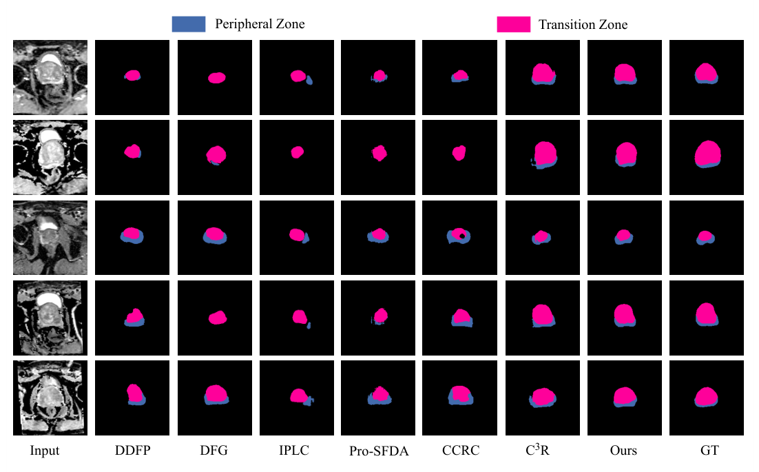
Figure 2 presents representative qualitative comparisons. The visual results show different error patterns across competing methods. DDFP tends to under-segment the prostate, and in some slices it captures only a local part of the TZ. IPLC shows strong inter-slice fluctuation and often produces fragmented foreground predictions, indicating that the pseudo-labels refined by SAM-Med2D are not sufficiently stable in this prostate cross-modality scenario. CCRC occasionally generates anatomically implausible shapes, such as ring-like holes inside the prostate region, while ProSFDA produces overly small predictions with low detection rates in the PZ. DFG performs relatively better among the baselines and can roughly capture the TZ contour, but its ability to delineate the PZ remains limited.
A common issue among competing methods is poor delineation of the peripheral zone. The PZ forms a thin arc-shaped structure surrounding the TZ, and its contrast against adjacent tissues is extremely weak in ADC images. As a result, it is difficult to localize this region from model prediction alone. In contrast, CALM produces segmentation masks that are more consistent with the ground truth: it preserves the overall shape of the TZ and better captures the thin surrounding PZ structure. This qualitative advantage is consistent with the design of CALM, where the population template explicitly encodes the PZ-around-TZ topology and the Soft-AND fusion leverages this group-level prior to generate anatomically more reasonable pseudo-labels.
To further evaluate the generalization ability of CALM beyond the PI-CAI prostate MRI benchmark, we additionally conducted comparative experiments on the abdominal AMOS dataset [31]. As shown in Table 2 and Table 3, CALM achieves the best average DSC and the lowest average ASSD, suggesting that the proposed population template prior and curriculum-guided adaptation strategy are not restricted to a single dataset and can transfer to other anatomically structured segmentation tasks.

4.3. Ablation Study

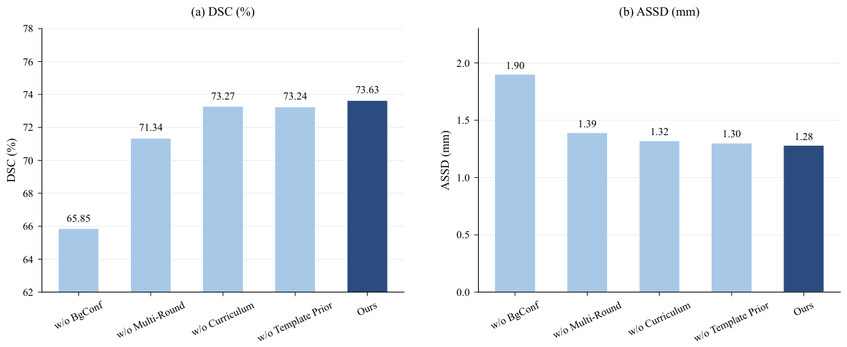
To analyze the contribution of each module in CALM, we perform ablations by removing the population template prior, the high-confidence background constraint (BgConf) in prior-guided pseudo-label learning, the coverage-driven curriculum adaptation, and multi-round adaptation. As shown in Table 4 and Figure 3, the full model achieves the best overall performance, indicating that these components are complementary. Among them, removing BgConf causes the most severe degradation, with average DSC dropping from 73.63% to 65.85% and average ASSD increasing from 1.28 mm to 1.90 mm. This result shows that explicit negative supervision is crucial in prior-guided pseudo-label learning, because without BgConf, false-positive regions can be progressively reinforced during iterative self-training.
Removing multi-round adaptation also leads to a decline in both performance and robustness, reducing the average DSC to 71.34% and increasing its standard deviation from 5.96% to 8.89%. By comparison, removing the population template prior or the coverage-driven curriculum adaptation leads to smaller but still consistent drops, with the average DSC decreasing to 73.24% and 73.27%, respectively. Overall, these results show that CALM benefits from the coordinated effect of the population template prior, BgConf, coverage-driven curriculum adaptation, and multi-round adaptation.

4.4. Model Analysis

4.4.1. Analysis of Module Variants

To further examine the effect of different implementations for key replaceable components in CALM, we compare alternative choices for three submodules: the foreground scoring function in prior-guided pseudo-label learning, the elbow-detection algorithm in coverage-driven curriculum adaptation, and the aggregation rule for class-wise coverage scores. As shown in Table 5, the default product form in Soft-AND fusion achieves the best average DSC of 73.63%, while replacing it with the minimum operator leads to a slight drop to 73.46%, and using the geometric mean causes a larger degradation to 68.03%. This result indicates that element-wise multiplication provides a better balance between the population template prior and instance-specific predictions, whereas the geometric mean is overly sensitive to near-zero probabilities and therefore filters out too many foreground voxels.
For curriculum partitioning, different elbow detection strategies yield highly similar results, with all variants remaining within 0.57 percentage points of each other, suggesting that the distribution of coverage scores can be stably captured by multiple thresholding methods on PI-CAI. A similar trend is observed for coverage aggregation: the default mean and weighted mean perform almost identically, whereas the minimum-based aggregation is slightly inferior, likely because it is too conservative and prematurely excludes samples with low coverage in only one subregion. Based on these observations, we use the product form for Soft-AND fusion, the Kneedle algorithm for elbow detection, and mean aggregation for coverage scoring in the final model.

4.4.2. Hyperparameter Sensitivity Analysis

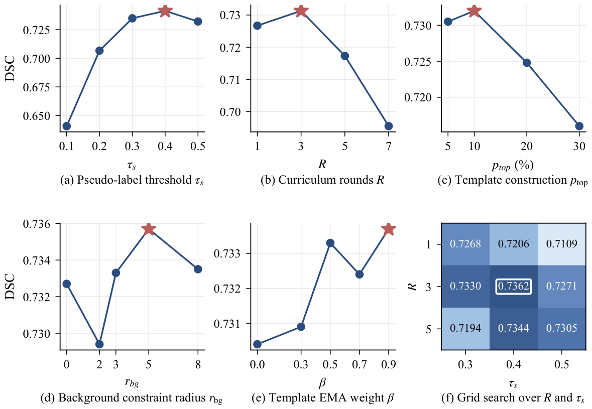
To evaluate the sensitivity of CALM to hyperparameter variations, we analyze the effects of the confidence threshold τ s in prior-guided pseudo-label learning, the number of curriculum rounds in coverage-driven curriculum adaptation, the top-k percentage used in the population template prior, the dilation radius d in BgConf, and the template EMA weight β . As shown in Figure 4a, the best performance is achieved at τ s = 0.4 . When τ s is too small, more low-confidence foreground voxels are retained, which introduces noisy positive supervision into prior-guided pseudo-label learning. In contrast, when τ s becomes too large, many valid foreground voxels are discarded, resulting in insufficient supervision. A similar trade-off can be observed in Figure 4b for the number of curriculum rounds. The best result is obtained with three rounds. With too few rounds, the easy-to-hard adaptation process in coverage-driven curriculum adaptation is not fully exploited. However, when the number of rounds becomes too large, residual pseudo-label noise from difficult samples gradually accumulates and eventually degrades performance.
Figure 4c examines the Top-k percentage in the population template prior. The performance remains stable when the percentage is between 5 % and 10 % , but starts to decline once it exceeds 20 % , because low-quality predictions increasingly dilute the population-level anatomical consensus. When the percentage reaches 50 % , the training process becomes numerically unstable. As shown in Figure 4d and Figure 4e, the dilation radius d in BgConf and the template EMA weight β are much less sensitive, with performance variations of only 0.63 and 0.33 percentage points, respectively. The dilation radius d defines a conservative buffer around the template foreground, excluding ambiguous boundary voxels from high-confidence background supervision. If d is too small, uncertain boundary voxels may be mistaken for reliable background; if it is too large, useful background supervision may be reduced. The default setting d = 5 provides a good balance. The template EMA weight β controls the smoothness of cross-round template updates rather than spatial weighting. A larger β preserves more historical information, whereas a smaller β responds more strongly to current predictions. Finally, Figure 4f presents a 3 × 3 grid search over the two most sensitive hyperparameters, namely τ s and the number of curriculum rounds. The best configuration is achieved at τ s = 0.4 with three rounds, which further validates the default setting adopted in CALM. The heatmap also indicates that these two hyperparameters are not independent, and the optimal performance is obtained only when the strictness of foreground selection and the depth of curriculum adaptation are properly balanced.

4.4.3. Analysis of Curriculum Progression

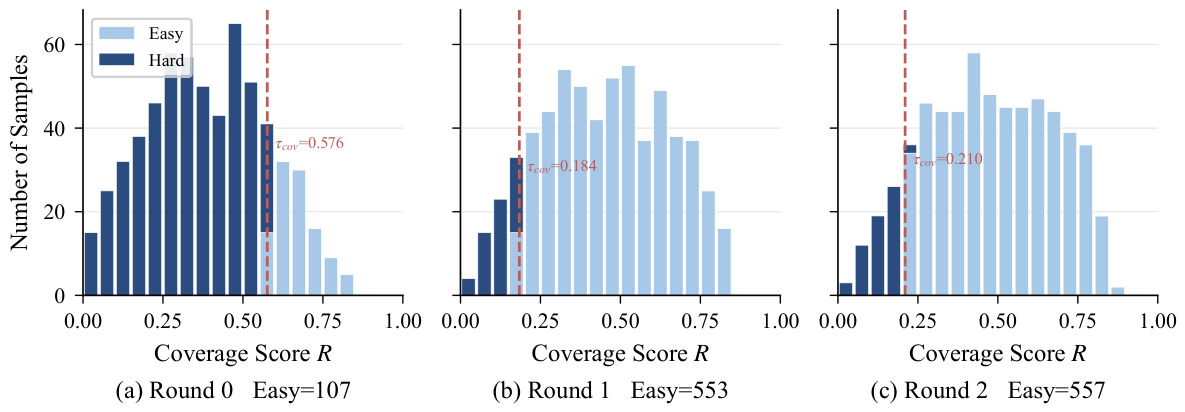
To further understand how the proposed coverage-driven curriculum adaptation works in practice, we analyze the evolution of the easy group across curriculum rounds. As shown in Table 6 and Figure 5, the proportion of samples assigned to the easy group increases progressively from 17.5 % in the first round to 90.2 % and 90.9 % in the subsequent rounds. This trend provides direct evidence that CALM follows the intended easy-to-hard adaptation process: at the beginning, only a small subset of target samples exhibits sufficiently high agreement between pseudo-labels and the population template prior, whereas after iterative refinement, the majority of target samples become reliable enough to participate in self-training. Such a progressive expansion indicates that the curriculum is not a static partition, but an evolving process driven by improvements in pseudo-label quality and template consistency.
Another notable observation is that the easy-group ratio becomes nearly saturated in the final stage, increasing only marginally from 90.2 % to 90.9 % . This suggests that the curriculum gradually approaches convergence after most target samples have been absorbed into the reliable training set. From a methodological perspective, this behavior is consistent with the design of CALM. The population template prior provides a stable structural anchor, prior-guided pseudo-label learning improves supervision quality, and the monotonic growth constraint ensures that once a sample is recognized as reliable, it continues to provide positive supervision in later rounds. Together, these components form a positive feedback loop, through which better templates lead to better pseudo-labels, and better pseudo-labels in turn enlarge the easy group and stabilize the overall adaptation process.

4.5. Computational Overhead and Scalability

To evaluate the computational efficiency of CALM, we compare its overhead with representative SFDA methods. We report the number of parameters, MACs for a single 192 × 192 input, inference latency, peak training GPU memory, and target-adaptation training time. Source-domain pretraining is shared by all methods and is therefore excluded from the training-time comparison.
As shown in Table 7, CALM has 1.81 M parameters and 1.68 G MACs, which is comparable to the lightest baseline and much lower than DFG and SFDA-DDFP. CALM also achieves the lowest inference latency of 0.717 ± 0.006 ms per slice and the lowest peak training memory of 556 MB. The total target-adaptation time of CALM is 13.4 min, which is substantially shorter than the compared SFDA methods. These results indicate that the proposed population-template-guided adaptation strategy improves segmentation performance without introducing heavy computational overhead.
CALM does not modify the segmentation backbone or introduce additional trainable modules. The extra operations, including population template construction, Soft-AND fusion, BgConf selection, and coverage scoring, are performed on voxel-wise probability maps. Therefore, their complexity scales linearly with the number of voxels. For full 3D volumetric datasets with larger spatial resolution, the same operations can be directly applied to 3D probability maps. In practice, memory consumption can be further controlled by patch-wise or sliding-window processing, which is commonly used in high-resolution 3D medical image segmentation.

4.6. Precision Recall Analysis

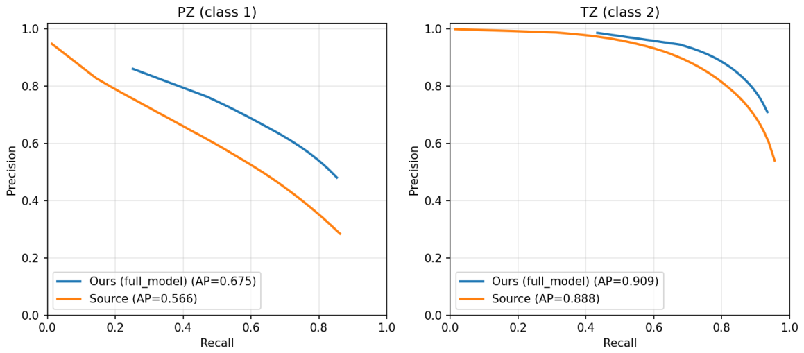
To further analyze the probability-level prediction behavior of CALM, we provide precision recall curves for the two foreground classes, as shown in Figure 6. Compared with the source-only model, CALM shows a better precision–recall trade-off for both PZ and TZ. For the more challenging PZ class, CALM improves the AP from 0.5659 to 0.6748. For the TZ class, CALM also improves the AP from 0.8881 to 0.9093. These results indicate that the proposed adaptation strategy not only improves hard segmentation metrics such as Dice and ASSD, but also enhances the reliability of foreground probability predictions across different decision thresholds.

5. Conclusions and Discussion

In this paper, we present CALM, a source-free domain adaptation framework for cross-modality prostate MRI segmentation. To address unreliable pseudo-label supervision caused by the large discrepancy between T2W and ADC images under the source-free setting, CALM introduces a population template prior to capture target-domain anatomical consensus, a Soft-AND fusion strategy to combine population-level prior knowledge with instance-specific predictions, a high-confidence background constraint to suppress false-positive accumulation, and a coverage-driven curriculum adaptation strategy to progressively expand the reliable training set from easy samples to hard ones. A key technical point is that these components are coupled within one iterative framework, so structural-prior refinement and sample-reliability refinement can improve each other during adaptation.
Clinically, the value of this work is to provide a feasible adaptation path for new target modalities without requiring repeated large-scale manual labeling or source-data access. This may help reduce deployment cost and improve the consistency of prostate subregion delineation in routine workflows.
In future work, we will extend CALM to longitudinal prostate MRI analysis when serial scans from the same patient are available. Although the present study focuses on source-free cross-modality segmentation and does not explicitly model tumor growth dynamics, dynamic propagation models and motion-change analysis methods may provide useful inspiration for extending the current static population template into a spatiotemporal prior [32]. Such an extension would require temporal registration, lesion-level annotations, and longitudinal clinical data, and is therefore left for future studies [33].

Author Contributions

Conceptualization, X.C.; methodology, X.C.; software, X.Z. and Y.W.; validation, X.Z., Y.W., Y.H. and Y.B.; formal analysis, X.C.; investigation, X.C.; writing—original draft preparation, X.Z.; writing—review and editing, X.C.; project administration, X.C. All authors have read and agreed to the published version of the manuscript.

Funding

This work was supported in part by NSFC grant 62276105, Natural Science Foundation of Xiamen, China (3502Z20227193), and Natural Science Foundation of Fujian Province (2023J01136).

Institutional Review Board Statement

Not applicable.

Informed Consent Statement

Not applicable.

Data Availability Statement

The PI-CAI dataset can be accessed publicly at https://pi-cai.grand-challenge.org (accessed on 27 April 2024).

Conflicts of Interest

The authors declare no conflicts of interest.

References

  1. Hamzaoui, D.; Montagne, S.; Renard-Penna, R.; Ayache, N.; Delingette, H. Automatic zonal segmentation of the prostate from 2D and 3D T2-weighted MRI and evaluation for clinical use. J. Med. Imaging 2022, 9, 024001. [Google Scholar] [CrossRef] [PubMed]
  2. Turkbey, B.; Rosenkrantz, A.B.; Haider, M.A.; Padhani, A.R.; Villeirs, G.; Macura, K.J.; Tempany, C.M.; Choyke, P.L.; Cornud, F.; Margolis, D.J.; et al. Prostate Imaging Reporting and Data System Version 2.1: 2019 Update of Prostate Imaging Reporting and Data System Version 2. Eur. Urol. 2019, 76, 340–351. [Google Scholar] [CrossRef] [PubMed]
  3. Wang, R.; Lei, T.; Cui, R.; Zhang, B.; Meng, H.; Nandi, A.K. Medical image segmentation using deep learning: A survey. IET Image Process. 2022, 16, 1243–1267. [Google Scholar] [CrossRef]
  4. Xian, J.; Li, X.L.; Tu, D.; Zhu, S.; Zhang, C.; Liu, X.; Li, X.; Yang, X. Unsupervised Cross-Modality Adaptation via Dual Structural-Oriented Guidance for 3D Medical Image Segmentation. IEEE Trans. Med. Imaging 2023, 42, 1774–1785. [Google Scholar] [CrossRef] [PubMed]
  5. Cabarrus, M.C.; Westphalen, A.C. Multiparametric magnetic resonance imaging of the prostate—A basic tutorial. Transl. Androl. Urol. 2017, 6, 376–386. [Google Scholar] [CrossRef] [PubMed]
  6. Ganin, Y.; Lempitsky, V. Unsupervised domain adaptation by backpropagation. In Proceedings of the 32nd International Conference on Machine Learning, Lille, France, 7–9 July 2015; Volume 37, pp. 1180–1189. [Google Scholar] [CrossRef]
  7. Chen, C.; Liu, Q.; Jin, Y.; Dou, Q.; Heng, P.A. Source-Free Domain Adaptive Fundus Image Segmentation with Denoised Pseudo-Labeling. In Proceedings of the Medical Image Computing and Computer Assisted Intervention–MICCAI 2021; Lecture Notes in Computer Science; Springer: Berlin/Heidelberg, Germany, 2021; Volume 12905, pp. 225–235. [Google Scholar] [CrossRef]
  8. Bateson, M.; Kervadec, H.; Dolz, J.; Lombaert, H.; Ben Ayed, I. Source-free domain adaptation for image segmentation. Med. Image Anal. 2022, 82, 102617. [Google Scholar] [CrossRef] [PubMed]
  9. Zhang, G.; Qi, X.; Yan, B.; Wang, G. IPLC: Iterative pseudo label correction guided by SAM for source-free domain adaptation in medical image segmentation. In Proceedings of the Medical Image Computing and Computer-Assisted Intervention—MICCAI 2024; Springer: Cham, Switzerland, 2024; pp. 351–360. [Google Scholar] [CrossRef]
  10. Yan, F.; Yang, G.; Chen, X.; Yu, Y.; Liu, A. Prior-Guided Selective Parameter Fine-Tuning for Source-Free Domain Adaptive Medical Image Segmentation. IEEE J. Biomed. Health Inform. 2026; early access. [CrossRef] [PubMed]
  11. Ghai, S.; Haider, M.A. Multiparametric-MRI in diagnosis of prostate cancer. Indian J. Urol. 2015, 31, 194–201. [Google Scholar] [CrossRef] [PubMed]
  12. Padgett, K.R.; Swallen, A.; Pirozzi, S.; Piper, J.; Chinea, F.M.; Abramowitz, M.C.; Nelson, A.; Pollack, A.; Stoyanova, R. Towards Universal MRI Atlas of the Prostate and Prostate Zones: Evaluation of Performance between Vendor and Acquisition Parameters. Strahlenther. Und Onkol. 2019, 195, 121–130. [Google Scholar] [CrossRef] [PubMed]
  13. Saha, A.; Bosma, J.S.; Twilt, J.J.; Ginneken, B.V.; Bjartell, A.; Padhani, A.R.; Bonekamp, D.; Villeirs, G.; Salomon, G.; Giannarini, G.; et al. Artificial intelligence and radiologists in prostate cancer detection on MRI (PI-CAI): An international, paired, non-inferiority, confirmatory study. Lancet Oncol. 2024, 25, 879–887. [Google Scholar] [CrossRef] [PubMed]
  14. Liang, J.; Hu, D.; Feng, J. Do we really need to access the source data? Source hypothesis transfer for unsupervised domain adaptation. In Proceedings of the 37th International Conference on Machine Learning, Virtual Event, 13–18 July 2020; Volume 119, pp. 6028–6039. [Google Scholar] [CrossRef]
  15. Yang, C.; Guo, X.; Chen, Z.; Yuan, Y. Source free domain adaptation for medical image segmentation with fourier style mining. Med. Image Anal. 2022, 79, 102457. [Google Scholar] [CrossRef] [PubMed]
  16. Hu, S.; Liao, Z.; Xia, Y. Source-free domain adaptation using prompt learning for medical image segmentation. Pattern Recognit. 2025, 171, 112290. [Google Scholar] [CrossRef]
  17. Yin, S.; Liu, S.; Wang, M. DDFP: Data-dependent frequency prompt for source free domain adaptation of medical image segmentation. Knowl.-Based Syst. 2025, 324, 113651. [Google Scholar] [CrossRef]
  18. Huai, Z.; Tang, H.; Li, Y.; Chen, Z.; Li, X. Leveraging Segment Anything Model for source-free domain adaptation via dual feature guided auto-prompting. IEEE Trans. Med. Imaging 2025, 44, 2618–2631. [Google Scholar] [CrossRef] [PubMed]
  19. Zhang, G.; Qi, X.; Wu, J.; Yan, B.; Wang, G. IPLC+: SAM-guided iterative pseudo label correction for source-free domain adaptation in medical image segmentation. IEEE J. Biomed. Health Inform. 2025, 29, 9060–9072. [Google Scholar] [CrossRef] [PubMed]
  20. Tang, L.; Li, K.; He, C.; Zhang, Y.; Li, X. Source-Free Domain Adaptive Fundus Image Segmentation with Class-Balanced Mean Teacher. In Proceedings of the Medical Image Computing and Computer Assisted Intervention–MICCAI 2023; Greenspan, H., Madabhushi, A., Mousavi, P., Salcudean, S., Duncan, J., Syeda-Mahmood, T., Taylor, R., Eds.; Springer: Cham, Switzerland, 2023; pp. 684–694. [Google Scholar] [CrossRef]
  21. Wang, D.; Shelhamer, E.; Liu, S.; Olshausen, B.; Darrell, T. Tent: Fully test-time adaptation by entropy minimization. In Proceedings of the International Conference on Learning Representations (ICLR), Virtual, 3–7 May 2021. [Google Scholar] [CrossRef]
  22. Wen, Z.; Zhang, X.; Ye, C. Source-free domain adaptation for medical image segmentation via selectively updated mean teacher. In Proceedings of the Information Processing in Medical Imaging—IPMI 2023; Springer: Cham, Switzerland, 2023. [Google Scholar] [CrossRef]
  23. Ma, A.; Zhu, Q.; Li, J.; Nielsen, M.; Chen, X. Source-free domain adaptation for cross-modality cardiac image segmentation with contrastive class relationship consistency. In Proceedings of the Medical Image Computing and Computer-Assisted Intervention—MICCAI 2025; Springer: Berlin/Heidelberg, Germany, 2025; pp. 574–583. [Google Scholar] [CrossRef]
  24. Canny, J. A Computational Approach to Edge Detection. IEEE Trans. Pattern Anal. Mach. Intell. 1986, 8, 679–698. [Google Scholar] [CrossRef] [PubMed]
  25. Tarvainen, A.; Valpola, H. Mean teachers are better role models: Weight-averaged consistency targets improve semi-supervised deep learning results. In Proceedings of the Advances in Neural Information Processing Systems 30 (NeurIPS 2017), Long Beach, CA, USA, 4–9 December 2017; pp. 1195–1204. [Google Scholar] [CrossRef]
  26. Satopaa, V.; Albrecht, J.; Irwin, D.; Raghavan, B. Finding a Kneedle in a Haystack: Detecting Knee Points in System Behavior. In Proceedings of the 2011 31st International Conference on Distributed Computing Systems Workshops; IEEE: Piscataway, NJ, USA, 2011; pp. 166–171. [Google Scholar] [CrossRef]
  27. Ronneberger, O.; Fischer, P.; Brox, T. U-Net: Convolutional Networks for Biomedical Image Segmentation. In Proceedings of the Medical Image Computing and Computer-Assisted Intervention—MICCAI 2015; Springer: Cham, Switzerland, 2015; pp. 234–241. [Google Scholar] [CrossRef]
  28. Ioffe, S.; Szegedy, C. Batch normalization: Accelerating deep network training by reducing internal covariate shift. In Proceedings of the International Conference on Machine Learning (ICML), Lille, France, 7–9 July 2015; pp. 448–456. [Google Scholar] [CrossRef]
  29. Nair, V.; Hinton, G.E. Rectified linear units improve restricted boltzmann machines. In Proceedings of the ICML 2010, Haifa, Israel, 21–24 June 2010; pp. 807–814. [Google Scholar]
  30. Ding, S.; Liu, Z.; Liu, P.; Zhu, W.; Xu, H.; Li, Z.; Niu, H.; Cheng, J.; Liu, T. C3R: Category contrastive adaptation and consistency regularization for cross-modality medical image segmentation. Expert Syst. Appl. 2025, 269, 126304. [Google Scholar] [CrossRef]
  31. Ji, Y.; Bai, H.; Yang, J.; Ge, C.; Zhu, Y.; Zhang, R.; Li, Z.; Zhang, L.; Ma, W.; Wan, X.; et al. AMOS: A Large-Scale Abdominal Multi-Organ Benchmark for Versatile Medical Image Segmentation. arXiv 2022, arXiv:2206.08023. [Google Scholar] [CrossRef]
  32. Meyer, P.G.; Cherstvy, A.G.; Seckler, H.; Hering, R.; Blaum, N.; Jeltsch, F.; Metzler, R. Directedeness, correlations, and daily cycles in springbok motion: From data via stochastic models to movement prediction. Phys. Rev. Res. 2023, 5, 043129. [Google Scholar] [CrossRef]
  33. Muñoz-Gil, G.; Bachimanchi, H.; Pineda, J.; Midtvedt, B.; Fernández-Fernández, G.; Requena, B.; Ahsini, Y.; Asghar, S.; Bae, J.; Barrantes, F.J.; et al. Quantitative evaluation of methods to analyze motion changes in single-particle experiments. Nat. Commun. 2025, 16, 6749. [Google Scholar] [CrossRef] [PubMed]
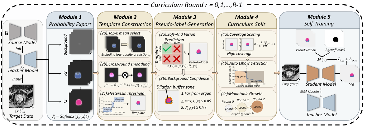
Figure 1. Overview of the proposed CALM framework. Starting from a source-pretrained model and unlabeled target volumes, the teacher model first exports target-domain probability maps. These predictions are used to construct a population template prior through top-k consensus aggregation, cross-round smoothing, and hysteresis thresholding. The template prior is then fused with instance level predictions to generate pseudo-labels and high-confidence background masks. Based on pseudo-label/template consistency, target samples are divided into easy and hard groups for curriculum self-training, and the teacher model is updated by EMA for the next round.
Information 17 00487 g001
Figure 2. Visual comparison of segmentation results of various methods on the PI-CAI dataset.
Information 17 00487 g002
Figure 3. Diagrams of core component ablation on the PI-CAI dataset.
Information 17 00487 g003
Figure 4. Sensitivity analysis of hyperparameters on the PI-CAI dataset. The pentagram marker and the white box indicate the best-performing setting with the highest DSC in the corresponding analysis.
Information 17 00487 g004
Figure 5. Evolution of coverage score distributions across curriculum rounds on the PI-CAI dataset.
Information 17 00487 g005
Figure 6. Precision–recall curves of the source-only model and CALM for PZ and TZ. CALM achieves higher AP values for both foreground classes, especially for the more challenging PZ class.
Information 17 00487 g006
Table 1. Comparison of prostate segmentation performance of different SFDA methods on the PI-CAI dataset, reported as mean ± standard deviation. The best result is highlighted in bold. ** indicates paired t-test p < 0.01 between each baseline and CALM.
MethodDSC (%) ↑ASSD (mm) ↓
PZTZAvg.PZTZAvg.
DDFP15.34 ± 17.52 **31.81 ± 26.52 **23.57 ± 20.97 **21.82 ± 22.92 **14.08 ± 22.01 **17.95 ± 20.84 **
DFG42.93 ± 21.04 **58.98 ± 23.58 **50.95 ± 20.64 **3.70 ± 3.88 **2.73 ± 1.79 **3.22 ± 2.44 **
IPLC16.04 ± 13.34 **63.00 ± 16.07 **39.52 ± 12.32 **19.29 ± 9.26 **4.62 ± 3.75 **11.96 ± 5.86 **
ProSFDA29.45 ± 21.59 **47.60 ± 20.75 **38.52 ± 19.18 **3.76 ± 4.20 **2.92 ± 1.37 **3.34 ± 3.59 **
CCRC30.52 ± 19.10 **44.62 ± 24.83 **37.57 ± 21.05 **5.39 ± 5.81 **4.29 ± 5.19 **4.84 ± 5.87 **
C3R44.98 ± 10.37 **69.59 ± 3.69 **57.28 ± 10.36 **3.91 ± 1.24 **3.68 ± 2.57 **3.80 ± 1.72 **
CALM64.90 ± 8.5582.37 ± 6.4373.63 ± 5.961.41 ± 0.391.16 ± 0.361.28 ± 0.30
Table 2. DSC comparison of abdominal organs segmentation performance of different SFDA methods on the AMOS dataset, reported as mean ± standard deviation. The best result is highlighted in bold. * and ** indicate paired t-test p < 0.05 and p < 0.01 , respectively, between each baseline and CALM.
OrganDSC (%) ↑
DDFPDFGProSFDACCRCIPLCC3RCALM
Spleen62.31 ± 17.95 **23.37 ± 25.31 **28.19 ± 11.64 **59.97 ± 24.03 **72.82 ± 12.5270.22 ± 18.72 **76.40 ± 18.20
Right kidney49.13 ± 22.29 **52.69 ± 33.70 **27.90 ± 11.93 **51.51 ± 32.05 **79.42 ± 14.21 **77.71 ± 13.17 *74.54 ± 16.93
Left kidney30.43 ± 28.77 **41.19 ± 37.51 **1.31 ± 2.48 **53.83 ± 30.63 **77.62 ± 12.31 **75.84 ± 12.84 *70.61 ± 23.32
Gallbladder10.07 ± 26.45 **10.00 ± 30.00 **3.80 ± 18.99 **20.57 ± 27.12 **10.00 ± 30.00 **29.81 ± 23.18 **50.56 ± 29.59
Esophagus37.62 ± 21.13 **25.12 ± 21.91 **0.52 ± 1.26 **4.38 ± 8.16 **0.00 ± 0.00 **49.02 ± 21.66 **57.23 ± 20.03
Liver81.45 ± 7.7853.98 ± 13.63 **55.63 ± 8.24 **81.85 ± 11.2088.33 ± 6.40 **82.58 ± 10.5881.90 ± 10.18
Stomach27.53 ± 20.50 **21.95 ± 22.82 **12.10 ± 7.27 **33.29 ± 24.86 **45.37 ± 15.47 *58.20 ± 21.35 **38.00 ± 27.03
Aorta69.12 ± 16.97 **46.11 ± 24.75 **13.25 ± 11.68 **66.28 ± 22.15 **86.52 ± 10.18 *78.12 ± 8.26 **85.52 ± 9.49
Inferior vena cava38.87 ± 21.42 **33.20 ± 19.36 **19.25 ± 10.40 **16.87 ± 13.22 **63.29 ± 13.90 **64.46 ± 12.21 **71.90 ± 12.23
Pancreas11.36 ± 15.62 **0.18 ± 1.17 **1.33 ± 1.88 **20.97 ± 19.53 **0.00 ± 0.00 **57.50 ± 15.6755.15 ± 16.68
Right adrenal gland0.00 ± 0.00 **0.00 ± 0.00 **0.44 ± 1.32 **2.72 ± 5.30 **0.00 ± 0.00 **31.67 ± 10.3531.67 ± 18.29
Left adrenal gland0.00 ± 0.00 **0.00 ± 0.00 **0.00 ± 0.03 **1.04 ± 3.85 **0.00 ± 0.00 **17.11 ± 12.59 **40.70 ± 20.86
Duodenum18.85 ± 17.23 **1.25 ± 11.11 **0.18 ± 0.37 **7.51 ± 10.41 **1.25 ± 11.11 **40.60 ± 14.53 **44.55 ± 18.34
Average33.60 ± 9.88 **23.77 ± 11.81 **12.61 ± 3.10 **32.37 ± 12.37 **40.36 ± 4.22 **56.37 ± 9.06 **59.90 ± 10.91
Table 3. ASSD comparison of abdominal organs segmentation performance of different SFDA methods on the AMOS dataset, reported as mean ± standard deviation. The best result is highlighted in bold. * and ** indicate paired t-test p < 0.05 and p < 0.01 , respectively, between each baseline and CALM.
OrganASSD (mm) ↓
DDFPDFGProSFDACCRCIPLCC3RCALM
Spleen10.19 ± 4.9515.15 ± 11.75 *18.30 ± 5.58 **13.55 ± 12.4314.67 ± 6.22 **20.95 ± 16.92 **10.99 ± 9.33
Right kidney22.09 ± 9.0612.09 ± 13.04 **13.33 ± 6.15 **15.14 ± 20.28 **12.04 ± 7.87 **5.39 ± 3.39 **21.89 ± 9.81
Left kidney38.14 ± 19.73 **11.09 ± 16.5329.38 ± 18.37 **15.40 ± 15.21 **12.22 ± 7.53 **5.57 ± 4.08 *8.39 ± 9.27
Gallbladder25.37 ± 22.68 **-45.96 ± 29.74 **20.80 ± 37.53 *-27.36 ± 17.96 **13.88 ± 25.16
Esophagus9.41 ± 17.54 **6.79 ± 4.52 **46.72 ± 20.95 **12.43 ± 7.52 **-3.98 ± 3.403.79 ± 3.39
Liver6.36 ± 3.86 **21.39 ± 5.60 **18.60 ± 5.17 **7.97 ± 4.73 **4.72 ± 3.17 **10.41 ± 7.5712.27 ± 6.36
Stomach17.28 ± 9.44 **20.27 ± 13.82 **21.03 ± 6.78 **14.74 ± 13.0422.71 ± 6.08 **15.44 ± 10.4512.97 ± 10.65
Aorta5.11 ± 4.79 **16.61 ± 11.56 **16.48 ± 4.88 **4.81 ± 4.30 **2.33 ± 2.663.12 ± 2.88 **2.47 ± 2.83
Inferior vena cava8.88 ± 5.51 **9.41 ± 7.14 **8.50 ± 2.73 **15.84 ± 12.38 **4.40 ± 2.98 **3.99 ± 3.033.56 ± 2.12
Pancreas22.24 ± 17.15 **21.67 ± 3.95 **27.38 ± 6.79 **12.28 ± 9.61 **-6.26 ± 4.346.17 ± 3.98
Right adrenal gland--25.90 ± 15.38 **6.86 ± 3.71-9.23 ± 7.49 **6.16 ± 5.30
Left adrenal gland--47.38 ± 25.09 **8.03 ± 3.37 *-15.34 ± 7.44 **4.53 ± 5.33
Duodenum26.30 ± 33.73 **-27.75 ± 14.61 **17.05 ± 11.45 **-8.69 ± 6.11 **6.54 ± 5.35
Average17.12 ± 7.44 **14.83 ± 7.95 **25.97 ± 5.78 **13.84 ± 8.51 **10.41 ± 3.53 **10.44 ± 4.25 **8.72 ± 4.20
Table 4. Results of core component ablation on PI-CAI dataset.
MethodDSC (%) ↑ASSD (mm) ↓ΔDSC
PZTZAvg.PZTZAvg.
w/o BgConf60.03 ± 8.6971.68 ± 12.0765.85 ± 8.491.73 ± 0.472.06 ± 0.821.90 ± 0.53−7.78
w/o Multi-Round62.54 ± 10.3880.14 ± 10.2871.34 ± 8.891.49 ± 0.601.28 ± 0.561.39 ± 0.50−2.29
w/o Curriculum64.46 ± 8.9082.08 ± 6.5073.27 ± 6.231.47 ± 0.391.17 ± 0.371.32 ± 0.32−0.36
w/o Template Prior64.53 ± 7.2481.95 ± 6.9073.24 ± 5.431.39 ± 0.351.20 ± 0.451.30 ± 0.31−0.39
Ours64.90 ± 8.5582.37 ± 6.4373.63 ± 5.961.41 ± 0.391.16 ± 0.361.28 ± 0.30
Table 5. Results of the ablation study on module variants on the PI-CAI dataset.
SubmoduleVariantPZ DSC (%)TZ DSC (%)Avg. (%)ΔDSC
Fusion scoringprod (default)64.90 ± 8.5382.37 ± 6.4273.63 ± 5.95-
min65.00 ± 7.6681.92 ± 6.5173.46 ± 5.61−0.17
gmean59.10 ± 8.6876.97 ± 8.9268.03 ± 7.30−5.60
Elbow detectionkneedle (default)64.90 ± 8.5382.37 ± 6.4273.63 ± 5.95-
diff65.01 ± 8.4082.08 ± 6.4973.54 ± 6.05−0.09
otsu64.90 ± 8.4782.09 ± 6.4973.49 ± 5.98−0.14
second64.29 ± 8.9981.82 ± 7.1573.06 ± 6.72−0.57
Coverage aggregationmean (default)64.90 ± 8.5382.37 ± 6.4273.63 ± 5.95-
weighted_mean64.81 ± 8.4482.32 ± 5.9473.57 ± 5.74−0.06
min64.39 ± 8.4381.77 ± 7.1073.08 ± 6.27−0.55
Table 6. Progressive curriculum learning process on the PI-CAI dataset.
RoundEasy CasesHard CasesEasy RatioτcovDSCΔDSC
010750617.5%0.5760.7260-
15536090.2%0.1840.7406+0.0146
25575690.9%0.2100.7431+0.0025
Final test DSC (after Round 2):73.63%
Table 7. Computational overhead on PI-CAI. We report the number of parameters, MACs for a single 192 × 192 forward pass, inference latency, peak training GPU memory, and total target-adaptation training time. Source-domain pretraining is shared across all methods and is excluded.
MethodParams (M)MACs (G)Latency (ms)Train Mem (MB)Train Time (min)
Ours (CALM)1.811.68 0.717 ± 0.006 55613.4
SFDA-CCRC6.553.76 2.091 ± 0.016 794124.2
SFDA-DDFP31.0430.80 1.875 ± 0.037 1823241.3
IPLC1.811.74 0.929 ± 0.016 843250.2
DFG31.0430.75 1.843 ± 0.003 2063110.8
ProSFDA22.014.56 1.546 ± 0.011 1104609.4
Disclaimer/Publisher’s Note: The statements, opinions and data contained in all publications are solely those of the individual author(s) and contributor(s) and not of MDPI and/or the editor(s). MDPI and/or the editor(s) disclaim responsibility for any injury to people or property resulting from any ideas, methods, instructions or products referred to in the content.