Article

On Segment-Aware Monocular Depth Estimation Using Vision Transformers

by
Vasileios Arampatzakis
1,2,*,
George Pavlidis
2,
Nikolaos Mitianoudis
1 and
Nikos Papamarkos
1
1
Department of Electrical and Computer Engineering, Democritus University of Thrace, 67100 Xanthi, Greece
2
Athena Research Center, 67100 Xanthi, Greece
*
Author to whom correspondence should be addressed.
Information 2026, 17(2), 145; https://doi.org/10.3390/info17020145
Submission received: 23 December 2025 / Revised: 16 January 2026 / Accepted: 22 January 2026 / Published: 2 February 2026

Abstract

Monocular Depth Estimation (MDE) infers per-pixel scene geometry from a single RGB image. Despite recent progress, global MDE models often blur depth discontinuities at object boundaries and fail to capture object-level structure. Segment-aware depth estimation addresses this limitation by exploiting semantic segmentation to decompose depth prediction into simpler, class-specific subproblems. In this work, we study semantic-aware MDE in a multi-branch design where each semantic class is handled by a lightweight Vision Transformer (ViT) branch that predicts dense depth for its class while suppressing interference from other regions. We further examine fusion strategies that merge the branch outputs into a single prediction: (i) a learnable cross-attention fusion module that predicts depth from the stack of per-class proposals and masks, and (ii) a parameter-free stitched summation that sums mask-gated outputs. The proposed architecture is simple, scalable, end-to-end trainable, and compatible with arbitrary transformer backbones. Experiments on Virtual KITTI 2, where ground-truth depth and semantic labels are available, show that segment-aware modeling produces sharper depth boundaries and improves standard error metrics compared to a single-branch baseline (AbsRel 0.243→0.152; RMSE 11.952→9.101). Finally, we find that the parameter-free summation matches, and in most cases improves upon, the accuracy of learned fusion while adding no computational overhead.

1. Introduction

Accurate depth estimation from a single image is crucial for autonomous driving, robotics, and 3D scene reconstruction. Modern MDE models rely on convolutional or transformer networks trained on large RGB-D datasets. Most of these models treat depth estimation as a global pixel-wise regression task, which often leads to blurred object boundaries and loss of local detail. Depth and semantics are closely related: boundaries between semantic objects typically coincide with depth discontinuities, and the depth distribution within a segment tends to follow class-specific patterns. Recent work demonstrates that incorporating segmentation cues can improve MDE. For example, SHED uses a bidirectional segment hierarchy to inform depth prediction [1], and Jiao et al. introduce an attention-driven synergy network where semantic features are shared with depth estimation [2]. However, these methods typically learn segmentation jointly with depth or inject semantic cues into a single predictor; comparatively little work studies the simpler alternative of training class-specific depth experts given external masks and then composing their outputs.
This paper investigates a segment-aware architecture for MDE. Given an image, its semantic masks, and the corresponding depth map during training, we train one depth branch per semantic class so that each branch specialises on a narrow semantic domain. At inference time, we assume that semantic masks are provided by an external segmentation system. Crucially, we study how to compose the class-wise depth proposals into a single prediction: (i) a learnable cross-attention fusion module that directly predicts depth from the stack of per-class proposals and masks, and (ii) a parameter-free stitched summation that simply sums the mask-gated per-class predictions (our proposed default, since it adds no computational overhead). An overview of the baseline and the two segment-aware variants is shown in Figure 1.
In this work we focus on settings where such masks are accurate, as in Virtual KITTI 2 [3,4], in order to isolate and quantify the benefit of segment-wise depth decomposition. Our goal is not to compete with the latest large-scale, multi-dataset depth systems, but to answer a more focused architectural question: given the same backbone, optimiser, and training set, does explicit segment-wise decomposition improve depth quality compared to a purely global predictor? To keep this question well-posed, all of our quantitative comparisons are carried out against a single-branch baseline trained under identical data, optimiser, and training recipe (using the same compact encoder–decoder design as each expert branch), rather than against external monocular depth models that benefit from substantially larger backbones and pretraining corpora. In that stronger regime, our segment-aware decomposition would act as a mechanism for combining class-wise experts (with optional learned fusion), but such experiments would conflate the effects of semantics with gains due to model scale and pretraining and are therefore left outside the scope of this paper. The proposed segment-aware design is explicitly backbone-agnostic: in principle, each expert branch could be replaced by any off-the-shelf depth module, including state-of-the-art predictors trained on external data. Our contributions are as follows:
  • Segment-aware depth experts with transformers. We propose a multi-branch monocular depth architecture in which each semantic class is handled by a dedicated, compact ViT encoder–decoder expert that receives a mask-gated RGB input and predicts a dense depth proposal for that class.
  • Two composition strategies (learned vs. parameter-free). We study how to compose per-class depth proposals into a single prediction by comparing (i) a cross-attention fusion module that directly predicts depth from the stack of per-class proposals and masks, and (ii) a parameter-free stitched summation that sums the mask-gated proposals.
  • Controlled study with accuracy–efficiency trade-offs. Under a controlled training protocol (same data, optimiser, and per-branch backbone) on Virtual KITTI 2, we evaluate 3-, 6-, and 11-class schemes and quantify both accuracy and computational cost. We find that most gains come from the segment-wise decomposition, while simple summation is a strong default that is competitive with, and often outperforms, learned fusion without additional overhead.
To the best of our knowledge, the closest prior work that decomposes monocular depth prediction into category-wise experts conditioned on explicit segments is the Semantic Divide-and-Conquer (SDC-Depth) network [5]. SDC-Depth decomposes the scene into panoptic segments and predicts a canonical depth map for each segment; segments of the same category share a decoder, and scale/shift parameters are estimated to reconstruct the global depth. Our approach differs in three key ways: (i) we use precomputed masks rather than predicting segmentation, (ii) we assign a separate encoder–decoder to each class instead of sharing decoders across categories, and (iii) we study both a learnable cross-attention fusion module and a parameter-free summation baseline, rather than relying on category-wise scale/shift regression. PanopticDepth [6], a closely related model, predicts depth per instance using instance-specific convolution kernels and merges them into a panoptic map. In contrast, our model operates on semantic classes (not instances) and composes class-wise outputs via attention or parameter-free summation rather than dynamic convolutions.

2. Related Work

2.1. Monocular Depth Estimation

Deep networks have greatly advanced monocular depth estimation [7]. Early convolutional architectures regress pixel-wise depth from an RGB image; examples include the Deep Ordinal Regression Network (DORN) [8], which casts depth estimation as an ordinal regression problem and discretises the depth range into intervals, and MiDaS [9], which mixes multiple datasets to learn robust, scale-invariant depth predictors. Transformer-based models further improve global context aggregation by modelling long-range dependencies and have recently achieved state-of-the-art results. Self-supervised and self-training methods exploit photometric consistency across stereo pairs or video frames to supervise depth when ground-truth is unavailable, reducing dependence on dense RGB-D datasets. Despite these advances, most global models still treat depth estimation as a purely pixel-wise regression problem and tend to blur object boundaries or under-utilise semantic structure.

2.2. Semantic Guidance for Depth Estimation

Semantic information can provide strong priors for depth estimation [10]. SDC-Depth [5] decomposes each scene into panoptic segments and predicts a canonical, scale- and shift-invariant depth map for each category, reassembling them via learned scale and shift parameters. PanopticDepth [6] proposes a unified framework for depth-aware panoptic segmentation, where dynamic convolution kernels predict instance-wise masks and depth maps, enabling instance-specific context sharing between segmentation and depth. SHED [1] redesigns the vision transformer to use hierarchical segment tokens that are pooled and unpooled across encoder and decoder layers, jointly reasoning about coarse-to-fine semantics and depth. The Semantic-aware Spatial Feature Alignment (SSFA) framework of Li et al. [11] aligns implicit semantic features with depth features and adds a semantic-guided ranking loss, showing that guiding depth with semantics can improve both metric and relative depth accuracy. Unlike these joint or implicit approaches, our method assumes that semantic masks are provided and trains separate depth experts per semantic class, composing their outputs either via cross-attention fusion or via a parameter-free summation.
An early example of explicitly conditioning depth on semantics is the work of Ladický et al. [12], who couple semantic labels and depth in a unified structured prediction framework to encourage semantic and geometric consistency. Their formulation effectively exploits class-conditioned depth priors, anticipating later divide-and-conquer strategies. Our segment-aware architecture can be seen as a modern, end-to-end analogue: we similarly exploit class-wise structure, but replace hand-crafted features and Conditional Random Field (CRF) fusion with transformer-based per-class experts and a modular composition stage (cross-attention fusion or parameter-free summation). More recently, ROIFormer [13] proposes a semantic-aware region-of-interest transformer for self-supervised monocular depth estimation, constraining cross-attention to local regions guided by semantic cues. In contrast, ROIFormer operates in a self-supervised, real-world setting with a single depth predictor whose attention is restricted by semantics, whereas our model allocates distinct transformer branches to each semantic class and fuses their depth proposals at the output level in a fully supervised synthetic setup on Virtual KITTI 2. A detailed quantitative comparison with these methods would require different training regimes and datasets and is therefore beyond the scope of this work.

2.3. Depth Refinement with Masks

Mask-guided depth refinement treats segmentation as a post-processing cue. Kim et al. [14] introduced Layered Depth Refinement with Mask Guidance, a framework that decomposes an initial depth map into foreground and background layers using a binary or soft mask and performs separate inpainting and outpainting operations to refine depth boundaries. Their approach relies on high-quality masks and refines the output of an existing depth estimator rather than learning depth from scratch. In contrast, our method integrates segmentation cues directly into the estimation pipeline, exploiting mask information during both training and inference to produce sharper boundaries and semantically consistent depth predictions.
Saeedan and Roth [15] similarly use panoptic segmentation maps to boost self-supervised monocular depth estimation via panoptic-guided smoothing, alignment, and stereo consistency losses. Their method regularises a single depth network using instance-level masks, while our approach integrates semantic masks at the architectural level by training per-class depth experts and fusing their outputs. We view these panoptic-guided losses as complementary to our segment-aware design, but a detailed comparison on real-world self-supervised benchmarks is outside the scope of this paper, which focuses on fully supervised depth estimation on Virtual KITTI 2.
In summary, prior work has either jointly learned depth and segmentation in a single network, injected semantic features into a global depth predictor, or used semantic and panoptic masks to regularise self-supervised losses. To the best of our knowledge, prior work has not systematically studied this setting with precomputed semantic masks and separate transformer-based depth experts per class under a controlled protocol with the same training recipe and per-branch backbone, while also contrasting learned cross-attention fusion against a parameter-free stitched summation. Figure 1 provides a high-level schematic of the baseline, the segment-aware model with learned fusion, and the segment-aware no-fusion stitched summation.

3. Segment-Aware Depth Estimation

3.1. Preliminaries

Let I ∈ R 3 × H × W be an RGB image, D ∈ R 1 × H × W its metric depth map, and M ∈ { 0 , 1 } N × H × W the binary semantic masks, where N is the number of classes. We assume M is exclusive on the set of valid pixels, i.e., at most one class is active per pixel. In our Virtual KITTI 2 setup we treat the Sky class as invalid: Sky pixels are excluded from all losses and metrics, and the corresponding mask entries are set to zero. Hence, for non-Sky pixels we have ∑ i = 1 N M i ( p ) = 1 , while for Sky pixels ∑ i = 1 N M i ( p ) = 0 . Each class map M i is a binary mask that activates pixels belonging to that class.

3.2. Per-Class Depth Branches

Each class has a dedicated depth branch built from a small Vision Transformer encoder followed by a convolutional decoder. Given I and M i , we form the masked input I i = I ⊙ M i . The encoder processes I i and outputs token features, which the decoder upsamples back to an H × W map. We apply a softplus activation to ensure positive depth and obtain an unmasked per-class depth proposal:
z i = σ f i I ⊙ M i ,
where f i denotes the encoder–decoder of branch i and σ is the softplus nonlinearity, ensuring positive depths. Each z i is multiplied by its corresponding mask M i when composing the stitched depth by summation, so that predictions are gated outside the class region.

3.3. Cross-Attention Fusion

We form a stitched depth map via mask-gated summation of the per-class predictions:
z sum = ∑ i = 1 N M i ⊙ z i .
On valid (non-Sky) pixels, where ∑ i M i ( p ) = 1 , this summation is equivalent to the mask-weighted average and simply selects the unique active class prediction at each pixel. On Sky pixels, all masks are zero and the pixel is ignored by the losses/metrics. Therefore, at semantic boundaries the stitched depth transitions by switching the contributing expert pixel-wise (hard routing); overlaps do not occur and gaps arise only on invalid Sky pixels, which are excluded from training and evaluation.
The learnable fusion module replaces this fixed stitching with a lightweight cross-attention network that directly predicts the final depth map z from { z i , M i } i = 1 N . We first compute two global summary maps: the mean mask m mean = 1 N ∑ i M i and a scale-sensitive cue given by the per-pixel standard deviation σ z = Std i M i ⊙ z i across the masked per-class depth maps. We deliberately restrict these fusion cues to low-dimensional, easily interpretable statistics to keep the fusion module lightweight and to avoid conflating our main contribution (segment-wise depth experts) with an aggressively engineered fusion mechanism. We then patchify these maps by average pooling to a coarse grid of H c × W c patches (patch size 16 × 16 , a fixed non-tuned choice consistent with common ViT practice) and flatten them into tokens, trading off fusion spatial granularity against computational cost.
The query tokens are obtained by linearly projecting the two-channel token sequence [ m mean , σ z ] . Keys and values are obtained by concatenating the depth-mask stack [ z 1 , M 1 , … , z N , M N ] , patchifying it in the same way, and projecting the resulting 2 N -channel tokens. A stack of transformer-style cross-attention blocks updates the queries given the fixed keys/values. Finally, the updated query tokens are reshaped back to the H c × W c grid, bilinearly upsampled to H × W , and passed through a small convolutional head to regress the fused depth map:
z = σ g ( F ( { z i , M i } i = 1 N ) ) ,
where F ( · ) denotes the fusion pipeline (patchification and projection of inputs, cross-attention updates, token-to-grid reshaping, and upsampling to H × W ). Here, g ( · ) denotes the convolutional regression head and σ ( · ) is the softplus nonlinearity enforcing positive depth. Unlike residual “refinement” formulations, the fusion module predicts z directly. Exploring alternative aggregation cues (e.g., probabilistic gating or confidence-weighted mixtures) is a natural extension, but we leave it to future work to preserve the controlled scope of this study.

3.4. Losses

Following Eigen et al. [16], we use the scale-invariant log RMSE (SI-RMSE) for metric depth. The global depth loss is SI-RMSE plus a small BerHu term [17] (weight 0.02 ); during the first 5 epochs we warm up with ℓ 1 instead of SI-RMSE + BerHu. To encourage within-object smoothness, we add an edge-aware regulariser weighted by image gradients (weight 1 × 10 − 2 ). During training we sum the global depth loss with an epoch-weighted sum of per-branch SI-RMSE losses computed on each semantic class mask M i (no BerHu per branch). Sky pixels are excluded by construction (their mask entries are set to zero), and we skip a branch loss if a batch contains no pixels for that class. Because Virtual KITTI 2 provides ground-truth semantic labels and we do not learn a segmentation head, there is no segmentation loss term; the fusion model is trained end-to-end purely from depth supervision. Concretely, the total training objective is
L = L global + W seg ∑ i = 1 N L SI ( i ) + λ smooth L smooth ,
where L global is the global SI-RMSE+BerHu loss on the fused depth, L SI ( i ) is the SI-RMSE for branch i on class mask M i , computed only if the batch contains pixels of class i, W seg is the epoch-dependent segment loss weight, and λ smooth is the edge-aware smoothness weight. In all experiments we use a two-stage schedule for the segment-loss weight: W seg = 0.25 for epochs 1–5 (warm-up) and W seg = 0.15 for epochs 6–50, applied identically across all variants and class schemes.

3.5. No-Fusion Variant

To isolate the contribution of the cross-attention module, we experiment with a no-fusion model where the per-class depths are summed without refinement. Concretely, we remove the fusion module and treat the stitched summation as the final prediction, i.e., z = z sum = ∑ i = 1 N ( M i ⊙ z i ) .

4. Experimental Setup

4.1. Dataset

We evaluate on the Virtual KITTI 2 dataset [3,4], which provides synthetic driving scenes with RGB images, 16-bit depth maps (values in centimetres), and per-pixel semantic labels. Images are resized to 256 × 256, and the dataset is split into 90% training and 10% validation sets (a commonly used split, kept fixed across all variants and not treated as a tunable hyperparameter). Concretely, we recursively collect all matched (RGB, depth, semantic) triplets, shuffle them at the frame level with a fixed seed, and assign the first 90% to training and the remaining 10% to validation (i.e., the split is not scene-disjoint, consistent with our goal of a controlled architectural comparison). Our conclusions are comparative and are drawn under an identical fixed-seed split and training recipe for all variants to isolate architectural differences under the same empirical evaluation protocol, while scene-/sequence-disjoint generalisation is a complementary question beyond the scope of this study. Semantic labels are remapped into 3, 6, and 11 classes according to three segmentation schemes used in our experiments. These schemes capture coarse, mid-level, and fine semantic granularity:
  • 3-class: Vegetation = {Tree, Vegetation}; Ground = {Road, Terrain}; Artificial = {Building, Truck, Car, Van, GuardRail, TrafficSign, TrafficLight, Pole, Misc}.
  • 6-class: Road = {Road}; Terrain = {Terrain}; Building = {Building}; Vegetation = {Tree, Vegetation}; Object = {GuardRail, TrafficSign, TrafficLight, Pole, Misc}; Vehicle = {Truck, Van, Car}.
  • 11-class: Terrain, Tree, Vegetation, Building, Road, GuardRail, TrafficSign, TrafficLight, Pole, Misc, Vehicle = {Truck, Car, Van}.
Due to severe class imbalance among vehicle subclasses (Truck and Van jointly account for less than 2% of pixels), training separate experts for each vehicle category led to unstable Truck predictions. We therefore merge Truck, Car, and Van into a single Vehicle class in the 11-class configuration.

4.2. Model Variants

  • Baseline: a single ViT encoder-decoder that predicts depth from RGB only, without access to semantic masks.
  • Segment-aware (Fusion): per-class experts (one encoder–decoder per semantic class), followed by a cross-attention fusion module. The fusion module takes the stack of per-class depth maps and their masks as input and directly predicts a fused depth map.
  • Segment-aware (No-Fusion)—proposed: per-class experts (one encoder–decoder per semantic class); the class-wise predictions are mask-gated and summed to form the final depth, with no additional fusion or refinement.
All three variants share the same compact encoder–decoder backbone and are trained from scratch on Virtual KITTI 2. This controlled setup ensures that our comparisons isolate the contribution of the segment-aware decomposition and fusion, rather than the choice of backbone or external training data. We intentionally define the baseline as the single expert “unit” and evaluate segment-aware models as parallel compositions of the same unit across classes; thus, the increased parameters/FLOPs are an explicit accuracy–efficiency trade-off (see the complexity analysis in Section 5.2), rather than an uncontrolled confound. For this reason we deliberately refrain from including large pre-trained depth systems as “external baselines”: they would almost certainly achieve lower absolute error on Virtual KITTI 2, but such a comparison would answer a different question (which model has the largest pre-training budget) rather than whether semantics help a fixed backbone.
For closely related semantic-aware pipelines such as SDC-Depth [5] and PanopticDepth [6], a fair quantitative comparison on our split would require retraining their full pipelines under the same compact from-scratch recipe and aligning their additional assumptions (e.g., panoptic/instance inputs, scale-shift reconstruction, or dynamic kernels). Since our goal is to isolate the architectural effect of segment-wise decomposition (experts + composition) rather than to re-benchmark heterogeneous training regimes, we restrict quantitative evaluation to the controlled baseline and variants described above.

4.3. Training Details

All models are trained on Virtual KITTI 2 at 256 × 256 resolution for 50 epochs using the AdamW optimizer with a cosine-annealing learning rate schedule, shared across all variants. We use 50 epochs and a single, standard AdamW + cosine training recipe as fixed (non-tuned) hyperparameters, applied uniformly across all variants to avoid confounding the architectural comparison with optimisation choices. For all configurations we use a batch size of 4. The learning rate is set to 5 × 10 − 4 with weight decay 10 − 4 ; the loss schedule follows ℓ 1 warm-up for the first five epochs and the SI-RMSE+BerHu objective thereafter. All results are obtained on a single NVIDIA GPU using these shared hyperparameters. For stability we apply gradient clipping with a maximum norm of 1.0. Each expert branch uses a compact ViT encoder with patch size 16 × 16 , embedding dimension 128, depth 2 transformer blocks, and 4 attention heads (MLP ratio 4 and dropout 0.1), followed by a lightweight convolutional decoder that reshapes tokens to an H / 16 × W / 16 grid, upsamples to H × W via bilinear interpolation, applies two 3 × 3 convolutions (128→64→32) with GELU, and uses a final 1 × 1 head with softplus output to regress positive metric depth. No data augmentation is used beyond resizing inputs to 256 × 256 (no random crops, flips, or photometric transforms).

4.4. Evaluation Metrics

We evaluate on valid pixels (all classes except Sky). Let d i and d ^ i denote ground-truth and predicted depth at valid pixel i, and let N be the number of valid pixels. We report the following:
  • Absolute Relative Error (AbsRel): AbsRel = 1 N ∑ i = 1 N | d i − d ^ i | d i .
  • Squared Relative Error (SqRel): SqRel = 1 N ∑ i = 1 N ( d i − d ^ i ) 2 d i .
  • Root Mean Squared Error (RMSE): RMSE = 1 N ∑ i = 1 N ( d i − d ^ i ) 2 .
  • Log RMSE (RMSElog): RMSE log = 1 N ∑ i = 1 N ( log d i − log d ^ i ) 2 .
  • Threshold accuracy  ( δ k ) : δ k = 1 N i : max d ^ i d i , d i d ^ i < 1 . 25 k ,   k ∈ { 1 , 2 , 3 } .

5. Results

5.1. Accuracy Results

Across all class schemes, segment-wise decomposition is the dominant source of improvement. As reported in Table 1 (validation on Virtual KITTI 2 excluding Sky pixels), both segment-aware variants outperform the single-branch baseline on every metric. When selecting a default model, we prioritise absolute depth accuracy (RMSE, SqRel): the parameter-free stitched summation is consistently the best and also the most efficient. The learned fusion module mainly improves the strict threshold accuracy δ 1 , indicating better relative agreement on many pixels, but this does not always translate into lower squared absolute error.
Because the baseline does not use semantic masks, it is unaffected by mask perturbations. Under mask noise, both segment-aware variants degrade as expected; stitched summation is more sensitive to hard routing errors, while fusion degrades more gracefully on the reported indicators (Table 2). We observed the same qualitative trend under stronger boundary perturbations (e.g., r = 2).
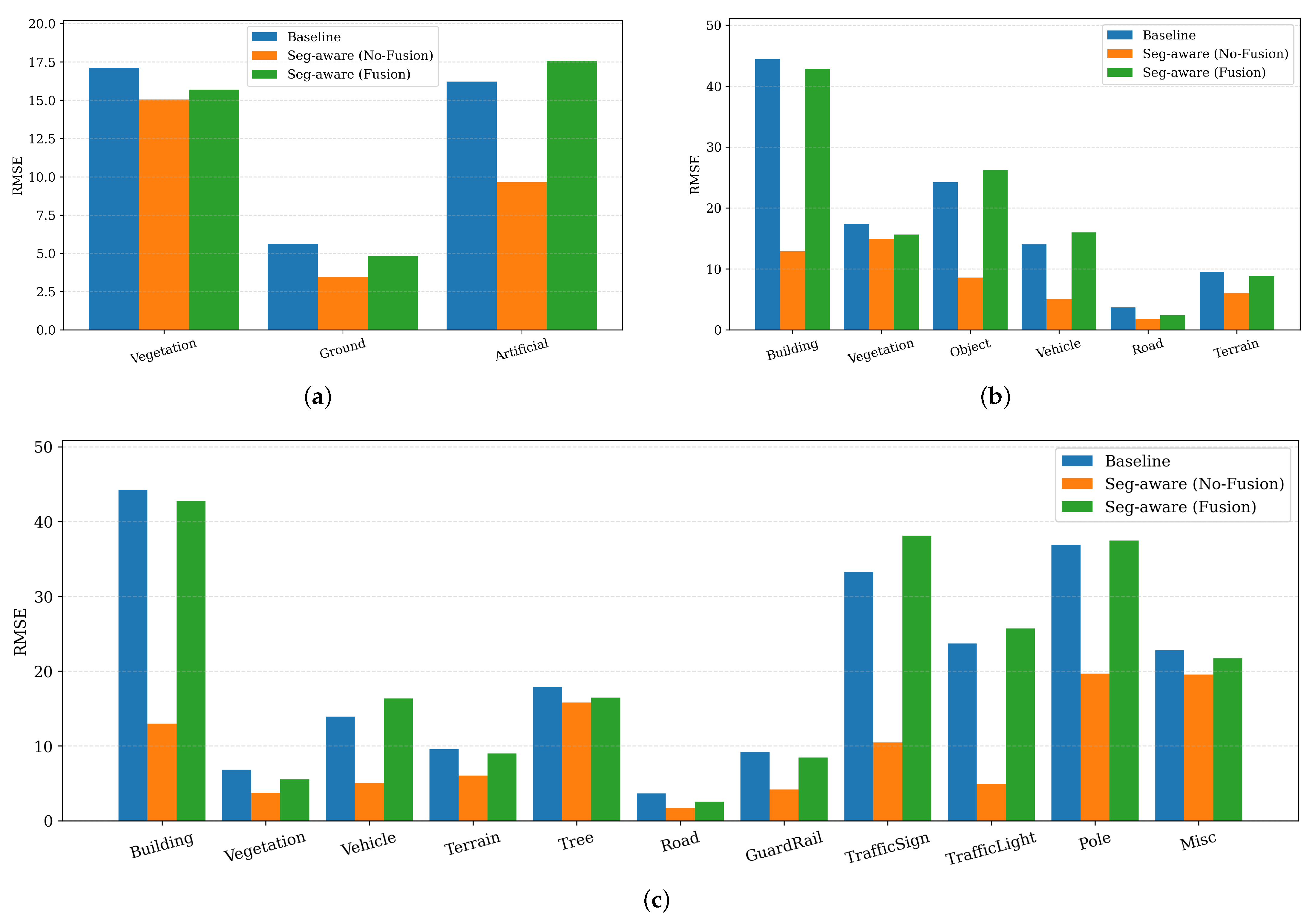
A class-wise breakdown in Figure 2 supports the same conclusion. Stitched summation is the most reliable composition for absolute depth accuracy: it consistently reduces per-class RMSE and achieves the best global RMSE/SqRel with zero overhead. In contrast, learned fusion offers a modest gain in δ 1 but is less stable across categories and can introduce larger errors in specific classes.
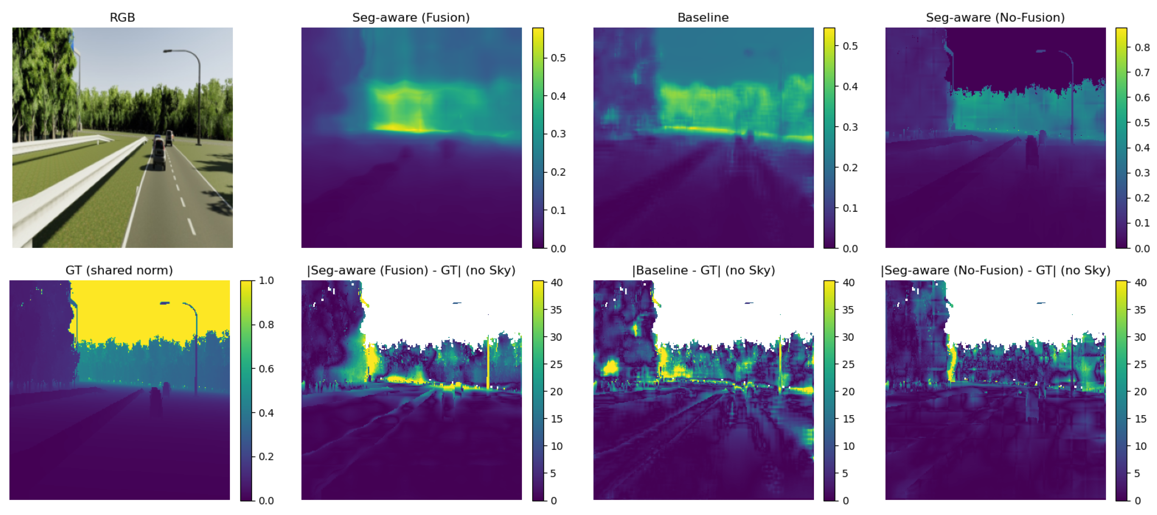
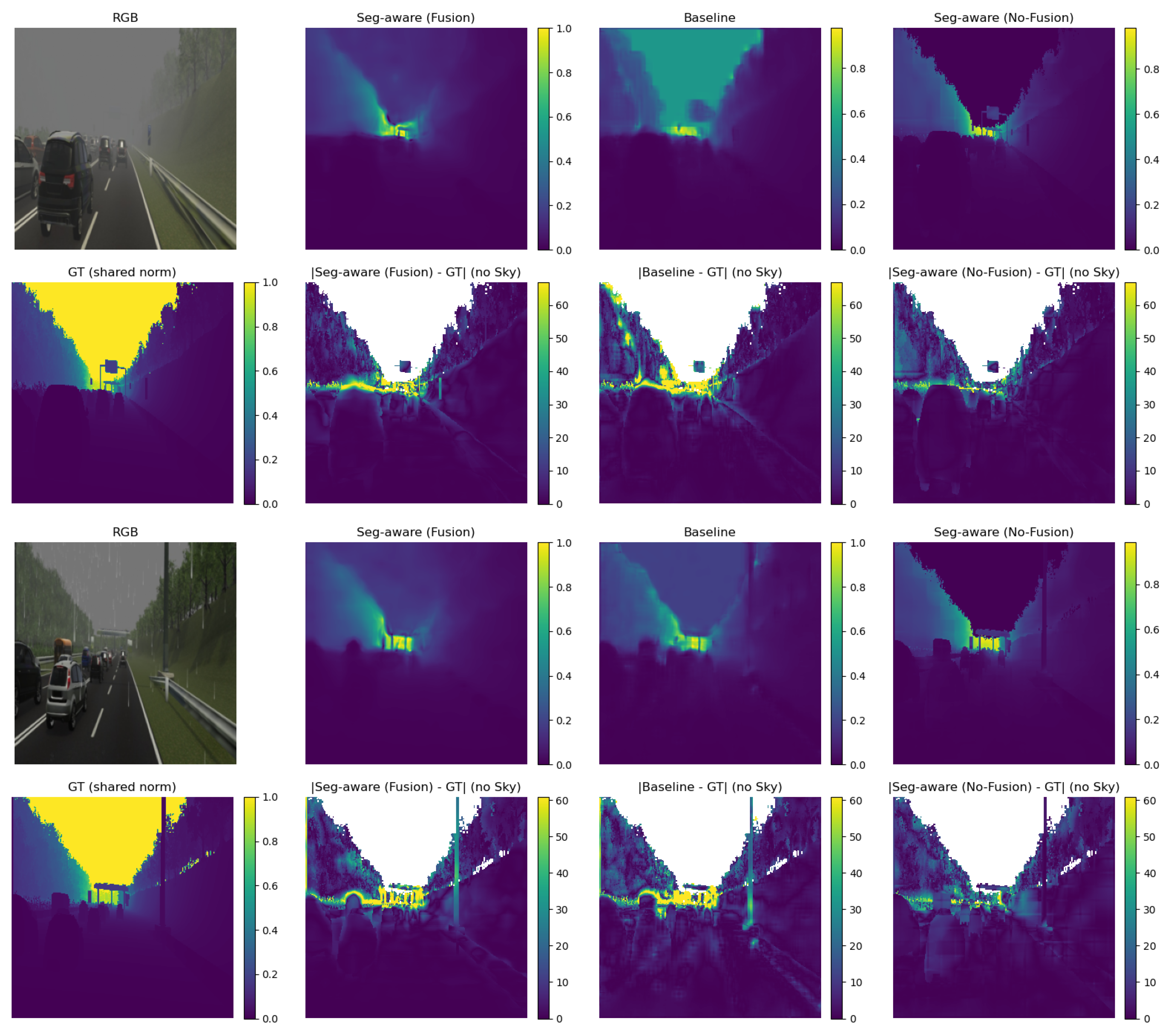
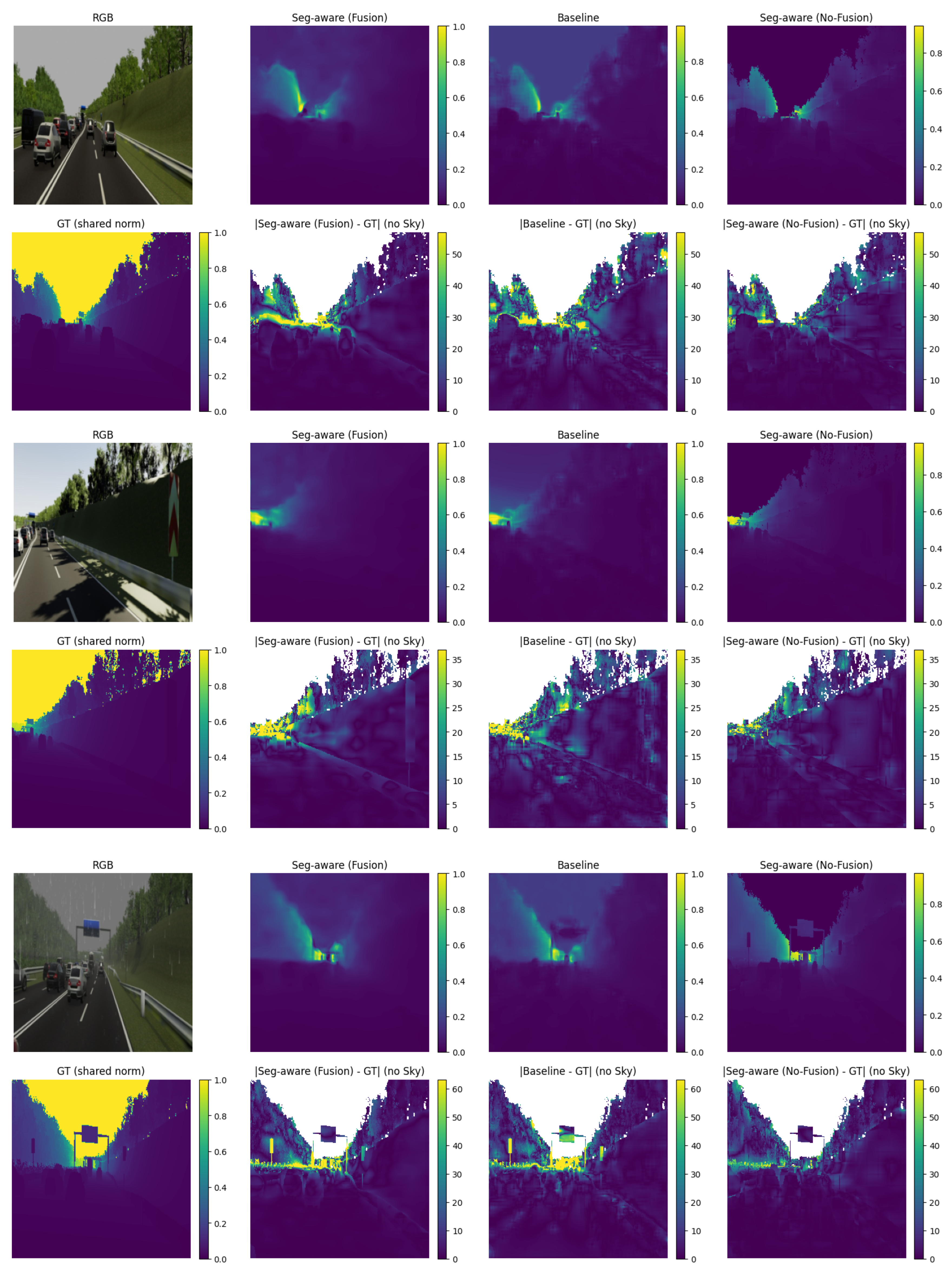
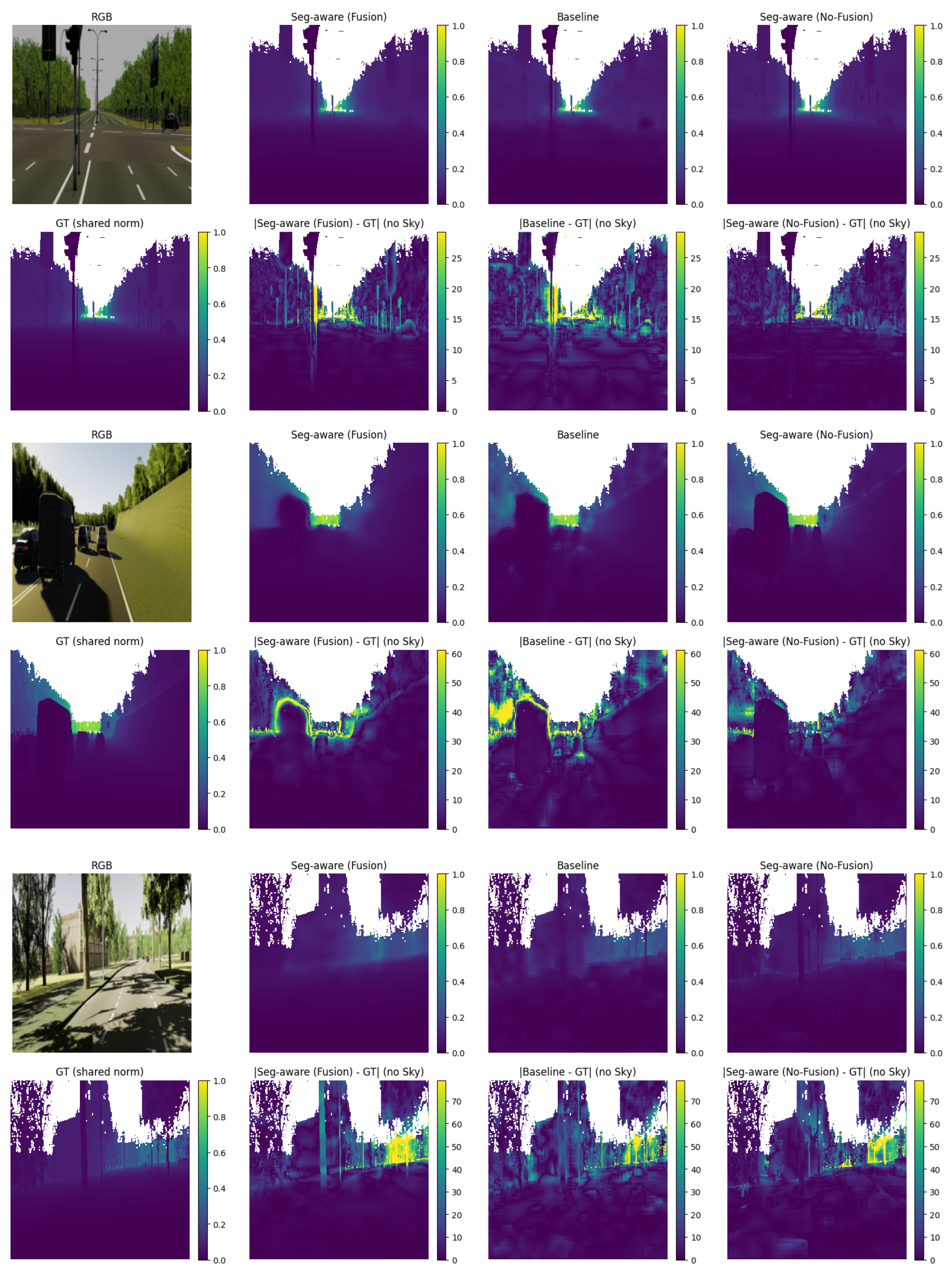
Qualitative comparisons are shown in Figure 3, Figure 4 and Figure 5 for the 3-, 6-, and 11-class schemes, respectively. Relative to the baseline, both segment-aware variants tend to preserve sharper depth discontinuities aligned with semantic boundaries, reducing leakage across adjacent regions. The absolute-error maps (computed excluding Sky pixels) show lower error in many areas; however, fusion can occasionally introduce local deviations, consistent with the per-class RMSE trends in Figure 2.

5.2. Model Complexity and Runtime

To characterise the computational cost of the proposed architecture, Table 3 reports parameter counts and Floating-Point operations (FLOPs) per 256 × 256 image for the baseline and the segment-aware variants. For real-time considerations, we report inference cost in FLOPs (hardware-independent) relative to the single-branch baseline. The results show that model size and FLOPs grow approximately linearly with the number of semantic classes, reflecting the one-branch-per-class design. Even the largest 11-class configuration remains below 8M parameters. Compared to stitched summation, the fusion variant adds additional parameters and computation. In our implementation, most of this cost is driven by the patch-token grid and the attention blocks, while the input projection introduces a smaller dependence on the number of semantic classes N. This quantifies the trade-off: parameter-free summation is the most efficient variant, while learned fusion incurs moderate extra computation that may improve accuracy for some metrics.

6. Discussion

Our experiments isolate a simple architectural question: given accurate semantic masks, does decomposing monocular depth estimation into class-specific experts improve depth quality relative to a single global predictor trained under the same data and optimisation, and is a learned fusion stage necessary? Across all segmentation schemes, the answer to the first part is consistently positive. Both segment-aware variants improve the baseline on the full suite of standard metrics in Table 1, and the qualitative examples in Figure 3, Figure 4 and Figure 5 show noticeably sharper depth discontinuities at semantic boundaries.
Where the gains come from. The per-class design reduces interference between unrelated regions (e.g., vegetation vs. road vs. vehicles) by restricting each branch to a narrower appearance–geometry distribution. This is reflected in the per-class RMSE bars in Figure 2, where stitched summation (No-Fusion) reduces error for most categories compared to the baseline. The qualitative panels further support this interpretation: boundary leakage visible in the baseline is typically reduced when predictions are produced by class-specific experts and gated by the corresponding masks.
Learned fusion vs. stitched summation. The second part of the question is more nuanced. While the fusion module can improve strict threshold accuracy (most clearly δ 1 ), it is not consistently better on absolute error metrics such as RMSE and SqRel. In our controlled setting, the parameter-free stitched summation is the most reliable composition for absolute accuracy: it achieves the lowest RMSE/SqRel for the 3- and 6-class schemes, and the best overall relative/log error profile (AbsRel, SqRel, RMSElog) for the 11-class scheme (Table 1). This supports the practical recommendation stated in the abstract: stitched summation is a strong default that matches, and in most cases improves upon, learned fusion without adding computational overhead. Our goal is to compare composition rules under a shared objective and fixed recipe, and the same qualitative pattern across the 3/6/11-class schemes supports stitched summation as the most reliable default for absolute-error criteria (RMSE/SqRel) overall, while fusion most consistently benefits δ 1 .
One plausible reason for this behaviour is that the fusion head is trained to regress depth directly from stacked proposals at a coarse patch resolution and may trade small, widespread improvements in relative agreement for occasional larger deviations in depth magnitude. This pattern is visible in the class-wise trends: fusion can be competitive on boundary-sensitive criteria ( δ 1 ), yet can yield worse RMSE for specific categories (Figure 2). Importantly, our qualitative visualisations mask Sky consistently and use shared scales within each sample, so the observed differences are not artefacts of per-image normalisation.
Accuracy–efficiency trade-off. The complexity results in Table 3 show that the one-branch-per-class design scales approximately linearly with the number of classes. The stitched summation variant adds no parameters beyond the experts and requires only a mask-gated sum, whereas learned fusion introduces additional attention and convolutional layers. Given that summation is also the most stable option for RMSE/SqRel, this efficiency profile strengthens its role as the default choice when absolute depth accuracy and runtime are the primary constraints.
Limitations and scope. This study uses ground-truth semantic labels from Virtual KITTI 2 to isolate the effect of segment-wise decomposition under accurate masks. In real deployments, masks will be predicted and therefore imperfect; to probe sensitivity to imperfect masks without retraining, we additionally perform an inference-only stress test by perturbing the ground-truth masks at test time via erosion/dilation (r = 1 px) and random label flips (p = 0.03) (Table 2). As expected, boundary misalignment and small-region errors act primarily as hard routing noise for stitched summation (No-Fusion), causing leakage across adjacent classes near object boundaries, while class confusion routes pixels to the wrong expert and introduces larger inconsistencies. The fusion variant is more tolerant to these perturbations because it can blend competing proposals using disagreement cues, though severe mask errors can still degrade performance since the per-class proposals are themselves mask-conditioned. A broader robustness study with predicted masks from external segmenters (e.g., Mask R-CNN or SAM) remains an important next step and is left for future work. We do not evaluate on real-world datasets (e.g., KITTI or NYU-Depth V2) to keep the analysis focused on isolating the effect of segment-wise decomposition under reliable masks; real-world validation with predicted masks is left for future work. In addition, our experts are intentionally lightweight and trained from scratch on a single synthetic dataset. Because the design is backbone-agnostic, a promising direction is to instantiate each branch with stronger depth backbones (including pretrained models) and study the interaction between semantic decomposition and model scale. An additional direction is to constrain learned fusion to operate as a bounded residual correction on top of stitched summation (instead of predicting depth directly), which may reduce occasional large deviations while retaining the strong RMSE/SqRel behaviour and efficiency of summation.

7. Conclusions

We studied segment-aware monocular depth estimation as a controlled architectural intervention: instead of a single global predictor, depth is estimated by lightweight class-specific ViT experts whose outputs are composed into a final depth map. On Virtual KITTI 2, segment-aware modelling consistently improves standard depth metrics over a single-branch baseline trained under the same data, optimiser, and training recipe and produces qualitatively sharper discontinuities at semantic boundaries. Quantitatively, our best segment-aware configuration improves AbsRel from 0.243 to 0.152 and RMSE from 11.952 to 9.101 on Virtual KITTI 2.
A central finding is that the simplest composition rule is also a strong performer. The parameter-free stitched summation of mask-gated expert predictions matches, and in most cases improves upon, a learned cross-attention fusion module on the key absolute error criteria (RMSE, SqRel), while adding no computational overhead. Learned fusion can provide modest gains in strict threshold accuracy ( δ 1 ), but it is less stable class-wise and does not reliably reduce squared absolute error.
Overall, these results suggest a practical recipe: use segment-wise decomposition to obtain sharper boundaries and better accuracy, and adopt stitched summation as the default fusion strategy; enable learned fusion only when threshold accuracy is the primary target. A key limitation of this study is that it assumes accurate semantic masks and uses a multi-expert design whose compute scales with the number of classes; future work will evaluate robustness under predicted/noisy masks and explore more efficient variants (e.g., shared encoders with class-specific heads), as well as extend the framework to stronger backbones and real-world datasets.

Author Contributions

Conceptualization, V.A., G.P., N.M., and N.P.; methodology, V.A. and G.P.; software, V.A.; validation, V.A. and G.P.; formal analysis, V.A. and G.P.; investigation, V.A.; resources, G.P., N.M., and N.P.; data curation, V.A.; writing—original draft preparation, V.A.; writing—review and editing, V.A., G.P., N.M., and N.P.; visualization, V.A.; supervision, G.P., N.M., and N.P.; project administration, N.P.; funding acquisition, G.P. All authors have read and agreed to the published version of the manuscript.

Funding

This research was funded by the European Union’s Horizon Europe programme under grant agreement No 101132308 (ARGUS-Non-destructive, scalable, smart monitoring of remote cultural treasures).

Institutional Review Board Statement

Not applicable.

Informed Consent Statement

Not applicable.

Data Availability Statement

The Virtual KITTI 2 dataset used in this study is publicly available.

Acknowledgments

During the preparation of this manuscript/study, the author used ChatGPT (OpenAI; model: GPT-5.2 Thinking) for English language phrasing.

Conflicts of Interest

The author declares no conflicts of interest. The funders had no role in the design of the study; in the collection, analyses, or interpretation of data; in the writing of the manuscript; or in the decision to publish the results.

References

  1. Lee, S.H.; Mo, S.; Yu, S.X. SHED Light on Segmentation for Depth Estimation. In Proceedings of the Structural Priors for Vision Workshop at ICCV’25, Honolulu, HI, USA, 19 October 2025. [Google Scholar]
  2. Jiao, J.; Cao, Y.; Song, Y.; Lau, R. Look Deeper into Depth: Monocular Depth Estimation with Semantic Booster and Attention-Driven Loss. In Proceedings of the European Conference on Computer Vision (ECCV), Munich, Germany, 8–14 September 2018. [Google Scholar]
  3. Cabon, Y.; Murray, N.; Humenberger, M. Virtual KITTI 2. arXiv 2020, arXiv:2001.10773. [Google Scholar] [CrossRef] [Scilit]
  4. Gaidon, A.; Wang, Q.; Cabon, Y.; Vig, E. Virtual worlds as proxy for multi-object tracking analysis. In Proceedings of the IEEE conference on Computer Vision and Pattern Recognition, Las Vegas, NV, USA, 26 June–1 July 2016; pp. 4340–4349. [Google Scholar]
  5. Wang, L.; Zhang, J.; Wang, O.; Lin, Z.; Lu, H. SDC-Depth: Semantic Divide-and-Conquer Network for Monocular Depth Estimation. In Proceedings of the IEEE/CVF Conference on Computer Vision and Pattern Recognition (CVPR), Seattle, WA, USA, 14–19 June 2020. [Google Scholar]
  6. Gao, N.; He, F.; Jia, J.; Shan, Y.; Zhang, H.; Zhao, X.; Huang, K. PanopticDepth: A Unified Framework for Depth-Aware Panoptic Segmentation. In Proceedings of the IEEE/CVF Conference on Computer Vision and Pattern Recognition (CVPR), New Orleans, LA, USA, 18–24 June 2022; pp. 1632–1642. [Google Scholar]
  7. Arampatzakis, V.; Pavlidis, G.; Mitianoudis, N.; Papamarkos, N. Monocular Depth Estimation: A Thorough Review. IEEE Trans. Pattern Anal. Mach. Intell. 2024, 46, 2396–2414. [Google Scholar] [CrossRef] [Scilit]
  8. Fu, H.; Gong, M.; Wang, C.; Batmanghelich, K.; Tao, D. Deep Ordinal Regression Network for Monocular Depth Estimation. In Proceedings of the IEEE Conference on Computer Vision and Pattern Recognition (CVPR), Salt Lake City, UT, USA, 18–22 June 2018. [Google Scholar]
  9. Ranftl, R.; Lasinger, K.; Hafner, D.; Schindler, K.; Koltun, V. Towards Robust Monocular Depth Estimation: Mixing Datasets for Zero-Shot Cross-Dataset Transfer. IEEE Trans. Pattern Anal. Mach. Intell. 2022, 44, 1623–1637. [Google Scholar] [CrossRef] [Scilit] [PubMed]
  10. Chen, P.Y.; Liu, A.H.; Liu, Y.C.; Wang, Y.C.F. Towards Scene Understanding: Unsupervised Monocular Depth Estimation with Semantic-Aware Representation. In Proceedings of the IEEE/CVF Conference on Computer Vision and Pattern Recognition (CVPR), Long Beach, CA, USA, 16–20 June 2019. [Google Scholar]
  11. Li, R.; Xue, D.; Su, S.; He, X.; Mao, Q.; Zhu, Y.; Sun, J.; Zhang, Y. Learning depth via leveraging semantics: Self-supervised monocular depth estimation with both implicit and explicit semantic guidance. Pattern Recognit. 2023, 137, 109297. [Google Scholar] [CrossRef] [Scilit]
  12. Ladicky, L.; Shi, J.; Pollefeys, M. Pulling Things out of Perspective. In Proceedings of the IEEE Conference on Computer Vision and Pattern Recognition (CVPR), Columbus, OH, USA, 23–28 June 2014. [Google Scholar]
  13. Xing, D.; Shen, J.; Ho, C.; Tzes, A. ROIFormer: Semantic-Aware Region of Interest Transformer for Efficient Self-Supervised Monocular Depth Estimation. Proc. AAAI Conf. Artif. Intell. 2023, 37, 2983–2991. [Google Scholar] [CrossRef] [Scilit]
  14. Kim, S.Y.; Zhang, J.; Niklaus, S.; Fan, Y.; Chen, S.; Lin, Z.; Kim, M. Layered Depth Refinement with Mask Guidance. In Proceedings of the IEEE/CVF Conference on Computer Vision and Pattern Recognition (CVPR), New Orleans, LA, USA, 18–24 June 2022; pp. 3855–3865. [Google Scholar]
  15. Saeedan, F.; Roth, S. Boosting Monocular Depth with Panoptic Segmentation Maps. In Proceedings of the IEEE/CVF Winter Conference on Applications of Computer Vision (WACV), Virtual, 5–9 January 2021; pp. 3853–3862. [Google Scholar]
  16. Eigen, D.; Puhrsch, C.; Fergus, R. Depth Map Prediction from a Single Image using a Multi-Scale Deep Network. In Proceedings of the 28th International Conference on Neural Information Processing Systems; Ghahramani, Z., Welling, M., Cortes, C., Lawrence, N., Weinberger, K., Eds.; Curran Associates, Inc.: Red Hook, NY, USA, 2014; Volume 27. [Google Scholar]
  17. Laina, I.; Rupprecht, C.; Belagiannis, V.; Tombari, F.; Navab, N. Deeper Depth Prediction with Fully Convolutional Residual Networks. In Proceedings of the 2016 Fourth International Conference on 3D Vision (3DV), Stanford, CA, USA, 25–28 October 2016; pp. 239–248. [Google Scholar] [CrossRef] [Scilit]
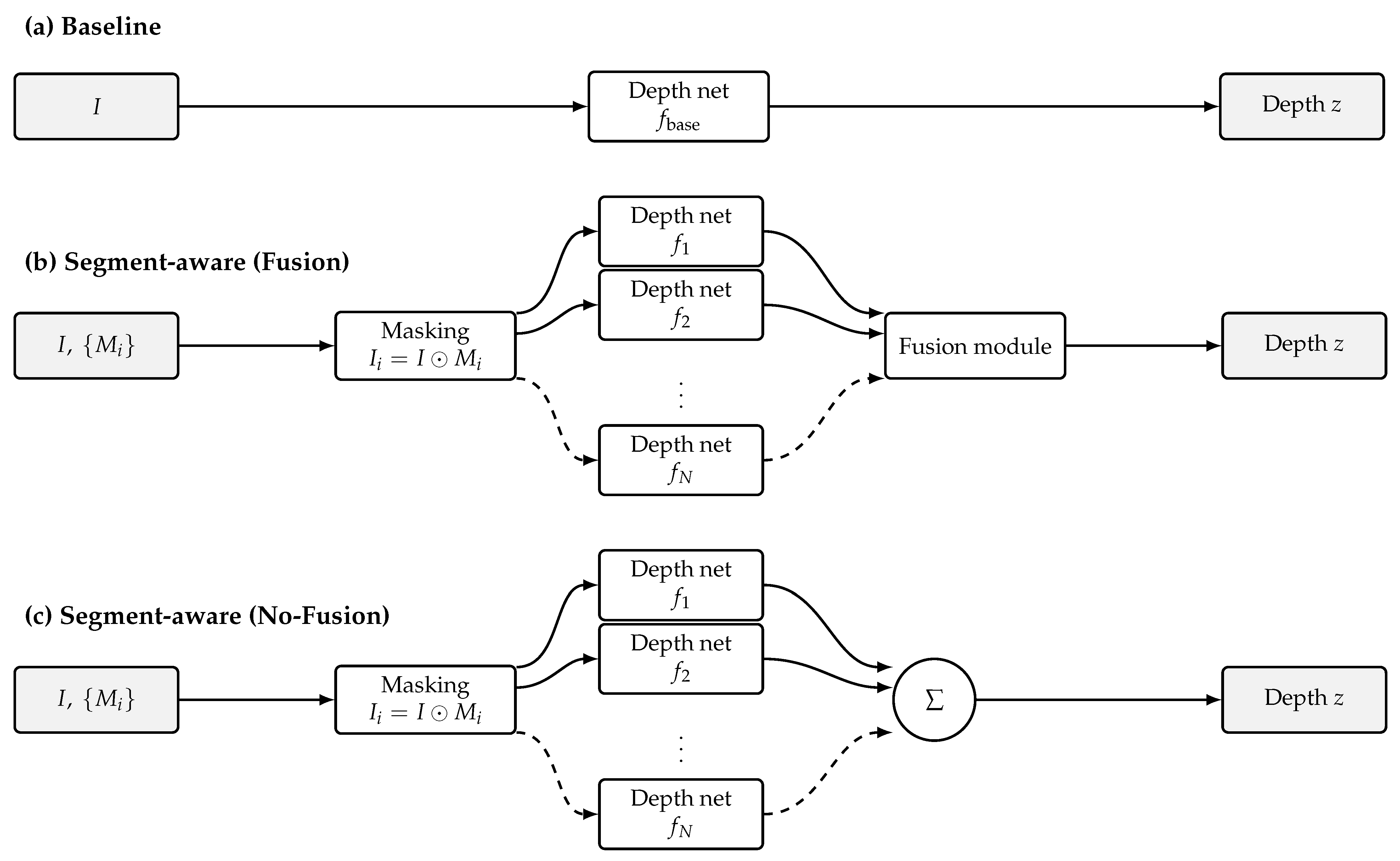
Figure 1. Overview of the three monocular depth pipelines: (a) baseline, (b) segment-aware with cross-attention fusion, and (c) segment-aware without fusion.
Information 17 00145 g001
Figure 2. Per-class RMSE on Virtual KITTI 2 shown as bar charts. Subplots (a–c) correspond to the 3-, 6-, and 11-class schemes, respectively. For each semantic class, the grouped bars report RMSE for the Baseline, Segment-aware (No-Fusion), and Segment-aware (Fusion) models.
Information 17 00145 g002
Figure 3. Qualitative results on Virtual KITTI 2 (3-class scheme). Each panel shows one sample as a 2 × 4 grid. Top row (left to right): RGB input, Segment-aware (Fusion) prediction, Baseline prediction, and Segment-aware (No-Fusion) prediction. Bottom row: normalised ground-truth depth (Sky masked in white) and the corresponding absolute error maps for Fusion, Baseline, and No-Fusion, computed excluding Sky-class pixels. Depth maps are normalised to [ 0 , 1 ] using a shared ground-truth-derived scale per sample; error maps show absolute error in meters on a shared linear scale within each sample.
Information 17 00145 g003aInformation 17 00145 g003b
Figure 4. Qualitative results on Virtual KITTI 2 (6-class scheme). Each panel shows one sample as a 2 × 4 grid. Top row (left to right): RGB input, Segment-aware (Fusion) prediction, Baseline prediction, and Segment-aware (No-Fusion) prediction. Bottom row: normalised ground-truth depth (Sky masked in white) and the corresponding absolute error maps for Fusion, Baseline, and No-Fusion, computed excluding Sky-class pixels. Depth maps are normalised to [ 0 , 1 ] using a shared ground-truth-derived scale per sample; error maps show absolute error in meters on a shared linear scale within each sample.
Information 17 00145 g004
Figure 5. Qualitative results on Virtual KITTI 2 (11-class scheme). Each panel shows one sample as a 2 × 4 grid. Top row (left to right): RGB input, Segment-aware (Fusion) prediction, Baseline prediction, and Segment-aware (No-Fusion) prediction. Bottom row: normalised ground-truth depth (Sky masked in white) and the corresponding absolute error maps for Fusion, Baseline, and No-Fusion, computed excluding Sky-class pixels. Depth maps are normalised to [ 0 , 1 ] using a shared ground-truth-derived scale per sample; error maps show absolute error in meters on a shared linear scale within each sample.
Information 17 00145 g005
Table 1. Quantitative results on the Virtual KITTI 2 dataset, evaluated on all classes except Sky. Lower values indicate better error performance; higher values indicate better accuracy. Bold values indicate the best overall result per evaluation metric across all reported models.
ModelClassesAbsRelSqRelRMSERMSE_log δ 1 δ 2 δ 3
Baseline-0.2433.76211.9520.2970.6840.8940.957
Segment-aware (Fusion)30.1533.09011.1530.2300.8410.9450.975
Segment-aware (No-Fusion)30.1852.2599.5470.2370.7640.9260.972
Segment-aware (Fusion)60.1553.14611.1770.2270.8440.9460.975
Segment-aware (No-Fusion)60.1561.9089.1010.2070.8090.9440.980
Segment-aware (Fusion)110.1623.25211.3040.2350.8280.9410.974
Segment-aware (No-Fusion)110.1521.8959.2500.2040.8130.9460.981
Table 2. Inference-only mask robustness stress test on Virtual KITTI 2 validation (11-class scheme). We perturb semantic masks at test time via morphological erosion/dilation (radius r = 1 px) and random label flips (p = 0.03). Baseline does not use masks and is unchanged. Bold values indicate the best result per evaluation metric for each perturbation condition.
ConditionModelAbsRel δ 1
cleanBaseline0.23590.6889
cleanNo-Fusion0.14190.8314
cleanFusion0.15970.8281
erode (r = 1)No-Fusion0.16580.8029
erode (r = 1)Fusion0.16490.8185
dilate (r = 1)No-Fusion0.21590.7462
dilate (r = 1)Fusion0.18420.8099
flip (p = 0.03)No-Fusion0.29600.7522
flip (p = 0.03)Fusion0.17780.7927
Table 3. Model complexity on Virtual KITTI 2 at 256 × 256 resolution. Params denotes the number of trainable parameters and FLOPs are the approximate multiply–add operations per forward pass.
ModelClassesParams (M)FLOPs (G)
Baseline-0.916.88
Segment-aware (Fusion)32.8538.04
Segment-aware (No-Fusion)31.7618.50
Segment-aware (Fusion)64.6256.55
Segment-aware (No-Fusion)63.5237.01
Segment-aware (Fusion)117.5587.39
Segment-aware (No-Fusion)116.4667.85
Disclaimer/Publisher’s Note: The statements, opinions and data contained in all publications are solely those of the individual author(s) and contributor(s) and not of MDPI and/or the editor(s). MDPI and/or the editor(s) disclaim responsibility for any injury to people or property resulting from any ideas, methods, instructions or products referred to in the content.