BWO-Optimized CNN-BiGRU-Attention Model for Short-Term Load Forecasting

Abstract

Short-term load forecasting is essential for optimizing power system operations and supporting renewable energy integration. However, accurately capturing the complex nonlinear features in load data remains challenging. To improve forecasting accuracy, this paper proposes a hybrid CNN-BiGRU-Attention model optimized by the Beluga Whale Optimization (BWO) algorithm. The proposed method integrates deep learning with metaheuristic optimization in four steps: First, a Convolutional Neural Network (CNN) is used to extract spatial features from input data, including historical load and weather variables. Second, a Bidirectional Gated Recurrent Unit (BiGRU) network is employed to learn temporal dependencies from both forward and backward directions. Third, an Attention mechanism is introduced to focus on key features and reduce the influence of redundant information. Finally, the BWO algorithm is applied to automatically optimize the model’s hyperparameters, avoiding the problem of falling into local optima. Comparative experiments against five baseline models (BP, GRU, BiGRU, BiGRU-Attention, and CNN-BiGRU-Attention) demonstrate the effectiveness of the proposed model. The experimental results indicate that the optimized model achieves superior predictive performance with significantly reduced error rates in terms of Mean Absolute Percentage Error (MAPE) and Root Mean Square Error (RMSE), along with a higher Coefficient of Determination ($R^2$) compared to the benchmarks, confirming its high accuracy and reliability for power load forecasting.

1. Introduction

In the era of smart grids, the rapid proliferation of distributed renewable energy resources has introduced significant volatility to power systems [1]. Consequently, short-term electricity load forecasting has become a cornerstone for ensuring grid stability, optimizing economic dispatch, and formulating efficient generation schedules. Unlike stable baseloads, modern electricity consumption patterns are increasingly stochastic, driven by complex interactions between meteorological conditions (e.g., temperature and precipitation), multi-scale temporal periodicities, and dynamic social behaviors [2]. This complexity necessitates forecasting models that possess both high precision and robustness.

Traditional approaches to this problem have generally bifurcated into physical and statistical methodologies. Physical models, while grounded in thermodynamic principles, are often constrained by their heavy computational demands and sensitivity to initial conditions. Conversely, classical statistical techniques and early machine learning algorithms, such as linear regression and standard neural networks, excel in capturing linear trends but frequently falter when confronted with the high-dimensional, non-linear spatiotemporal dependencies inherent in modern load data [3]. These limitations highlight the inadequacy of shallow architectures in deciphering the intricate patterns of contemporary power consumption.

The advent of deep learning has provided powerful tools to address these challenges. Hybrid architectures, specifically those combining Convolutional Neural Networks (CNNs) for spatial feature extraction and Recurrent Neural Networks (RNNs) for temporal sequence modeling, have shown promise in handling multivariate time series data [4]. The integration of attention mechanisms further refines these models by enabling the selective weighting of critical time steps, thereby distinguishing essential signals from noise [5]. However, the superior performance of these deep hybrid models comes at the cost of architectural complexity. The model’s accuracy becomes highly sensitive to a multitude of hyperparameters, transforming the model design process into a challenging optimization problem [6].

This dependency on hyperparameter configuration presents a significant bottleneck. Manual tuning is inefficient and prone to bias, while traditional grid search strategies are computationally prohibitive for deep networks. Although meta-heuristic algorithms like Genetic Algorithms (GA) and Particle Swarm Optimization (PSO) offer automated alternatives, they are often plagued by issues of premature convergence, leading to sub-optimal local solutions [7]. Therefore, finding an optimization strategy that effectively balances global exploration with local exploitation is critical for unlocking the full potential of hybrid deep learning models.

To bridge this gap, this study proposes a robust forecasting framework that integrates a CNN-BiGRU-Attention architecture with the Beluga Whale Optimization (BWO) algorithm [8]. The BWO algorithm, inspired by the unique ethological behaviors of beluga whales, is employed to autonomously optimize the hyperparameter space of the deep learning model. Recent studies have demonstrated BWO’s efficacy in energy-related optimization tasks, showing superior convergence properties compared to traditional algorithms [9]. By systematically coupling advanced feature extraction with bio-inspired optimization, this approach aims to maximize prediction accuracy while eliminating the subjectivity of manual tuning.

The main contributions of this paper are summarized as follows:

• We quantitatively analyze the dynamic coupling between meteorological factors and power load using Pearson correlation coefficients, identifying key input features to reduce data redundancy.
• We construct a CNN-BiGRU-Attention model to capture bidirectional temporal dependencies and spatial features. Crucially, we integrate the Beluga Whale Optimization (BWO) algorithm to autonomously tune the model’s hyperparameters, thereby overcoming the limitations of manual tuning and preventing entrapment in local optima.
• The proposed model is rigorously evaluated against five baseline models (BP, GRU, BiGRU, BiGRU-Attention, and CNN-BiGRU-Attention) using real-world datasets, demonstrating superior performance in terms of MAPE, RMSE, and $R^2$.

The remainder of this paper is organized as follows: Section 2 provides a review of related work in load forecasting. Section 3 details the dataset characteristics and preprocessing steps. Section 4 elaborates on the theoretical framework of the proposed BWO-CNN-BiGRU-Attention model. Section 5 presents the experimental setup, results, and a comparative analysis. Finally, Section 6 concludes the paper and discusses future research directions.

2. Literature Review

2.1. Evolution of Load Forecasting Methods

The research paradigm for power load forecasting has shifted from physical and statistical approaches to data driven methods. Early studies largely relied on ARIMA and its variant, SARIMA. Although Liu et al. [10] noted that such statistical models offer interpretability for extrapolating short-term trends, they are generally limited to stationary sequences. With the integration of distributed energy resources, load curves exhibit significant nonlinearity and volatility, rendering traditional statistical assumptions ineffective.

To address nonlinear mapping issues, machine learning methods such as Support Vector Regression (SVR) and Random Forest (RF) have been widely adopted. Subbiah et al. [11] demonstrated the effectiveness of hybrid feature selection models in handling multidimensional inputs. However, shallow models struggle to capture temporal dependencies in long sequences. As stated by Wazirali et al. [12], deep learning has gradually become the mainstream approach due to its end-to-end feature extraction capabilities. In particular, Recurrent Neural Networks (RNN) and their variants (LSTM/GRU) demonstrate significant advantages in capturing the non-stationary dynamics of complex microgrid loads.

2.2. Hybrid Architectures and Attention Mechanisms

Given that single models struggle to simultaneously address the spatial coupling of multivariate meteorological data and the temporal dependency of loads, “decomposition reconstruction” strategies and hybrid architectures have become prevalent solutions. Wang et al. [13] proposed using CNNs to extract local spatial features, followed by RNNs to process temporal features, thereby improving prediction robustness. Building on this, Niu et al. [14] constructed a CNN-BiGRU model, utilizing the bidirectional information flow of BiGRU to significantly reduce phase lag errors.

However, as sequence length increases, recurrent networks face information bottlenecks. Fargalla et al. [15] introduced Time2Vec embedding and attention mechanisms to achieve dynamic weight allocation. This effectively mitigates the issue of forgetting information in long sequences and enhances the ability to capture sudden peak changes. Although the CNN-BiGRU-Attention architecture is theoretically sound, existing studies often rely on empirical methods or grid search for hyperparameter setting. Consequently, these models are frequently limited to sub-optimal configurations, failing to reach their theoretical performance limits.

2.3. Hyperparameter Optimization Strategies

The accuracy of deep hybrid models is highly sensitive to hyperparameters, making hyperparameter optimization crucial. In the face of high dimensional parameter spaces, traditional grid search is computationally expensive, while classic meta-heuristic algorithms like Particle Swarm Optimization (PSO) and Genetic Algorithms (GA) are prone to getting trapped in local optima [16].

To address this limitation, Zhong et al. [17] proposed the Beluga Whale Optimization (BWO) algorithm. By simulating the social behavior of beluga whales, particularly their unique “whale fall” mechanism, BWO achieves a superior balance between exploration and exploitation, providing a probabilistic guarantee for escaping local extrema. Recent studies, such as Asiri et al. [18] and Li et al. [19], applied BWO to LSTM autoencoder optimization and chiller load allocation, respectively. Both achieved prediction results superior to traditional algorithms, validating the potential of BWO in the energy sector.

3. Materials and Methods

3.1. Dataset

The dataset employed in this study comprises residential and industrial electricity load data (unit: MW) and meteorological data from a medium sized city in southern China, covering the period from 1 January 2019 to 10 January 2020. The total number of load data samples is 36,288 (365 days × 96 sampling points/day, excluding invalid records), with the final two days (9–10 January 2020, 192 samples) reserved for testing and the remaining 36,096 samples used for training. The dataset encompasses data for each month of the year, with electricity load data sampled at high frequency 15 min intervals (96 points per day). The meteorological data obtained constitutes daily resolution data, including five features: daily maximum temperature (°C), minimum temperature (°C), average temperature (°C), relative humidity (%), and precipitation (mm). To align the different temporal resolutions, the daily meteorological values were upsampled by repeating the same daily value for all 96 timesteps within that specific day. This approach provides the model with daily baseline weather conditions.Regarding the dataset split, the final two days (9–10 January 2020, 192 samples) were reserved for testing, with the remaining 36,096 samples used for training. Although the test set duration is relatively short, this split strategy is designed to simulate a realistic “day ahead forecasting” scenario widely used in power system dispatching, where the model is trained on all available historical history to predict the immediate future 24–48 h. Figure 1 presents the detailed specifications of the dataset, where (a) shows the rainfall trend, (b) denotes relative humidity changes, and (c) illustrates the maximum, minimum, and average temperature trends.

3.2. Data Preprocessing

First, perform necessary cleaning, transformation, and standardization on historical electricity load data. Invalid data (defined as load values exceeding 3 standard deviations from the mean or consecutive missing values exceeding 4 sampling points) are removed, and missing values in the remaining data are imputed using linear interpolation, which is suitable for time series data with continuous variation characteristics, avoiding the bias caused by direct zero filling. Each feature dimension is then standardized using the StandardScaler method. This process normalizes the data to a range with a mean of 0 and a standard deviation of 1, and the calculation formula is shown in Equation (1).

$$x^{*}={\displaystyle \frac{x-\mu }{\sigma }}$$

(1)

where, the $\mu$ represents the average value for all sample data, $\sigma$ denotes the standard deviation. Subsequently, the processed dataset is divided into training and test sets, with weather data serving as input and corresponding load data as output in the training set [20].

The sign of the Pearson correlation coefficient indicates the direction of association between variables, while its absolute value quantifies the strength of this relationship. By conducting correlation analyses between electricity load features and various influencing factors, and ranking the results by magnitude, meteorological features with higher correlations to electricity load can more effectively reflect potential load variations, thereby enhancing load forecasting accuracy. To analyze feature relevance, Figure 2 presents a heatmap generated using Pearson correlation analysis. In this analysis, the “Date” variable was encoded as a continuous numeric index to detect any linear global trends over the observation period. Given the substantial volume of load data, daily average load values were calculated as representative metrics. The numerical values depicted indicate the correlation coefficients between corresponding pairs of attributes. The coefficients for maximum temperature, minimum temperature, average temperature, and relative humidity with average load were 0.60, 0.67, 0.65, and 0.20, respectively. This demonstrates that the selected weather attributes exert a significant influence on load patterns.

Correlation analysis can identify key factors influencing short-term load variation patterns. However, the relationship between these factors is highly complex and exhibits significant non-linear characteristics, making it difficult to describe using fixed mathematical forms. Conventional mathematical regression methods often prove inadequate. Neural networks, through self-training, can discover complex mapping relationships even when input-output relationships are uncertain. Theoretically, they possess arbitrary pattern classification capabilities and multidimensional function mapping abilities.

3.3. Process Flow

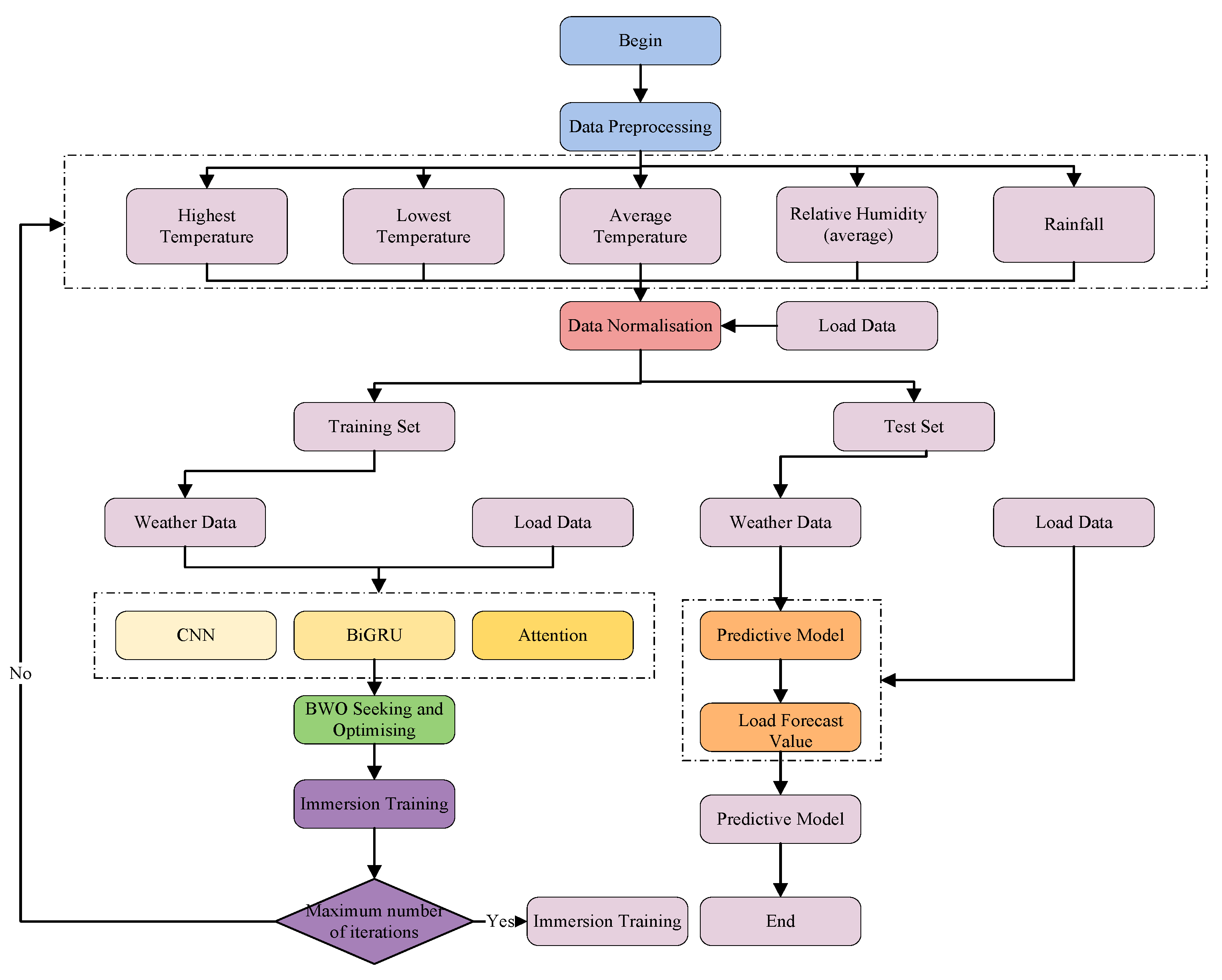
The model constructed in this paper includes multiple optimization steps, the detailed process of which is shown in Figure 3. First, the dataset is preprocessed. Then, meteorological data and historical load data are input, and the dataset is divided into a training set and a test set. The training set is used to train the model, and the test set is used to evaluate model performance. The training set data is then processed using the CNN-BiGRU-Attention model to learn the relationship between meteorological characteristic variables and predicted values. Subsequently, the whale optimization algorithm is used to determine the optimal parameter combination and apply it to the load forecasting model. During this process, the model generates power output forecasts based on the input meteorological data, and finally completes the forecast evaluation.

4. CNN-BiGRU-Attention Based on Whale Optimization

4.1. Convolutional Neural Network(CNN)

To fully explore the interrelationships between electricity loads across different time periods, a CNN module is introduced. This enables automated feature extraction through the use of multiple convolutional kernels with consistent weights, thereby enhancing the quality of data features [21]. The CNN model excels at processing electricity load feature extraction and fusion under the influence of weather characteristics. The CNN layer primarily comprises convolutional layers, pooling layers, and fully connected layers. The convolutional layer consists of a set of small learning convolutional kernels, performing layer-by-layer convolution through trainable kernels and adjustable biases [22]. Input values are mapped to output values within a specific range via the sigmoid activation function, generating feature maps that progressively extract low-level features into high-level features while increasing depth [23]. Each convolution represents the interaction between the input and filter weights [24]. To reduce dimensionality, the pooling layer aggregates statistics from features at different locations through max pooling and average pooling. Finally, the fully connected layer transforms the features into a one-dimensional structure, extracting the feature vector. The CNN architecture is illustrated in Figure 4.

4.2. Bidirectional Gated Recirculation Unit(BiGRU)

To better learn the periodic feature vectors extracted by the CNN layer, this paper employs a GRU model to construct an effective time series prediction model. Figure 5 illustrates the schematic diagram of the GRU. This model is a variant of RNN [25], where GRU integrates the forget gate and output gate of LSTM into the update gate, simplifying the structure of the gating unit, reducing parameter size, and improving computational efficiency [26]. Both GRU and LSTM can overcome the problem of long-term memory loss to some extent, but the GRU structure is a more streamlined design that only includes reset gates (r) and update gates (z), mixing neuron states and hidden states, effectively avoiding the problems of gradient vanishing and exploding [27].

At time step t, let $x_t$, $y_t$ and $h_t$ denote the input, output and hidden layer vectors respectively. The reset gate $r_t$ and update gate are calculated as follows.

$$t_t=\sigma (W_{xr}{x}_t+W_{hr}{h}_{t-1}+b_r)$$

(2)

Here, $\sigma$(.) denotes the activation function, while $W_{xr}$, $W_{hr}$, $W_{xz}$, $W_{hz}$ and $b_r$, $b_z$ represent the sets of weight matrices and bias vectors, respectively. The reset gate $r_t$ determines which information is discarded at the previous time step, whereas the update gate $z_t$ selects which information is passed to the next time step [28]. At time step t, the update formula for the hidden layer vector $h_{xt}$ is:

$${\tilde{h}}_t=tanh(W_{xh}{x}_t+W_{hh}(r_t⨀h_{t-1})+b_r)$$

(3)

$$h_t=(1-z_t)h_{t-1}+z_t\tilde{h}$$

(4)

Here, $\tilde{h}$ denotes the candidate hidden state, tanh (.) represents the hyperbolic tangent activation function, the symbol ⨀ denotes the Hadamard product, $W_{xh}$ and $W_{hh}$ are two weight matrices, $b_r$ is the bias vector, and the final computation result is output as:

$$y_t=\sigma (W_y{h}_t+b_y)$$

(5)

Here, $W_y$ and $b_y$ denote the weight matrix and bias vector of the output layer, respectively. The symbol $\sigma$ denotes scalar multiplication of matrices, tanh represents the Sigmoid activation function, $\mathit{I}-$ denotes the hyperbolic tangent activation function, and indicates that the data propagating forward along this link is $\mathit{I}-z_t$.

Electricity load sequences exhibit characteristics of imbalance, non-linearity, and dynamic behavior. During load forecasting, handling complex time series is crucial [29]. The BiGRU model incorporates GRU network layers with both forward and backward propagation directions. Each time step encompasses the entire input sequence’s information, with its output jointly determined by the states of the forward and backward hidden layers. BiGRU simultaneously considers past and future inputs; this bidirectional information flow enables more effective and comprehensive extraction of input sample features [30,31]. Figure 6 illustrates the BiGRU structure. It enhances GRU capabilities by processing information through its hidden layers in both forward and backward directions.

The output of BiGRU is computed in a step using the following formula:

$$h_t=B_i(H_{C,t-1},H_{C,t}),t\in [1,i]$$

(6)

where, $B_i$ denotes the bidirectional fusion function of BiGRU, $H_{C,t-1}$ is the hidden state of the forward GRU at time step $t-1$, $H_{C,t}$ is the hidden state of the backward GRU at time step t, and i represents the total number of time steps.

4.3. Attention Mechanism(Attention)

During the extraction of load feature information, an excessive emphasis on unimportant features hinders the acquisition of crucial data. The Attention module, by simulating the human brain’s attention allocation mechanism, ingeniously and rationally modulates the intensity of focus on information. It disregards unimportant details, thereby enhancing the efficiency of extracting essential information and reducing the interference of less relevant features on the extraction of key data [32,33]. As illustrated in Figure 7, $x_t$ denotes the input to the BiGRU model, $h_t$ represents the hidden layer output obtained by BiGRU, ${\alpha }_t$ signifies the attention probability distribution output by the attention mechanism to the BiGRU hidden layer, and Y denotes the output optimized by BiGRU through the attention mechanism. The processed output vector $h_t$ from the BiGRU activation layer serves as the input to the attention layer. The relevant weight coefficients for the attention mechanism can be calculated using Equations (7)–(9):

$$e_t=utanh(w{h}_t+b)$$

(7)

$${\alpha }_t={\displaystyle \frac{exp\left(e_t\right)}{{\sum }_{j=1}^t{e}_j}}$$

(8)

$$s_t=\sum _{t=1}^i{\alpha }_t{h}_t$$

(9)

Here, $e_t$ denotes the value of the attention probability distribution determined by the output vector $h_t$ from the GRU network layer at time step t. u and w the weight coefficients, b is the bias coefficient, and $s_t$ denotes the output of the attention layer at time step t. First, the hidden state $h_t$ passing through the BiGRU layer undergoes a nonlinear transformation using the activation function tanh(.), yielding a state $e_t$. Subsequently, the new state is weighted to compute the attention weights [34]. The hidden state $h_t$ is then weighted according to these attention weights, resulting in a new feature vector $s_t$.

4.4. Beluga Whale Optimization(BWO)

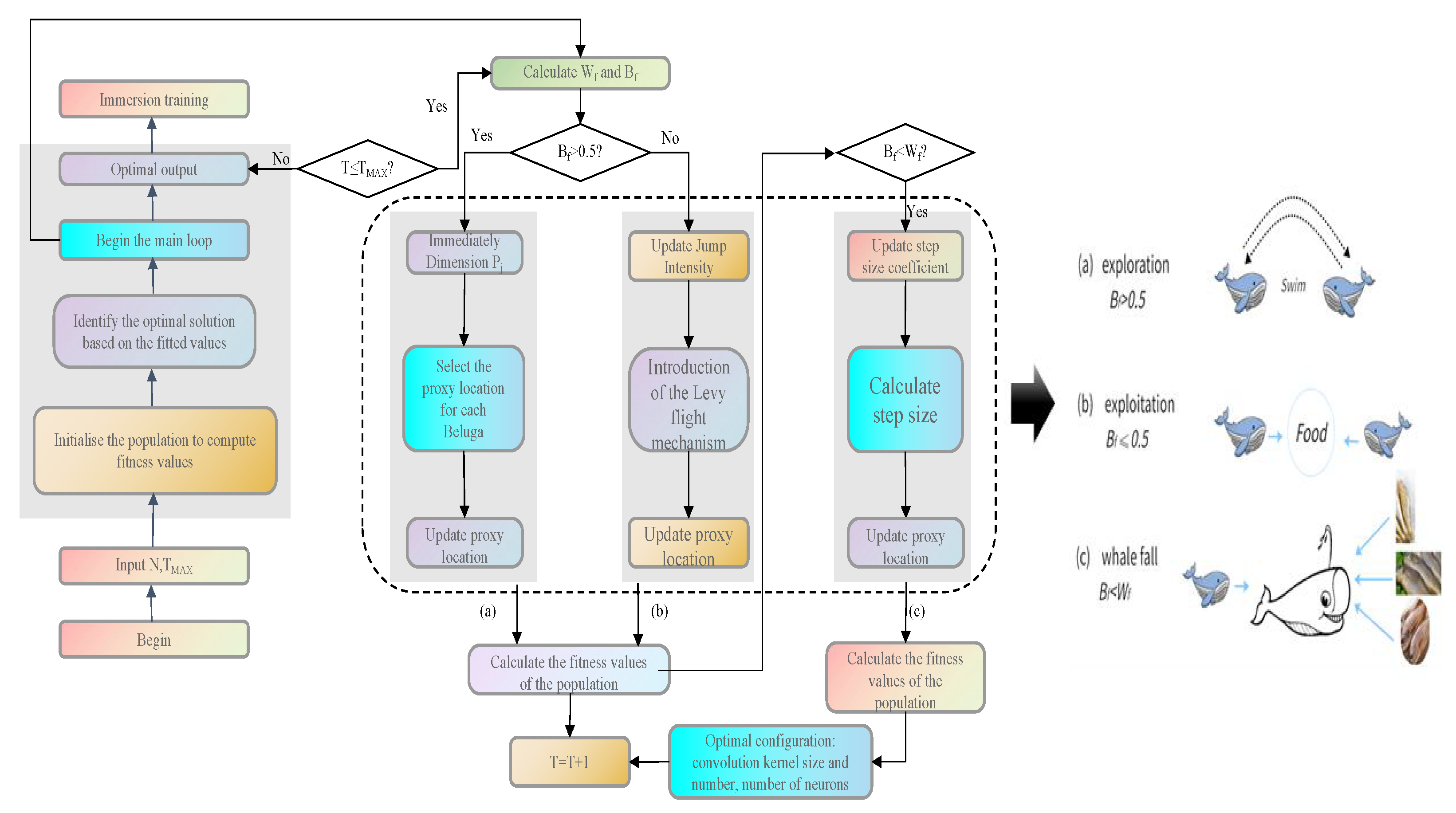
Hybrid models are determined by numerous hyperparameters, such as network depth and learning rate. Finding an optimal combination of hyperparameters is crucial for reducing model complexity and improving algorithm efficiency. This paper introduces the Beluga Whale Optimization Algorithm (BWO) to address the parameter optimization problem in the aforementioned power load forecasting model [19,35]. Inspired by beluga whale behavior, the algorithm consists of three stages: exploration, exploitation, and whale fall. During the exploitation phase, a Levy flight mechanism is introduced to enhance global convergence. The three stages are illustrated in Figure 8.

a. Exploration Phase

First, initialise the algorithm and define the fitness function. Subsequently, enter the exploration phase, updating the proxy positions of a pair of white whales via the following formula.

$$\begin{array}{cc}\hfill & X_{i,j}^{t+1}=X_{i,p_j}^t+(X_{r,p_1}^t-X_{i,p_j}^t)(1+r_1)sin\left(2\pi r_2\right),j=even\hfill \\ \hfill & X_{i,j}^{t+1}=X_{i,p_j}^t+(X_{r,p_1}^t-X_{i,p_j}^t)(1+r_1)cos\left(2\pi r_2\right),j=odd\hfill \end{array}$$

(10)

where T denotes the current iteration, $X_{i,j}^t$ represents the new position of the i beluga in the i dimension, $p_j$ is a random number selected from d dimensions, $X_{i,p_j}^t$ is the position of the i beluga in the $p_j$ dimension, $X_{i,p_j}^t$ and $X_{r,p_j}^t$ denote the current positions of the i and r belugas, respectively, $r_1$ and $r_2$ are random numbers between 0 and 1 to enhance the random operator during the exploration phase. $sin\left(2\pi r_2\right)$ and $cos\left(2\pi r_2\right)$ denote the fin orientations of two mirrored white whales relative to the water surface. Transitioning from the exploration phase to the exploitation phase involves a crucial function—the Balance Factor ($B_f$), whose mathematical model is:

$$B_f=B_0(1-{\displaystyle \frac{t}{2T}})$$

(11)

where t denotes the current iteration, T represents the maximum number of iterations, and $B_0$ fluctuates randomly between (0,1) at each iteration. The exploration phase occurs when the balance factor $B_f>0.5$, whilst the exploitation phase commences when $B_f\le 0.5$. As iteration T increases, the fluctuation range of $B_f$ diminishes from (0,1) to (0, 0.5), indicating a significant shift in the probability distribution between exploration and exploitation phases. The probability of exploitation increases progressively with rising iteration T.

b. Development Phase

This phase is constructed through the hunting behaviour of beluga whales, which capture prey by sharing locations with one another to find the optimal position solution. The Levy mechanism is introduced in this phase to enhance convergence, with its mathematical model as follows:

$$X_i^{t+1}=r_3{X}_{best}^t-r_4{X}_i^t+C_1·L_F·(X_r^t-X_i^t)$$

(12)

where T denotes the current iteration count, $X_i^t$ and $X_r^t$ represent the current positions of the i whale and a randomly selected whale, respectively, $X_i^{t+1}$ denotes the new position of the i whale, $X_{best}^t$ denotes the optimal position among the whales, $r_3$ and $r_4$ denote random numbers within the range (0,1), and $C_1=2r_4(1-T/T_{max})$ is employed to measure the random jump intensity of the Levy flight. $L_F$ denotes the Levy flight function, calculated as follows:

$$L_F=0.05\times {\displaystyle \frac{\mu \times \sigma }{{\left|v\right|}^{1/\beta }}}$$

(13)

$$\sigma ={\left({\displaystyle \frac{\Gamma (1+\beta )\times sin(\pi \beta /2)}{\Gamma ((1+\beta )/2)\times \beta \times 2^{(\beta -1)/2}}}\right)}^{1/\beta }$$

(14)

where $\mu$ and $\sigma$ are normally distributed random numbers, and $\beta$ is the default constant, set to 1.5.

c. Whale Fall Phase

During migration and foraging, a small proportion of beluga whales succumb to attacks by marine predators and sink to the deep sea. This phase simulates such population fluctuations to maintain diversity in the algorithm’s solution space. Unlike PSO, which converges as particles cluster, the Whale Fall ensures that a portion of the population is constantly “reset” to new areas of the search space. This diversity maintenance is mathematically proven to reduce the probability of getting trapped in local optima. The minor fluctuations in beluga populations can be simulated by updating their positions within the model through steps that account for their location and changes in diving depth. This mathematical model is expressed as:

$$X_i^{t+1}=r_5{X}_i^t-r_6{X}_r^t+r_7{X}_{step}$$

(15)

where $r_5$, $r_6$ and $r_7$ are random numbers between (0,1), and $X_{step}$ is the whale fall step size, determined as:

$$X_{step}=(u_b-l_b)exp(-C_2{\displaystyle \frac{t}{T}})$$

(16)

where $C_2$ is the step size factor related to whale fall probability and population size, $C_2=2W_{f\times n}$, with $u_b$ and $l_b$ representing the upper and lower bounds of the variable, respectively. It can be observed that the step size is influenced by the design variables, iteration count, and the boundary of the maximum iteration number. Within this model, the whale descent probability $W_f$ is computed as a linear function:

$$W_f=0.1-0.05t/T$$

(17)

The whale fall probability decreases from 0.1 at the initial iteration to 0.05 at the final iteration, indicating that the whale faces reduced danger as it approaches food sources during the optimization process.

5. Experimental Results

5.1. Evaluation Indicators

To quantify model performance, this paper employs the MAE, RMSE, MAPE, and $R^2$ as evaluation metrics. These metrics effectively elucidate the deviation between predicted and actual values, thereby enabling accurate model assessment.

• MAE (Mean Absolute Error): measures average magnitude of error in MW.
• RMSE (Root Mean Squared Error): By squaring errors, RMSE penalizes large deviations heavily. In grid security, a large prediction error (e.g., missed peak) is far more dangerous than many small errors. Thus, RMSE is the primary metric for operational reliability.
• MAPE (Mean Absolute Percentage Error): provides a percentage-based error measure, critical for economic assessment and electricity market bidding.
• $R^2$ (Coefficient of Determination): Measures how well the model replicates the variance and shape of the load curve.

The calculation formulae for each evaluation metric are as follows.

$$MAPE={\displaystyle \frac{1}{n}}\sum _{i=1}^n\left|{\displaystyle \frac{y_i-{\widehat{y}}_i}{y_i}}\right|$$

(18)

$$RMSE=\sqrt{{\displaystyle \frac{1}{n}}\sum _{i=1}^n{(y_i-{\widehat{y}}_i)}^2}$$

(19)

$$MAE={\displaystyle \frac{1}{n}}\sum _{i=1}^n|y_i-{\widehat{y}}_i|$$

(20)

$$R^2=1-{\displaystyle \frac{{\sum }_{i=1}^n{(y_i-{\widehat{y}}_i)}^2}{{\sum }_{i=1}^n{(y_i-{\overline{y}}_i)}^2}}$$

(21)

where $y_i$ denotes the actual value, ${\overline{y}}_i$ represents the mean of the actual values, ${\widehat{y}}_i$ signifies the predicted value, and n denotes the number of data points.

5.2. Experimental Setup

In the experiment, to achieve optimal predictive outcomes for each model, the control variable method was employed to repeatedly adjust model parameters, thereby optimizing training results. The parameter adjustment process is illustrated below using Model 5 as an example. First, both layers of the BiGRU were fixed at 20 neurones, while the number of CNN layers was adjusted. When the CNN architecture comprised two layers, the Mean Squared Error (MSE) was relatively low. Subsequently, the CNN layers were fixed to determine the optimal number of BiGRU hidden units. The lowest prediction error and highest accuracy were achieved with 20 hidden units. Thereafter, with both CNN and BiGRU layers fixed, the learning rate was adjusted. An MSE of 0.001 demonstrated a significant reduction compared to a learning rate of 0.01. Other parameters were also determined through iterative adjustment and optimization of control variables. Two convolutional layers were employed, each using the same number and size of convolutional kernels, with the sigmoid activation function applied. Pooling layers reduced the feature dimensions by half through multi-dimensional pooling, yielding a final tensor of shape $batc{h}_{s}ize$, filters/2. Subsequently, an attention layer was utilized to weight the transformed features, producing a weighted tensor. Following multiple parameter adjustments, optimal prediction performance was achieved under the following conditions: an initial learning rate of 0.001, 100 iterations, 20 hidden nodes in the BiGRU, a batch size of 16, a convolution kernel size of 3, 24 convolutions, 10 fully connected layer neurones, and a time step of 10. Other models were adjusted using similar methods. Specific parameter values are detailed in

Table 1. Model parameter setting.

Single Model			Mixed Model
Model 1	Model 2	Model 3	Model 4	Model 5	Model 6
$Max\_iter=14$ $Hidden\_layer=100$ $Warm\_start=True$ $Random\_state=4$ $Verbose=True$ $Time\_steps=10$	$Num\_epochs=20$ $Batch\_size=16$ $Lr=0.001$ $Hidden1=10$ $Hidden2=10$ $Fc=10$ $Time\_steps=10$	$Num\_epochs=20$ $Batch\_size=16$ $Lr=0.001$ $Hidden1=10$ $Hidden2=10$ $Fc=20$ $Time\_steps=10$	$Num\_epochs=100$ $Batch\_size=16$ $Lr=0.01$ $Hidden1=10$ $Hidden2=10$ $Fc=10$ $Time\_steps=10$	$Num\_epochs=100$ $Batch\_size=16$ $Lr=0.001$ $Filters=64$ $Filter\_size=3$ $Hidden1=20$ $Hidden2=20$ $Fc=10$ $Time\_steps=1$	$Num\_epochs=100$ $Batch\_size=16$ $Lr=0.001$ $Filters=64$ $Filter\_size=3$ $Hidden1=20$ $Hidden2=20$ $Fc=20$ $Time\_steps=10$ $Dim=4$ $UP=[30,40,100,32]$ $LP=[10,10,50,8]$ $Max\_iter=20$ $N=4$

.

Furthermore, to validate the predictive performance of the proposed model, relevant experimental settings were implemented. The model was first blended layer-by-layer to yield three conventional single models and three layer-by-layer blended models, with experimental results from all six models subsequently compared. The workflow for each model is illustrated in Figure 9.

5.3. Loss Function

In the experiment, the mean square error function (MSE) was used as the loss function to measure the prediction error of the model. The calculation formula is shown in Equation (22).

$$Loss={\displaystyle \frac{1}{n}}\sum _{i=1}^n{(y_i-\overline{y_i})}^2$$

(22)

The loss function is used to measure the difference between the output results of the model and the true labels. In deep learning, the backpropagation algorithm is used to update the parameters of the model to achieve optimal output of the loss function. To further improve the optimization effect, Adam was chosen as the optimiser. Figure 10 shows the loss curves of GRU, BiGRU, BiGRU-Attention, and CNN- BiGRU-Attention.

The loss curves of the six models demonstrate that as the number of iterations increases, both training and testing errors gradually decrease, ultimately converging towards a smaller value. Model 1 converged to approximately 0.1, exhibiting stable convergence albeit at a relatively slow pace. The training and testing errors for the other five models ultimately stabilized near zero. Analysis of training speed and stability revealed that while Models 2 and 3 eventually reached a stable state, the gap between the two lines in their loss curves remained relatively large. Model 4 exhibited rapid oscillations to a low value during the initial phase, indicating unstable training performance. Model 5 displayed a relatively smooth loss curve, suggesting superior model effectiveness. For Model 6, the curve exhibited substantial fluctuations during the initial 40 iterations before gradually levelling off and converging to a low value, thereby validating the model’s training efficacy. In summary, these analyses further corroborate the models’ validity and the effectiveness of the refinement strategy, while also confirming the accuracy of the assumptions and inferences made during model design.

5.4. Model Comparison Analysis

The experimental model 6 (BWO-CNN-BiGRU-Attention) was validated against several other commonly used single and combined models (BP, GRU, BiGRU, BiGRU-Attention, CNN-BiGRU-Attention, BWO-CNN-BiGRU-Attention). The dataset was partitioned into training and test sets, with the final two days of data reserved for testing and the remainder used for training.

To quantify the contribution of each component, an ablation study was conducted as detailed in

Table 2. Ablation Study Results.

Model	Architecture	MAPE	RMSE	MAE	${\mathit{R}}^2$	Improvement Logic
Model 1	BP	5.821	345.67	278.45	0.8277	Baseline
Model 2	GRU	3.456	210.34	165.23	0.9302	+ Temporal memory (captures sequence).
Model 3	BiGRU	2.631	158.92	125.67	0.9436	+ Bidirectionality (captures future context).
Model 4	BiGRU-Attn	2.158	132.45	103.12	0.9521	+ Attention (weights critical moments).
Model 5	CNN-BiGRU-Attn	1.783	105.78	80.56	0.9619	+ Spatial features (CNN cleans input).
Model 6	BWO-Optimized	1.585	92.46	63.5	0.9758	+ Global Optimization (avoids local optima).

. The limitations of the baseline BP model (Model 1) were evident, with an RMSE of 345.67. The introduction of temporal sequence modeling in GRU (Model 2) and BiGRU (Model 3) significantly improved performance, reducing RMSE to 210.34 and 158.92, respectively, while increasing $R^2$ to over 0.94. The subsequent integration of the Attention mechanism (Model 4) and CNN spatial feature extraction (Model 5) further refined predictive accuracy, yielding an MAPE of 1.783%. Ultimately, the proposed BWO-optimized framework (Model 6) achieved the best overall performance (MAPE: 1.585%, RMSE: 82.46, $R^2$: 0.9758). Notably, compared to Model 5, the BWO optimization reduced the RMSE by approximately 12.6%, validating its effectiveness in avoiding local optima and enhancing model robustness.

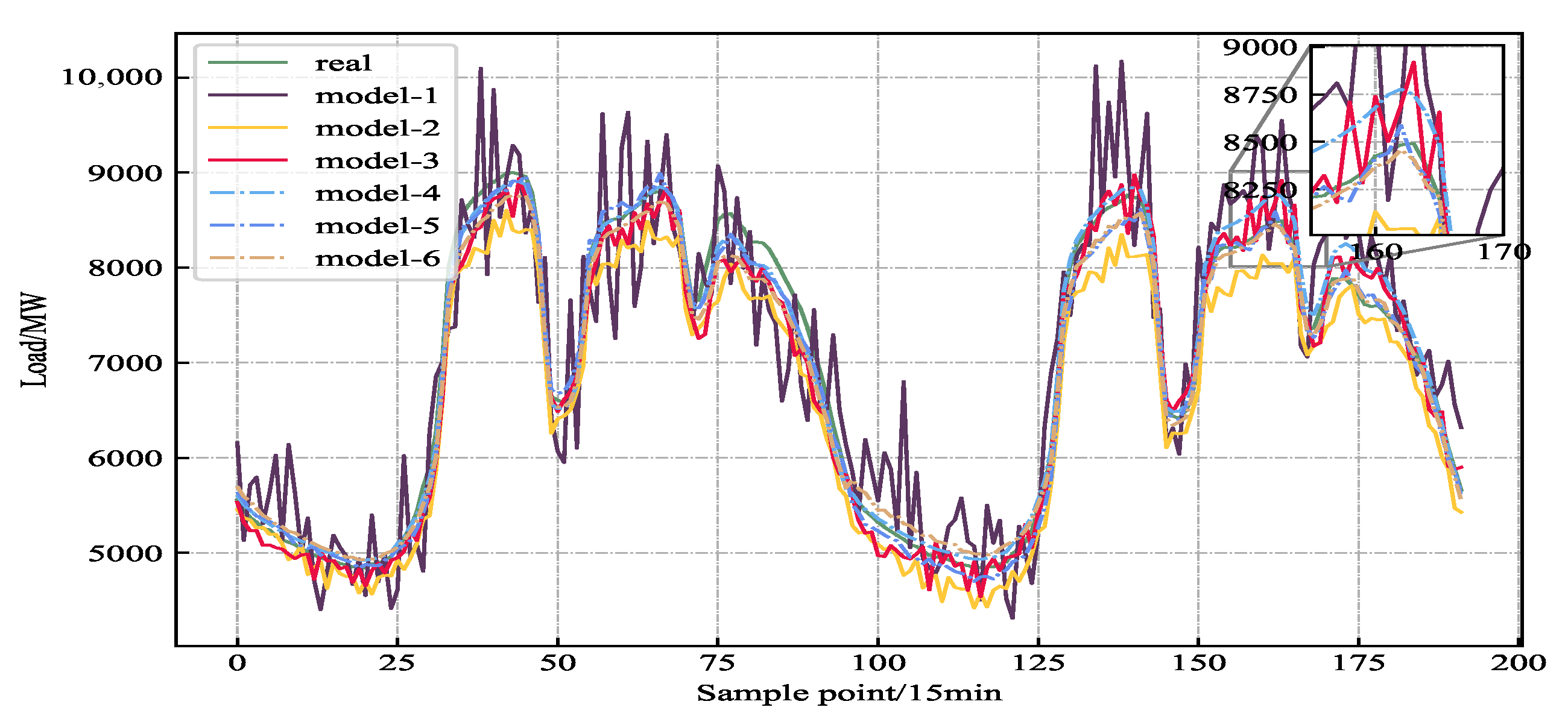
Following multiple tests, predictions were generated for each model by partitioning the dataset into training and test sets. The final two days’ data, specifically 9 January 2020 and 10 January 2020, constituted the test set, with the remaining data serving as the training set. The test set predictions are presented in Figure 11a–f, encompassing 192 data points. The figures reveal that the predictive performance of each model exhibits certain discrepancies at both peak and trough values. Nevertheless, our proposed model demonstrates superior fitting capabilities compared to other baseline models, particularly in capturing both peak and trough values.

By examining Figure 12, it is evident that the predictions generated by the CNN-BiGRU-Attention model, optimized using the BWO algorithm for parameter tuning, align more closely with actual conditions. The superior line-fitting performance between the two further validates the superiority of the proposed hybrid model. For models with a substantial number of parameters, the BWO algorithm achieves effective parameter tuning.

To comprehensively demonstrate the models’ performance, polar plots of the training errors for all six models were generated. Models 1 through 6 are depicted in Figure 13, respectively. Upon observing the curves, it was noted that the final loss values for each model stabilized near specific points, indicating that the models gradually converged to a stable state during the training process. In particular, a highly concentrated error distribution near the origin was exhibited by Model 6, whereas scattered deviations were displayed by the baseline models. The statistical conclusion of higher stability is supported by these visualization results.

5.5. Convergence Effect of the Optimized White Whale Model

As shown in Figure 14, the fitness iteration curve based on the BWO optimization model was plotted to assess the algorithm’s convergence. The curve was constructed using the optimal fitness values obtained at each iteration of the BWO optimization process.

The parameters of the model were optimized using the Beluga optimization algorithm, and the optimal parameters found were: $hidden1=10, hidden2=10, filters=50, batch\_size=8$. During each iteration, the parameter values of the current iteration are passed in, the model is trained, and the prediction results on the test data are obtained. Then, the RMSE between the prediction results and the true labels is calculated as the fitness value for that iteration. Finally, the fitness values of all iterations are plotted as a fitness curve.

By observing the iteration curve, it can be found that as the number of iterations increases, the fitness value gradually decreases and stabilizes at around 0.235, showing a stable convergence trend. This indicates that using BWO to find the optimal combination of hybrid model parameters effectively reduces the randomness of empirically set parameters and improves the optimization performance of the model.

6. Conclusions and Future Works

In summary, the CNN-BiGRU-Attention model based on Beluga Whale Optimization proposed in this paper demonstrates high accuracy in short-term power load forecasting. By combining modules such as CNN, BiGRU, and Attention, it can better utilize the feature information and time series data of historical load sequences, thereby improving the prediction effect. In addition, optimizing the model parameters through the BWO algorithm can further enhance the model’s fitting ability. The model can be applied to practical scenarios such as power grid day-ahead scheduling, renewable energy integration optimization, and power cost control, providing technical support for the stable operation of power systems.

While the current experiment focuses on a specific short-term testing window to simulate immediate dispatching needs, we acknowledge that the relatively short test duration limits the assessment of long-term robustness. Future research can focus on three directions: (1) simplify the model structure using lightweight convolutional kernels (e.g., depthwise separable convolution) and pruning techniques to improve inference efficiency; (2) expand the dataset to encompass multiple years and validate the model on larger test sets, including extreme weather and holiday load data, and introduce transfer learning to enhance the model’s generalization ability under special scenarios; and (3) integrate multi-source data (e.g., economic indicators, user behavior data) to further improve prediction accuracy.

References

1. Dong, Q.; Huang, R.; Cui, C.; Towey, D.; Zhou, L.; Tian, J.; Wang, J. Short-Term Electricity-Load Forecasting by deep learning: A comprehensive survey. Eng. Appl. Artif. Intell. 2025, 154, 110980. [Google Scholar] [CrossRef]
2. Al-Bossly, A. Metaheuristic Optimization with Deep Learning Enabled Smart Grid Stability Prediction. Comput. Mater. Contin. 2023, 75, 6395. [Google Scholar] [CrossRef]
3. Aguilar Madrid, E.; Antonio, N. Short-term electricity load forecasting with machine learning. Information 2021, 12, 50. [Google Scholar] [CrossRef]
4. Shuang, R.; Kai, Y.; Jicai, S.; Jiming, Q.; Xiangyu, W.; Yonggen, C. Short-term Power Load Forecasting Based on CNN-BiGRU-Attention. J. Electr. Eng. 2024, 19, 344–350. [Google Scholar]
5. Liu, X.; Song, J.; Tao, H.; Wang, P.; Mo, H.; Du, W. Quarter-Hourly Power Load Forecasting Based on a Hybrid CNN-BiLSTM-Attention Model with CEEMDAN, K-Means, and VMD. Energies 2025, 18, 2675. [Google Scholar] [CrossRef]
6. Mumtahina, U.; Alahakoon, S.; Wolfs, P. Hyperparameter tuning of load-forecasting models using metaheuristic optimization algorithms—a systematic review. Mathematics 2024, 12, 3353. [Google Scholar] [CrossRef]
7. Yang, J.; Xing, C. Data source selection based on an improved greedy genetic algorithm. Symmetry 2019, 11, 273. [Google Scholar] [CrossRef]
8. Chen, P.; Liu, P.; Lan, L.; Guo, M.; Guo, H. Enhancing Accuracy in Wind and Photovoltaic Power Forecasting Through Neutral Network and Beluga Whale Optimization Algorithm. Int. J. Multiphys. 2024, 18, 85. [Google Scholar]
9. Youssef, H.; Kamel, S.; Hassan, M.H.; Mohamed, E.M.; Belbachir, N. Exploring LBWO and BWO algorithms for demand side optimization and cost efficiency: Innovative approaches to smart home energy management. IEEE Access 2024, 12, 28831–28852. [Google Scholar] [CrossRef]
10. Liu, X.; Lin, Z.; Feng, Z. Short-term offshore wind speed forecast by seasonal ARIMA-A comparison against GRU and LSTM. Energy 2021, 227, 120492. [Google Scholar] [CrossRef]
11. Subbiah, S.S.; Chinnappan, J. Deep learning based short term load forecasting with hybrid feature selection. Electr. Power Syst. Res. 2022, 210, 108065. [Google Scholar] [CrossRef]
12. Wazirali, R.; Yaghoubi, E.; Abujazar, M.S.S.; Ahmad, R.; Vakili, A.H. State-of-the-art review on energy and load forecasting in microgrids using artificial neural networks, machine learning, and deep learning techniques. Electr. Power Syst. Res. 2023, 225, 109792. [Google Scholar] [CrossRef]
13. Wang, H.; Zhang, N.; Du, E.; Yan, J.; Han, S.; Liu, Y. A comprehensive review for wind, solar, and electrical load forecasting methods. Glob. Energy Interconnect. 2022, 5, 9–30. [Google Scholar] [CrossRef]
14. Niu, D.; Yu, M.; Sun, L.; Gao, T.; Wang, K. Short-term multi-energy load forecasting for integrated energy systems based on CNN-BiGRU optimized by attention mechanism. Appl. Energy 2022, 313, 118801. [Google Scholar] [CrossRef]
15. Fargalla, M.A.M.; Yan, W.; Deng, J.; Wu, T.; Kiyingi, W.; Li, G.; Zhang, W. TimeNet: Time2Vec attention-based CNN-BiGRU neural network for predicting production in shale and sandstone gas reservoirs. Energy 2024, 290, 130184. [Google Scholar] [CrossRef]
16. Lu, P.; Ye, L.; Zhao, Y.; Dai, B.; Pei, M.; Tang, Y. Review of meta-heuristic algorithms for wind power prediction: Methodologies, applications and challenges. Appl. Energy 2021, 301, 117446. [Google Scholar] [CrossRef]
17. Zhong, C.; Li, G.; Meng, Z. Beluga whale optimization: A novel nature-inspired metaheuristic algorithm. Knowl.-Based Syst. 2022, 251, 109215. [Google Scholar] [CrossRef]
18. Asiri, M.M.; Aldehim, G.; Alotaibi, F.A.; Alnfiai, M.M.; Assiri, M.; Mahmud, A. Short-term load forecasting in smart grids using hybrid deep learning. IEEE Access 2024, 12, 23504–23513. [Google Scholar] [CrossRef]
19. Li, Z.; Gao, J.; Guo, J.; Xie, Y.; Yang, X.; Li, M.J. Optimal loading distribution of chillers based on an improved beluga whale optimization for reducing energy consumption. Energy Build. 2024, 307, 113942. [Google Scholar] [CrossRef]
20. Niu, D.; Wang, K.; Sun, L.; Wu, J.; Xu, X. Short-term photovoltaic power generation forecasting based on random forest feature selection and CEEMD: A case study. Appl. Soft Comput. 2020, 93, 106389. [Google Scholar] [CrossRef]
21. Hong, Y.Y.; Chan, Y.H. Short-term electric load forecasting using particle swarm optimization-based convolutional neural network. Eng. Appl. Artif. Intell. 2023, 126, 106773. [Google Scholar] [CrossRef]
22. Huang, Q.; Li, J.; Zhu, M. An improved convolutional neural network with load range discretization for probabilistic load forecasting. Energy 2020, 203, 117902. [Google Scholar] [CrossRef]
23. Aurangzeb, K.; Alhussein, M.; Javaid, K.; Haider, S.I. A pyramid-CNN based deep learning model for power load forecasting of similar-profile energy customers based on clustering. IEEE Access 2021, 9, 14992–15003. [Google Scholar] [CrossRef]
24. Zhao, B.; Wang, Z.; Ji, W.; Gao, X.; Li, X. A short-term power load forecasting method based on attention mechanism of CNN-GRU. Power Syst. Technol. 2019, 43, 4370–4376. [Google Scholar]
25. Wang, K.; Liu, C.; Duan, Q. Piggery ammonia concentration prediction method based on CNN-GRU. J. Phys. Conf. Ser. 2020, 1624, 042055. [Google Scholar] [CrossRef]
26. Wahab, A.; Tahir, M.A.; Iqbal, N.; Ul-Hasan, A.; Shafait, F.; Kazmi, S.M.R. A novel technique for short-term load forecasting using sequential models and feature engineering. IEEE Access 2021, 9, 96221–96232. [Google Scholar] [CrossRef]
27. Sun, F.; Huo, Y.; Fu, L.; Liu, H.; Wang, X.; Ma, Y. Load-forecasting method for IES based on LSTM and dynamic similar days with multi-features. Glob. Energy Interconnect. 2023, 6, 285–296. [Google Scholar] [CrossRef]
28. Aurangzeb, K.; Alhussein, M. Deep learning framework for short term power load forecasting, a case study of individual household energy customer. In Proceedings of the 2019 International Conference on Advances in the Emerging Computing Technologies (AECT), Al Madinah Al Munawwarah, Saudi Arabia, 10 February 2020; pp. 1–5. [Google Scholar]
29. Sabatello, M.; Martschenko, D.O.; Cho, M.K.; Brothers, K.B. Data sharing and community-engaged research. Science 2022, 378, 141–143. [Google Scholar] [CrossRef]
30. Du, L.; Zhang, L.; Wang, X. Spatiotemporal feature learning based hour-ahead load forecasting for energy internet. Electronics 2020, 9, 196. [Google Scholar] [CrossRef]
31. Kisvari, A.; Lin, Z.; Liu, X. Wind power forecasting–A data-driven method along with gated recurrent neural network. Renew. Energy 2021, 163, 1895–1909. [Google Scholar] [CrossRef]
32. Wang, S.; Shi, J.; Yang, W.; Yin, Q. High and low frequency wind power prediction based on Transformer and BiGRU-Attention. Energy 2024, 288, 129753. [Google Scholar] [CrossRef]
33. Gong, P.; Luo, Y.; Fang, Z.M.; Dou, F. Short-term power load forecasting method based on Attention-BiLSTM-LSTM neural network. J. Comput. Appl. 2021, 41, 81–86. [Google Scholar]
34. Zhou, G.; Hu, G.; Zhang, D.; Zhang, Y. A novel algorithm system for wind power prediction based on RANSAC data screening and Seq2Seq-Attention-BiGRU model. Energy 2023, 283, 128986. [Google Scholar] [CrossRef]
35. Horng, S.C.; Lin, S.S. Improved beluga whale optimization for solving the simulation optimization problems with stochastic constraints. Mathematics 2023, 11, 1854. [Google Scholar] [CrossRef]
Figure 1. Overview of the dataset.
Information 17 00006 g001aInformation 17 00006 g001b
Figure 2. Correlation matrix of features.
Information 17 00006 g002
Figure 3. Process of the proposed framework.
Information 17 00006 g003
Figure 4. CNN architecture.
Information 17 00006 g004
Figure 5. GRU structure diagram.
Information 17 00006 g005
Figure 6. BiGRU structure diagram.
Information 17 00006 g006
Figure 7. Attention mechanism.
Information 17 00006 g007
Figure 8. Beluga Whale Optimization Algorithm flow.
Information 17 00006 g008
Figure 9. Model comparison process.
Information 17 00006 g009
Figure 10. Loss curves of the six models.
Information 17 00006 g010
Figure 11. Prediction results of the six models.
Information 17 00006 g011
Figure 12. Prediction results.
Information 17 00006 g012
Figure 13. Polar plots of training errors for the six models.
Information 17 00006 g013
Figure 14. Fitness iteration curve of the proposed model.
Information 17 00006 g014