DIP-UP: Deep Image Prior for Unwrapping Phase

Abstract

Phase images from gradient echo MRI sequences reflect underlying magnetic field inhomogeneities but are inherently wrapped within the range of −π to π, requiring phase unwrapping to recover the true phase. In this study, we present DIP-UP (Deep Image Prior for Unwrapping Phase), a framework designed to refine two pre-trained deep learning models for phase unwrapping: PHUnet3D and PhaseNet3D. We compared the DIP-refined models to their original versions, as well as to the conventional PRELUDE algorithm from FSL, using both simulated and in vivo brain data. Results demonstrate that DIP refinement improves unwrapping accuracy (achieving ~99%) and robustness to noise, surpassing the original networks and offering comparable performance to PRELUDE while being over three times faster. This framework shows strong potential for enhancing downstream MRI phase-based analyses.

1. Introduction

Magnetic Resonance Imaging (MRI) signals from a Gradient Recalled Echo (GRE) sequence contain phase information proportional to the magnetic field and Echo Time [1,2,3]. Typically, the phase image reflects the inhomogeneities of the magnetic field B0 [4,5]. Many quantitative MRI applications utilize the phase value, such as quantitative susceptibility mapping (QSM) [3,6,7]. Due to the MRI acquisition scheme, the phase value is converted from complex data and folded within the range of −π to π [8]. This restricted range results in discontinuous regions between phase-jumped voxels, forming a series of boundaries. Consequently, phase unwrapping is often approached as a classification issue, aiming to categorize the regions outlined by these boundaries. Misclassified wrapping counts can cause an overall shift in the phase value within a particular brain tissue. Such errors propagate to subsequent procedures like background field removal [9,10] and dipole inversion [11,12]. As a result, the distribution of the resulting susceptibility map may be miscalculated. Additionally, the unwrapping process faces challenges from significant noise in the acquisitions.

Numerous conventional algorithms have been developed to address the phase unwrapping problem, with many falling into two main categories: global optimization [13,14,15,16] and path-based region growing. In the global optimization approach, Marvin et al. [17] presented a valid method by calculating the second-dimensional Laplacian of both the raw and unwrapped phase formulations. Another method, called PRELUDE [18], introduced a phase-partitioning scheme and performed unwrapping within two sub-blocks, demonstrating robustness against noisy data. However, PRELUDE had limitations when creating initial regions, as the algorithm failed when the gap between two voxels exceeded 2π. Building upon PRELUDE, Karsa et al. [19] developed an acceleration scheme that reduced the processing time from 20 min to 30 s. Their method, SEGUE, was successfully implemented on 3D human brains. Despite its improved efficiency, SEGUE was sensitive to noise and its accuracy sharply decreased when dealing with low signal-to-noise ratio data. Furthermore, the three global optimization methods were computationally intensive and resource intensive. Alternatively, other approaches addressed the phase unwrapping problem using the path-based region-growing technique, which significantly reduced processing time. Hussein et al. [20] extended this technique from 2D to 3D images. Their method involved a sequential flow of reliable paths aligned by voxel quality. Another path-based algorithm, commonly referred to as the Best-Path (BP) method, simplified the global computation by detecting voxels on discontinuous boundaries. Moreover, 3D-BP proposed a hybrid technique that combined the path-based approach with a noise-immune algorithm [21]. However, both path-based methods showed limited capability in denoising with a low signal-to-noise ratio. Cheng et al. [22] proposed CLOSED3D, which drew upon the region-growing methodology from Best-Path and applied it to 3D QSM data. Although CLOSED3D achieved accuracy and robustness using a 26-neighborhood relationship, it still had drawbacks, such as low coding efficiency and a lack of flexibility in parameter tuning.

Recently, deep learning methods have been investigated and have shown significant improvements over conventional approaches [23,24,25,26]. Utilizing neural networks, well-trained models have been able to reduce processing time by 50% [27,28] while maintaining an accuracy of 90%. Moreover, several deep learning methods have achieved multi-condition inference using single-mode datasets, such as training on ‘clean’ data and testing on acquisitions with noise. In the field of phase unwrapping, deep learning methods have made advancements. PhaseNet [29] was one of the initial networks developed, aiming to classify wrapping counts using cross-entropy loss. This network increased the quantity of training labels through synthetic data and explored post-processing methods to address misclassifications. The improved version, PhaseNet 2.0 [30], modified the post-processing algorithm and incorporated it into the loss function. PhaseNet 2.0 introduced 10 dB noise to the original dataset, enabling generalized inference. Additionally, the unsupervised training network PU-GAN [31] was built on GAN [32], overcoming the limitations of traditional unwrapping methods based on the Itoh condition. However, these models were trained only on optical 2D data, lacking the typical structures present in brain MR images. To address this limitation, Zhou et al. [33] proposed PHU-NET using simulated MR images, demonstrating robustness against 20 dB noise. Furthermore, PHU-NET [33] removed the cross-entropy loss and modified the residue loss from PhaseNet 2.0, simplifying the network structure and reducing training time. Although PHU-NET has shown general capability with multiple MRI datasets, it still faces limitations such as training on 2D data and restricted noise levels. Yang et al. [11] introduced an end-to-end network that directly processes raw phase data into resulting QSM, bypassing post-processing steps like phase unwrapping, background field removal, and dipole inversion. This approach significantly reduces the overall processing time. Another unified network, Unet-QSM [7], was trained using multi-echo phase data. However, both iQSM and Unet-QSM fail to preserve unwrapped phase images, limiting their flexibility in assessing main field homogeneity and related magnetic field properties. Furthermore, Chen et al. established an unsupervised scheme via a phase-encoded unrolling network [34]. Wei et al. extended the spatial unwrapping into the temporal domain [35] and Boroujeni et al. implemented the GAN-based phase-segmentation into the graphic forest fire monitoring [36], which expanded the application of NN applications.

Although pre-trained networks have demonstrated certain capabilities, they often suffer from limitations related to the modality and quality of training data. To address these issues, Deep Image Prior [37] (DIP) has emerged as a novel approach to image restoration tasks without the need for extensive training datasets. DIP leverages the structure of untrained neural networks to reconstruct high-quality images from corrupted or incomplete inputs. Xiong et al. [38] applied DIP to QSM dipole inversion by incorporating untrained neural networks and structural information, effectively overcoming traditional limitations in image denoising. Yang et al. [39] expanded the idea to phase unwrapping, combining the variational framework and a Unet-based ‘blank’ network. Building on prior studies, our work is the first to integrate DIP with pre-trained 3D networks, overcoming the 2D limitations of PhaseNet 2.0 [30] while maintaining computational efficiency. In addition, we introduce physics-guided unsupervised refinement without relying on labeled data.

2. Materials and Methods

2.1. Theory

Phase data from MRI acquisition is proportional to the echo time and main field:

$$\phi =-\gamma ·\Delta B·TE,$$

(1)

where $\phi$ represents the phase value and $\gamma$ stands for the gyromagnetic ratio. $\Delta B$ and $TE$ refer to the field perturbation and echo time, respectively.

The mathematical relationship between the raw phase $\psi$ and the unwrapped true phase $\phi$ could be performed as follows:

$${\phi }_{(x,y,z)}={\psi }_{(x,y,z)}+2\pi ·k_{(x,y,z)},$$

(2)

The subscript ($x, y, z$) denotes the spatial coordinates of a voxel in the brain image and $k$ represents the wrapping counts, which is an integer. The unwrapped phase value is calculated by raw phase adding the wrapping count multiple of $2\pi$.

2.2. Training Data Simulation

Full-size (matrix size 144 × 192 × 128) human brains were obtained from 96 in vivo subjects (1 mm isotropic at 3T) and were generated by processing the multi-echo GRE raw phase data. Institutional ethics board approval was obtained at the University of Calgary and all subjects gave informed written consent. Tissue brain extraction was performed with the BET toolbox [40] and the raw phase was unwrapped with the Best-Path method [20] for each echo. As illustrated in Figure 1, the field-strength normalized map, or the total field map $\delta B$, was used to simulate the unwrapped phase φ by multiplying the $\gamma$, TE, and B₀.

$$\phi =\delta B ·\gamma ·TE·B_0,$$

(3)

To generate the training input (wrapped phase $\psi$), we converted the simulated unwrapped phase φ into the complex region ${\phi }_c$ according to Euler’s formula:

$${\phi }_c=exp (1j·\phi )$$

(4)

The simulated raw phase ψ, which is considered as the first input channel to neural networks, is obtained by extracting the angle of the resulting complex data ${\phi }_c$:

$$\psi =\mathrm{a}\mathrm{n}\mathrm{g}\mathrm{l}\mathrm{e} \left({\phi }_c\right)$$

(5)

Furthermore, Laplacian maps were calculated as the second channel to the neural networks, as the restriction term of wrapping edges. the Laplacian map of each full-brain image (matrix size 144 × 192 × 128) was calculated by convoluting the simulated raw phase with the 27-point stencil kernel (dker, kernel size: 3 × 3 × 3, by default parameter):

$${\nabla }^2\psi =\mathrm{c}\mathrm{o}\mathrm{n}\mathrm{v} (\psi , dker)$$

(6)

Similar to the previous learning-based methods, the wrapping counts k are regarded as a training label (matrix size 144 × 192 × 128) in this proposed network. Based on Equation (2), the wrapping count k is calculated as follows:

$$k_{\left(x,y,z\right)}={\displaystyle \frac{ {\phi }_{\left(x,y,z\right)}-{\psi }_{\left(x,y,z\right)}}{2\pi }}$$

(7)

These full-size images were trained on 28,800 small patches (matrix size: 643) with 300 patches cropped randomly from each full-brain volume. Patches of the raw phase and Laplacian maps were cropped via the same coordinate as Channels 1 and 2, matching the label patches (i.e., wrapping counts) in space.

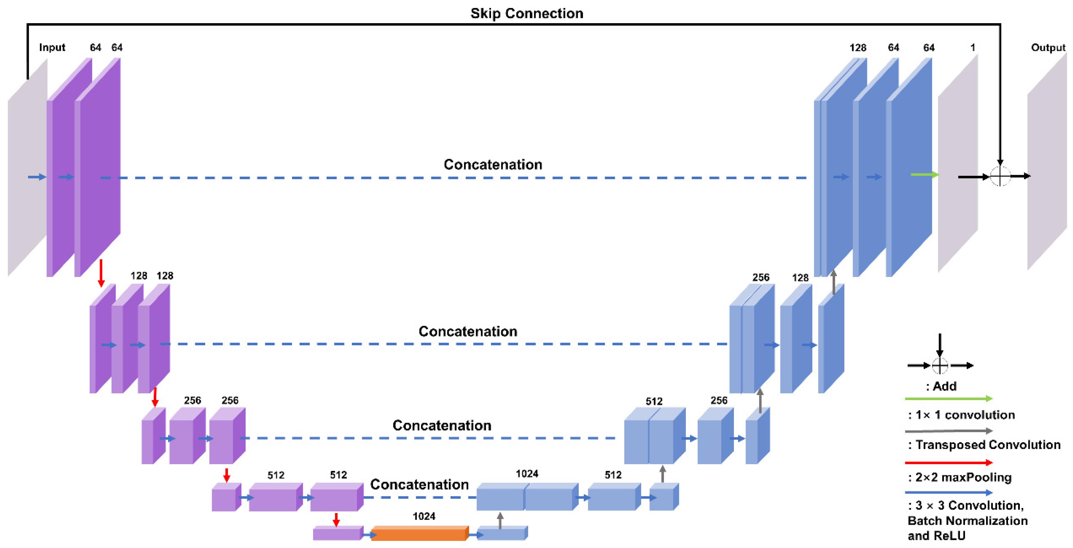
2.3. Network Framework

We used the fundamental U-net as the basic framework of training step, illustrated in Figure 2. The network architecture is structured with two primary functions, encoding and decoding, which are synonymous with the down-sampling and up-sampling paths, respectively. This framework is composed of 18 convolutional blocks. Within each block, there is a convolutional layer with a kernel size of 3 × 3 × 3, followed by batch normalization layers. The Rectified Linear Unit (ReLU) serves as the activation function, and the network utilizes the Root Mean Square propagation (RMSprop) optimizer, with a learning rate set at 10⁻⁴. Moreover, 4 max-pooling layers and 4 transposed convolution layers (kernel size of 2 × 2 × 2) were adopted to compress/recover the image dimension.

In conventional classification methods, cross-entropy (CE) loss is usually implemented. In this study, we designed another two loss functions, including L1-norm loss and L2-norm gradient residual loss. The idea was inspired from two published unwrapping networks: PHU-Net [33] and PhaseNet 2.0 [30].

(a)

Voxel-wised cross-entropy loss function. Cross-entropy loss is used to classify the predicted wrapping counts:

$${Loss}_{CE}=-{\displaystyle \frac{1}{N}}\sum Y(x,y,z)\mathrm{l}\mathrm{o}\mathrm{g}(\tilde{Y}\left(x,y,z\right))$$

(8)

where N refers to the size of the image and Y and $\tilde{Y}$ indicate the ground truth and predicted wrapping counts at the voxel coordination $(x,y,z)$. The SoftMax classifier is connected as the output layer.

(b)

L1-norm loss function: The L1-norm between the predicted and the original unwrapped phase is given by the following:

$${Loss}_{L1}={\displaystyle \frac{1}{N}}\sum |\phi \left(x,y,z\right)-\tilde{\phi }\left(x,y,z\right)|$$

(9)

where $\phi$ and $\tilde{\phi }$ represent for the label and the reconstructed unwrapped phase (calculated from Equation (2)).

(c)

Gradient residue loss function. This is a redesigned version of the PhaseNet 2.0 loss function [30], which was extended to 3D data. In contrast to 2D inference data, 3D brain volumes require more specific and accurate tuning of wrapping boundary detection. As a result, we modified the PhaseNet 2.0 equation by calculating the sum of the squared image gradients across three dimensions. The modification is given by

$${Loss}_{Res}=\sqrt{{\displaystyle \frac{1}{N}}\sum \begin{array}{c}(\left|U_x^2\left(\psi \right)-U_x^2\left(\phi \right)\right|+\\ \left|U_y^2\left(\psi \right)-U_y^2\left(\phi \right)\right|+\\ \left|U_z^2\left(\psi \right)-U_z^2\left(\phi \right)\right|) \end{array}}$$

(10)

where $U_{(x/y/z)}$() refers to the ‘wrapping-boundary masked’ gradient operation of the image via three dimensions. We modified the previous gradient operation and masked the gradient map using a threshold of 1.0π, which erased the border of wrapping while maintaining the brain tissue.

In this study, we implemented combinations of loss functions alongside different input channels in two distinct training modes. The first neural network, inspired by PHUnet [33], was enhanced by upgrading the original 2D training sets to 3D, resulting in PHU-NET3D. Unlike the boundary-pixel identification feature in the original PHUnet, we utilized Laplacian maps to emphasize boundary features between wrapping counts, using raw phase data and corresponding Laplacian maps as dual input channels. Additionally, PHUnet3D improved upon loss function application by exclusively using the cross-entropy (CE) loss function, rather than the L1+Res loss utilized in previous studies [33].

The second network model adopted the multi-loss-function architecture from PhaseNet 2.0 [30], with the total loss defined in Equation (11). Compared to PhaseNet 2.0, we replaced the original residual loss’s L1-norm with an L2-norm. Furthermore, the training set was augmented by switching from 2D to 3D patches while maintaining the original single channel (channel 1) input, which consists of raw phases. This updated approach is referred to as PhaseNet3D.

$${Loss}_{PhaseNet3D}={Loss}_{CE}+{Loss}_{L1}+{Loss}_{Res}$$

(11)

Both networks took around 40 h (45 epochs) in the training using 2 NVIDIA Tesla V100 GPUs (NVIDIA Corporation, Santa Clara, CA, USA) with a minibatch size of 24. The networks were implemented using Pytorch version 3.6.

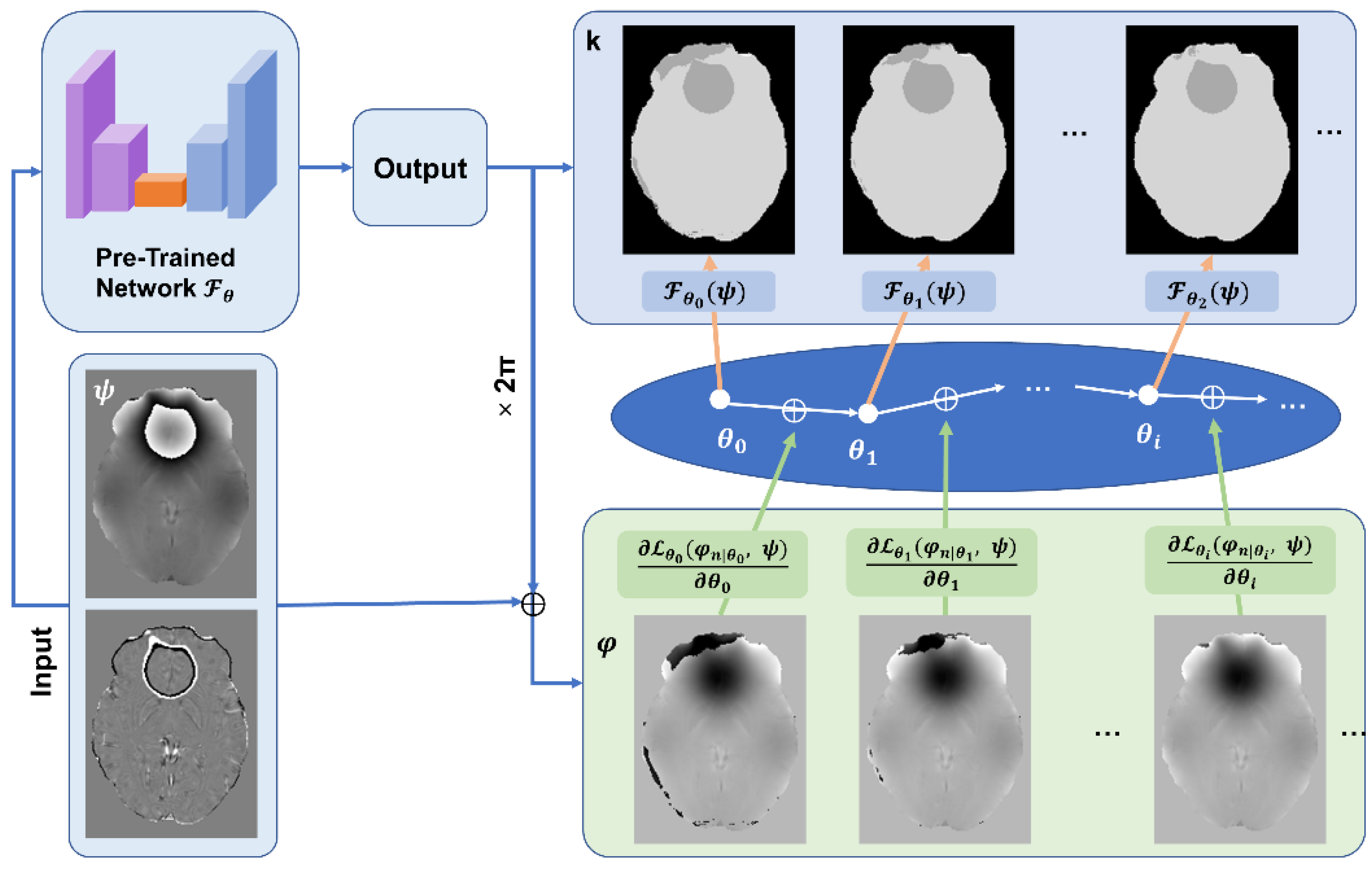
2.4. Deep Image Prior

The DIP method is introduced to improve raw predictions from the pre-trained networks, and the overall scheme is demonstrated in Figure 3. We utilized a mixed-loss function that incorporates both physical model and morphological feature, in order to compensate for the mis-classification regions from the initial prediction from the pre-trained networks.

(1)

The Laplacian loss: This loss function was established based on the physical model [17], such that the Laplacian of the unwrapped phase φ can be calculated from the raw wrapped phase ψ:

$${\nabla }^2\phi =cos\left(\psi \right){\nabla }^{2}sin\left(\psi \right)-sin\left(\psi \right) {\nabla }^{2}cos\left(\psi \right)$$

(12)

where the Laplacian of unwrapped phase could be calculated through Equation (6), given that

$${\nabla }^2\left(\phi \right)=\mathrm{c}\mathrm{o}\mathrm{n}\mathrm{v} (\phi , dker)$$

(13)

Combined the Equations (12) and (13), the Laplacian loss could be used to minimize the difference between the Laplacian of the recon-unwrapped phase and the raw (wrapped) phase. The difference is calculated through the L1-norm.

$$\begin{gathered} {Loss}_{Lap}={\displaystyle \frac{1}{N}}\sum |{\nabla }^2{\phi }_{pre}-(\cos \left({\psi }_{raw}\right){\nabla }^2\mathrm{s}\mathrm{i}\mathrm{n}\left({\psi }_{raw}\right) \\ -\sin \left({\psi }_{raw}\right){\nabla }^2\mathrm{c}\mathrm{o}\mathrm{s}\left({\psi }_{raw}\right)\left)\right| \end{gathered}$$

(14)

where ${\phi }_{pre}$ and ${\psi }_{raw}$ represent the predicted unwrapped phase and raw phase image, respectively. ${\phi }_{pre}$ was calculated via Equation (2).

(2)

Total Variation (TV) loss: To provide another regularization term to the reconstructed unwrapped phase map. TV loss is effective to minimize misclassified wrapping boundaries and encourage smooth phase reconstructions. Mathematically, TV loss is defined as the sum of absolute differences between adjacent pixel values in three dimensions across the image. In our quest to improve the Total Variation (TV) loss, we have incorporated a novel approach that leverages a brain tissue mask using BET. The tissue mask was then eroded in one voxel. Given an unwrapped phase φ, the TV loss is calculated as

$${Loss}_{TV}={\displaystyle \frac{1}{N}}\sum (\left|{grad}_x\left(\phi \right)\right|+\left|{grad}_y\left(\phi \right)\right|+\left| {grad}_z\left(\phi \right)\right|)$$

(15)

where ${grad}_{(x/y/z)}$() refers to the gradient operation of the image via x/y/z dimensions. The total loss of DIP is a sum of the two loss functions.

$${Loss}_{DIP}={Loss}_{Lap}+{Loss}_{TV}$$

(16)

Corresponding to the two pre-trained networks discussed in Section 2.3, outputs improved from DIP-processed methods were indicated as DIP-PHU-NET3D-DIP and DIP-PhaseNet3D, respectively. Both DIP methods were processed using one A100 GPU. The pre-trained networks and source codes are available at https://github.com/sunhongfu/deepMRI/tree/master/DIP-UP (accessed on 6 July 2025).

In DIP-PhaseNet3D, it is worth noting that predicted wrapped count K is essential to calculate the unwrapped phase. Nevertheless, the application of the built-in function, torch.max, posed challenges in terms of gradient loss during the back-propagation process, resulting in the ineffective utilization of both the Laplacian and TV loss functions during DIP enhancement. To surmount this issue, we explored an alternative approach rooted in multiplication. The formulation for calculating K through multiplication is presented as follows:

$$K=\sum {Idx}_i\times P_i$$

(17)

where Idx_i refers to the ith element in the given index list Idx, which aligns with the number of wrapping counts (and the corresponding classes) denoted by n in the training labels:

$$Idx=[0,1,2,3 \dots , n]$$

(18)

and P_i is the probability of the ith class obtained from the softmax-result of the cross-entropy loss l:

$$P_i={\displaystyle \frac{exp\left(l_i\right)}{{\sum }_{n}exp\left(l_n\right)}}$$

(19)

2.5. Simulated and In Vivo Experiments

The testing phase involved three simulation datasets, consisting of two datasets representing clean simulations and one dataset intentionally injected with noise. For two clean simulations, COSMOS [41] acquisitions from one healthy subject were obtained at 3T (Prisma, Siemens Healthineers, Erlangen, Germany) in 5 different head orientations (i.e., neutral head position, left 23°, right 17°, flexion 18°, and extension 21° tilt angles from the neutral head position). Each scan has the following parameters: 3.0 ms first TE, 3.3 ms echo spacing, 2 echoes, 15° flip angle, 1 mm isotropic voxel, and 144 × 192 × 128 mm³ FOV. For unwrapped phase simulation, the same pipeline was applied as the one that generated the training sets. The wrapped phase was calculated through the complex domain by measuring the angle.

Additional simulation data, incorporating noise (σ = 0.1), was also synthesized based on the COSMOS map. The procedural framework encompasses two stages: the estimation of the local field and the simulation of the background field. These stages involve the application of the forward calculation model [28] and the estimation of the background field by PDF [42], respectively. By Equation (4), the absolute phase (unwrapped map) was set at TE of 10 ms at 3T, reflecting the presence of 9 wrapping counts across the entirety of the training datasets.

For in vivo experiments, two total field maps were obtained by unwrapping the raw phase and fitting with TEs from 2 healthy subjects scanned with the same parameters as the COSMOS acquisitions above. Both of them were acquired with a neutral orientation (pure axial, first TE = 5.80 ms, echo spacing = 4.80 ms, 2 unipolar echoes, TR = 50 ms, FOV = 224 × 224 × 176 mm³, isotropic voxel size: 1 mm³). The total field map was obtained after the Laplacian phase unwrapped.

We illustrated both the raw phase and the reconstructed unwrapped phase across all inference scenarios. For the four learning-based methods, we included confidence maps to illustrate the certainty of the network predictions. Confidence was defined as the maximum predicted probability across all classes for each voxel, calculated directly from the output of the torch.softmax function. The resulting values range from 0 to 1, with higher values indicating greater prediction confidence. For simulated subjects, we introduced the ratio of voxels that correctly unwrapped (RVCU) within the entire brain tissue to evaluate the accuracy of different models. For in vivo subjects, we typically measured regions with multiple wrappings across all five results in order to assess the robustness against the quantity of wrapping counts.

3. Results

3.1. Simulation Results

Figure 4 illustrates a comparison of outcomes from five distinct unwrapping methods applied to a simulated healthy subject with a TE of 3 ms, containing four wrapping counts. The three views (axial, coronal, and sagittal) are shown in Figure 4a, Figure 4b, and Figure 4c, respectively. Error maps related to the ground truth, as well as the confidence maps, are shown below the absolute phases. The raw phase is highlighted in a red box. The preliminary unwrapped phases obtained from both PHU-NET3D and PhaseNet3D displayed notable misclassifications within the cortex and white matter regions, as highlighted by the red arrows. Following refinement through DIP, the improved outcomes (i.e., DIP-PHU-NET3D and DIP-PhaseNet3D) exhibited enhancements within these unresolved areas. Their error maps showed visual similarities, with only a small number of voxels remaining unwrapped. When observed on the confidence map, the values exhibit a decline along the boundary of misclassified regions, while consistently maintaining near-uniform values of ~1.0 elsewhere. Quantitatively, there is a substantial enhancement in RVCU metrics, rising from 88.72% in PHU-NET3D to 99.71% in DIP-PHU-NET3D. A parallel trend is observed in another pair, elevating accuracy from 82.17% to 99.60% in PhaseNet3D and DIP-PhaseNet3D outcomes. The processing times were 102s for DIP-PHU-NET3D and 83 s for DIP-PhaseNet3D with 200 iterations at a learning rate of 10⁻⁶. The processing times of both DIP methods were shorter than PRELUDE’s duration of 190 s.

Figure 5 demonstrates the performance of five phase unwrapping methods on the simulation subject with a TE of 6.3 ms containing seven wrapping counts, shown in Figure 5a, axial; Figure 5b, coronal; and Figure 5c, sagittal. Resembling to the findings in the simulation with a lower TE, the PRELUDE method achieved the highest quality unwrapping reconstruction, registering an RVCU of 100%. Following closely, DIP-PHU-NET3D achieved an RVCU of 99.36%. The initial outcome from PHU-NET3D displayed appear errors in the cortex, yielding an RVCU of 95.64%. In contrast, PhaseNet3D exhibited the highest visual misclassification and recorded the lowest RVCU of 90.84%. Additionally, wrapping counts in unsolved regions of PhaseNet3D was not uniform. Therefore, regions with decayed confidence values not merely covered the boundary of misclassified regions but also extended into the surrounding areas. The presence of misclassification is indicated through red arrows. Fifty iterations were conducted in both DIP-PHU-NET3D and DIP-PhaseNet3D at a learning rate of 10⁻⁵, requiring 26 s and 22 s, respectively. By comparison, PRELUDE recorded an excessive processing time of 320 s.

Figure 6 illustrated the comparison of five phase unwrapping methods on simulated brain tissue with 10 ms TE (six counts included) and noise with σ = 0.1, shown in Figure 6a, axial; Figure 6b, coronal; and Figure 6c, sagittal. Like the findings from the pure simulation, the DIP-PHU-NET3D result exhibited superior performance, while DIP-PhaseNet3D continued to exhibit residual wrapping in the sinus-adjacent region. Both error maps and confidence maps substantiated that DIP-PhaseNet3D yielded the most significant errors in the cortical regions. Visually, it is evident that unresolved phases from the initial results were corrected through DIP. Among the four learning-based methods, DIP-PHU-NET3D showed the highest RVCU of 99.24%, followed by DIP-PhaseNet3D’s RVCU of 98.99%. PRELUDE reported the highest metric with 100% of RVCU. In terms of computation time, DIP-PHU-NET3D completed processing in 52 s across 100 iterations, while DIP-PhaseNet3D took 64 s over 160 iterations, both employing a learning rate of 10⁻⁶. In contrast, PRELUDE took 270 s for processing.

Generally, the simulation results demonstrate that DIP refinement consistently enhances pre-trained networks across all tested conditions. PHUnet3D-DIP achieved near-ideal accuracy in both noiseless and noisy scenarios. PhaseNet3D-DIP showed improvement in high-wrap regions (TE = 6.3 ms, Figure 5), though with slightly more residual errors near sinuses compared to PHUnet3D-DIP. The confidence maps reveal DIP’s unique ability to identify and correct uncertain voxels, particularly in challenging sinus-adjacent areas with extreme field gradients (Figure 5 and Figure 6, red arrows).

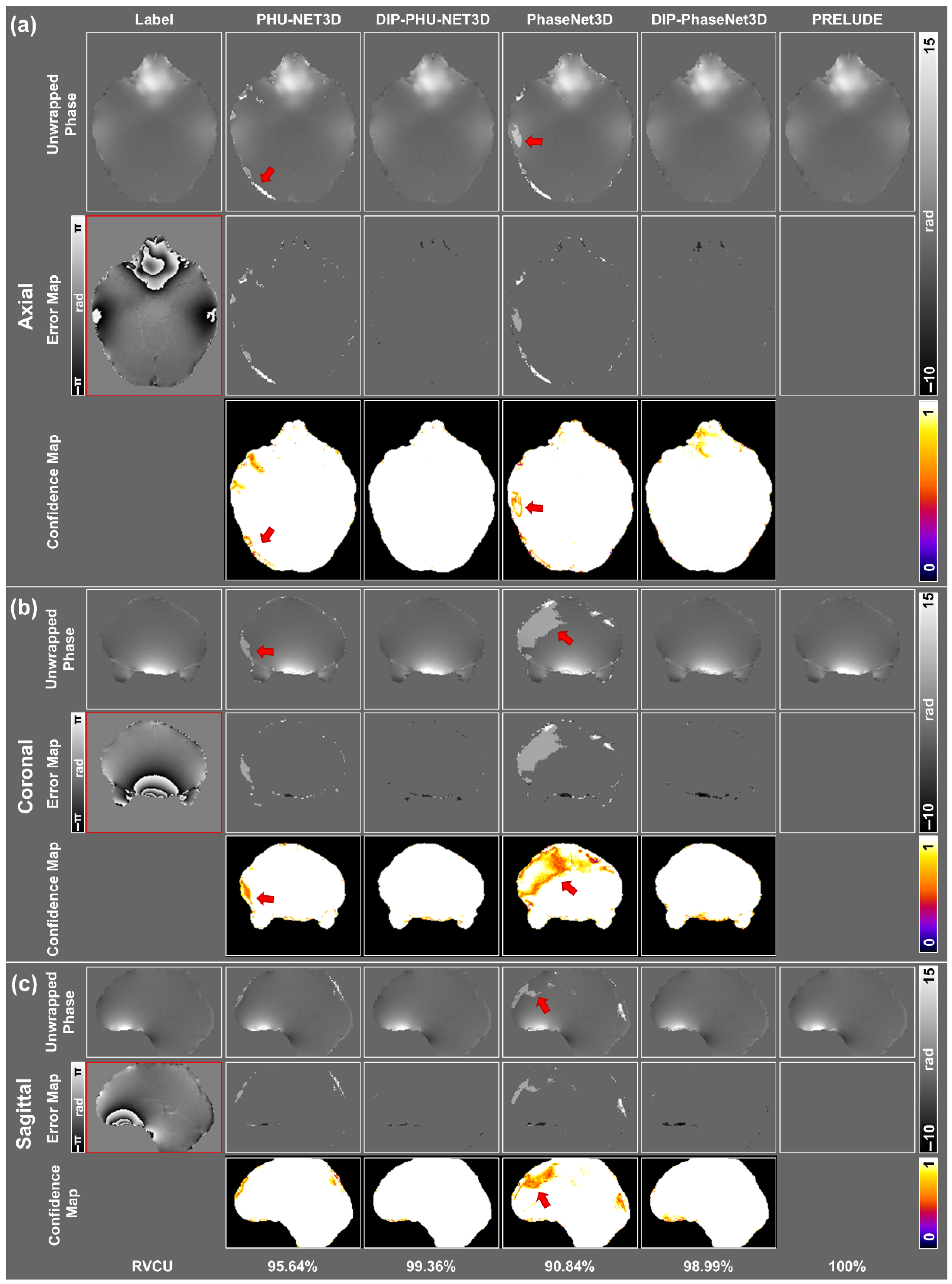
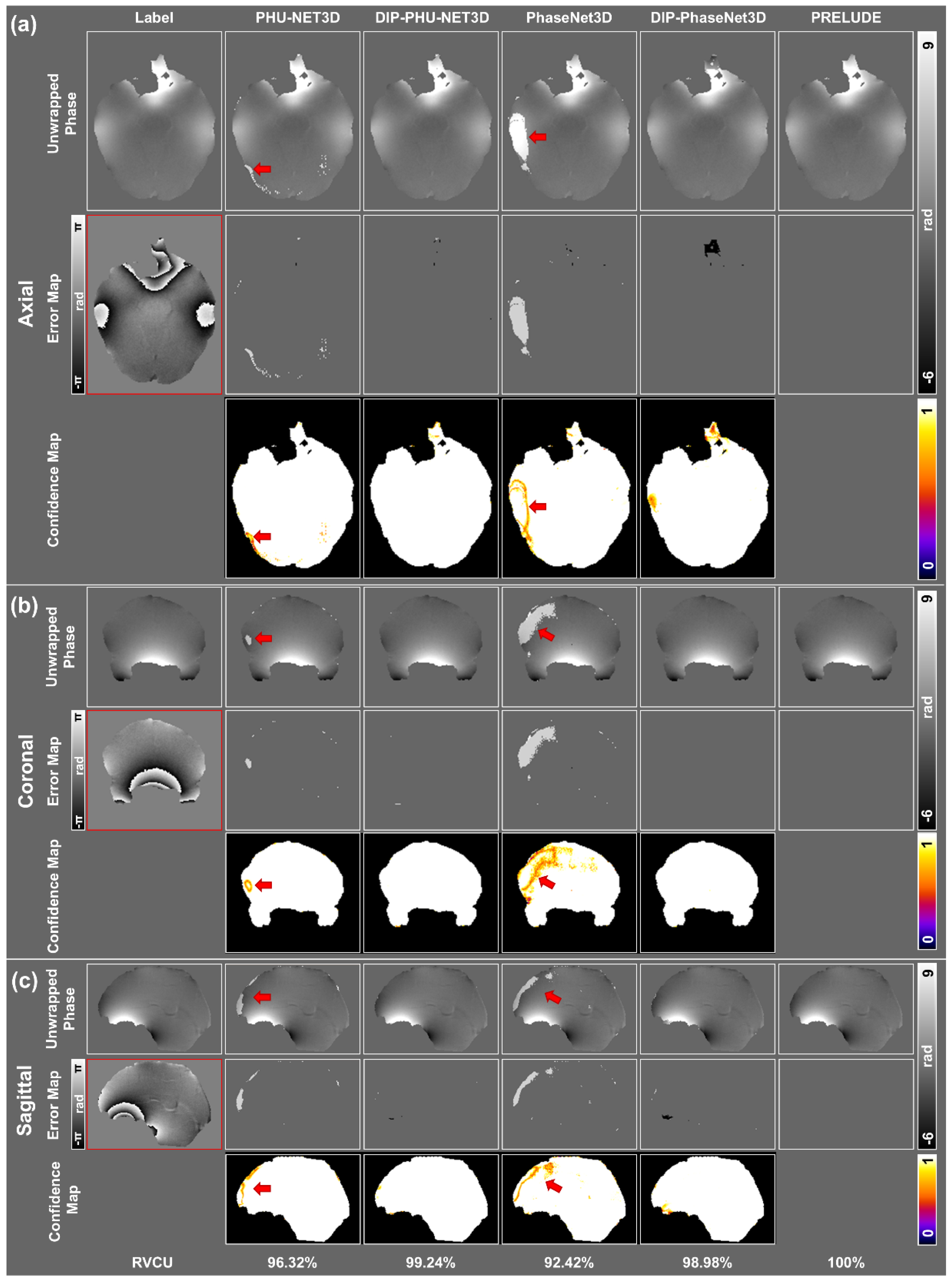
3.2. In Vivo Experiments

Figure 7 illustrates the unwrapped phases and their corresponding confidence map derived from an in vivo acquisition with TE = 5.8 ms. The presentation includes axial (Figure 7a) and coronal (Figure 7b) views. Line profiles are displayed in the third column of each view, crossing the regions with phase variations. Results from the PRELUDE were used as a gold-standard reference. The visual similarity between the outcomes of DIP-PHU-NET3D and PRELUDE is apparent, whereas initial results from PHU-NET3D and PhaseNet3D failed in the brainstem and cerebellum, as indicated by the red arrows. It is worth highlighting that DIP-PHU-NET3D successfully corrected the unsolved regions near the thalamus, as evident from visual observations in both axial and sagittal views. This is also confirmed in corresponding confidence maps and line profiles. Nevertheless, residual wrappings persist in the cerebellum, as pointed out by yellow arrow in the DIP-PHU-NET3D result. In contrast, DIP-PhaseNet3D displayed a different outcome that the misclassification in the cerebellum was fully rectified. However, regions adjacent to the sinus remained only partially solved, leading to the presence of discrete and abrupt phase values in the line profiles. Throughout the refinement process, DIP-PhaseNet3D expended 107 s, while DIP-PHU-NET3D consumed 130 s, both encompassing 200 iterations at a learning rate of 10⁻⁶. In contrast, PRELUDE notably required a longer duration of 330 s. Comparing to the gold-standard PRELUDE result, both DIP results performed better than their original networks, and DIP-PHU-NET3D has the highest SSIM of 0.9682 and lowest nMAE with 0.0158.

Figure 8 demonstrates the results of an in vivo experiment through five phase unwrapping methods using a TE of 10.6 ms (Figure 8a, axial and Figure 8b, coronal). Each view presents an unwrapped phase map and its corresponding confidence map in the left and middle columns, respectively. The right column features line profiles capturing phase variations. Similar to the observations made in the aforementioned subject with 5.8 ms TE, both DIP-PHU-NET3D and DIP-PhaseNet3D exhibited fewer misclassifications than initial results. In contrast, PHU-NET3D and PhaseNet3D were burdened by significant residual wrappings, evidenced by the decayed confidence values of approximately 0.5 along the boundaries of unresolved regions. Following the DIP processing, these figures experienced an elevation to around 1.0. Similar trends are observed in the line profiles, with both PHU-NET3D and PhaseNet3D exhibiting residual wrappings. In the case of PHU-NET3D, a discrete phase value was noticeable near the ear canal, while a persistently shifted value was present within the cerebellum. These inaccuracies in unwrapping were effectively rectified through the subsequent application of DIP processing. Comparing to the gold-standard PRELUDE result, DIP-PHU-NET3D achieved a higher SSIM, with 0.9589, and lower nMAE compared to the original PHU-NET3D results (SSIM of 0.9076 and nMAE of 0.0721). The PhaseNet3D results had the lowest SSIM (0.8373) and highest nMAE (0.1605) among the four learning-based methods. In terms of DIP processing durations, DIP-PhaseNet3D achieved an optimal outcome within 27 s over 50 iterations, while DIP-PHU-NET3D required 140 s across 200 iterations. Both DIP-PHU-NET3D and DIP-PhaseNet3D were executed using a learning rate that commenced at 10^-5 and decayed by 10% every 20 iterations. Despite PRELUDE results yielding a visually more precise absolute phase compared to the DIP results, the processing time for PRELUDE was significantly longer, at 605 s. Note that all five methods encountered challenges in regions with densely packed wrapping counts, specifically in areas adjacent to the sinus, which are pointed out by yellow arrows.

4. Discussion

Existing solutions present critical trade-offs: global optimizers like PRELUDE achieve gold-standard accuracy yet remain computationally expensive and fail for phase jumps > 2π in adjacent voxels. Additionally, PRELUDE’s computational efficiency and performance decrease significantly with increasing noise levels. Previous learning-based approaches (e.g., PhaseNet 2.0 and PHUnet) enable real-time processing but are constrained to 2D phase unwrapping only. To solve these issues, the proposed method presents a novel data generation and training approach to 3D phase data and, more importantly, refining the pre-trained models on individual cases during inference time with deep image prior with novel loss functions. DIP-UP specifically addresses four key limitations in the current phase unwrapping research: (1) the lack of generalizability in 2D-trained networks to 3D brain MRI structures, (2) poor noise robustness in conventional methods, (3) computational inefficiency in global optimization approaches, and (4) heavy dependency on labelled training data. We designed two frameworks and used DIP to post-process the original results. DIP was able to compensate for the misclassified regions in the original networks, as seen in the post-processed reconstructions. This improvement was observed upon both pre-trained networks, demonstrating the generalizability of DIP. The proposed method exhibited promising performance on both simulated and in vivo MR data. We selected the reconstructed unwrapped phase images before and after DIP and made comparison to the results obtained using a non-deep learning gold-standard method, PRELUDE. Both DIP methods demonstrated greater time efficiency than PRELUDE, assuming access to high-performance hardware such as the NVIDIA A100 GPU.

Previous research [37,38,39,43] has conclusively demonstrated the efficacy of DIP when applied to an untrained network with a simple architecture. DIP can effectively resolve ill-posed problems by revealing potential solutions and eliminating artifacts that deviate from the original image. In our investigation, we leveraged DIP to refine a pre-trained network through weight updates, resulting in significant improvements over the initial reconstructions. The initial results generated by the pre-trained network provided valuable insights for employing DIP, which helped to reduce the need for manual parameter tuning. The effectiveness of DIP for phase unwrapping depends on the design of the loss function. In our study, the synergistic combination of Laplacian and TV losses enhances the performance of pre-trained networks during subject-specific inference. The Laplacian loss enforces physical fidelity by encouraging the unwrapped phase to conform to the harmonic properties of the raw phase, derived from the underlying physical model. Meanwhile, the TV loss serves as an edge-aware regularizer, smoothing out local discontinuities caused by misclassified voxels without over-blurring meaningful edges. This dual mechanism helps to compensate for prediction errors made by the pre-trained networks and improves the overall quality and robustness of the unwrapped output. The improvement of DIP was also revealed visually in the voxel-wise confidence map. DIP results showcased the potential of refining pre-trained networks to eliminate the regions of uncertainty, thereby leading to a marked improvement in the overall quality of predictions.

We also compared the proposed DIP-based models to one iterative method, PRELUDE. PRELUDE, the conventional gold-standard phase unwrapping method, demonstrated high accuracy in our initial experiments, particularly in cases with relatively mild phase wrapping. We found that the DIP results were generalizable to diverse test data, as was the case with PRELUDE. However, some misclassified regions were caused by count mismatches or excess in the training set. While PRELUDE achieved good performance, it was computationally expensive, taking ~450 s for noiseless data and ~1300 s for noisy data. In contrast, the DIP-based reconstruction reduced the time to 50 s in both cases (100 iterations using an A100 GPU). PRELUDE makes assumptions about the prior distribution of the phase and always chooses the least likely candidate pair in the stage. This can lead to the algorithm getting stuck in a local minimum, resulting in incorrect results. Moreover, PRELUDE is known to suffer from degraded performance and increased failure rates in scenarios with severe wraps or regions near the sinuses. Its processing time can scale up to several hours when applied to full-resolution, 3D whole-brain GRE phase maps, especially from long echo time acquisitions. DIP-based methods, on the other hand, can learn the prior distribution from a training dataset, which can also improve the accuracy of the unwrapping results. Finally, the robustness to noise also helped to avoid extensive time consumption during the post-processing procedures. Future work will aim to further enhance DIP-UP’s generalizability to extremely challenging cases, such as low SNR, severe phase wrapping, and ultra-high-resolution datasets.

However, DIP-based methods have some limitations. First, DIP requires careful parameter tuning, such as for the iteration and learning rate, to guide the optimization process. The learning rate and iteration number directly affect the convergence speed, stability, and image quality, which may vary depending on the features of the raw phase, including wrapping counts and noise level. The training framework and the loss function may affect the parameters’ settings. Secondly, in comparison to traditional end-to-end Unet approaches, DIP proves time-intensive during the post-processing phase. This demands substantial computational resources, consequently constraining the feasibility of the proposed technique. On the contrary, DIP necessitated an extended overestimation period and the application of an early-stop mechanism to optimize prediction remains variable upon the iteration count. Third, the data-driven inference is bounded by the count number within the training sets. In this proposed method, the training data only covered nine wrapping counts, and the test data may exceed this range. Exceeded classes in the inference map could alter the data distribution, making the result misclassified. Finally, the proposed method was only tested on healthy data and has not been evaluated on patient data with haemorrhage or classification. Future work could focus on the training data with longer TEs (i.e., with more wrapping counts). In addition, the early-stopping criterion should be taken into consideration for further DIP-based study.

In summary, this study presents DIP-UP, a novel 3D phase unwrapping framework tailored for brain MRI, which refines pre-trained deep learning models using a DIP strategy during inference. Unlike existing learning-based methods that are typically constrained to 2D and require large, labelled datasets, DIP-UP operates in a fully 3D and label-free setting, enabling accurate and robust phase unwrapping across both simulated and in vivo data. Our approach demonstrates superior performance in high-noise conditions and outperforms conventional methods like PRELUDE in both noise resilience and computational efficiency. Moreover, the incorporation of physics-informed loss functions enables generalizability and adaptability to future extensions such as multi-echo phase imaging. These findings highlight DIP-UP as a promising tool for advancing clinically reliable and scalable phase processing in MRI.

References

1. Chen, Z.; Zhai, X.; Chen, Z. Proof of linear MRI phase imaging from an internal fieldmap. NMR Biomed. 2022, 35, e4741. [Google Scholar] [CrossRef] [PubMed]
2. Ong, F.; Cheng, J.Y.; Lustig, M. General phase regularized reconstruction using phase cycling. Magn. Reson. Med. 2018, 80, 112–125. [Google Scholar] [CrossRef] [PubMed]
3. Robinson, S.D.; Bredies, K.; Khabipova, D.; Dymerska, B.; Marques, J.P.; Schweser, F. An illustrated comparison of processing methods for MR phase imaging and QSM: Combining array coil signals and phase unwrapping. NMR Biomed. 2017, 30, e3601. [Google Scholar] [CrossRef]
4. Hasan, K.A. One-dimensional Hilbert transform processing for N-dimensional phase unwrapping. WSEAS Trans. Circuits Syst. 2006, 5, 783–789. [Google Scholar]
5. Barbieri, M.; Chaudhari, A.S.; Moran, C.J.; Gold, G.E.; Hargreaves, B.A.; Kogan, F. A method for measuring B0 field inhomogeneity using quantitative double-echo in steady-state. Magn. Reson. Med. 2023, 89, 577–593. [Google Scholar] [CrossRef] [PubMed]
6. Bechler, E.; Stabinska, J.; Wittsack, H.J. Analysis of different phase unwrapping methods to optimize quantitative susceptibility mapping in the abdomen. Magn. Reson. Med. 2019, 82, 2077–2089. [Google Scholar] [CrossRef]
7. Hanspach, J.; Bollmann, S.; Grigo, J.; Karius, A.; Uder, M.; Laun, F.B. Deep learning—Based quantitative susceptibility mapping (QSM) in the presence of fat using synthetically generated multi-echo phase training data. Magn. Reson. Med. 2022, 88, 1548–1560. [Google Scholar] [CrossRef]
8. Chavez, S.; Xiang, Q.-S.; An, L. Understanding phase maps in MRI: A new cutline phase unwrapping method. IEEE Trans. Med. Imaging 2002, 21, 966–977. [Google Scholar] [CrossRef]
9. Zhu, X.; Gao, Y.; Liu, F.; Crozier, S.; Sun, H. BFRnet: A deep learning-based MR background field removal method for QSM of the brain containing significant pathological susceptibility sources. Z. Med. Phys. 2022, 33, 578–590. [Google Scholar] [CrossRef]
10. Sun, H.; Wilman, A.H. Background field removal using spherical mean value filtering and Tikhonov regularization. Magn. Reson. Med. 2014, 71, 1151–1157. [Google Scholar] [CrossRef]
11. Gao, Y.; Xiong, Z.; Fazlollahi, A.; Nestor, P.J.; Vegh, V.; Nasrallah, F.; Winter, C. Instant tissue field and magnetic susceptibility mapping from MRI raw phase using Laplacian enhanced deep neural networks. NeuroImage 2022, 259, 119410. [Google Scholar] [CrossRef]
12. Fortier, V.; Levesque, I.R. Phase processing for quantitative susceptibility mapping of regions with large susceptibility and lack of signal. Magn. Reson. Med. 2018, 79, 3103–3113. [Google Scholar] [CrossRef]
13. Cheng, J.; Zheng, Q.; Xu, M.; Xu, Z.; Zhu, L.; Liu, L.; Han, S.; Chen, W. New 3D phase-unwrapping method based on voxel clustering and local polynomial modeling: Application to quantitative susceptibility mapping. Quant. Imaging Med. Surg. 2023, 13, 1550. [Google Scholar] [CrossRef] [PubMed]
14. Zhou, K.; Zaitsev, M.; Bao, S. Reliable two-dimensional phase unwrapping method using region growing and local linear estimation. Magn. Reson. Med. Off. J. Int. Soc. Magn. Reson. Med. 2009, 62, 1085–1090. [Google Scholar] [CrossRef] [PubMed]
15. Maier, F.; Fuentes, D.; Weinberg, J.S.; Hazle, J.D.; Stafford, R.J. Robust phase unwrapping for MR temperature imaging using a magnitude-sorted list, multi-clustering algorithm. Magn. Reson. Med. 2015, 73, 1662–1668. [Google Scholar] [CrossRef] [PubMed]
16. Loecher, M.; Schrauben, E.; Johnson, K.M.; Wieben, O. Phase unwrapping in 4D MR flow with a 4D single-step laplacian algorithm. J. Magn. Reson. Imaging 2016, 43, 833–842. [Google Scholar] [CrossRef]
17. Schofield, M.A.; Zhu, Y. Fast phase unwrapping algorithm for interferometric applications. Opt. Lett. 2003, 28, 1194–1196. [Google Scholar] [CrossRef]
18. Jenkinson, M. Fast, automated, N-dimensional phase-unwrapping algorithm. Magn. Reson. Med. Off. J. Int. Soc. Magn. Reson. Med. 2003, 49, 193–197. [Google Scholar] [CrossRef]
19. Karsa, A.; Shmueli, K. SEGUE: A speedy region-growing algorithm for unwrapping estimated phase. IEEE Trans. Med. Imaging 2018, 38, 1347–1357. [Google Scholar] [CrossRef]
20. Abdul-Rahman, H.S.; Gdeisat, M.A.; Burton, D.R.; Lalor, M.J.; Lilley, F.; Moore, C.J. Fast and robust three-dimensional best path phase unwrapping algorithm. Appl. Opt. 2007, 46, 6623–6635. [Google Scholar] [CrossRef]
21. Abdul-Rahman, H.; Arevalillo-Herráez, M.; Gdeisat, M.; Burton, D.; Lalor, M.; Lilley, F.; Moore, C.; Sheltraw, D. Robust three-dimensional best-path phase-unwrapping algorithm that avoids singularity loops. Appl. Opt. 2009, 48, 4582–4596. [Google Scholar] [CrossRef]
22. Véron, A.S.; Lemaitre, C.; Gautier, C.; Lacroix, V.; Sagot, M.-F. Close 3D proximity of evolutionary breakpoints argues for the notion of spatial synteny. BMC Genom. 2011, 12, 303. [Google Scholar] [CrossRef] [PubMed]
23. Wang, K.; Kemao, Q.; Di, J.; Zhao, J. Deep learning spatial phase unwrapping: A comparative review. Adv. Photonics Nexus 2022, 1, 014001. [Google Scholar] [CrossRef]
24. Huang, W.; Mei, X.; Wang, Y.; Fan, Z.; Chen, C.; Jiang, G. Two-dimensional phase unwrapping by a high-resolution deep learning network. Measurement 2022, 200, 111566. [Google Scholar] [CrossRef]
25. Zhang, T.; Jiang, S.; Zhao, Z.; Dixit, K.; Zhou, X.; Hou, J.; Zhang, Y.; Yan, C. Rapid and robust two-dimensional phase unwrapping via deep learning. Opt. Express 2019, 27, 23173–23185. [Google Scholar] [CrossRef] [PubMed]
26. Wang, K.; Li, Y.; Kemao, Q.; Di, J.; Zhao, J. One-step robust deep learning phase unwrapping. Opt. Express 2019, 27, 15100–15115. [Google Scholar] [CrossRef]
27. Gao, Y.; Zhu, X.; Moffat, B.A.; Glarin, R.; Wilman, A.H.; Pike, G.B.; Crozier, S.; Liu, F. xQSM: Quantitative susceptibility mapping with octave convolutional and noise-regularized neural networks. NMR Biomed. 2021, 34, e4461. [Google Scholar] [CrossRef]
28. Zhu, X.; Gao, Y.; Liu, F.; Crozier, S.; Sun, H. Deep grey matter quantitative susceptibility mapping from small spatial coverages using deep learning. Z. Für Med. Phys. 2022, 32, 188–198. [Google Scholar] [CrossRef]
29. Spoorthi, G.; Gorthi, S.; Gorthi, R.K.S.S. PhaseNet: A deep convolutional neural network for two-dimensional phase unwrapping. IEEE Signal Process. Lett. 2018, 26, 54–58. [Google Scholar] [CrossRef]
30. Spoorthi, G.; Gorthi, R.K.S.S.; Gorthi, S. PhaseNet 2.0: Phase unwrapping of noisy data based on deep learning approach. IEEE Trans. Image Process. 2020, 29, 4862–4872. [Google Scholar] [CrossRef]
31. Zhou, L.; Yu, H.; Pascazio, V.; Xing, M. PU-GAN: A one-step 2-D InSAR phase unwrapping based on conditional generative adversarial network. IEEE Trans. Geosci. Remote Sens. 2022, 60, 5221510. [Google Scholar] [CrossRef]
32. Goodfellow, I.; Pouget-Abadie, J.; Mirza, M.; Xu, B.; Warde-Farley, D.; Ozair, S.; Courville, A.; Bengio, Y. Generative adversarial networks. Commun. ACM 2020, 63, 139–144. [Google Scholar] [CrossRef]
33. Zhou, H.; Cheng, C.; Peng, H.; Liang, D.; Liu, X.; Zheng, H.; Zou, C. The PHU-NET: A robust phase unwrapping method for MRI based on deep learning. Magn. Reson. Med. 2021, 86, 3321–3333. [Google Scholar] [CrossRef]
34. Chen, Z.; Quan, Y.; Ji, H. Unsupervised deep unrolling networks for phase unwrapping. In Proceedings of the IEEE/CVF Conference on Computer Vision and Pattern Recognition, Seattle, WA, USA, 16–22 June 2024. [Google Scholar]
35. Yin, W.; Chen, Q.; Feng, S.; Tao, T.; Huang, L.; Trusiak, M.; Asund, A.; Zuo, C. Temporal phase unwrapping using deep learning. Sci. Rep. 2019, 9, 20175. [Google Scholar] [CrossRef] [PubMed]
36. Boroujeni, S.P.H.; Razi, A. Ic-gan: An improved conditional generative adversarial network for rgb-to-ir image translation with applications to forest fire monitoring. Expert Syst. Appl. 2024, 238, 121962. [Google Scholar] [CrossRef]
37. Ulyanov, D.; Vedaldi, A.; Lempitsky, V. Deep image prior. In Proceedings of the IEEE Conference on Computer Vision and Pattern Recognition, Salt Lake City, UT, USA, 18–23 June 2018. [Google Scholar]
38. Xiong, Z.; Gao, Y.; Liu, Y.; Fazlollahi, A.; Nestor, P.; Liu, F.; Sun, H. Quantitative susceptibility mapping through model-based deep image prior (MoDIP). NeuroImage 2024, 291, 120583. [Google Scholar] [CrossRef]
39. Yang, F.; Pham, T.-A.; Brandenberg, N.; Lütolf, M.P.; Ma, J.; Unser, M. Robust phase unwrapping via deep image prior for quantitative phase imaging. IEEE Trans. Image Process. 2021, 30, 7025–7037. [Google Scholar] [CrossRef]
40. Smith, S.M. Fast robust automated brain extraction. Hum. Brain Mapp. 2002, 17, 143–155. [Google Scholar] [CrossRef]
41. Liu, T.; Spincemaille, P.; De Rochefort, L.; Kressler, B.; Wang, Y. Calculation of susceptibility through multiple orientation sampling (COSMOS): A method for conditioning the inverse problem from measured magnetic field map to susceptibility source image in MRI. Magn. Reson. Med. Off. J. Int. Soc. Magn. Reson. Med. 2009, 61, 196–204. [Google Scholar] [CrossRef]
42. Liu, T.; Khalidov, I.; de Rochefort, L.; Spincemaille, P.; Liu, J.; Tsiouris, A.J.; Wang, Y. A novel background field removal method for MRI using projection onto dipole fields. NMR Biomed. 2011, 24, 1129–1136. [Google Scholar] [CrossRef]
43. Reddy, P.K.; Sudarshan, V.P.; Gubbi, J.; Pal, A. Structural-Mr Informed QSM Reconstruction Using Deep Image Prior. In Proceedings of the 2022 IEEE 19th International Symposium on Biomedical Imaging (ISBI), Kolkata, India, 28–31 March 2022; IEEE: Piscataway, NJ, USA, 2022. [Google Scholar] [CrossRef]
Figure 1. The generation pipeline of the DIP-UP training dataset, including raw phase, corresponding Laplacian map of raw phase, and count (label) calculation.
Information 16 00592 g001
Figure 2. The architecture of training step based on U-net architecture, incorporating the encoder sections (purple), middle layer (mandarin) and decoder (blue) sections.
Information 16 00592 g002
Figure 3. The scheme of DIP for refining the pre-trained network in phase unwrapping. Parameter space of the network (θ) is demonstrated as the blue surface. An initial wrapping count (K) is produced by the pre-trained network (θ) and optimized by DIP. The weights of θ are updated based on the loss () calculated on φn. The top left of the figure shows the simplified framework of θ. The number of feature maps (θn) is specified at the bottom of each block.
Information 16 00592 g003
Figure 4. Comparison of PHU-NET3D, DIP-PHU-NET3D, PhaseNet3D, DIP-PhaseNet3D, and PRELUDE on the simulated raw phase of brain tissue with TE = 3.0 ms, shown in (a) axial and (b) sagittal view. The red box delineates the raw phase. The unwrapped phase and difference map to the ground truth are shown in the first and second row in (ac). The corresponding confidence maps are shown in the third row. Misclassified regions are pointed out by red arrows.
Information 16 00592 g004
Figure 5. Three views of (a) axial, (b) coronal, and (c) sagittal results from the simulated raw phase of brain tissue with TE = 6.3 ms. The first and the second row represent the unwrapped phase and difference map relative to the ground truth. The corresponding confidence maps are shown in the bottom. The red arrows point to the incorrect unwrapped regions. The raw phase is encased within a red box.
Information 16 00592 g005
Figure 6. Comparison of five phase unwrapping methods on simulated brain tissue with 10 ms TE and noise with σ = 0.1. The three views are demonstrated in (ac). The boundaries of the raw phase are marked by a red box. The red arrows highlight the error regions. The corresponding confidence maps are shown on the bottom row of unwrapped phases and error maps.
Information 16 00592 g006
Figure 7. (a) Axial and (b) Coronal view from an in vivo subject, with TE = 5.8 ms. The absolute phases, relative error maps, and corresponding confidence map from five methods are shown from the first to the third second columns, respectively. The raw phase is encased within a red box. Densely wrapped regions near the sinus and cerebellum are highlighted in a yellow box. The profiles of the yellow lines crossing the phase-variant regions are plotted in the third column. The regions of misclassification are pointed out by red and yellow arrows, shown in both unwrapped phase and line profiles. Performance metrics relative to PRELUDE, including normalized mean absolute error (nMAE) and structural similarity index measurement (SSIM), of the learning-based methods are listed in the table below section (a).
Information 16 00592 g007
Figure 8. Results of five methods from an in vivo volunteer with TE = 10.6 ms, shown in (a) axial and (b) sagittal view. The error map indicates the difference between learning-based models and PRELUDE results. The confidence map corresponds to five methods that are shown in the right of absolute phase. The plotted line-profile reported the phase value the cross the yellow line. Misclassified areas are visually denoted using red arrows. Misclassified areas are visually denoted using red arrows and highlighted in the yellow boxes. Unsolved regions are pointed at by yellow arrows. Performance metrics of four learning-based methods relative to the PRELUDE method are shown in the table.
Information 16 00592 g008
Disclaimer/Publisher’s Note: The statements, opinions and data contained in all publications are solely those of the individual author(s) and contributor(s) and not of MDPI and/or the editor(s). MDPI and/or the editor(s) disclaim responsibility for any injury to people or property resulting from any ideas, methods, instructions or products referred to in the content.