Limited Data Availability in Building Energy Consumption Prediction: A Low-Rank Transfer Learning with Attention-Enhanced Temporal Convolution Network

Abstract

Building energy consumption prediction (BECP) is the essential foundation for attaining energy efficiency in buildings, contributing significantly to tackling global energy challenges and facilitating energy sustainability. However, while data-driven methods have emerged as a crucial method to solving this complex problem, the limited availability of data presents a significant challenge to model training. To address this challenge, this paper presents an innovative method, named Low-Rank Transfer Learning with Attention-Enhanced Temporal Convolution Network (LRTL-AtTCN). LRTL-AtTCN integrates the attention mechanism with temporal convolutional network (TCN), improving the ability of extracting global and local dependencies. Moreover, LRTL-AtTCN combines low-rank decomposition, reducing the number of parameters during the transfer learning process with similar buildings, which can achieve better transfer performance in the limited data case. Experimentally, we conduct a comprehensive evaluation across three forecasting horizons—1 week, 2 weeks, and 1 month. Compared to the horizon-matched baseline, LRTL-AtTCN cuts the MAE by 91.2%, 30.2%, and 26.4%, respectively, and lifts the 1-month R² from 0.8188 to 0.9286. On every horizon it also outperforms state-of-the-art transfer-learning methods, confirming its strong generalization and transfer capability in BECP.

1. Introduction

Nowadays, building energy consumption represents roughly 34% of global final energy use, while carbon dioxide emissions associated with buildings account for 37% of total global emissions [1]. The primary objective of enhancing building energy efficiency is to optimize energy utilization and reduce unnecessary consumption, especially for large public buildings. Generally, achieving energy efficiency in buildings mainly depends on the implementation of effective building management strategies [2], while the development of these strategies is contingent upon building energy consumption prediction (BECP), which plays a pivotal role in understanding and anticipating dynamic changes in energy consumption patterns and guiding energy management decisions. Effective BECP is a method that analyzes and predicts the dynamics of energy use and assists managers in anticipating trends in energy demand and optimizing energy allocation, significantly reducing the overall level of energy consumption in buildings [3]. Personalized control within BECP facilitates the intelligent and precise operation of energy-consuming equipment, thereby ensuring the stable functioning of building systems while maintaining interior comfort. Moreover, BECP functions as a valuable auxiliary tool in the realms of intelligent control [4], demand-side management strategies [5], and fault detection and diagnosis [6], exhibiting a diverse range of applications across these domains.

There are two main kinds of methods for BECP: physics-based modeling methods and data-driven methods. Physics-based modeling methods involve creating explicit models based on parameters that reflect the intrinsic characteristics of the building, enabling the prediction of its energy consumption [2]. However, the construction of physical models for buildings necessitates a substantial set of detailed operational parameters—including thermophysical characteristics, energy equipment specifications, and system settings such as occupancy schedules and air conditioning zoning—while also relying heavily on extensive measurement data to ensure model accuracy [7]. Consequently, the implementation of physics-based modeling methods faces significant challenges in achieving accurate predictions. In contrast, data-driven methods utilize machine learning to predict building energy consumption by developing models based on extensive historical data [2], resulting in substantial advancements in the field of BECP. The most common data-driven methods can be categorized into two primary kinds: statistical learning methods and deep learning methods. The field of statistical learning applied in BECP encompasses a variety of techniques, including Support Vector Regression (SVR) [8], Multiple Linear Regression(MLR) [9], Random Forest (RF) [10], and Extreme Gradient Boosting (XGBoost) [11], and so on. These methods provide several advantages, including low computational resource requirements, rapid training and prediction speeds, and high interpretability of the models. Meanwhile, deep learning methods employed in BECP can be categorized into several types: Recurrent Neural Networks (RNNs) [12], such as LSTM [13] and GRU [14], are particularly effective for processing sequential data and adept at capturing both long- and short-term dependencies; Convolutional Neural Networks (CNNs) [15], such as Temporal Convolutional Network (TCN) [16], excel at extracting local hidden features and managing short-term fluctuations; and Attention-based methods [17], are proficient in processing long sequences of data and capturing global dependencies. Due to the powerful ability of feature learning, deep learning has achieved remarkable results and has been widely applied in BECP. However, like statistical learning methods, deep learning relies heavily on substantial historical data. In scenarios where such data is limited—such as in newly constructed buildings or in the absence of a comprehensive energy monitoring system—this limitation poses a significant barrier to the effective implementation of BECP.

The challenge of limited data availability has become a central focus in research related to BECP. To address this problem, several perspectives can be considered. Data augmentation [18] and synthetic data generation [19] have proven to be viable strategies for enhancing the quality and diversity of datasets, thereby improving the models’ prediction performance, and addressing the issue of limited data availability. However, these methods often rely on techniques like noise injection and data recombination, which may introduce inconsistencies and fail to accurately represent real-world conditions, thus hindering the model’s applicability in practical scenarios. Moreover, Transfer learning [20] is an effective method for addressing the issue of limited data availability in BECP. By leveraging data from different buildings or regions, transfer learning applies the acquired knowledge to the target domain with limited data, thereby reducing the dependency on large-scale datasets. In practical applications, transfer learning can swiftly adapt to the variations in energy consumption characteristics of new buildings or regions, maintaining high prediction accuracy in diverse and dynamic environments. Despite the increasing use of transfer learning in BECP, existing methods often require extensive parameter updates to adapt to the target domain, which hinders practical deployment, especially under limited data scenarios [21]. Furthermore, cross-domain discrepancies—stemming from differences in HVAC configurations, occupant behavior, and energy management strategies—introduce significant domain shifts, compromising generalization and increasing the risk of overfitting [20]. These challenges reveal two major gaps in current BECP methods: (1) the lack of lightweight and adaptive transfer mechanisms that reduce parameter overhead. (2) insufficient robustness to domain shifts under data limited.

To address overparameterization associated with traditional transfer learning, mitigating inter-domain discrepancies among buildings, and to enhance the performance of BECP in scenarios characterized by limited data availability, we propose a Low-Rank Attention-Enhanced Temporal Convolutional Transfer Learning method (LRTL-AtTCN). By integrating the attention mechanism with the local feature extraction capability of the Temporal Convolutional Network (TCN), we establish a temporal feature learning framework with the ability to model global dependencies. This framework addresses the inherent defect of the limited receptive field of TCN, thereby enhancing the feature extraction ability of the model. Meanwhile, the low-rank transfer learning framework we propose can reduce the parameter redundancy while maintaining the cross-domain invariant features, and this characteristic has been verified through experiments. For the first time, LRTL systematically expounds how the low-rank constraint can simultaneously achieve the dual objectives of minimizing the differences across building domains and preserving key knowledge during the transfer process, providing a viable solution to these challenges. In summary, the LRTL-AtTCN framework employs an attention-enhanced TCN architecture, which captures both local and global temporal dependencies simultaneously through a dynamic weighting mechanism; the low-rank transfer mechanism significantly reduces the parameter transfer cost while maintaining the prediction performance across different building domains. The principal contributions of this paper are as follows:

• We propose integrating the attention mechanism with TCN, named AtTCN. AtTCN enhances the model’s ability to dynamically capture global dependencies with the attention mechanism, addressing the limitations of TCN’s local receptive field, and capturing both local and global hidden features more effectively.
• By introducing low-rank decomposition, we propose a novel transfer learning-based AtTCN method, named LRTL-AtTCN, which significantly reduces the number of parameters during the transfer learning process and achieves better prediction performance in conditions of limited data, demonstrating great adaptability across different building types.
• We evaluate LRTL-AtTCN, focusing on its performance in BECP in the source domain and the target domain with limited data, and specifically investigate the impact of the experimental results of the attention mechanism and low-rank decomposition. The code in this paper is available at https://github.com/Fechos/LRTL-AtTCN (accessed on 21 May 2025).

The paper is organized as follows. Section 1 introduces the background and motivation of building energy consumption prediction. Section 2 reviews existing work, including physics-based models, data-driven methods, and methods for addressing data scarcity. Section 3 formally defines the problem setting, and describes the proposed methodology, including data preprocessing, feature engineering, source domain model training, and the low-rank transfer learning framework. Section 4 presents the experimental setup, evaluation metrics, and result analysis. Finally, Section 5 concludes the paper and outlines potential future directions.

2. Related Works

2.1. Physics-Based Modeling Methods

BECP, particularly regarding cooling and heating demands, is typically computed using physics-based models that adhere to the energy balance principle, and commonly employed analysis tools for modeling include TRNSYS [22] EnergyPlus [23], DOE-2 [24], Dymola [25], and IDA-ICE [26]. The theoretical foundation of physics-based models is notably precise, and their detailed modeling processes facilitate a comprehensive analysis of all facets of a building’s energy consumption. However, these models necessitate a substantial number of input variables and parameters, leading to a complex and time-consuming settings. Additionally, the challenges related to data collection further complicate the modeling process. Despite the numerous methods that researchers have explored to mitigate these limitations, with data-driven methods being a prominent example [27], physical models continue to face significant challenges in practical applications.

2.2. Data-Driven Methods

In the field of BECP, statistical learning methods have played a crucial role in developing various solutions by optimizing feature engineering and employing other techniques. Ngo et al. [28] developed a WIO-SVR model for multi-step BECP, optimizing SVR hyperparameters through the GWO algorithm to enhance accuracy. Fan and Ding [29] proposed an MNR model for short-term cooling load prediction in public buildings, enhancing accuracy through the selection and calibration of key variables. Although the above-mentioned methods have achieved significant advancements in enhancing the accuracy and reliability of BECP, the limitations of statistical learning methods in handling high-dimensional data and modeling complexity may result in insufficient model adaptability, when confronted with intricate and dynamic building environments.

Meanwhile, the advent of deep learning has enabled models to discern intricate characteristics of time series more effectively, thereby paving the way for an abundance of novel methods. He et al. [30] introduced a fusion estimation method for air conditioning load prediction that combines particle filtering (PF) and LSTM with a back-propagation neural network (BP), constructing a state-space model, and integrating PF for load prediction. Le et al. [31] developed the EECP-CBL model for electrical energy consumption prediction, which combines CNN and a bidirectional long- and short-term memory (Bi-LSTM) network to extract pertinent hidden features and make predictions in both the forward and backward states of a time series. Lara-Benítez et al. [15] presented a deep learning model based on TCN for predicting electricity demand and EV charging station power demand in Spain. Cen et al. [32] introduced the PatchTCN-TST model, which fuses the Patch, TCN, and Time Series Transformer (TST) to predict multiple electrical loads and indoor environmental data at the building level. Li et al. [33] proposed a transformer-based building load prediction model aimed at enhancing the precision of building cooling load prediction by leveraging time series data through an encoding-decoding structure and an attention mechanism. Alsmadi et al. [34] proposes a novel hybrid CNN-LSTM-Attention model that effectively integrates Heating Degree Days (HDD) and Cooling Degree Days (CDD) to enhance day-ahead electricity demand forecasting in Australia, demonstrating superior accuracy over traditional methods by capturing nonlinear temperature–consumption relationships through spatial-temporal feature extraction and attention mechanisms. Chen et al. [35] proposed the Attention-TCN-LSTM model by integrating TCN with LSTM and incorporating an attention mechanism to improve 1 h single-step and 8 to 24 h multi-step prediction accuracy in energy storage systems. This method effectively reduced prediction errors and improved stability, addressing the limitation of conventional models in handling multiple time scales. Liu et al. [36] proposed a parallel-structured TCN-LSTM hybrid model that combines TCN and LSTM via a tensor concatenation module and applies a Savitzky–Golay filter to smooth wind speed data, aiming to enhance wind power prediction while reducing model complexity.

However, these methods heavily rely on extensive historical data, which poses significant limitations in BECP with limited data availability.

2.3. Methods for Handling Limited Data Availability

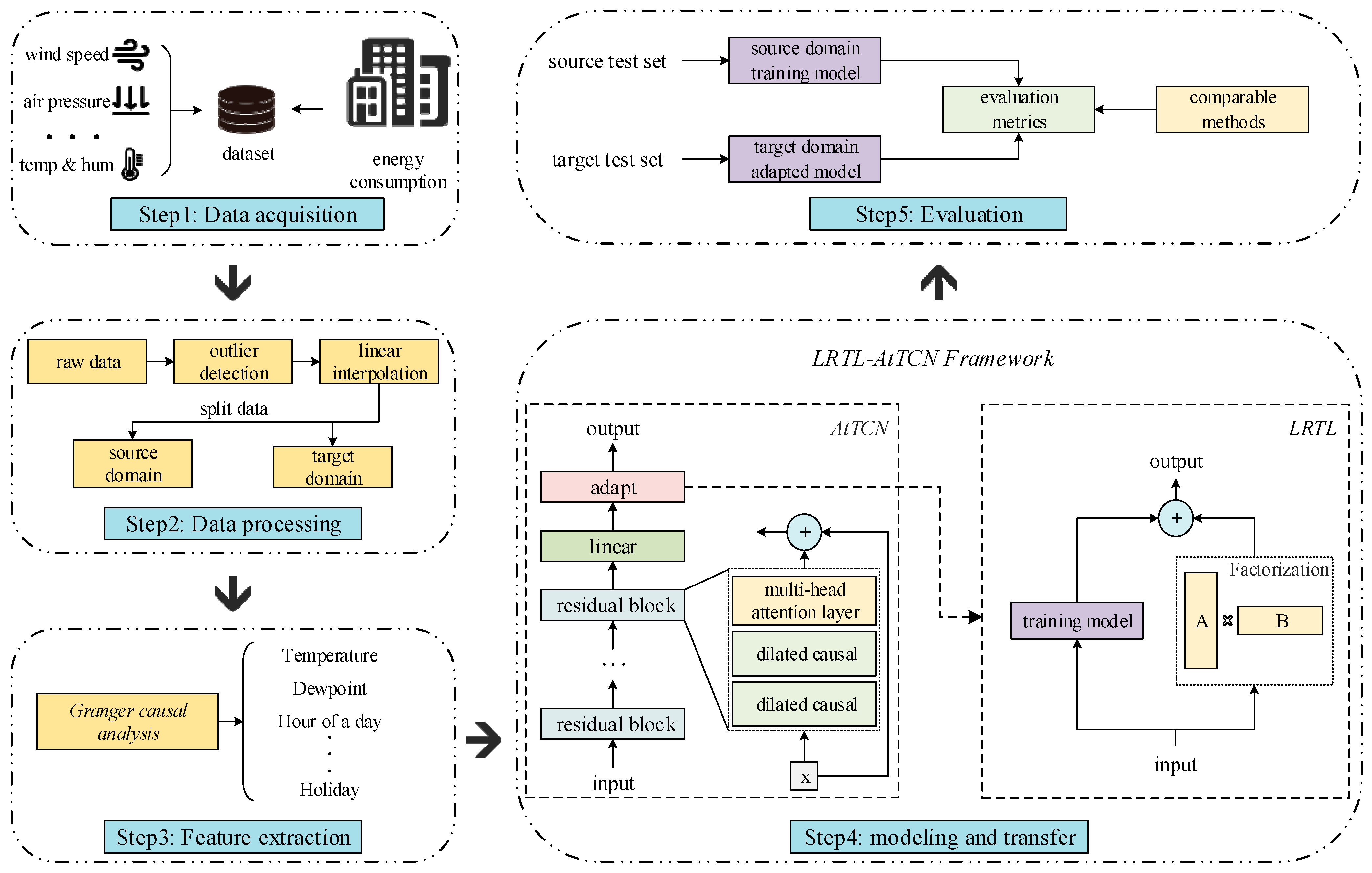
To address the challenge of limited data availability in BECP, researchers have undertaken extensive investigations and explored various strategies. Bandara et al. [37] proposed a data-enhanced global predictive modeling (GFM) method that, by utilizing data augmentation in conjunction with merged training and transfer learning, aims to mitigate the limitation of time series data. Fekri et al. [38] propose a parallel prediction method using generative adversarial nets (GANs) to augment data, blending real and artificial data to enhance model training. Gao et al. [39] proposed a transfer learning method that, by combining a sequence-to-sequence (seq2seq) with a two-dimensional convolutional neural network (2D CNN) and also using fine-tuning, aims to improve prediction accuracy in data-limited scenarios. Ye et al. [40] proposes a Relationship-Aligned Transfer Learning (aRATL) algorithm to address the challenge of limited training data in time series predicting by aligning relationships between source and target models, through a selective knowledge transfer process. Zang et al. [41] propose AdaRNN-DCORAL, combining adaptive prediction with domain adaptation techniques to enhance prediction accuracy. The above-mentioned methods have made considerable progress in addressing the issue of limited data availability from multiple perspectives. Hua et al. [42] introduces an energy consumption estimation method for electric vehicles (EVs) that leverages transfer learning to address the challenge of insufficient data. By transferring knowledge from internal combustion engine vehicles and hybrid electric vehicles, the proposed method effectively utilizes existing data to enhance the accuracy of energy consumption estimation. Xing et al. [43] explores the use of transfer learning for building energy consumption prediction, proposing a method that identifies similar source buildings and leverages weather parameters for both short-term and long-term predictions, showing significant improvements in accuracy compared to models using only target building data. Li et al. [44] proposed the LSTM-DANN-CDI hybrid strategy, which integrates transfer learning with coarse data incremental learning, to address the performance degradation of energy prediction models caused by data scarcity in newly built or information-poor buildings. Kamalov et al. [45] proposed an electricity forecasting method based on zero-shot transfer learning by training an NBEATS model on a large and diverse time series dataset, addressing the lack of problem-specific data in medium-term power generation forecasting. Chen et al. [46] proposed an ultra-short-term wind power prediction method combining stacking and transfer learning, using PCA for dimensionality reduction and an ensemble of various recurrent neural networks to address the low accuracy of single models.

Table 1. Overview of Modeling Methods and Data-Limited Solutions in BECP.

Category	Tools/Methods	Key Features	Limitations
Physics-based Modeling	TRNSYS [22], EnergyPlus [23], DOE-2 [24], Dymola [25], IDA-ICE [26]	Based on energy balance principles; precise and detailed building energy consumption modeling	Requires large number of input parameters; complex setup; difficult data collection
Statistical Learning	WIO-SVR [28], MNR [29]	Optimizes feature engineering; uses algorithms for improved accuracy	Limited capability for high-dimensional and complex data; insufficient adaptability
Deep Learning	PF+LSTM+BP [30], EECP-CBL [31], TCN [15], PatchTCN-TST [32], Transformer-based [33], CNN-LSTM-Attention [34], Attention-TCN-LSTM [35], TCN-LSTM hybrid [36]	Captures complex temporal features; integrates multiple network architectures and attention mechanisms	Heavy reliance on large historical datasets; limited performance with scarce data
Data Augmentation	GFM + Transfer Learning [37], GAN-based augmentation [38]	Augments data by generating synthetic samples; merges datasets to enrich training data	Synthetic data quality may affect model generalization; still needs domain alignment
Transfer Learning	Seq2seq + 2D CNN [39], aRATL [40], AdaRNN-DCORAL [41], LSTM-DANN-CDI [44], Zero-shot NBEATS [45], Stacking + Transfer Learning [46] et al.	Applies knowledge transfer, incremental learning, domain adaptation to leverage related tasks	Domain discrepancies between buildings, especially HVAC and occupant behavior, reduce transfer efficiency; need better transfer strategies

provides an overview of various modeling methods and solutions designed to address data limitations in BECP. In summary, BECP has been addressed by a variety of methods, including physics-based modeling, statistical learning, deep learning, data augmentation, and transfer learning, which each exhibit inherent limitations that constrain their effectiveness and generalizability in practical scenarios. Physics-based models, though accurate, require extensive input parameters and complex setups. Statistical learning methods face challenges with high-dimensional, complex data, limiting adaptability. Deep learning captures temporal dependencies well but depends heavily on large datasets and underperforms in data-limited scenarios. Data augmentation mitigates scarcity by generating synthetic samples, yet data quality and domain alignment issues persist. Transfer learning leverages related tasks effectively but suffers from high adaptation costs and poor robustness to domain discrepancies, especially due to variability in HVAC systems and occupant behavior.

In this paper, we enhance the TCN model by incorporating an attention mechanism to improve its ability to capture global temporal features, thereby addressing the limitation of standard TCNs in modeling long-range dependencies. Meanwhile, to address the common issue of data scarcity in building energy consumption prediction and overcome the limitations of existing transfer learning methods—namely, the high cost of parameter adaptation and poor robustness to cross-domain discrepancies—we introduce a low-rank decomposition strategy. By factorizing the model parameters into two low-rank matrices, this method significantly reduces the number of parameters that need to be updated during transfer, while preserving critical information from the source domain and suppressing redundant features. As a result, it effectively mitigates distributional differences between source and target domains and enhances the model’s generalization and adaptability under data-limited conditions.

3. Methodology

3.1. Problem Statement

BECP represents a typical time series prediction problem focused on predicting future energy consumption trends based on existing historical data. By capturing the time series features of building energy consumption, the model offers a scientific foundation for energy management and optimization, facilitating more efficient energy control and promoting sustainable development.

Time series predicting can be described as follows: given the historical time series $D_{1:t}=\left({\mathit{X}}_{1:t},{\mathit{y}}_{1:t}\right),{\mathit{X}}_{1:t}\in {\mathbb{R}}^{t \times m},{\mathit{y}}_{1:t}\in {\mathbb{R}}^{t \times 1}$, the future time series is then predicted, where $t$ is the length of the historical time series and $m$ is the number of external features. External features, also known as exogenous features or external inputs, encompass variables relevant to the target time series but not directly derived from its historical data. These features generally capture external environmental conditions and timestamp elements, including meteorological parameters (e.g., temperature, relative humidity, atmospheric pressure) and temporal attributes (e.g., specific dates, day of the year, holiday status). The information provided by these external features plays a critical role in enhancing the predictive accuracy and robustness of models associated with the target time series. In the field of BECP, ${\mathit{X}}_{1:t}$ represents external features series of building consumption data, and ${\mathit{y}}_{1:t}$ is building consumption series. With modeling $P\left(\left({\mathit{y}}_{t+1:t+\Omega }\right)|\left({\mathit{X}}_{1:t},{\mathit{y}}_{1:t}\right)\right)$, it allows us to make predictions about future values, where $\Omega$ denotes the prediction horizon, defined as the number of future time steps over which a forecasting model generates predictions.

In this paper, we employ transfer learning to address the challenge of limited data availability in BECP. Transfer learning [20] is an effective technique for improving the performance of a target domain model through transfer knowledge from the source domain that, while disparate, is relevant to the target domain. In this paper, we designate buildings with abundant data as the source domain and new buildings in similar environments, or those with limited data, as the target domain. By utilizing transfer learning, we aim to transfer the knowledge acquired in the source building domain to enhance prediction performance in the target building domain.

The transfer learning in building energy prediction is defined as follows: assuming there are source and target building domains. The source building domain data is defined as follows: $D^S=\left({\mathit{X}}_{1:t^S}^S,{\mathit{y}}_{1:t^S}^S\right)$, where ${\mathit{X}}_{1:{\mathit{t}}^{\mathit{S}}}^{\mathit{S}}$ is the external features series of the source building domain, ${\mathit{y}}_{1:t^S}^S$ is the source building consumption series, and $t^S$ is the source domain length of historical data. The target building domain data is defined as follows: $D^T=\left({\mathit{X}}_{1:t^T}^T,{\mathit{y}}_{1:t^T}^T\right)$, where ${\mathit{X}}_{1:{\mathit{t}}^{\mathit{T}}}^{\mathit{T}}$ is external features series of the target building domain, ${\mathit{y}}_{1:t^T}^T$ is the target building consumption series, and $t^T$ is the target domain length of historical data, where $t^T$ is considerably shorter than $t^S$ in transfer learning.

The objective is to enhance the prediction capability of ${\mathit{y}}_{1:t^T}^T$ with respect to the target building domain $D^T$ by leveraging the knowledge embedded in the source building domain $D^S$. Given a source building domain model $f^S:{(\mathit{X}}_{1:{\mathit{t}}^{\mathit{S}}}^{\mathit{S}},{\mathit{y}}_{1:t^S}^S)\to ({\mathit{y}}_{t^S+1:t^S+\Omega }^S)$, the objective is to learn a target building domain model $f^T:{(\mathit{X}}_{1:{\mathit{t}}^{\mathit{T}}}^{\mathit{T}},{\mathit{y}}_{1:t^T}^T)\to ({\mathit{y}}_{t^T+1:t^T+\Omega }^T)$, where $f^T$ minimizes the prediction error in the target building domain by effectively utilizing the information from the source building domain:

$$f^T=\underset{f^T}{argmin}(E_{{(\mathit{X}}_{1:t^T}^T,{\mathit{y}}_{1:t^T}^T)~D^T}(\mathcal{L}\left(f^T\right))+\lambda E_{{(\mathit{X}}_{1:t^S}^S,{\mathit{y}}_{1:t^S}^S)~D^S}(\mathcal{L}\left(f^S\right)))$$

(1)

where $\mathcal{L}\left(\cdot \right)$ denotes the loss function, and $\mathsf{\lambda }$ is the hyperparameter, which can balance the losses between the source building domain and the target building domain.

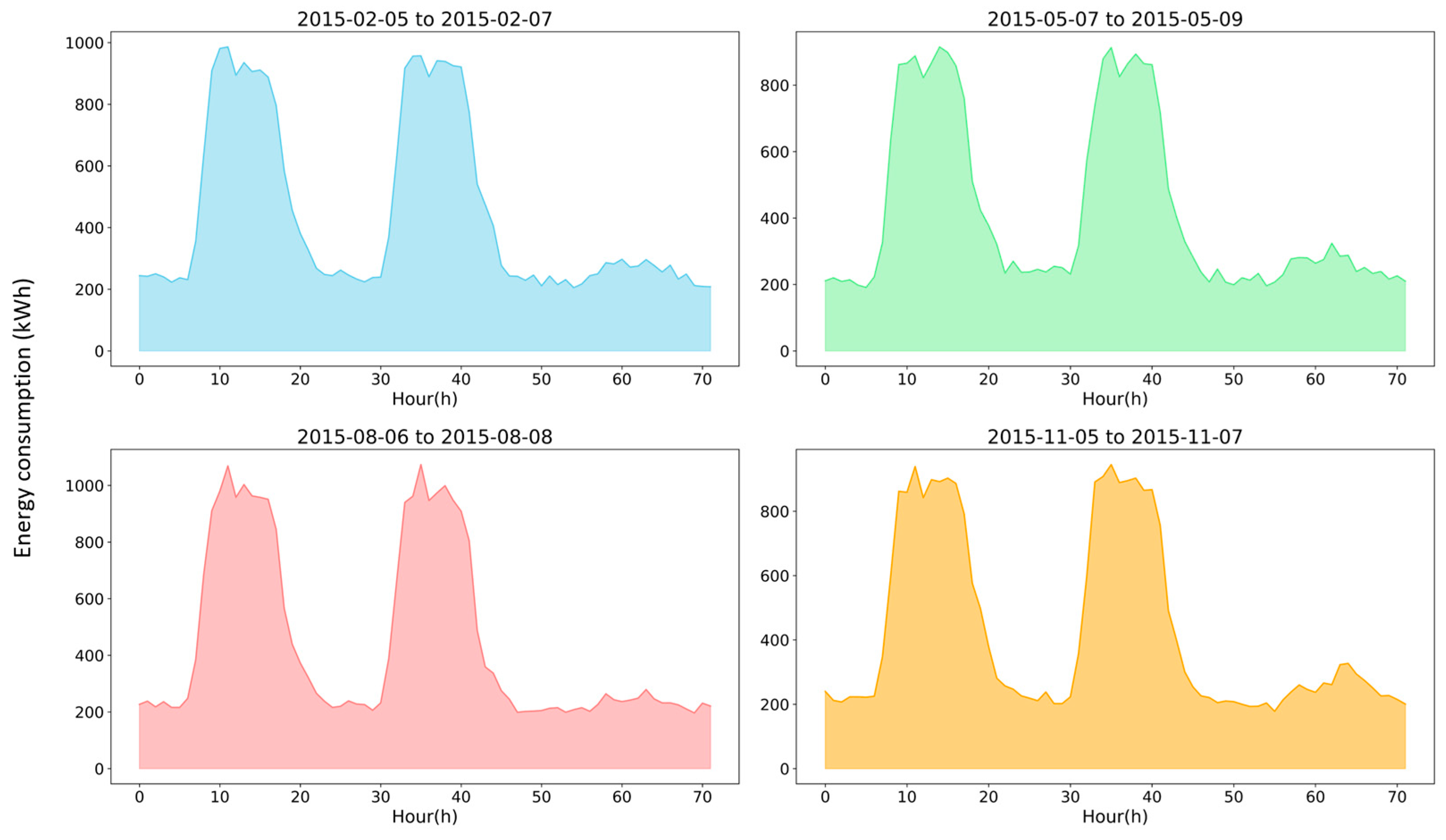
3.2. Data Processing

The overall framework of method in this paper is shown in Figure 1. It includes the following five steps: (1) Step 1: data acquisition. Energy consumption data in this paper were collected from several office buildings in Shanghai, China, and the weather data were collected from a weather station located within 5 km of the office. (2) Step 2: data processing. Statistical methods are employed to identify and process outliers in energy consumption data, thereby ensuring the accuracy and completeness of the dataset. Furthermore, the pertinent data are normalized to eliminate discrepancies between different scales and enhance the efficacy of model training. (3) Step 3: feature extraction. The data features were selected utilizing Granger causality analysis, which examines the causal relationship between external features and energy consumption. This method was employed to identify the key features that exert a substantial influence on energy consumption prediction. (4) Step 4: modeling and transfer. We utilize AtTCN for training of the source building domain and save the optimal model. Subsequently, we employ LRTL to transfer the trained model to the small-scale dataset on the target building domain, which enables the transfer of knowledge from the source building domain to the target building domain. (5) Step 5: evaluation: A comparative analysis is conducted between the source building domain and the target domain against other methods, with further performance evaluation of LRTL-AtTCN in Experiments and analysis.

A dataset of energy consumption from air-conditioned buildings was analyzed, derived from several office buildings in Shanghai, China, which vary in factors such as building area and HVAC system (Dataset source: Prof. Peng Xu’s group, School of Mechanical and Energy Engineering, Tongji University—De ang Technology, https://mp.weixin.qq.com/s/h9L0MFOQG5SghEZeDu92EA, accessed on 21 May 2025). The data was collected from 1 January 2015, at 12:00 a.m. to 31 December 2016, at 11:00 p.m., and sampled intervals were one hour. Due to a lack of data collection on 29 February 2016, the total number of observed samples for each office building amounted to 17,520. Apart from the energy consumption data of the buildings, the dataset encompasses meteorological information within a 5 km radius of each building, including variables such as temperature, dew point, relative humidity, air pressure, and wind speed. Additionally, the inclusion of timestamp features is shown to influence energy consumption features. These timestamp features are derived from the time series energy consumption data and encompass the hour of the day, the day of the week, the day of the month, the day of the year, the month of the year, the week of the year, and holiday status. The features previously delineated are referred to as external features used for energy consumption prediction, as mentioned in the Problem statement. The features are described in

Table 2. Features information.

Feature	Type	Range	Unit
building energy consumption	continuous	$[0,1000]$	kWh
temperature	continuous	$\left[-7,40\right]$	°C
dew point	continuous	$[-20,30]$	°C
relative humidity	continuous	$\left[13,100\right]$	%
air pressure	continuous	$[900,1100]$	Pa
wind speed	continuous	$\left[0,43.2\right]$	m/s
month of the year	categorical	$\left[1,2\cdots 12\right]$	-
day of the year	categorical	$\left[1,2\cdots 366\right]$	-
day of the month	categorical	$\left[1,2\cdots 31\right]$	-
day of the week	categorical	$\left[1,2\cdots 7\right]$	-
hour of the day	categorical	$\left[1,2\cdots 24\right]$	-
season	categorical	$[1,2,3,4]$	-
holiday status	categorical	$\left[0,1\right]$	-

.

This study investigates a representative energy consumption curve from the dataset, aiming to uncover characteristic consumption patterns and temporal dynamics. Figure 2 presents four subplots, each depicting the load curves from Thursday to Saturday across different seasons, where the horizontal axis in each subplot represents the time axis, while the vertical axis corresponds to energy consumption data. These subplots illustrate the seasonal variations in energy consumption, which demonstrate that energy consumption patterns remain unaffected by seasonal factors.

Figure 3 illustrates the differences in energy consumption patterns across weekdays, non-working days, and holidays, highlighting the variations in energy usage among these categories. By comparing the load curves for weekdays, non-working days, and holidays, the subplot reveals the influence of occupancy and operational patterns on energy consumption.

The presence of unidentified variables during the data collection and transmission stages can lead to the introduction of outliers and missing values in the dataset. To ensure precision performance and dependability of the model training process, it is essential to preprocess the data. We carefully identify and address any outliers within the dataset to maintain its quality. First, the distribution of values for each feature is checked using the interquartile range (IQR) method, which helps determine the range of outliers by calculating the upper and lower quartiles. For the identified outliers, we employ various processing strategies, including the removal of outliers that significantly deviate from the normal range, the use of linear interpolation to fill in missing values, and the truncation of extreme outliers.

3.3. Feature Engineering

Feature engineering involves developing meaningful features to serve as inputs for a model. To determine whether external features contribute to the prediction of energy consumption series, we apply the statistical method of Granger causality analysis to analyze the causal relationships between external and energy consumption series. In the Results and analysis, we provide experiment results of how different feature combinations affect the model’s prediction performance.

Granger causality analysis [47] defines baseline model ${\mathit{y}}_t={\alpha }_0+{\sum }_{i=1}^n{\alpha }_i{\mathit{y}}_{t-i}+{ϵ}_t$ and extended model ${\mathit{y}}_t={\alpha }_0+{\sum }_{i=1}^n{\alpha }_i{\mathit{y}}_{t-i}+{\sum }_{j=1}^n{\beta }_j{\mathit{x}}_{t-j}+{ϵ}_t$, where ${\mathit{y}}_t$ and ${\mathit{x}}_t$ refer to time series of length $t$, ${\alpha }_0$ is constant term, ${\alpha }_i$ is the inherent tendency of $\mathit{y}$ to recur at the same value, the coefficient ${\beta }_j$ represents the lagged term of $\mathit{x}$, $n$ is the maximum lag coefficient, and ${\mathsf{ϵ}}_t$ is the error term. The model uses the F-test to verify the causal relationship between the two variables:

$$F={\displaystyle \frac{\left(\frac{RS{S}_1-RS{S}_2}{L}\right)}{\left(\frac{RS{S}_2}{t-2L-1}\right)}}$$

(2)

$RS{S}_1$ is the residual sum of squares of the baseline model; $RS{S}_2$ is the residual sum of squares of the extended model; $L$ is the number of lags; $t$ is the length of time series; $F_{\mathrm{cdf}}$ is the cumulative distribution function of the F-distribution. Then we calculate $p$, which means the corresponding p-value:

$$p=1-FcdfF,t,L-2L-1$$

(3)

We determine whether to reject the null hypothesis based on p-value, where $\gamma$ is the significance level:

• When $p<\mathsf{\gamma }$, we reject the null hypothesis, indicating that $x$ has a Granger causal influence on $y$.
• When $p\ge \mathsf{\gamma }$, we accept the null hypothesis, indicating that $x$ has no Granger causal influence on $y$.

In the field of BECP, ${\mathit{x}}_t$ represents the feature data related to energy consumption mentioned earlier, while ${\mathit{y}}_t$ represents the energy consumption data. Following an analysis of the building energy consumption data and feature data, a selection of input variables was made, which included temperature, dew point, relative humidity, air pressure, wind speed, hour of the day, and holiday status. Meanwhile, the energy consumption data from the previous 24 h was selected as the time window.

To circumvent the potential for dominant effects resulting from discrepancies in the scales of the input variables, to enhance numerical stability, and to ensure the fairness of the model with respect to individual features, we employ Z-score normalization to normalize the input feature values:

$$x_{scale}={\displaystyle \frac{x-\mu }{\sigma }}$$

(4)

where the term $x_{scale}$ represents the normalized eigenvalue, and the mean and standard deviation of the data to be scaled are represented by $\mu$ and $\sigma$, respectively.

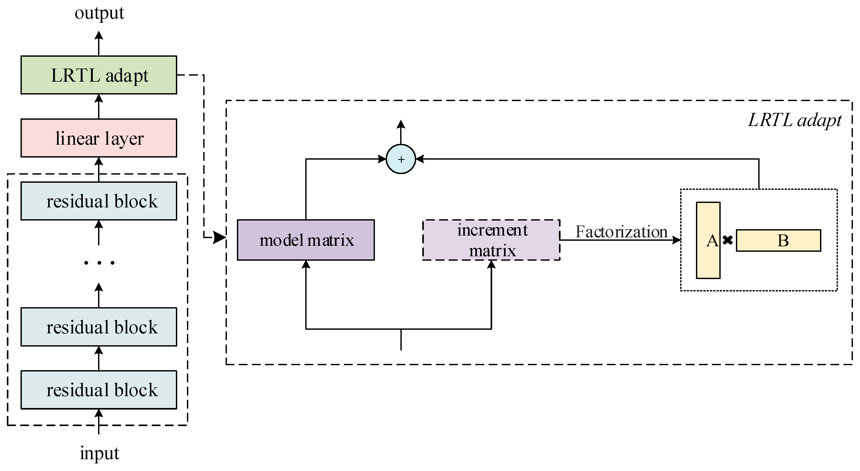
3.4. Low-Rank Attention-Enhanced Temporal Convolutional Transfer Learning (LRTL-AtTCN)

3.4.1. Attention-Enhanced Temporal Convolution Network(AtTCN)

The TCN [16] applies convolutional neural networks to time series tasks. By using causal and dilated convolutions, it captures long-range dependencies efficiently and processes the entire sequence in parallel, unlike RNNs that work sequentially.

TCN typically includes causal convolutions to avoid using future information, dilated convolutions to expand the receptive field, and residual connections to stabilize training and reduce gradient vanishing in deep networks.

Given the input building energy consumption data $\left({\mathit{X}}_{1:t},{\mathit{y}}_{1:t}\right),{\mathit{X}}_{1:t}\in {\mathbb{R}}^{t \times m},{\mathit{y}}_{1:t}\in {\mathbb{R}}^{t \times 1}$, TCN is computed as follows:

$$Z_n^{\left(l\right)}=\sigma \left(\sum _{i=0}^{k-1}{W}_i^{\left(l\right)}\cdot Z_{t-{\left(m+1\right)}_i}^{\left(l-1\right)}+b^{\left(l\right)}\right)+Z_n^{\left(l-1\right)}$$

(5)

where $Z_n^{\left(l\right)}$ denotes the input to the $l_{th}$ layer at the time step $t$. Specifically, when $l=0$, $Z_n^{\left(0\right)}=\left({\mathit{X}}_{1:t},{\mathit{y}}_{1:t}\right)$; $k$ represents the size of the convolution kernel, and $W_i^{\left(l\right)}$ is the weight of the $l_{th}$ convolution kernel in the $l_{th}$ layer. $d_i$ is the dilation factor, and $Z_{t-{(m+1)}_i}^{\left(l-1\right)}$ is the output of the ${\left(l-1\right)}_{th}$ layer at the time step $t={(m+1)}_i$, $b^{\left(l\right)}$ is the bias term for the $l_{th}$ layer, and $\sigma \left(·\right)$ is the activation function.

The attention mechanism [48] enables the model to capture global dependencies by jointly attending to all time steps in the input sequence. This parallel computation improves the modeling of long-range relationships. The multi-head attention mechanism extends this method by performing multiple attention operations in parallel, thereby enhancing the model’s representational capacity. The multi-head attention mechanism can be described as follows:

Given the input building energy consumption data $\left({\mathit{X}}_{1:t},y_{1:t}\right)=\left\{({\mathit{X}}_1,y_1),({\mathit{X}}_2,y_2),\cdots ,({\mathit{X}}_t,y_t)\right\},({\mathit{X}}_i,y_i)\in {\mathbb{R}}^{m+1}$, where $({\mathit{X}}_i,y_i)$ represents the $i_{th}$ input vector, and $m+1$ is the dimension of the input vector. The model uses a multi-head mechanism to compute self-attention scores independently and in parallel. Each attention head, ${head}_i$, is computed as follows:

$$hea{d}_i=Attention\left(Q_i,K_i,V_i\right)$$

(6)

$Q_i,K_i,V_i$ represent the query vector, key vector, and value vector, respectively, where $d_k$ is the dimension of $Q_i,{K_i,V}_i$.

Concatenate the outputs of these heads:

$$MultHead\left(Q,K,V\right)=Concat\left(hea{d}_1,hea{d}_2,\cdots ,hea{d}_n\right)W_O$$

(7)

where $W_O$ is the linear transformation matrix of the output, where $Concat$ indicates concatenating the outputs of all heads along the feature dimension.

In BECP, TCN effectively extracts local features by expanding its receptive field through convolution. However, energy consumption is influenced by complex long-term factors such as seasonal patterns, equipment cycles, and environmental conditions, which exhibit intricate temporal dependencies. Due to its local receptive field, TCN struggles to dynamically focus on such variable factors, limiting its capacity to model long-range dependencies and reducing prediction accuracy.

To address this issue, we propose an innovative Attention-Enhanced Temporal Convolution Network (AtTCN) that integrates the MHA with TCN. As illustrated in Figure 4, this integration enables the model to capture global features and long-term dependencies more effectively. MHA allows dynamic and parallel modeling of temporal relationships, significantly improving the model’s ability to process complex patterns in energy consumption data.

The extraction of local hidden features is achieved through the utilization of multiple convolutional kernels $H_n^{\left(l\right)}$:

$$H_n^{\left(l\right)}=\sum _{i=0}^{k-1}{W}_i^{\left(l\right)}\cdot Z_{n-{(m+1)}_i}^{\left(l-1\right)}+b^{\left(l\right)}$$

(8)

The extracted local hidden features, designated as $H_n^{\left(l\right)}$, are subjected to a linear transformation to generate $Q,K,V$, whose vectors are subsequently computed by MHA. In conjunction with the residual connection structure, the final output, $Z_n^{\left(l\right)}$. AtTCN is computed as follows:

$$Z_n^{\left(l\right)}=\sigma \left(\mathrm{MultiHead}\left(H_t^{\left(l\right)}\cdot \left(W_Q^{\left(l\right)},W_K^{\left(l\right)},W_V^{\left(l\right)}\right)\right)\right)+Z_n^{\left(l-1\right)}$$

(9)

$W_Q^{\left(l\right)},W_K^{\left(l\right)},W_V^{\left(l\right)}$ are the learned matrices that are employed to transform the convolved hidden features $H_n^{\left(l\right)}$ to $Q,K,V$. While retaining TCN’s advantages in local feature extraction and efficiently and flexibly capturing short-term fluctuations, TCN is capable of further capturing long-term trends, thus improving the prediction accuracy and model robustness. With retaining the advantages of TCN in local feature extraction and capturing short-term fluctuations efficiently and flexibly, AtTCN can further capture long-term trends, thereby addressing the complexity of building energy consumption data influenced by multidimensional factors. This enables enhanced prediction accuracy and model robustness.

The AtTCN architecture integrates MHA and TCN to achieve synergy on three levels. First, in terms of feature granularity, TCN captures local patterns through convolution, while MHA refines these features using global context—forming a multi-scale representation akin to a “microscope-telescope” system. Second, for dynamic receptive field adjustment, the attention weights effectively serve as learnable, time-varying dilation factors, allowing the model to adapt its receptive field based on input characteristics. Third, regarding gradient flow, the residual structure creates dual pathways for gradient propagation: preserving local feature stability via TCN and enabling global error correction through the attention branch.

3.4.2. Low-Rank Transfer Learning (LRTL)

Low-rank decomposition [49] is a matrix factorization technique that represents a matrix as the product of lower-rank matrices. It enables dimensionality reduction while preserving key structural information, thus reducing storage and computational costs. This method effectively captures latent features in the data and is widely used in tasks such as data compression and noise reduction.

Given matrix $M\in {\mathbb{R}}^{a\times b}$, the objective of the low-rank decomposition is to identify two matrices, $U\in {\mathbb{R}}^{a\times r}$ and $V\in {\mathbb{R}}^{r\times b}$, such that the matrix A can be approximated as the product of $U$ and $V$:

$$M\approx U\cdot V$$

(10)

where $r$ is a number less than $min\left\{a,b\right\}$.

To address data scarcity challenges in BECP, we propose a transfer learning method with low-rank decomposition (LRTL). This method introduces an incremental matrix derived from pre-trained source model weights, enabling rapid adaptation to new buildings by fine-tuning target features. Compared to traditional methods, LRTL reduces parameter dimensionality while preserving essential source domain features, which alleviates overfitting and improves generalization. Moreover, low-rank decomposition mitigates domain differences, ensuring stable and accurate predictions even with limited data.

Given the pre-trained model weight matrix $W\in {\mathbb{R}}^{a\times b}$, we introduce an incremental matrix $W^0\in {\mathbb{R}}^{a\times b}$ for weight updates:

$$W^{\prime }=W+W^0$$

(11)

$W^{\prime }$ is the transferred model weight matrix, where $d$ represents the input dimension, and k is the output dimension.

Directly optimizing $W^0$ in such a high-dimensional space is computationally expensive and prone to overfitting. To mitigate these issues, we apply a low-rank decomposition to $W^0$, expressing it as the product of two smaller matrices $A\in {\mathbb{R}}^{a\times r}$ and $B\in {\mathbb{R}}^{r\times b}$, where $r$ is a rank that is much smaller than $\min \left\{a,b\right\}$. This decomposition reduces the complexity of the update by capturing the most significant variations in a lower-dimensional subspace. Intuitively, this is equivalent to representing a large, complex transformation as two simpler, consecutive transformations.

Accordingly, the updated weight matrix becomes

$$W^{\prime }=W+BA$$

(12)

Given a source building domain model $f^S:{(\mathit{X}}_{1:t^S}^S,{\mathit{y}}_{1:t^S}^S)\to {(\mathit{X}}_{t^S+1:t^S+\Omega }^S,{\mathit{y}}_{t^S+1:t^S+\Omega }^S)$, the objective is to learn a target building domain model $f^T:{(\mathit{X}}_{1:t^T}^T,{\mathit{y}}_{1:t^T}^T)\to {(\mathit{X}}_{t^T+1:t^T+\Omega }^T,{\mathit{y}}_{t^T+1:t^T+\Omega }^T)$, where $f^T$ minimizes the prediction error in the target building domain by effectively utilizing the information from the source building domain. Low-Rank Transfer Learning is computed as follows:

$$f^T=\underset{f^T}{argmin}\left(E_{{(\mathit{X}}_{1:t^T}^T,{\mathit{y}}_{1:t^T}^T)~D^T}\left(\mathcal{L}\left(f^T;W+BA\right)\right)+\lambda E_{{(\mathit{X}}_{1:t^S}^S,{\mathit{y}}_{1:t^S}^S)~D^S}\left(\mathcal{L}\left(f^S;W\right)\right)\right)$$

(13)

where $\mathcal{L}\left(\cdot \right)$ denotes the loss function, and $\lambda$ is the hyperparameter that balances the losses between the source building domain and the target building domain.

As illustrated in Figure 5, we freeze the model’s hidden feature extraction layers and fine-tune only the final prediction layer. This preserves the model’s ability to capture local and global features while adapting the prediction layer to the target domain. This method reduces training costs and mitigates overfitting, improving transfer learning efficiency and generalization. Experimental results show significant performance gains in predicting building energy consumption with varying feature distributions.

LRTL reduces the number of parameters during model optimization while preserving essential features from the source building’s energy consumption task. This enables rapid adaptation to the target building’s characteristics, improving transfer efficiency. The low-rank structure enhances robustness and mitigates overfitting, maintaining high prediction accuracy even with limited data.

3.4.3. Algorithm

Algorithm 1 systematically details the LRTL-AtTCN for BECP, structured into two stages: the source domain training stage and the transfer learning stage. In the initial stage, the AtTCN model is trained on the source building data, which captures localized temporal features through convolutional layers and enhances global hidden features using multi-head attention mechanism with residual connections. In the subsequent Transfer Learning Stage, the pretrained AtTCN model is adapted to the target building data using the Low-Rank Transfer Learning (LRTL) technique. This adaptation refines the model weights to account for domain-specific variations, employing low-rank decomposition to facilitate knowledge transfer.

Algorithm 1 LRTL-AtTCN method for energy consumption prediction
Input: Source building energy consumption data ${(\mathit{X}}_{1:t^S}^S,{\mathit{y}}_{1:t^S}^S)\in {\mathbb{R}}^{t\mathrm{ }\times \mathrm{ }m+1}\mathrm{ }$ and target energy consumption data ${(\mathit{X}}_{1:t^T}^T,{\mathit{y}}_{1:t^T}^T)\in {\mathbb{R}}^{t\mathrm{ }\times \mathrm{ }m+1}\mathrm{ }$, where $\mathit{X}$ is external features, y is building energy consumption data, $n$ is the number of the time steps, and $m$ is the number of features, the last column is the target variable;
Output: predicted values for the target variable.
1:	Source Domain Training Stage
2:	Initialize AtTCN model;
3:	for episode = 1 to EPISODES do
4:	for each layer $l$ do
5:	$H_n^{\left(l\right)}={\sum }_{i=0}^{k-1}{W}_i^{\left(l\right)}·Z_{n-{(m+1)}_i}^{\left(l-1\right)}+b^{\left(l\right)};$
6:	$Z_n^{\left(l\right)}=\mathsf{\sigma }\left(\mathrm{MultiHead}\left(H_t^{\left(l\right)}\cdot \left(W_Q^{\left(l\right)},W_K^{\left(l\right)},W_V^{\left(l\right)}\right)\right)\right)+Z_n^{\left(l-1\right)}$;
7:	end for
8:	$output={W·Z}_n^{\left(l\right)}+b$;
9:	Loss computation: $\mathcal{L}\left(\theta \right)=MSE(output,true\_y)$;
10:	Update AtTCN using: $\theta \leftarrow \theta -{\eta \nabla }_{\theta }\mathcal{L}$;
11:	end for
12:	Save AtTCN model;
13:
14:	Transfer Learning Stage
15:	Initialize LRTL model and load AtTCN model;
16:	for episode = 1 to EPISODES do
17:	compute the forward pass using the model weights ($W+BA$);
18:	loss computation: $\mathcal{L}\left(\theta \right)=MSE(output,true\_y)$;
19:	Update $B$ using: $B\leftarrow B-\eta \nabla B\mathcal{L}$;
20:	Update $A$ using: $A\leftarrow A-\eta \nabla A\mathcal{L}$;
21:	end for
22:	Save transferred model

4. Results

4.1. Experiments Setting

This section presents a comprehensive evaluation of LRTL-AtTCN. In the experiment, the source domain data consists of weather and energy consumption data from a building collected between 2016 and 2017, with a data sampling interval of one hour. To simulate a scenario with limited data availability, we selected data from another similar building over three different time spans (one month, two weeks, and one week) as the data source for the target domain. The features utilized in the experimental study were determined through Granger causality analysis. To facilitate comparison with the performance of the subsequent transfer model, the energy consumption data of different buildings are normalized uniformly.

The experimental analysis is conducted from three aspects: (1) Method performance: We evaluate the performance of the AtTCN model in the source domain, and compare it with XGBoost [11], LSTM [13], CNN-LSTM [50], TCN [16], and iTransformer [51]. Then, we analyze LRTL’s transfer performance in the target domain, and compare it with some state-of-the-art transfer learning methods; (2) Method details analysis: A detailed examination of the LRTL-AtTCN model is performed from two aspects, including feature combination and rank setting; (3) Ablation analysis: To comprehensively analyze the impact of different components on the overall performance of the LRTL-AtTCN, we conduct a comparative evaluation with several widely adopted models, including LSTM, CNN-LSTM, TCN, and iTransformer. To gain deeper insights into the integration of TCN and the attention mechanism, we conduct experimental comparisons by varying the placement of the attention layers, aiming to further investigate the influence of the attention mechanism in LRTL-AtTCN.

4.2. Evaluation Metrics

To comprehensively evaluate the prediction performance in the source building domain and the transfer performance in the target building domain, a series of key metrics were employed, including the mean absolute error, MAE, measuring the average magnitude of errors, mean square error, MSE, penalizing larger errors more heavily, and coefficient of determination, R², indicating how well the model captures the variance, which provides insight into its prediction performance:

$$MAE={\displaystyle \frac{1}{N}}\sum _{i=1}^N\left|y_i-\widehat{y_i}\right|$$

(14)

$$MSE={\displaystyle \frac{1}{N}}\sum _{i=1}^N{\left(y_i-\widehat{y_i}\right)}^2$$

(15)

$$MAPE={\displaystyle \frac{1}{n}}\sum _{i=1}^n\left|{\displaystyle \frac{y_i-\widehat{y_i}}{y_i}}\right|\times 100\%$$

(16)

$$R^2=1-{\displaystyle \frac{{\sum }_{i=1}^N{\left(y_i-\widehat{y_i}\right)}^2}{{\sum }_{i=1}^N{\left(y_i-\overline{y}\right)}^2}}$$

(17)

where $y_i$ denotes the true value at the time step $i$, $\widehat{y_{\mathrm{i}}}$ denotes the predicted value at the same the time step, $N$ denotes the total number of samples, and $\overline{y}$ denotes the mean actual value across all the time steps.

4.3. Results and Analysis

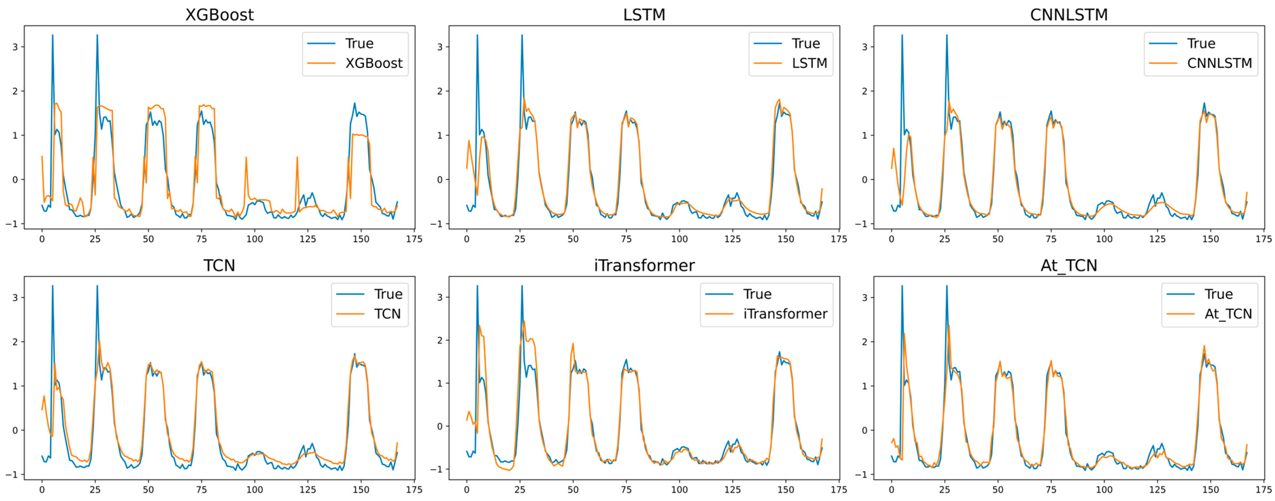
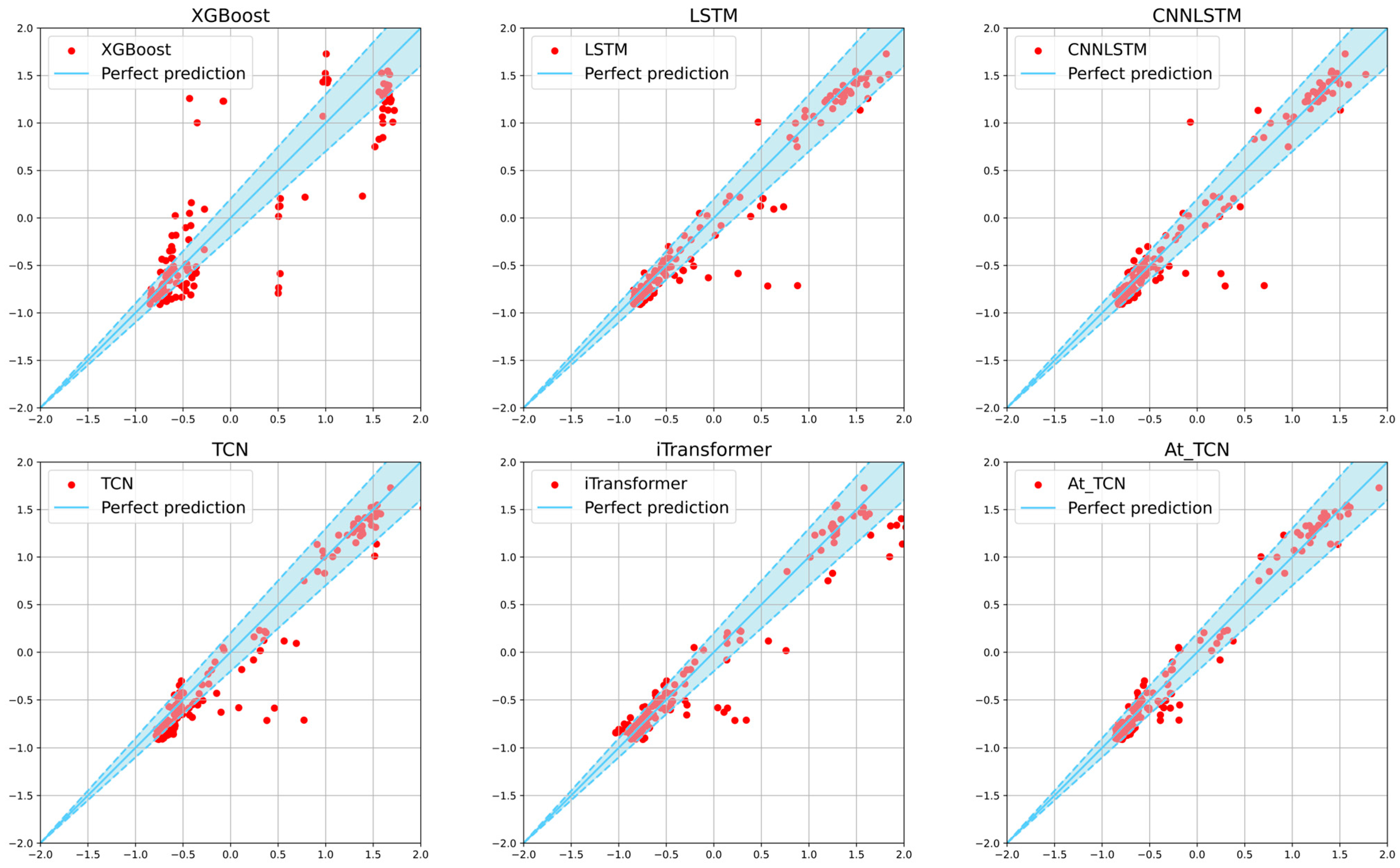
4.3.1. Method Performance Comparison

To evaluate the prediction performance of LRTL-AtTCN in the source domain, we compared AtTCN with other traditional and state-of-the-art methods. The results, reported as mean values with 95% confidence intervals, are presented in

Table 3. Source Domain Performance of Different Methods (Mean ± 95% CI).

Method	$\mathbf{M}\mathbf{A}\mathbf{E}$	$\mathbf{M}\mathbf{S}\mathbf{E}$	$\mathbf{M}\mathbf{A}\mathbf{P}\mathbf{E}$	${\mathbf{R}}^2$
Xgboost [11]	0.2092 ± 0.0164	0.1161 ± 0.0234	111.93% ± 21.45%	0.8497 ± 0.0303
LSTM [13]	0.1072 ± 0.0041	0.0348 ± 0.0013	36.26% ± 1.29%	0.9459 ± 0.0017
CNNLSTM [50]	0.1010 ± 0.0065	0.0321 ± 0.0020	41.72% ± 3.88%	0.9509 ± 0.0026
TCN [16]	0.1046 ± 0.0190	0.0278 ± 0.0044	51.46% ± 5.96%	0.9611 ± 0.0056
iTransformer [51]	0.0887 ± 0.0023	0.0248 ± 0.0007	35.83% ± 2.65%	0.9674 ± 0.0009
AtTCN (Ours)	0.0830 ± 0.0026	0.0234 ± 0.0005	35.21% ± 2.01%	0.9696 ± 0.0007

. Results shows that AtTCN outperforms XGBoost significantly, reducing MAE from 0.2092 to 0.0830, MSE from 0.1161 to 0.0234, MAPE from 143.69% to 35.21%, and increasing R² from 0.8497 to 0.9674. Compared with LSTM, CNN-LSTM, and TCN, AtTCN achieves lower MAE, MSE, and MAPE, indicating superior prediction accuracy. Against TCN, AtTCN’s attention mechanism enables it to capture latent features better, reducing MAE and MSE by 0.0216 and 0.0044, respectively, while improving R² by 0.0063 and MAPE by 16.25%. Notably, AtTCN surpasses iTransformer in MAE, MSE, and MAPE with an equivalent R² of 0.9674, demonstrating its high efficiency in a streamlined structure. Thus, AtTCN exhibits robust prediction performance with lower error rates and better model fitness in the source domain.

Figure 6 illustrates the prediction results of different methods, where the horizontal axis represents the time step, the vertical axis represents normalized energy consumption, the blue line represents the actual normalized energy consumption data, and the yellow line denotes the method’s predictions without inverse normalization in each subplot.

Compared to the traditional method XGBoost, AtTCN model demonstrates a much closer fit to the true values, particularly in capturing peaks and valleys, where it exhibits significantly higher accuracy, while XGBoost shows larger deviations from the true values, especially at the extremes, resulting in noticeable errors. This indicates that AtTCN possesses a stronger prediction performance for complex time series data. Compared to LSTM and CNNLSTM, three methods all show relatively small deviations from the true values, especially in regions with minimal fluctuations. However, in specific local areas, such as the peaks and valley, AtTCN’s predictions align more closely with the true values, resulting in smaller prediction errors, which suggests AtTCN has better prediction performance. In comparison with TCN, AtTCN’s prediction curve is smoother and aligns more closely with the true values, especially in the peak and valley areas. The addition of the attention mechanism allows AtTCN to capture global temporal dependencies dynamically and more effectively, leading to higher precision, particularly at critical data points. Moreover, AtTCN and iTransformer exhibit highly similar prediction curves, both showing a strong fit in the peaks and valleys, with their curves almost overlapping the true values. Therefore, AtTCN consistently outperforms other models in various comparisons. In complex time series prediction tasks, AtTCN not only captures the overall trends of the data but also leverages the attention mechanism to handle local fluctuations with greater precision.

Figure 7 also provides insights into the performance of various methods from a different perspective. The horizontal axis represents normalized actual values, while the vertical axis denotes normalized predicted values. The solid blue line indicates perfect alignment between predicted and actual values, the blue dashed lines represent a ±20% margin of error, and the shaded area defines an acceptance interval (AI) where the prediction error is within 20%. A similar AI-based visualization was also employed by Li et al. [52], supporting the validity of this method. Compared to the traditional method XGBoost, AtTCN demonstrates more stable predictions, while XGBoost exhibits significant deviations from the true values, particularly showing larger fluctuations and errors in areas where predictions diverge. Compared to LSTM and CNNLSTM, AtTCN provides slightly better performance in capturing local details, especially at extreme points and regions with high variability. When compared to TCN, AtTCN’s prediction points are smoother and more tightly clustered around the ideal prediction line, particularly in peak and valley regions, where the attention mechanism significantly enhances the model’s ability to capture both global and local dependencies dynamically, further improving prediction performance. Moreover, compared to iTransformer, both models show a strong fit near the “perfect prediction” line, with nearly identical performance on complex time series data. Therefore, AtTCN delivers superior results in terms of prediction performance and stability, particularly in complex time series prediction tasks.

We evaluated the transfer performance of LRTL-AtTCN in the target domain, using the performance of AtTCN trained directly in the target domain as a benchmark. Subsequently, we compared the performance of fine-tuned AtTCN, LRTL-AtTCN, and other transfer learning methods.

Table 4. Transfer Performance of Different Methods Across Various Time Series (Mean ± 95% CI).

Time Series	Method	$\mathbf{M}\mathbf{A}\mathbf{E}$	$\mathbf{M}\mathbf{S}\mathbf{E}$	$\mathbf{M}\mathbf{A}\mathbf{P}\mathbf{E}$	${\mathbf{R}}^2$
1 Week	AtTCN(baseline)	1.2116 ± 0.2805	1.7144 ± 0.6034	2673% ± 2474%	-
	fine-tuned AtTCN	0.9848 ± 0.2535	1.2330 ± 0.4055	2077% ± 2040%	-
	aRATL [40]	0.8342 ± 0.2992	0.8556 ± 0.4419	449.40% ± 276.39%	-
	DCORAL [41]	0.5852 ± 0.3015	0.5060 ± 0.3513	63.54% ± 32.54%	-
	Fine-Grained RNN&TL [42]	0.2345 ± 0.0010	0.0551 ± 0.0005	25.49% ± 0.11%	-
	Freeze-LSTM [43]	0.0618 ± 0.0004	0.0618 ± 0.0004	27.01% ± 0.10%	-
	LRTL-AtTCN(Ours)	0.1064 ± 0.0280	0.0150 ± 0.0168	16.10% ± 0.86%	-
2 Weeks	AtTCN(baseline)	0.3619 ± 0.1830	0.3236 ± 0.2086	702.31% ± 980.99%	-
	fine-tuned AtTCN	0.2529 ± 0.1565	0.1306 ± 0.1915	392.01% ± 401.24%	0.6642 ± 0.2570
	aRATL [40]	0.2860 ± 0.0292	0.0898 ± 0.0157	293.13% ± 160.11%	0.5435 ± 0.0698
	DCORAL [41]	0.4146 ± 0.1220	0.2989 ± 0.1393	277.04% ± 117.03%	0.3557 ± 0.4040
	Fine-Grained RNN&TL [42]	0.3114 ± 0.0001	0.1337 ± 0.0001	275.87% ± 0.24%	0.3924 ± 0.0005
	Freeze-LSTM [43]	0.2994 ± 0.0001	0.1146 ± 0.0001	284.04% ± 0.24%	0.0813 ± 0.0002
	LRTL-AtTCN(Ours)	0.1859 ± 0.0113	0.0533 ± 0.0035	155.10% ± 4.95%	0.8628 ± 0.0155
1 Month	AtTCN(baseline)	0.3059 ± 0.2190	0.1810 ± 0.4073	132.95% ± 132.85%	0.8188 ± 0.2058
	fine-tuned AtTCN	0.2742 ± 0.2075	0.1353 ± 0.2033	86.85% ± 75.27%	0.8763 ± 0.2101
	aRATL [40]	0.2408 ± 0.0294	0.1062 ± 0.026	67.51% ± 29.06%	0.9038 ± 0.0316
	DCORAL [41]	0.2401 ± 0.0073	0.1030 ± 0.0041	66.53% ± 5.95%	0.9018 ± 0.0029
	Fine-Grained RNN&TL [42]	0.3041 ± 0.0001	0.1332 ± 0.0001	50.57% ± 0.01%	0.8769 ± 0.0001
	Freeze-LSTM [43]	0.3594 ± 0.0001	0.1956 ± 0.0001	66.13% ± 0.01%	0.7983 ± 0.0002
	LRTL-AtTCN(Ours)	0.2251 ± 0.0124	0.0911 ± 0.085	50.57% ± 3.75%	0.9286 ± 0.0157

summarizes the transfer performance of different methods across various time series under limited data conditions. Due to the small sample size in the target building domain, R² values for one-week predictions were omitted, and results are reported as means with 95% confidence intervals. Compared with the fine-tuned AtTCN, LRTL-AtTCN consistently achieves lower MAE, MSE, and MAPE across all forecasting horizons, indicating its superior capacity to capture temporal patterns with greater accuracy and stability. In short-term forecasting, LRTL-AtTCN outperforms aRATL by a considerable margin, particularly in MAPE and MAE, suggesting enhanced precision in low-data regimes. While aRATL improves over longer horizons, LRTL-AtTCN maintains stronger data fitting and robustness. Compared with DCORAL, LRTL-AtTCN exhibits markedly reduced MAE and MSE in both one- and two-week settings, especially excelling in MSE reduction. Moreover, DCORAL requires domain alignment steps, incurring additional transfer costs. Fine-Grained RNN with transfer learning and Freeze-LSTM demonstrate competitive performance in one-week predictions, with low errors and narrow confidence intervals, but their effectiveness diminishes at longer horizons. In contrast, LRTL-AtTCN delivers the most balanced and consistent performance across all time spans.

In summary, LRTL-AtTCN excels in scenarios with limited target data, outperforming state-of-the-art baselines by effectively reducing redundant parameters via low-rank decomposition. This results in lower adaptation cost and better generalization across various prediction intervals.

Figure 8 illustrates the prediction results of different transfer learning methods, where the horizontal axis represents the time step, the vertical axis represents normalized energy consumption, the blue line represents the actual normalized energy consumption data, and the yellow line denotes the method’s predictions without inverse normalization in each subplot. Compared to finetune and aRATL, LRTL consistently achieves better overall fitting performance. Although finetune captures the general trend of energy consumption, there is a significant deviation between the predicted and actual values. aRATL demonstrates satisfactory performance in fitting intermediate values; however, its ability to fit peak and trough values is relatively weak. In comparison to DCORAL, LRTL performs similarly in terms of overall fitting quality, but outperforms DCORAL in fitting trough values, while its fitting of peak values is slightly inferior to that of DCORAL. The Freeze LSTM method exhibits a moderate ability to capture both peak and trough values but suffers from noticeable deviations in certain intermediate periods, indicating instability in its predictions. On the other hand, the Fine-Grained RNN with Transfer Learning achieves a more stable fitting of general trends, with relatively accurate intermediate values. However, like aRATL, it struggles with accurately predicting extreme peaks and troughs. Overall, LRTL maintains its superior performance by consistently demonstrating better fitting of both intermediate and extreme values, reinforcing its robustness and adaptability across different time steps.

Figure 9 illustrates the absolute errors of various transfer learning methods: finetune, aRATL, DCORAL, Freeze LSTM, Fine-Grained RNN with TL, and LRTL. The horizontal axis represents the models, while the vertical axis shows the absolute error values. Each boxplot depicts the distribution of errors for the respective method, including the interquartile range (IQR), median (orange line), and range (whiskers). Among all methods, LRTL demonstrates the lowest overall error distribution, with a smaller interquartile range (IQR) and a lower median absolute error compared to the other methods. The compactness of the box for LRTL indicates that its predictions are consistently closer to the true values, reflecting higher accuracy and stability across various time steps. Finetune and aRATL have much larger error distributions, with both higher medians and significantly wider IQRs, implying that these methods struggle with achieving consistent accuracy, leading to higher variability in their predictions. While DCORAL and Freeze LSTM show reduced error variability compared to finetune and aRATL, their medians remain higher than that of LRTL, indicating inferior overall prediction accuracy. Fine-Grained RNN with TL achieves a comparable error distribution to LRTL but has a slightly larger median and IQR, suggesting that it performs well but still falls short of LRTL’s precision. Both finetune and aRATL exhibit larger error ranges and potential outliers, further demonstrating their inconsistency. In contrast, LRTL maintains a tight error range, highlighting its robustness and reliability across different conditions. The boxplot effectively demonstrates that LRTL outperforms all other methods in terms of accuracy and stability. Its minimal error distribution, low median, and compact IQR underline its superior ability to generalize and adapt, making it the most reliable method for transfer learning in this context.

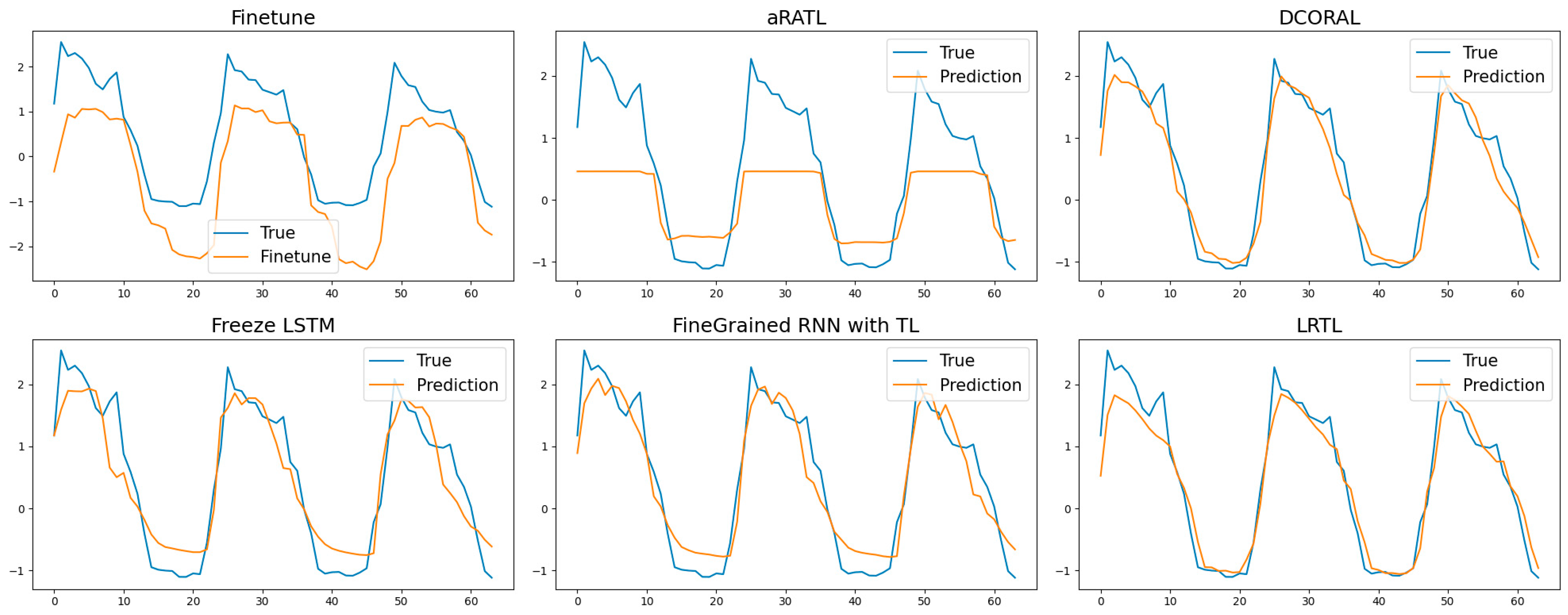
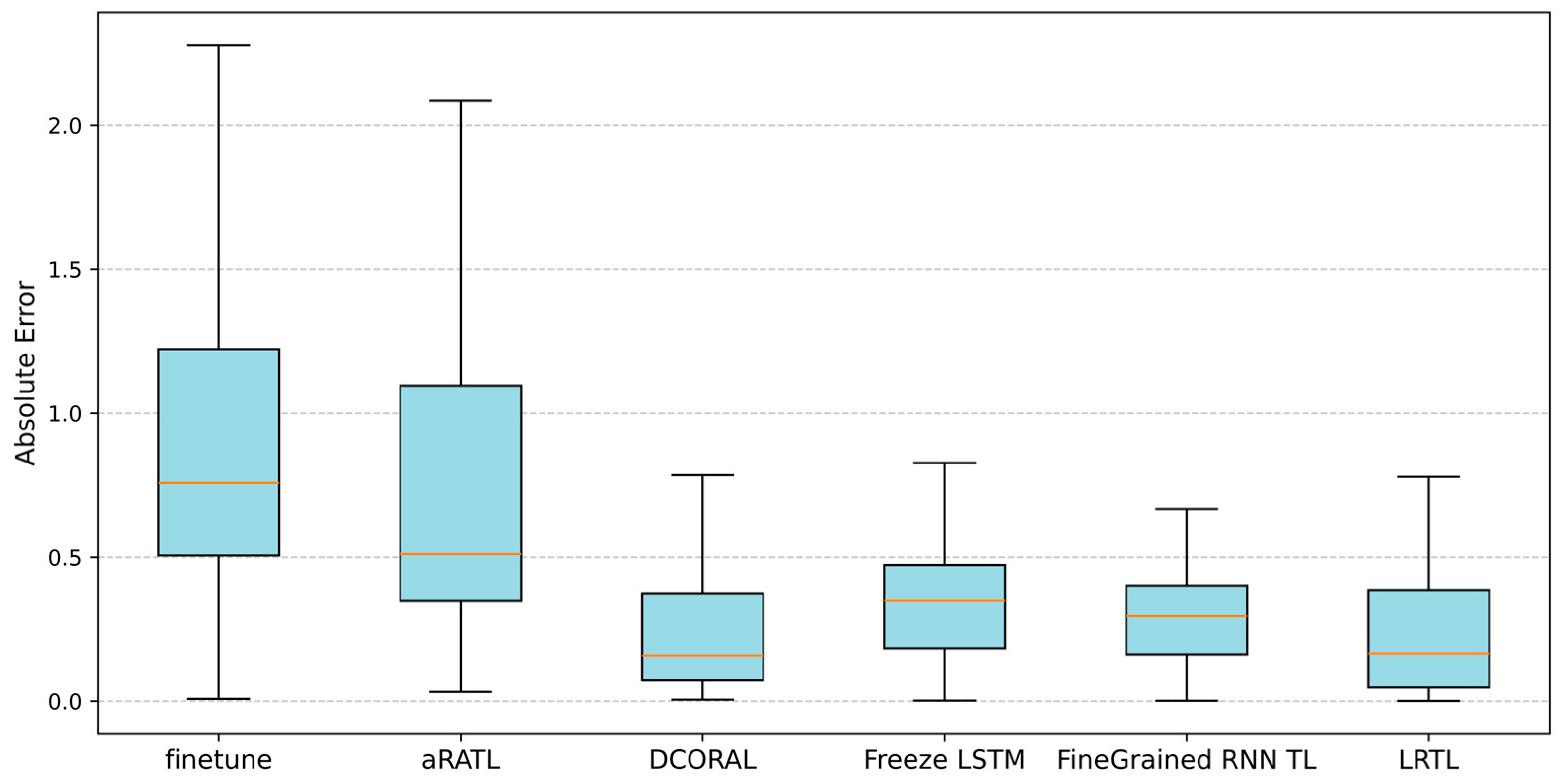
4.3.2. Method Details Exploration

We analyze the impact of different feature combinations on the LRTL-AtTCN’s overall performance, and feature combination and results of the experiment are shown in

Table 5. Feature Combination Impact on LRTL-AtTCN Transfer Performance (1-Month).

ID	Feature Combination	$\mathbf{M}\mathbf{A}\mathbf{E}$	$\mathbf{M}\mathbf{S}\mathbf{E}$	$\mathbf{M}\mathbf{A}\mathbf{P}\mathbf{E}$	${\mathbf{R}}^2$
F1	energy features	0.3737 ± 0.0050	0.2696 ± 0.0056	183.25% ± 8.20%	0.7805 ± 0.0059
F2	energy features + weather feature	0.3059 ± 0.0076	0.1263 ± 0.0079	161.22% ± 5.21%	0.8783 ± 0.0145
F3	energy features + timestamp features	0.3402 ± 0.0009	0.2150 ± 0.0008	102.88% ± 1.82%	0.8227 ± 0.0053
F4	energy features + weather feature + timestamp features	0.2770 ± 0.0031	0.1012 ± 0.0027	54.81% ± 1.30%	0.9111 ± 0.0050
F5	Granger-selected feature	0.2251 ± 0.0124	0.0911 ± 0.085	50.57% ± 3.75%	0.9286 ± 0.0157

. The inclusion of weather and timestamp features consistently improves model performance across all evaluation metrics, including MAE, MSE, MAPE, and R². A comparison between F2 and F3 reveals that weather features contribute more substantially to performance enhancement than timestamp features, as evidenced by the lower MAE and MAPE values in F2. Interestingly, although F4 includes more features than F5, F5—constructed based on the results of Granger causality analysis—achieves the best overall performance. The Granger analysis reveals a strong causal relationship between weather factors and energy consumption, whereas only two timestamp-related features (“hour of the day” and “holiday status”) exhibit a meaningful causal link. The inclusion of non-causally related timestamp features in F4 appears to introduce noise, slightly impairing performance compared to the more selective F5. These results demonstrate that Granger causality analysis serves as an effective feature selection method, helping to refine the input space and improve model accuracy across all four metrics, particularly in reducing MAPE.

Table 6. LRTL-AtTCN Parameters and Transfer Parameters Metrics.

Rank	$\mathbf{Parameter}\mathbf{Count}$	$\mathbf{Transfer}\mathbf{Parameter}\mathbf{Count}$	$\mathbf{Parameters}\mathbf{Reduction}\mathbf{Ratio}$
4	16,681	260	0.9844
8	16,689	520	0.9688
16	16,705	1040	0.9377
32	16,737	2080	0.8757
64	16,801	4160	0.7524

presents the parameters and transfer metrics for the LRTL-AtTCN method across different ranks. It is evident that the number of fine-tuning parameters during the transfer stage of LRTL-AtTCN has been significantly reduced. In conjunction with the results depicted in

Table 7. Different Rank Setting on LRTL-AtTCN Transfer Performance (1-Month).

Rank Setting	$\mathbf{M}\mathbf{A}\mathbf{E}$	$\mathbf{M}\mathbf{S}\mathbf{E}$	$\mathbf{M}\mathbf{A}\mathbf{P}\mathbf{E}$	${\mathbf{R}}^2$
4	0.2251 ± 0.0124	0.0911 ± 0.085	50.57% ± 3.75%	0.9286 ± 0.0157
8	0.2919 ± 0.0058	0.1432 ± 0.0040	103.39% ± 2.34%	0.8638 ± 0.0069
16	0.2934 ± 0.0111	0.1439 ± 0.0078	123.57% ± 4.71%	0.8624 ± 0.0135
32	0.2955 ± 0.0283	0.1459 ± 0.0210	154.81% ± 5.30%	0.8576 ± 0.0399
64	0.3064 ± 0.0158	0.1587 ± 0.0113	168.20% ± 9.50%	0.8333 ± 0.0218

, the focus is on evaluating the impact of different rank settings (rank = 4, rank = 8, rank = 16, rank = 32, and rank = 64) on the method’s performance, where MAE, MSE, and R² values are represented using blue, green, and orange bars, respectively, with the R² values additionally connected by a dashed trend line for clarity.

Table 6 and Table 7 illustrate the impact of different rank settings on model parameterization and transfer performance of LRTL-AtTCN. As shown in Table 6, increasing the rank results in a higher number of transfer parameters, thereby reducing the parameter reduction ratio, and increasing model complexity during the transfer stage. However, as observed in Table 7, this increase in model complexity does not lead to improved performance; on the contrary, performance metrics such as MAE, MSE, MAPE, and R² deteriorate as the rank grows. We speculate that larger ranks introduce more trainable parameters, which increases the risk of overfitting on the limited target domain data. This overfitting may cause the model to rely excessively on source-domain-specific features, hindering its generalization ability and, thus, reducing transfer effectiveness.

In contrast, lower-rank configurations (e.g., rank = 4) achieve better overall performance while significantly reducing the number of transfer parameters—achieving a parameter reduction ratio as high as 0.9844. These results suggest that low-rank transfer not only helps control model size and computational costs but also enhances generalization by mitigating overfitting. Therefore, selecting an appropriate rank is essential to balance model complexity and transfer performance, especially in data-scarce scenarios.

4.3.3. Ablation Analysis

Table 8. Ablation Study on Transfer Strategies for Time Series Prediction.

Time Series	Transfer Strategies	$\mathbf{M}\mathbf{A}\mathbf{E}$	$\mathbf{M}\mathbf{S}\mathbf{E}$	$\mathbf{M}\mathbf{A}\mathbf{P}\mathbf{E}$	${\mathbf{R}}^2$
1 Week	direct training	1.2116 ± 0.2805	1.7144 ± 0.6034	2673% ± 2474%	-
	unadapted	0.1668	0.0278		-
	fine-tuned	0.9848 ± 0.2535	1.2330 ± 0.4055	2077% ± 2040%	-
	unifying training	0.2941 ± 0.0145	0.0869 ± 0.0085	47.07% ± 3.45%	-
	LRTL	0.1064 ± 0.0280	0.0150 ± 0.0168	16.10% ± 0.86%	-
2 Weeks	direct training	0.3619 ± 0.1830	0.3236 ± 0.2086	702.31% ± 980.99%	-
	unadapted	0.3043	0.1193		0.5912
	fine-tuned	0.2529 ± 0.1565	0.1306 ± 0.1915	392.01% ± 401.24%	0.6642 ± 0.2570
	unifying training	0.2505 ± 0.0220	0.0851 ± 0.0154	172.04% ± 60.20%	0.4594 ± 0.1512
	LRTL	0.1859 ± 0.0113	0.0533 ± 0.0035	155.10% ± 4.95%	0.8628 ± 0.0155
1 Month	direct training	0.3059 ± 0.2190	0.1810 ± 0.4073	132.95% ± 132.85%	0.8188 ± 0.2058
	unadapted	0.2903	0.1285		0.8772
	fine-tuned	0.2742 ± 0.2075	0.1353± 0.2033	86.85% ± 75.27%	0.8763 ± 0.2101
	unifying training	0.3487 ± 0.0143	0.1656 ± 0.0143	143.78% ± 31.13%	0.8600 ± 0.0110
	LRTL	0.2251 ± 0.0124	0.0911 ± 0.085	50.57% ± 3.75%	0.9286 ± 0.0157

presents an ablation study that compares various transfer strategies for time series prediction across different horizons. Among them, direct training, which uses only limited target data, performs worst due to its lack of transfer mechanisms and high susceptibility to overfitting, especially under data-scarce conditions. It is also not repeated across runs, so statistical measures are not reported. Similarly, the unadapted strategy, applying a source-trained model directly to the target domain, suffers from domain misalignment and lacks generalization, with no statistical variability reported due to its deterministic inference. The fine-tuned approach improves performance by adjusting the model with target data, partially reducing domain gaps, but it still faces overfitting risks due to limited data. The unified training method combines source and target data, increasing data volume but struggling with domain shifts. In contrast, the proposed LRTL method consistently outperforms others by enforcing a low-rank constraint on transfer layers. This reduces parameters, retains source knowledge, and enhances adaptation. LRTL is especially effective for longer horizons, achieving an R² of 0.9286 and the lowest MAE and MAPE in the 1-month task, confirming the robustness of low-rank transfer under limited data conditions.

Table 9. Source Domain Model Impact on LRTL-AtTCN Transfer Performance (1-Month).

Source Domain Combination	$\mathbf{M}\mathbf{A}\mathbf{E}$	$\mathbf{M}\mathbf{S}\mathbf{E}$	$\mathbf{M}\mathbf{A}\mathbf{P}\mathbf{E}$	${\mathbf{R}}^2$
LRTL-LSTM	0.3888 ± 0.0022	0.2063 ± 0.0026	121.40% ± 2.16%	0.8060 ± 0.0078
LRTL-CNNLSTM	0.3342 ± 0.0002	0.1581 ± 0.0005	109.08% ± 0.78%	0.8645 ± 0.0021
LRTL-TCN	0.2923 ± 0.0005	0.1120 ± 0.0010	374.04% ± 4.34%	0.9000 ± 0.0030
LRTL-iTransformer	0.2746 ± 0.0020	0.1171 ± 0.0015	80.36% ± 0.77%	0.9018 ± 0.0028
LRTL-AtTCN	0.2251 ± 0.0124	0.0911 ± 0.085	50.57% ± 3.75%	0.9286 ± 0.0157

illustrates the impact of different source domain models on the transfer performance of LRTL-AtTCN over a one-month prediction horizon. Compared with LRTL-LSTM and LRTL-CNNLSTM, LRTL-AtTCN achieves notably better predictive accuracy, indicating that the attention-enhanced TCN structure is more effective in capturing transferable temporal patterns. During the transfer process, the attention mechanism in LRTL-AtTCN enables dynamic focus on salient features from the source domain, which facilitates more robust adaptation and mitigates performance degradation. When compared to LRTL-TCN, LRTL-AtTCN consistently maintains superior performance, suggesting that the integration of attention further enhances the temporal representation capability beyond conventional convolutional architectures. Additionally, although LRTL-iTransformer also incorporates attention, LRTL-AtTCN demonstrates greater adaptability and robustness, due to its hybrid design that leverages both temporal convolution and attention mechanisms. Consequently, AtTCN exhibits exceptional performance in LRTL. The integration of the attention mechanism not only enhances the model’s prediction accuracy but also strengthens its adaptability during the transfer process, allowing for more effective migration of features learned in the source domain to the target domain.

We conducted a comparative analysis of the impact of different sequences of convolutional and attention layers on the performance of the LRTL-AtTCN, which is shown in

Table 10. Layer Arrangements Impact on LRTL-AtTCN Transfer Performance (1-Month).

Layer Arrangements	$\mathbf{M}\mathbf{A}\mathbf{E}$	$\mathbf{M}\mathbf{S}\mathbf{E}$	$\mathbf{M}\mathbf{A}\mathbf{P}\mathbf{E}$	${\mathbf{R}}^2$
attention + conv1 + conv2	0.2779 ± 0.0001	0.1076 ± 0.0002	45.25% ± 0.19%	0.9117 ± 0.0007
conv1 + attention + conv2	0.2690 ± 0.0004	0.1028 ± 0.0005	293.30% ± 1.51%	0.9167 ± 0.0012
conv1 + conv2 + attention	0.2251 ± 0.0124	0.0911 ± 0.085	50.57% ± 3.75%	0.9286 ± 0.0157

. The results demonstrate that the sequence of these layers exerts a substantial influence on model performance. Notably, the configuration of “conv1 + conv2 + attention” yields the best performance in terms of MAE, MSE, and R². This suggests that performing convolutional operations prior to attention enables more effective feature extraction, thereby allowing the attention mechanism to better focus on critical temporal patterns. Moreover, this configuration also achieves the lowest MAPE, indicating enhanced robustness and relative accuracy across varying scales. These findings highlight the crucial role of architectural design in improving the model’s capability to generalize and accurately predict energy consumption patterns.

4.3.4. Discussion

In this paper, we propose LRTL-AtTCN, a novel transfer learning method addressing limited data availability in BECP. By integrating the attention mechanism with TCN, the method effectively captures both local and global hidden features. Experimental results show that AtTCN achieves prediction accuracy comparable to state-of-the-art models while maintaining superior stability, validating the effectiveness of combining attention with TCN. In the transfer stage, low-rank decomposition is introduced, significantly reducing model complexity without compromising transfer performance. We attribute this improvement to the reduction in model parameters and redundancy. Additionally, we thoroughly evaluate the method by analyzing feature combinations, rank settings, network components, and layer sequences. These findings confirm that LRTL-AtTCN effectively tackles the data scarcity challenge in BECP.

5. Conclusions

This paper proposes LRTL-AtTCN, a transfer learning method that integrates low-rank decomposition with TCN and incorporates attention mechanisms to address the performance degradation caused by limited data in building energy consumption prediction. During the pre-training phase, the model leverages TCN to extract local temporal features and employs attention mechanisms to dynamically focus on global dependencies, thereby enhancing the modeling of complex temporal patterns. In the transfer phase, low-rank decomposition significantly reduces the number of model parameters, simplifies data representation, and effectively mitigates domain discrepancies, improving adaptation efficiency. Experimental results demonstrate that the proposed method exhibits strong robustness and generalization across different building scenarios, offering a practical solution to challenges such as domain shift and parameter redundancy commonly encountered in existing prediction methods.

While the proposed method performs well in similar building scenarios, its performance may be limited in extreme domain shift scenarios. When there are significant differences between the target and source buildings in terms of building type, climatic environment, HVAC systems, etc., the mismatch in feature distributions between the source and target domains can lead to the “negative transfer” problem in transfer learning. Future research can enhance the method’s adaptability to heterogeneous building data by introducing domain adaptation techniques.

References

1. Sulkowska, M.S.N.; Nugent, A.; Nugent, A.; Vega, L.A.; Carrazco, C. Global Status Report for Global Status Report for Buildings and Construction; UN Environment Programme: Nairobi, Kenya, 2024. [Google Scholar]
2. Chen, Y.; Guo, M.; Chen, Z.; Chen, Z.; Ji, Y. Physical Energy and Data-Driven Models in Building Energy Prediction: A Review. Energy Rep. 2022, 8, 2656–2671. [Google Scholar] [CrossRef]
3. Amasyali, K.; El-Gohary, N.M. A Review of Data-Driven Building Energy Consumption Prediction Studies. Renew. Sust. Energ. Rev. 2018, 81, 1192–1205. [Google Scholar] [CrossRef]
4. Olu-Ajayi, R.; Alaka, H.; Owolabi, H.; Akanbi, L.; Ganiyu, S. Data-Driven Tools for Building Energy Consumption Prediction: A Review. Energies 2023, 16, 2574. [Google Scholar] [CrossRef]
5. Zhao, Y.; Zhang, C.; Zhang, Y.; Wang, Z.; Li, J. A Review of Data Mining Technologies in Building Energy Systems: Load Prediction, Pattern Identification, Fault Detection and Diagnosis. Energy Build. 2020, 1, 149–164. [Google Scholar] [CrossRef]
6. Darwazeh, D.; Duquette, J.; Gunay, B.; Wilton, I.; Shillinglaw, S. Review of Peak Load Management Strategies in Commercial Buildings. Sustain. Cities Soc. 2022, 77, 103493. [Google Scholar] [CrossRef]
7. Qiu, S.; Li, Z.; Pang, Z.; Zhang, W.; Li, Z. A Quick Auto-Calibration Method Based on Normative Energy Models. Energy Build. 2018, 172, 35–46. [Google Scholar] [CrossRef]
8. Zhong, H.; Wang, J.; Jia, H.; Mu, Y.; Lv, S. Vector Field-Based Support Vector Regression for Building Energy Consumption Prediction. Appl. Energy 2019, 242, 403–414. [Google Scholar] [CrossRef]
9. Chen, S.; Zhou, X.; Zhou, G.; Fan, C.; Ding, P.; Chen, Q. An Online Physical-Based Multiple Linear Regression Model for Building’s Hourly Cooling Load Prediction. Energy Build. 2022, 254, 111574. [Google Scholar] [CrossRef]
10. Rana, M.; Sethuvenkatraman, S.; Goldsworthy, M. A Data-Driven Method Based on Quantile Regression Forest to Forecast Cooling Load for Commercial Buildings. Sustain. Cities Soc. 2022, 76, 103511. [Google Scholar] [CrossRef]
11. Chen, T.; Guestrin, C. XGBoost: A Scalable Tree Boosting System. In Proceedings of the Association for Computing Machinery, New York, NY, USA, 13 August 2016; pp. 785–794. [Google Scholar]
12. Chalapathy, R.; Khoa, N.L.D.; Sethuvenkatraman, S. Comparing Multi-step Ahead Building Cooling Load Prediction Using Shallow Machine Learning and Deep Learning Models. Sustain. Energy Grids. 2021, 28, 100543. [Google Scholar] [CrossRef]
13. Chen, X.; Qiu, X.; Zhu, C.; Liu, P.; Huang, X. Long Short-Term Memory Neural Networks for Chinese Word Segmentation. In Proceedings of the Conference on Empirical Methods in Natural Language Processing, Lisbon, Portugal, 17–21 September 2015; pp. 1197–1206. [Google Scholar]
14. Dey, R.; Salem, F.M. Gate-variants of Gated Recurrent Unit (GRU) Neural Networks. In Proceedings of the IEEE 60th International Midwest Symposium on Circuits and Systems, Boston, MA, USA, 6–9 August 2017; pp. 1597–1600. [Google Scholar]
15. Lara-Benítez, P.; Carranza-García, M.; Luna-Romera, J.M.; Riquelme, J.C. Temporal Convolutional Networks Applied to Energy-Related Time Series Forecasting. Appl. Sci. 2020, 10, 2322. [Google Scholar] [CrossRef]
16. Lea, C.; Flynn, M.D.; Vidal, R.; Reiter, A.; Hager, G.D. Temporal Convolutional Networks for Action Segmentation and Detection. In Proceedings of the Conference on Computer Vision and Pattern Recognition, Honolulu, HI, USA, 21–26 July 2017; pp. 156–165. [Google Scholar]
17. Dong, H.; Zhu, J.; Li, S.; Wu, W.; Zhu, H.; Fan, J. Short-Term Residential Household Reactive Power Forecasting Considering Active Power Demand via Deep Transformer Sequence-to-Sequence Networks. Appl. Energy 2023, 329, 120281. [Google Scholar] [CrossRef]
18. Fan, C.; Chen, M.; Tang, R.; Wang, J. A Novel Deep Generative Modeling-Based Data Augmentation Strategy for Improving Short-Term Building Energy Predictions. Build. Simul. 2022, 15, 197–211. [Google Scholar] [CrossRef]
19. Roth, J.; Martin, A.; Miller, C.; Jain, R.K. SynCity: Using Open Data to Create a Synthetic City of Hourly Building Energy Estimates by Integrating Data-Driven and Physics-Based Methods. Appl. Energy 2020, 280, 115981. [Google Scholar] [CrossRef]
20. Fang, X.; Gong, G.; Li, G.; Chun, L.; Li, W.; Peng, P. A Hybrid Deep Transfer Learning Strategy for Short-Term Cross-Building Energy Prediction. Energy 2021, 215, 119208. [Google Scholar] [CrossRef]
21. Zhuang, F.; Qi, Z.; Duan, K.; Xi, D.; Zhu, Y.; Zhu, H. A Comprehensive Survey on Transfer Learning. Proc. IEEE 2020, 109, 43–76. [Google Scholar] [CrossRef]
22. Al-Hyari, L.; Kassai, M. Development and Experimental Validation of TRNSYS Simulation Model for Heat Wheel Operated in Air Handling Unit. Energies 2020, 13, 4957. [Google Scholar] [CrossRef]
23. Crawley, D.B.; Lawrie, L.K.; Winkelmann, F.C.; Buhl, W.F.; Huang, Y.J.; Pedersen, C.O.; Strand, R.K.; Liesen, R.J.; Fisher, D.E.; Witte, M.J.; et al. EnergyPlus: Creating a New-Generation Building Energy Simulation Program. Energ. Build. 2001, 33, 319–331. [Google Scholar] [CrossRef]
24. Im, P.; Joe, J.; Bae, Y.; New, J.R. Empirical Validation of Building Energy Modeling for Multi-Zones Commercial Buildings in Cooling Season. Appl. Energy 2020, 261, 114374. [Google Scholar] [CrossRef]
25. Chen, Y.; Chen, Z.; Xu, P.; Li, W.; Sha, H.; Yang, Z.; Li, G.; Hu, C. Quantification of Electricity Flexibility in Demand Response: Office Building Case Study. Energy 2019, 157, 1–259. [Google Scholar] [CrossRef]
26. Soleimani-Mohseni, M.; Nair, G.; Hasselrot, R. Energy Simulation for a High-Rise Building Using IDA ICE: Investigations in Different Climates. Build. Simul. -China 2016, 9, 629–640. [Google Scholar] [CrossRef]
27. Zhou, Y.; Su, Y.; Xu, Z.; Wang, X.; Wu, J.; Guan, X. A Hybrid Physics-Based/Data-Driven Model for Personalized Dynamic Thermal Comfort in Ordinary Office Environment. Energ. Build. 2021, 238, 110790. [Google Scholar] [CrossRef]
28. Ngo, N.; Truong, T.T.H.; Truong, N.; Pham, A.; Huynh, N.; Pham, T.M.; Pham, V.H.S. Proposing a Hybrid Metaheuristic Optimization Algorithm and Machine Learning Model for Energy Use Forecast in Non-Residential Buildings. Sci. Rep. 2022, 12, 1065. [Google Scholar] [CrossRef]
29. Fan, C.; Ding, Y. Cooling Load Prediction and Optimal Operation of HVAC Systems Using a Multiple Nonlinear Regression Model. Energ. Build. 2019, 197, 7–17. [Google Scholar] [CrossRef]
30. He, N.; Liu, L.; Qian, C.; Zhang, L.; Yang, Z.; Li, S. A Closed-Loop Data-Fusion Framework for Air Conditioning Load Prediction Based on LBF. Energy Rep. 2022, 8, 7724–7734. [Google Scholar] [CrossRef]
31. Le, T.; Vo, M.; Vo, B.; Hwang, E.; Rho, S.; Baik, S. Improving Electric Energy Consumption Prediction Using CNN and Bi-LSTM. Appl. Sci. 2019, 9, 4237. [Google Scholar] [CrossRef]
32. Cen, S.; Lim, C.G. Multi-Task Learning of the PatchTCN-TST Model for Short-Term Multi-Load Energy Forecasting Considering Indoor Environments in a Smart Building. IEEE Access 2024, 12, 19553–19568. [Google Scholar] [CrossRef]
33. Li, L.; Su, X.; Bi, X.; Lu, Y.; Sun, X. A Novel Transformer-Based Network Forecasting Method for Building Cooling Loads. Energ. Build. 2023, 296, 113409. [Google Scholar] [CrossRef]
34. Alsmadi, L.; Lei, G.; Li, L. Forecasting Day-Ahead Electricity Demand in Australia Using a CNN-LSTM Model with an Attention Mechanism. Appl. Sci. 2025, 15, 3829. [Google Scholar] [CrossRef]
35. Cheng, J.; Jin, S.; Zheng, Z.; Hu, K.; Yin, L.; Wang, Y. Energy consumption prediction for water-based thermal energy storage systems using an attention-based TCN-LSTM model. Sustain. Cities Soc. 2025, 126, 106383. [Google Scholar] [CrossRef]
36. Liu, S.; Xu, T.; Du, X.; Zhang, Y.; Wu, J. A hybrid deep learning model based on parallel architecture TCN-LSTM with Savitzky-Golay filter for wind power prediction. Energy Convers. Manag. 2024, 302, 118122. [Google Scholar] [CrossRef]
37. Bandara, K.; Hewamalage, H.; Liu, Y.; Kang, Y.; Bergmeir, C. Improving the Accuracy of Global Forecasting Models Using Time Series Data Augmentation. Pattern Recogn. 2021, 120, 108148. [Google Scholar] [CrossRef]
38. Fekri, M.N.; Ghosh, A.M.; Grolinger, K. Generating Energy Data for Machine Learning with Recurrent Generative Adversarial Networks. Energies 2020, 13, 130. [Google Scholar] [CrossRef]
39. Gao, Y.; Ruan, Y.; Fang, C.; Yin, S. Deep Learning and Transfer Learning Models of Energy Consumption Forecasting for a Building with Poor Information Data. Energ. Build. 2023, 292, 113164. [Google Scholar] [CrossRef]
40. Ye, R.; Dai, Q. A Relationship-Aligned Transfer Learning Algorithm for Time Series Forecasting. Inform. Sci. 2022, 593, 17–34. [Google Scholar] [CrossRef]
41. Zang, L.; Wang, T.; Zhang, B.; Li, C. Transfer Learning-Based Nonstationary Traffic Flow Prediction Using AdaRNN and DCORAL. Expert Syst. Appl. 2024, 258, 125143. [Google Scholar] [CrossRef]
42. Hua, Y.; Sevegnani, M.; Yi, D.; Birnie, A.; McAslan, S. Fine-Grained RNN with Transfer Learning for Energy Consumption Estimation on EVs. IEEE Trans. Ind. Inform. 2022, 18, 8182–8190. [Google Scholar] [CrossRef]
43. Xing, Z.; Pan, Y.; Yang, Y.; Yuan, X.; Liang, Y.; Huang, Z. Transfer Learning Integrating Similarity Analysis for Short-Term and Long-Term Building Energy Consumption Prediction. Appl. Energy 2024, 365, 123276. [Google Scholar] [CrossRef]
44. Li, G.; Wu, Y.; Yan, C.; Fang, X.; Li, T.; Gao, J.; Xu, C.; Wang, Z. An improved transfer learning strategy for short-term cross-building energy prediction using data incremental. Build. Simul. 2024, 17, 165–183. [Google Scholar] [CrossRef]
45. Kamalov, F.; Sulieman, H.; Moussa, S.; Avante Reyes, J.; Safaraliev, M. Powering Electricity Forecasting with Transfer Learning. Energies 2024, 17, 626. [Google Scholar] [CrossRef]
46. Cheng, X.; Cao, Y.; Song, Z.; Zhang, C. Wind power prediction using stacking and transfer learning. Sci. Rep. 2025, 15, 11566. [Google Scholar] [CrossRef] [PubMed]
47. Seth, A.K.; Barrett, A.B.; Barnett, L. Granger Causality Analysis in Neuroscience and Neuroimaging. J. Neurosci. 2015, 35, 3293–3297. [Google Scholar] [CrossRef]
48. Vaswani, A.; Shazeer, N.; Parmar, N.; Uszkoreit, J.; Jones, L.; Gomez, A.N.; Kaiser, L.; Polosukhin, I. Attention Is All You Need. arXiv 2017, arXiv:1706.03762. [Google Scholar]
49. Liao, S.; Fu, S.; Li, Y.; Han, H. Image Inpainting Using Non-Convex Low Rank Decomposition and Multidirectional Search. Appl. Math. Comput. 2023, 452, 128048. [Google Scholar] [CrossRef]
50. Kim, T.; Cho, S. Predicting Residential Energy Consumption Using CNN-LSTM Neural Networks. Energy 2019, 182, 72–81. [Google Scholar] [CrossRef]
51. Liu, Y.; Hu, T.; Zhang, H.; Wu, H.; Wang, S.; Ma, L.; Long, M. iTransformer: Inverted Transformers Are Effective for Time Series Forecasting. arXiv 2023, arXiv:2310.06625. [Google Scholar]
52. Li, T.; Liu, T.; Sawyer, A.O.; Tang, P.; Loftness, V.; Lu, Y.; Xie, J. Generalized Building Energy and Carbon Emissions Benchmarking with Post-Prediction Analysis. Dev. Built Environ. 2024, 17, 100320. [Google Scholar] [CrossRef]
Figure 1. The overall framework of methodology.
Information 16 00575 g001
Figure 2. Energy consumption trend for four seasons.
Information 16 00575 g002
Figure 3. Energy consumption trend for weekday, weekend, and holiday.
Information 16 00575 g003
Figure 4. AtTCN architecture.
Information 16 00575 g004
Figure 5. LRTL architecture.
Information 16 00575 g005
Figure 6. The prediction results for different methods.
Information 16 00575 g006
Figure 7. The distribution of prediction errors for different methods.
Information 16 00575 g007
Figure 8. The prediction results for different transfer learning methods.
Information 16 00575 g008
Figure 9. Absolute Prediction Error Comparison for Transfer Learning Models.
Information 16 00575 g009