Development of a UR5 Cobot Vision System with MLP Neural Network for Object Classification and Sorting

Abstract

This paper presents the implementation of a vision system for a collaborative robot equipped with a web camera and a Python-based control algorithm for automated object-sorting tasks. The vision system aims to detect, classify, and manipulate objects within the robot’s workspace using only 2D camera images. The vision system was integrated with the Universal Robots UR5 cobot and designed for object sorting based on shape recognition. The software stack includes OpenCV for image processing, NumPy for numerical operations, and scikit-learn for multilayer perceptron (MLP) models. The paper outlines the calibration process, including lens distortion correction and camera-to-robot calibration in a hand-in-eye configuration to establish the spatial relationship between the camera and the cobot. Object localization relied on a virtual plane aligned with the robot’s workspace. Object classification was conducted using contour similarity with Hu moments, SIFT-based descriptors with FLANN matching, and MLP-based neural models trained on preprocessed images. Conducted performance evaluations encompassed accuracy metrics for used identification methods (MLP classifier, contour similarity, and feature descriptor matching) and the effectiveness of the vision system in controlling the cobot for sorting tasks. The evaluation focused on classification accuracy and sorting effectiveness, using sensitivity, specificity, precision, accuracy, and F1-score metrics. Results showed that neural network-based methods outperformed traditional methods in all categories, concurrently offering more straightforward implementation.

1. Introduction

Traditional robotic systems are often limited to performing simple, repetitive tasks inside robotic cells, where conventional robots, as well as collaborative robots (cobots) [1,2,3,4], act as precision tools operating according to predetermined parameters—such as predefined positions resulting from mechanical positioners or specific application requirements. However, the increasing demand for operational flexibility has driven the integration of advanced vision systems. These systems enable robots to collect and process significant amounts of environmental data, facilitating autonomous navigation [5], real-time decision-making [6], and adaptive interaction within dynamically changing environments. As a result, vision systems are becoming a key component in allowing robots to adapt to unpredictable operating conditions, thereby increasing their autonomy and functionality.

Vision systems have emerged as one of the most critical components in modern automation and roboticization. Their ability to capture and analyze process data underpins the core concepts of Industry 4.0 [7], which emphasizes the integration of robotics, machine learning, and advanced data processing. By combining vision systems with collaborative robots and autonomous mobile platforms, smart manufacturing environments achieve enhanced operational flexibility, superior quality control, and heightened efficiency. Continuous advancements in vision technology facilitate rapid data interpretation and robust system adaptation, ensuring that industrial processes can respond effectively to the unpredictable challenges of modern production.

Designing a vision system within a robotic station involves several key areas of image processing, including camera calibration by determining its intrinsic parameters, determination of the spatial relationship between the camera and the robotic arm, image preprocessing, analysis, and shape detection and recognition [8].

In the ideal pinhole model, a camera directed at a flat surface would reproduce it without distortion, whereas lens distortion introduces nonlinear, typically radial deviations. The role of camera calibration algorithms [9,10] is to determine the intrinsic and extrinsic parameters of the camera along with distortion coefficients. The derived parameters are then used to correct the spatial distortions introduced by lens aberrations. Numerous advanced algorithms have been developed for this purpose, one notable example being the camera calibration method proposed by Zhang [11].

The determination of the spatial relationship between the camera and the robotic arm [8,12,13] is achieved through hand–eye calibration [14,15,16], which also involves solving the Perspective-n-Point (PnP) problem [17,18]. PnP is a well-established problem in computer vision that aims to estimate the camera’s pose relative to a known object by minimizing the reprojection error between a set of known 3D points and their corresponding 2D image projections. Hand–eye calibration can be conducted in two configurations [8]: eye-to-hand, where the camera is mounted externally to the robot, and eye-in-hand, where the camera is mounted on the robot’s end-effector. Each configuration offers its own advantages and limitations, yet both output rotation and translation matrices describe the spatial relationship between the two systems. The use of various PnP algorithms—such as the iterative approach based on Levenberg–Marquardt optimization, P3P [19], AP3P, EPnP, and IPPE—ensures a precise estimation of these matrices. A key aspect in determining spatial dependencies is the invariant relationship between the working space and the robot base. This relationship was established during calibration using a checkerboard pattern in combination with solving the PnP problem and performing hand–eye calibration in the eye-to-hand configuration. The determined mathematical representation of the dependence of the calibration checkerboard plane with respect to the base of the robot was called the “virtual plane” in the study [20].

Building upon the foundational principles of vision-guided robotics, this work presents a specialized implementation for object sorting using a Universal Robots UR5 collaborative robot. The developed system combines a monocular webcam with Python-based image processing algorithms to achieve detection, classification, and 3D localization of objects through planar projection analysis. Unlike traditional industrial setups requiring mechanical positioners, our approach leverages OpenCV-derived contour analysis and scikit-learn neural networks to enable flexible object manipulation. The calibration stage addresses two critical challenges: geometric distortion compensation through Zhang’s camera calibration method and spatial relationship establishment via hand–eye calibration in an eye-to-hand configuration. A “virtual plane” concept derived from Perspective-n-Point solutions enables height-aware position estimation while maintaining the computational efficiency of 2D image processing methods. Consequently, during operation, the positions of various elements are determined under the assumption that objects reside on a virtual plane surface parallel to the working plane while also accounting for the individual heights of the objects.

Recognition of image objects has been a central focus in computer vision research, with a lot of work relying on classical feature extraction techniques available, e.g., in the OpenCV framework [21], to generate robust descriptors. Among the most commonly used algorithms are SIFT [22] (Scale-Invariant Feature Transform), SURF (Speeded-Up Robust Features), BRIEF (Binary Robust Independent Elementary Features), ORB (Oriented FAST and Rotated BRIEF), and FAST (Features from Accelerated Segment Test). For instance, SIFT computes local image gradients around keypoints to produce a 128-dimensional descriptor, while SURF, as an enhancement of SIFT, improves computational efficiency by using spline filters. ORB, combining FAST for keypoint detection with the binary descriptors of BRIEF, offers a free and efficient alternative to patented methods like SIFT and SURF. Descriptor matching is typically accomplished by comparing feature vectors—using Euclidean distance for continuous descriptors and Hamming distance for binary ones—with algorithms such as BFMatcher (Brute-Force Matcher) and FLANN (Fast Library for Approximate Nearest Neighbors) facilitating this process.

More recently, deep learning [23,24] approaches have been introduced to the domain of object recognition, complementing or dominating use cases of classical methods. Convolutional neural networks [25,26] (CNNs) have been employed to learn hierarchical representations directly from image data, with models such as R-CNN [27], YOLO [28], AdaBoost [29], and Mask R-CNN achieving state-of-the-art performance in object detection and segmentation tasks. Although these deep learning models have transformed the field by providing improved accuracy in complex environments, hybrid approaches that integrate CNN-based feature extraction with traditional techniques continue to offer valuable flexibility, especially in scenarios where real-time processing is critical [6].

An example of vision systems in robotics and industrial applications and scientific research extends from vision-based measurements incorporating uncertainty analysis [12,30,31]; quality control like the surface defects inspection [32]; shape control and sorting of food products [33,34]; workspace inspection based on ToF technology [35]; the robotic quality control stations [8,12] to more complex tasks including robot position estimation [36,37] mobile robot kinematics issues investigation [30,38]; or modeling the contact phenomenon between the lander foot and the surface of a celestial body based on experimental optical measurements [39].

One of the most common functions of vision systems in robotics is object sorting based on predefined algorithms [40,41], combining robotic flexibility with vision-based identification. A common approach involves object recognition without spatial position determination, particularly in controlled robotic workstations where the camera’s spatial relationship to the workspace is fixed. In such cases, the vision system identifies objects, while the robot autonomously determines the pick-up position on the basis of the robotic cell design concepts. In more complex applications, vision systems often take full responsibility for object localization [8,12], such as in autonomous driving [42,43,44], drone inspections, or automated fruit harvesting [45]. A notable example is the kiwi harvesting robot [46], which utilizes stereometric analysis with dual-camera input to identify ripe fruits and determine their exact position. The system groups fruit into clusters, plans collision-free trajectories for the gripper, and dynamically adjusts harvesting strategies to compensate for branch movement and weight shifts. To maintain accuracy in varying lighting conditions, neural network-based algorithms enhance fruit recognition, ensuring high efficiency and reliability.

Analysis of the use of identification algorithms based on neural networks for robotic applications and non-robotic applications as well is growing rapidly. The following studies have demonstrated the effective integration of convolutional neural networks into grasping systems. In a study [47], a flexible hand featuring a variable palm and soft fingers was equipped with a CNN-based classification module alongside a vision-based detection method. This approach enabled the system to accurately identify grasp directions and shape features, thereby selecting optimal grasp candidates in real time. Similarly, ref. [48] introduced an autonomous grasping system that leverages depth learning on RGB-D images, combining FPN and RPN methods with ROI alignment for enhanced multi-object recognition. Both studies highlight how neural network-based identification and detection methods can significantly improve the accuracy and success rates of robotic grasping in complex, dynamic environments.

In addition to grasping applications, the adoption of deep learning in human–robot collaboration (HRC) is also making considerable strides. Research [49] has developed HRC frameworks that use solely RGB camera data to predict human actions and manage assembly processes. By employing CNN models such as YOLOv3 and Faster R-CNN, these frameworks enable robots to work safely and efficiently alongside humans in industrial settings, enhancing the overall performance of collaborative tasks. Together, these examples illustrate a broader trend in robotics and automation, where advanced neural network-based identification algorithms are not only refining object detection and grasping strategies but are also paving the way for more sophisticated and adaptive human–robot interactions.

Moreover, advanced identification algorithms have been successfully applied in other domains, further underscoring their versatility. A novel approach utilizing Social Spatio-Temporal Graph Multi-Layer Perceptron (Social-STGMLP) has demonstrated a reduction in both average displacement error (ADE) and final displacement error (FDE), thereby facilitating timely and accurate decision-making in dynamic urban environments [50]. In industrial applications, modern machine learning techniques are increasingly used for process monitoring and predictive maintenance. One study applied the unsupervised HDBSCAN algorithm to analyze welding processes in robotic cells, showcasing its advantages over traditional methods like k-means for real-time monitoring and anomaly detection [51]. Additionally, in the field of face recognition, methods that combine subspace learning with sparse representation—such as graph regularized within-class sparsity preserving analysis (GRWSPA)—have proven effective in extracting discriminative features from noisy data, thus enhancing recognition accuracy [52].

In this paper, we present a comparative analysis of classical and machine-learning approaches for object recognition. Specifically, traditional methods employing Hu moment contour matching [53,54] and SIFT features with FLANN descriptor techniques are contrasted with a multilayer perceptron classifier trained on acquired and preprocessed contour images of detected objects. Hyperparameter optimization via RandomizedSearchCV simplified the implementation of an effective algorithm while ensuring model efficiency, achieving a high overall accuracy—outperforming contour-based methods and descriptor-based methods across key performance metrics. The benchmark results highlight the MLP classifier’s superior performance across various objects.

This implementation demonstrates how Industry 4.0 principles can be realized through accessible tools: the designed proof-of-concept MLP model’s performance required neither specialized vision hardware nor advanced analysis of deep learning structures. The workflow enables rapid system retraining through dataset and hyperparameter updates rather than algorithmic redesign, significantly reducing engineering overhead for industrial adoption. These results validate the viability of neural networks as simplified alternatives to classical computer vision pipelines in structured environments while maintaining compatibility with the constraints of industrial applications through high-level programming language implementations.

2. Hardware-Software Architecture

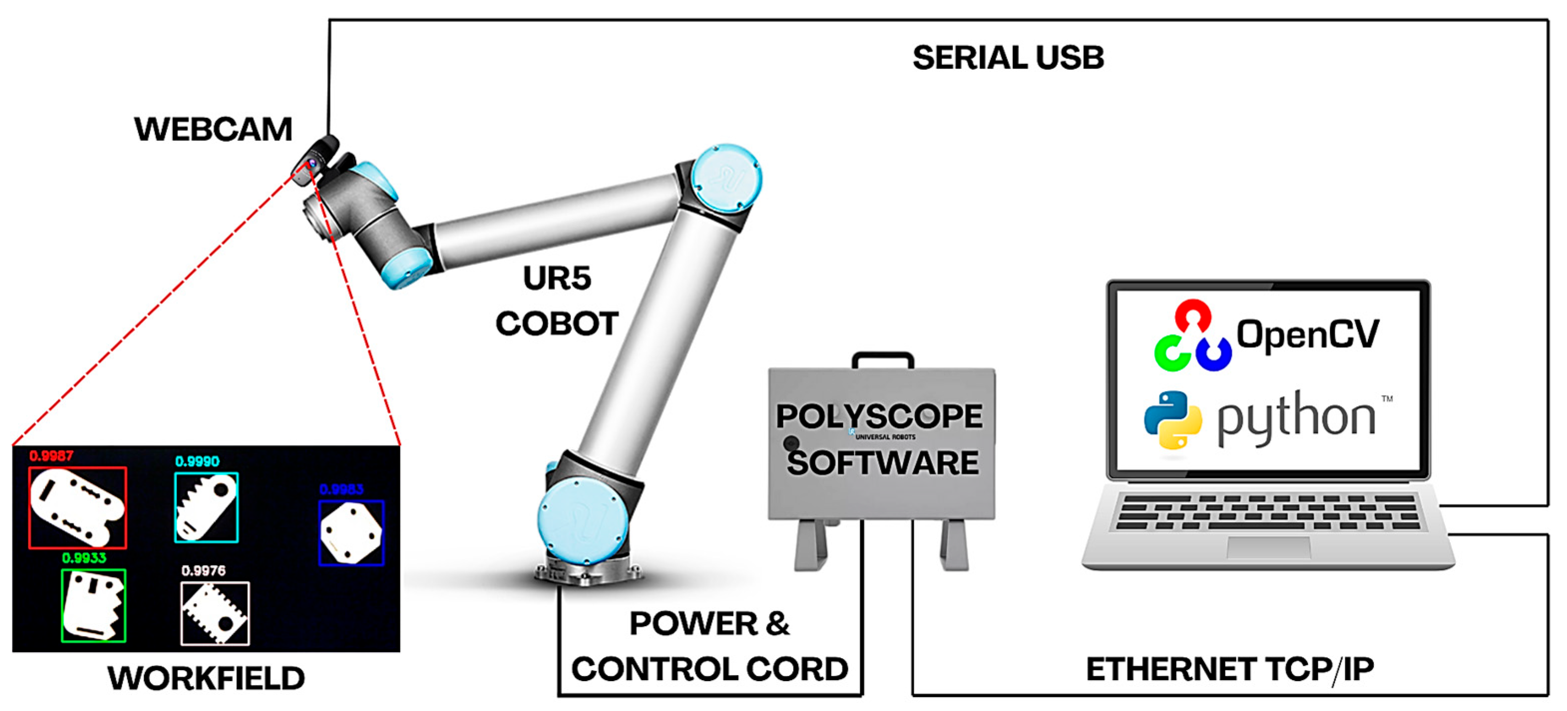
The purpose of the research work was to develop and set up a robotic sorting workstation [Figure 1]. The implementation was based on the use of a Universal Robots UR5 cobot robotic station and open-source software.

The cell was equipped with a Universal Robots UR5 robotic arm, which featured six degrees of freedom, a maximum payload of 5 kg, and an 850 mm reach. The UR5 robot meets the criteria for classification as a collaborative robot (cobot). This type of design allows for less stringent safety precautions during its interaction with the operator. The robot was controlled via a CB1 generation controller running software version 1.8. 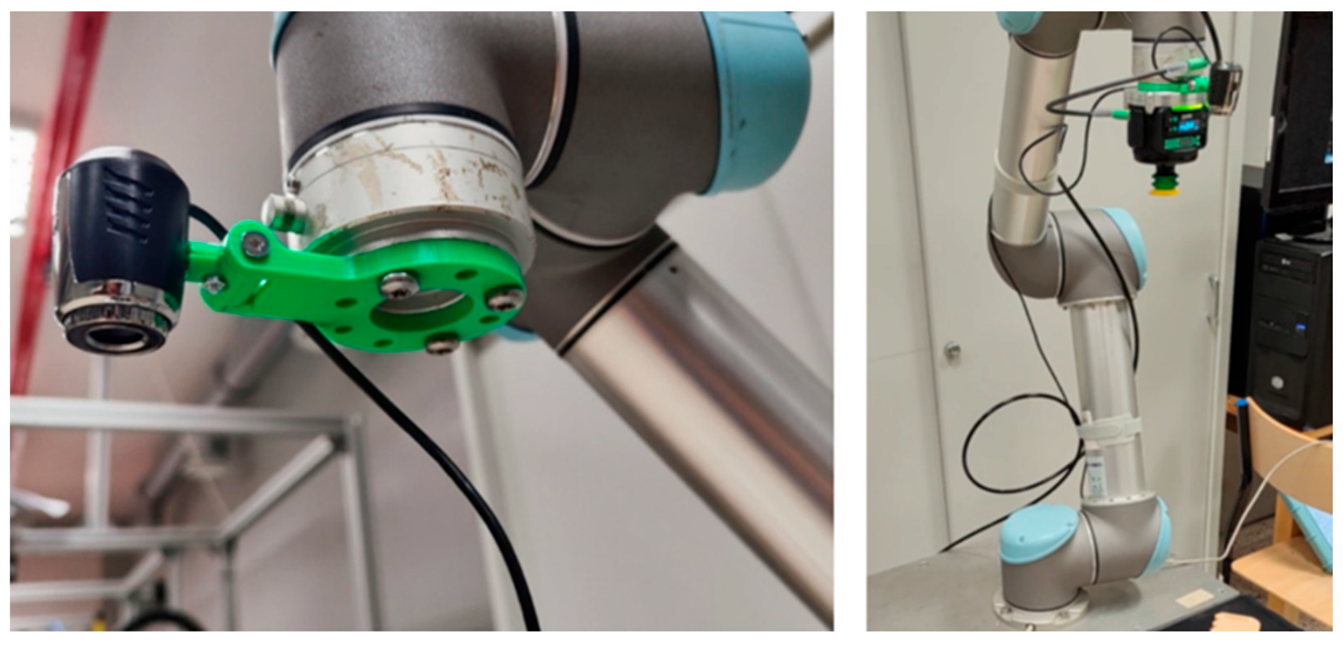The cobot has been equipped with a piCobot vacuum gripper by PIAB [Figure 2], a dedicated device engineered to attach directly to the flange of Universal Robots’ cobots, with a grip payload of up to 7 kg.

The webcam [Figure 2] used in this setup was the Esperanza EC105, a USB 2.0 device with a 1.3-megapixel CMOS sensor capable of delivering HD video. The webcam offers 24-bit true color and supports automatic white balance, exposure, and color compensation, along with manual focus, adjustable from 5 cm to infinity. The camera was attached to the cobot’s flange using a dedicated bracket printed on a 3D printer. This mount allowed the camera to be attached between the robot’s flange and the vacuum gripper. As a result, a connection between the camera and the robot in an eye-in-hand configuration was achieved.

No specialized hardware was necessary for the video system—all functionality was implemented on a standard PC running a Windows 10 system with an Intel Core i5-10310 processor. A single USB port (for the camera’s serial connection) and a single RJ45 port (for the Ethernet link to the cobot controller) were sufficient to connect the external devices.

The core element of the designed station was a PC-based vision system developed entirely in Python 3.12. The implementation leverages Python’s built-in modules—such as socket, threading, logging, time, os, pathlib, random, re, and math, etc.—along with several specialized external libraries. Specifically, the system utilizes OpenCV (version 4.10.0.84) for computer vision, NumPy (version 1.26.4) for numerical computations, scikit-learn (version 1.5.0) for machine learning, scikit-image (version 0.23.2) for image processing, joblib (version 1.4.2) for parallel processing, and glob2 (version 0.7) for enhanced file system operations.

The developed vision system was implemented on a Windows-based platform, which does not fulfill real-time system (RTS) requirements. While multithreading was used to allow parallel execution of robot communication and image processing tasks, the system does not guarantee deterministic timing. For reference, the average processing time for one cycle is approximately 1250 ms, broken down as follows:

• Image acquisition: ~100 ms.
• Identification process (MLP/classical method): ~1100 ms.
• Object localization: ~50 ms.

The application orchestrates the entire processing pipeline, which includes the following:

• Image acquisition: capturing images from a webcam.
• Initialization procedures: executing camera calibration to determine distortion parameters and performing hand–eye calibration to align the camera and robot coordinate systems.
• Image processing and analysis: analyzing image data within a defined ROI to extract meaningful information.
• Control integration: making decisions based on the processed data and transmitting corresponding motion commands to the UR5 cobot’s execution arm.

This structured approach ensures that all components—from sensor data acquisition to robotic actuation—are cohesively integrated within the Python-based framework.

The webcam was interfaced with the vision system using a serial USB protocol. A dedicated function was implemented to manage data handling and image acquisition in a separate execution thread. The camera connection was established using the VideoCapture() function from the OpenCV library. The function accepted two synchronization primitives of type threading.Event(), namely frame_event and stop_event, as well as a dictionary frame_storage, which was used to store the captured frames. This design enabled the camera function to operate asynchronously in a dedicated thread while maintaining seamless communication with other threads invoking it.

A custom communication setup was implemented, in which a client was developed on the robot controller to interface with an external server (a PC running Python software). Additionally, a dedicated function-handling structure was designed on the robot controller to process incoming command strings from the server. The framework for controlling the robot was implemented within the Polyscope 1.8 environment on the cobot’s controller using the URScript scripting language. This language provided the necessary functions to manage the execution arm. Each function was invoked by a string format command received by a client on the robot controller from a server managed by the vision system. The implemented functions enabled operations such as performing MoveJ commands to predefined coordinates, executing MoveL movements based on specified displacements, toggling the vacuum gripper, or retrieving the current TCP coordinates, etc.

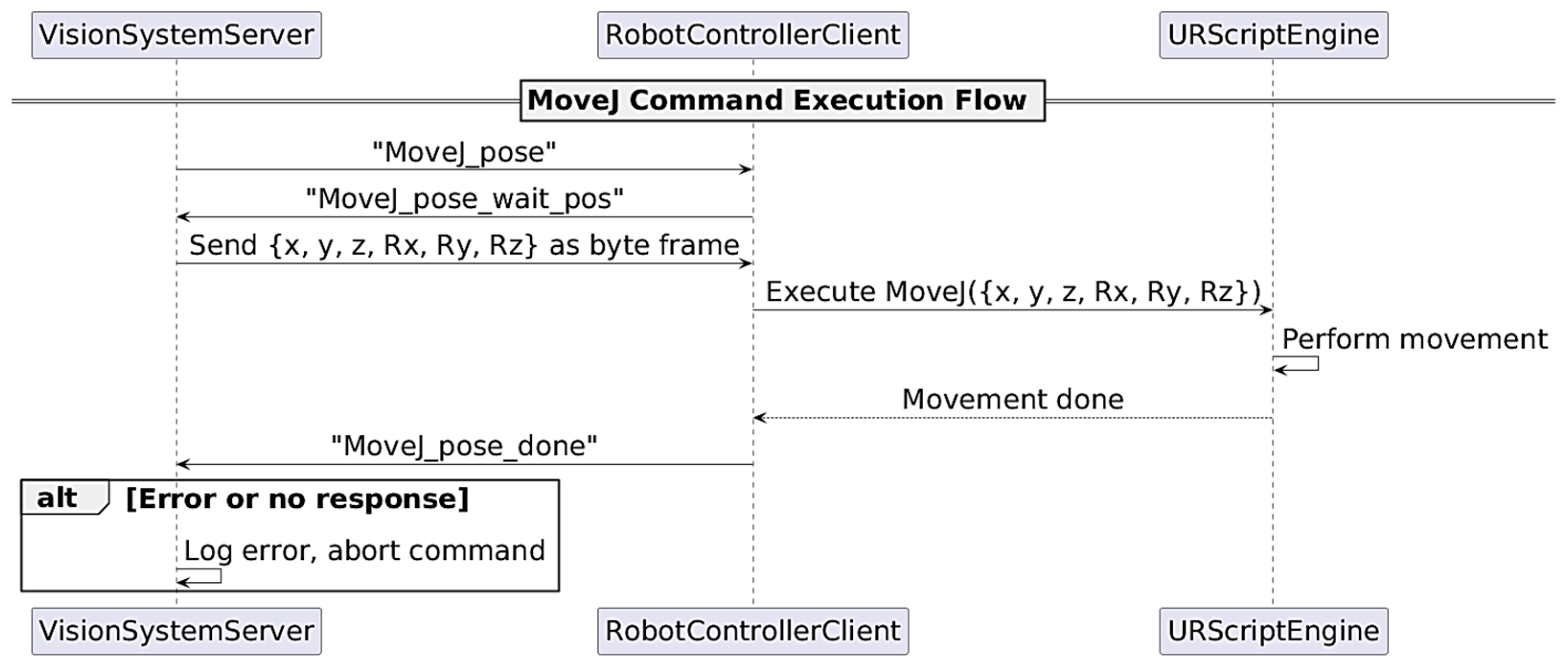
Every function that produced a physical effect was implemented using a handshake protocol. For instance, a MoveJ command was initiated by the vision system server, sending a “MoveJ_pose” command, to which the client responded with a “MoveJ_pose_wait_pos” handshake. Subsequently, the server transmitted the target {x, y, z, Rx, Ry, Rz} coordinates encoded in a byte frame and awaited confirmation of successful command execution via a “MoveJ_pose_done” response. In cases of an incorrect or absent response, the vision system treated the move command as unsuccessful or erroneous and aborted the operation with appropriate error logging. It was noted that although UR robots provide dedicated error-handling mechanisms via error frames on specific ports (e.g., port 30003), this functionality was not implemented in our proof-of-concept solution. Below is a presented UML diagram example of controlling the MoveJ movement to a specific position [Figure 3].

The block diagram [Figure 4] illustrates the key steps and the flow of data between the different modules. The flowchart reflects the logical structure of the program, starting with system initialization, camera calibration, and hand–eye calibration, with a simplification of the part of the program responsible for sorting.

At the program initialization stage, based on the values of variables set by the user, a decision is made to take a new series of images for camera calibration and hand–eye system calibration or to use data stored in a user-defined file path. Then, when the robot is in the observation position of the working field, the program takes a picture and expects the user to define the ROI area of interest. After obtaining the camera’s internal parameters, the rotation and translation matrix between the camera and the gripper’s TCP point, and the ROI coordinates, the program proceeds to call the infinite loop subroutine responsible for identifying objects and sorting them.

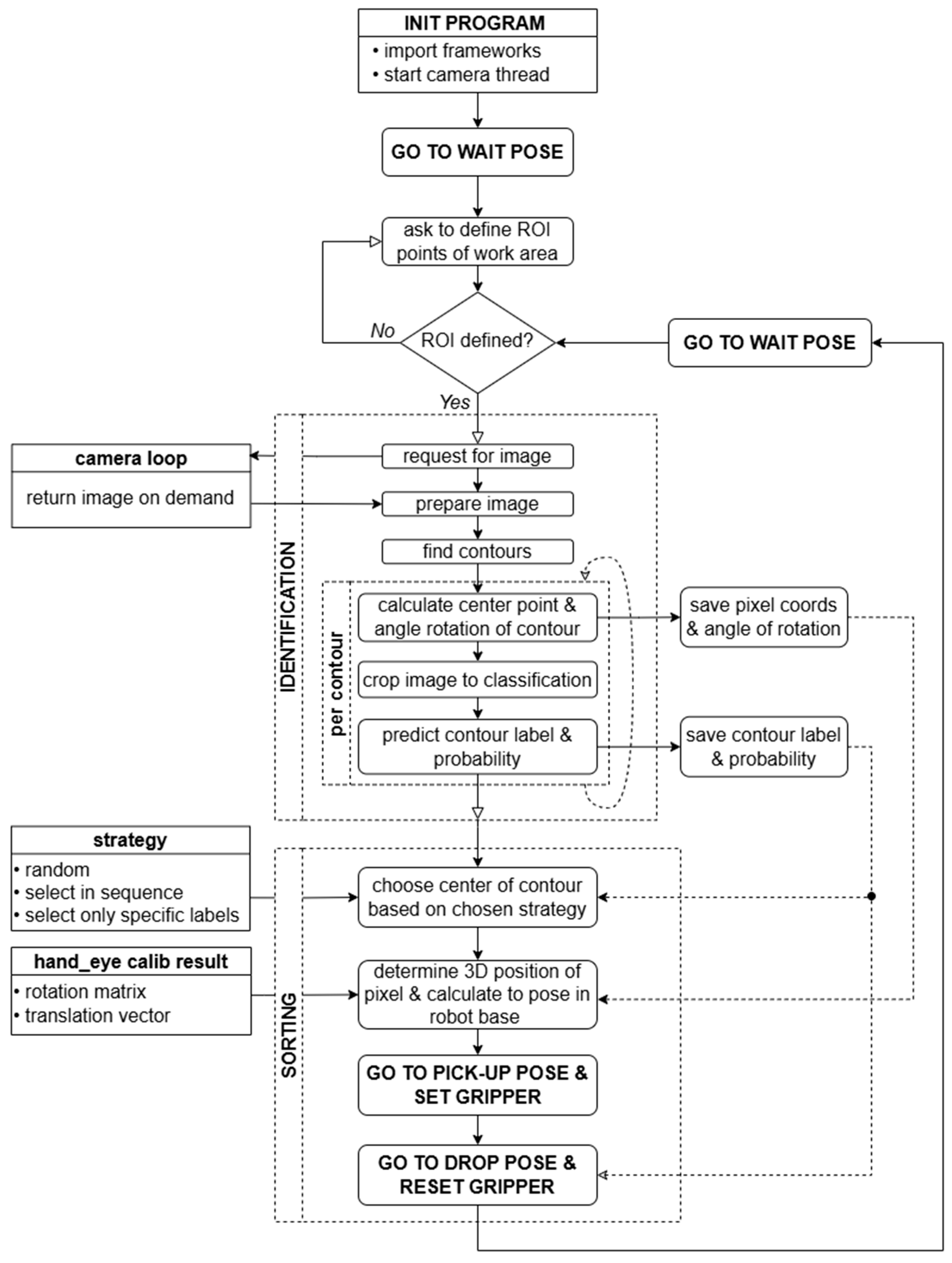
A block diagram [Figure 5] illustrating the operation of the subroutine responsible for object identification and sorting in an infinite loop is presented below. This subroutine operates in a continuous mode, which makes it possible to automate the process in the form of image data acquisition, image processing, decision-making based on object identification, and generation of control commands for the cobot controller.

The operation scheme of the infinite loop can be divided into two main stages: identification and sorting. During the first stage, when the robot is in the observation position, an image retrieval signal is sent to the camera thread. The program then processes the received frame—removes distortion, converts the image to grayscale, ignores the background outside the working field, and then detects shapes using contour detection. For each contour detected, the program determines its geometric center of gravity and angle of rotation relative to the camera’s coordinate system. For each shape, an object identification process is also carried out using a pre-trained MLP classifier model. All this data (prediction and prediction coefficient of the objects, coordinates of their geometric centers of gravity, and rotation angles) is passed to the component functions of the second stage—sorting. There, in the first step, the most suitable object for manipulation is extracted using the selected strategy. Then, using inverse projection, the 3D coordinates of the geometric center of gravity of this object are determined, and the cobot is sent to the designated position to retrieve it. Based on the identification, the position of the stack for depositing the sorted objects is also determined. After the object is successfully sorted, the robot returns to the observation position, and the identification loop cycle is completed.

It is worth mentioning the sorting strategies employed, which were depicted in the diagram as an input argument to the program’s SORTING state. The software implemented three selection scenarios for items designated for manipulation:

• Random selection—a random element was chosen from all identified elements;
• Sequential selection—elements were selected in ascending order from all identified elements (e.g., labels from 1 to 5);
• Label-specific selection—only elements identified with a predefined label were selected.

This functionality was introduced to facilitate testing and potential debugging, to evaluate the impact of changing the selection strategy on the overall effectiveness of the algorithms, and, most importantly, to demonstrate the solution’s flexibility in the production process. By continuously processing data on identified objects, the system could adapt to current production needs by prioritizing the sorting of objects in higher demand on the production line at any given time.

3. Methodology

The purpose of the research work was to develop and program a robotic sorting station capable of performing automated and repetitive operations based exclusively on the image acquired from a webcam mounted on the robot’s flange. The system was required to accurately identify objects based on analysis of their 2D shapes and to determine the position of the objects to be picked within the robot’s workspace. The developed software enabled the fully automated operation of the station in a research and development environment. The primary functionalities implemented in the software included camera calibration, camera–robot calibration, and the execution of the sorting program logic. It should be noted that the work did not focus on comprehensive error handling or the adaptation of the application for use in an industrial environment, as the project was conceptual and intended solely for research purposes to fulfill the assumed requirements.

The initial stage necessary for the implementation of image processing algorithms is camera calibration, which primarily aims to eliminate distortions caused by the optical system. The calibration procedure involves capturing multiple images of a calibration board from various angles and positions. In the proposed system, this process was automated through dedicated functionality within the vision system. The six-axis robot sequentially moved to a predefined set of positions and captured images of the working area. Images in which the calibration chessboard of the specified dimensions was not detected or was only partially detected were automatically discarded. The remaining valid images were then utilized to compute the camera calibration parameters. The calibration process was conducted using the calibrateCamera() function provided by the OpenCV library. The calibration chessboard used in this process had the following dimensions: 420 mm x 380 mm. The determined intrinsic camera parameters and distortion coefficients for the used webcam are presented in [

Table 1. Obtained camera parameters and distortion coefficients after camera calibration process.

Camera Calibration Python Results	Values
Camera matrix	[[760.24388432	0.		293.69701361]
	[0.	760.8296185		279.03151807]
	[0.	0.		1.]]
Distortion coefficients	[[−1.62921574 × 10−1	1.13593220 × 10−1		6.76147908 × 10−4
	1.68617740 × 10−4		−3.46985533 × 10−1]]

].

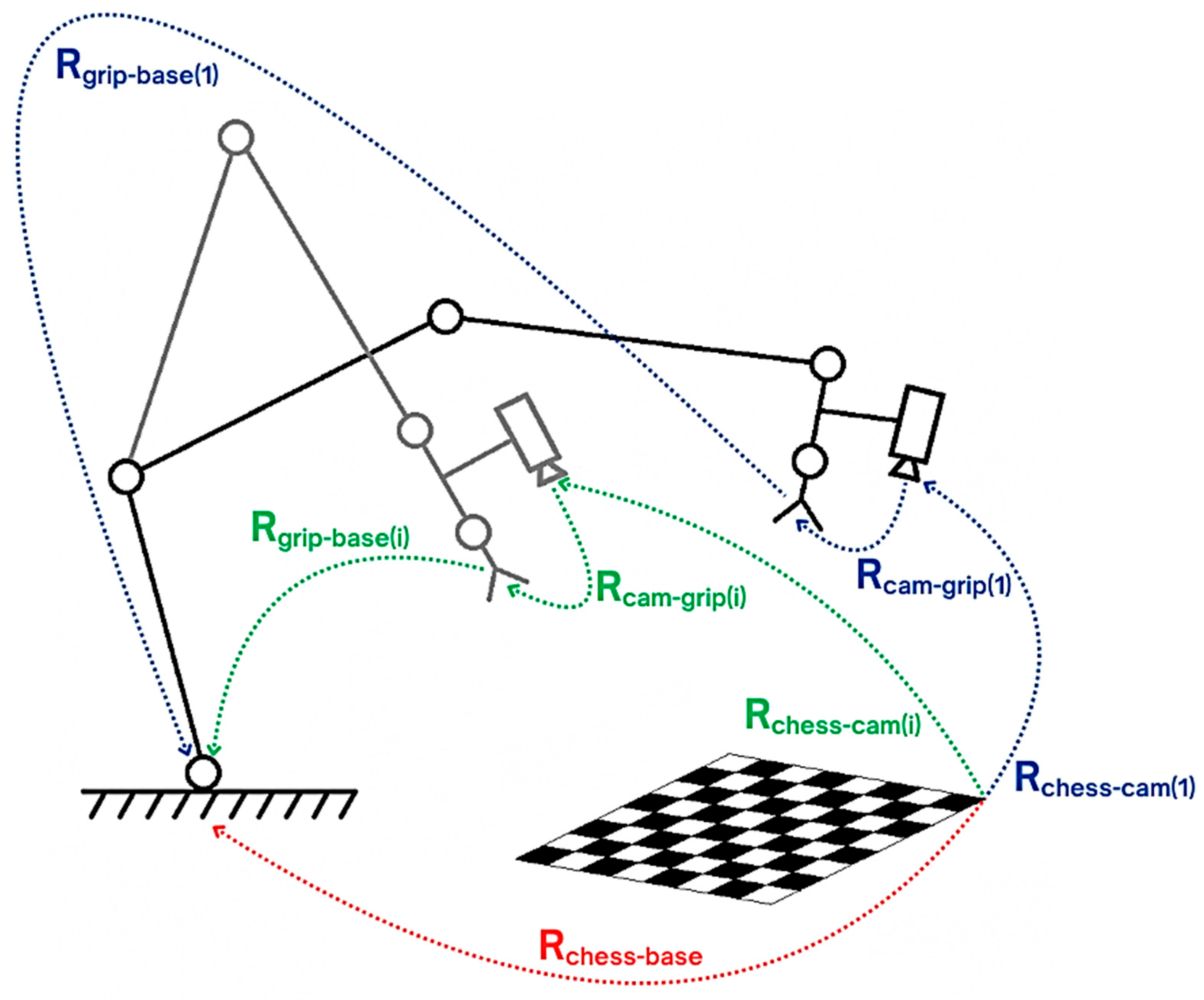
The calibration of the camera to the robot was the next step necessary to handle the precise object manipulation in space. This process established a spatial relationship between the camera coordinate system and the robot’s TCP point coordinate system by determining the rotation matrix and translation vector linking them together [Figure 6]. For the camera-to-robot calibration task, the hand–eye calibration method was implemented in an eye-in-hand configuration [55]. For this purpose, a dedicated functionality was developed within the vision system software. This functionality automated the acquisition of multiple images of a calibration checkerboard at various robot poses while simultaneously fetching the manipulator’s positions at the moments when the images were captured. Positions were obtained by querying the robot controller using the get_actual_tcp_pose() function from URScript, providing the transformation Rgrip-base(i) for each iteration. At the same time, the transformation Rchess-cam(i) was estimated using the solvePnP() algorithm based on the detected checkerboard pattern in the image. The software continuously verified the visibility and readability of the checkerboard pattern in the captured images. Any images where the checkerboard was partially occluded or unreadable, along with their corresponding poses, were discarded from the data to ensure calibration accuracy.

The hand–eye calibration process aimed to determine the transformation Rcam-grip between the camera and the robot’s end-effector. The method relies on a set of paired transformations, Rgrip-base(i) and Rchess-cam(i), acquired through multiple iterations. The calibration assumes that Rchess-base (the pose of the checkerboard relative to the robot base) and Rcam-grip (the camera-to-gripper relationship) remain constant during the entire process.

From the set of valid images, the detected checkerboard patterns were analyzed. The rotation matrices and translation vectors describing the checkerboard’s position relative to the camera were calculated using the solvePnP() function from the OpenCV library. Concurrently, the rotation matrices and translation vectors representing the robot’s TCP position relative to the robot’s base coordinate system were retrieved from the recorded TCP pose values. Using these paired sets of rotation matrices and translation vectors, hand–eye calibration was performed utilizing the calibrateHandEye() function in OpenCV. The resulting rotation matrices and translation vectors were computed for all available hand–eye calibration methods implemented in the OpenCV function, including Tsai–Lenz [56], Park–Martin [57], Horaud–Dornaika, and Daniilidis [58].

Table 2. Summary of the obtained spatial dependencies in accordance with the methods used.

Hand–Eye Calibration Methods Python Results		Values
Tsai–Lenz	Rotation matrix	[[0.9991 −0.0152 0.0388] [0.0137 0.9993 0.0382] [−0.0393 −0.0376 0.9985]]
	Translation vector	[[0.0017] [−0.0803] [−0.1302]]
Park–Martin	Rotation matrix	[[0.9992 −0.0130 0.0388] [0.0116 0.9992 0.0369] [−0.0392 −0.0364 0.9986]]
	Translation vector	[[−0.0022] [−0.0796] [−0.1318]]
Horaud–Dornaika	Rotation matrix	[[0.9991 −0.0129 0.0388] [0.0115 0.9993 0.0368] [−0.0392 −0.0363 0.9986]]
	Translation vector	[[−0.0022] [−0.0796] [−0.1318]]
Daniilidis	Rotation matrix	[[0.9992 −0.0141 0.0383] [0.0124 0.9991 0.0413] [−0.0389 −0.0408 0.9984]]
	Translation vector	[[−0.0059] [−0.0855] [−0.1293]]

presents an example of the resulting rotation matrix and translation vector obtained using all the methods mentioned, which illustrates the spatial relationship between the camera and the robot’s defined TCP point. As the discrepancies achieved with all methods were negligible, a fundamental version based on the Tsai–Lenz method was chosen.

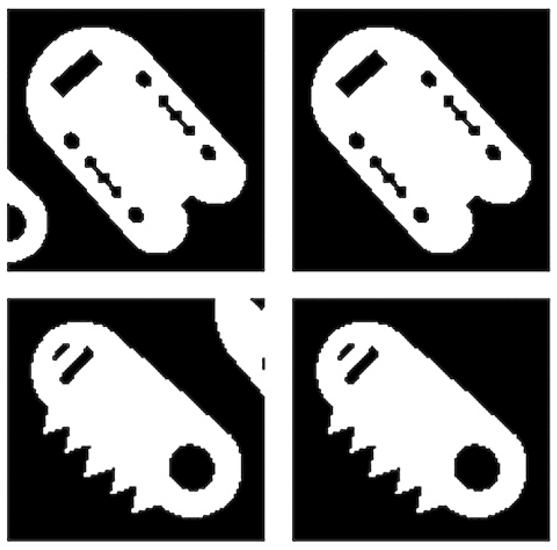
The data used for object identification was entirely acquired from a webcam mounted on the robot’s flange. All objects used were fabricated using light-colored filament, making them strongly distinguishable against a contrasting dark background. The raw images captured by the webcam underwent a series of preprocessing steps. Initially, distortion correction was applied by utilizing precomputed intrinsic camera parameters to remove lens-induced distortions [Figure 7]. Subsequently, the images were converted to grayscale to simplify further processing. The next step involved binarization, transforming grayscale images into a binary format. Various binarization techniques were assessed during the development phase, including standard thresholding, adaptive thresholding, Otsu’s method, and an approach incorporating the binarization step from Canny edge detection without the edge-linking stage. Empirical analysis demonstrated that standard thresholding was both sufficient and optimal for the intended application.

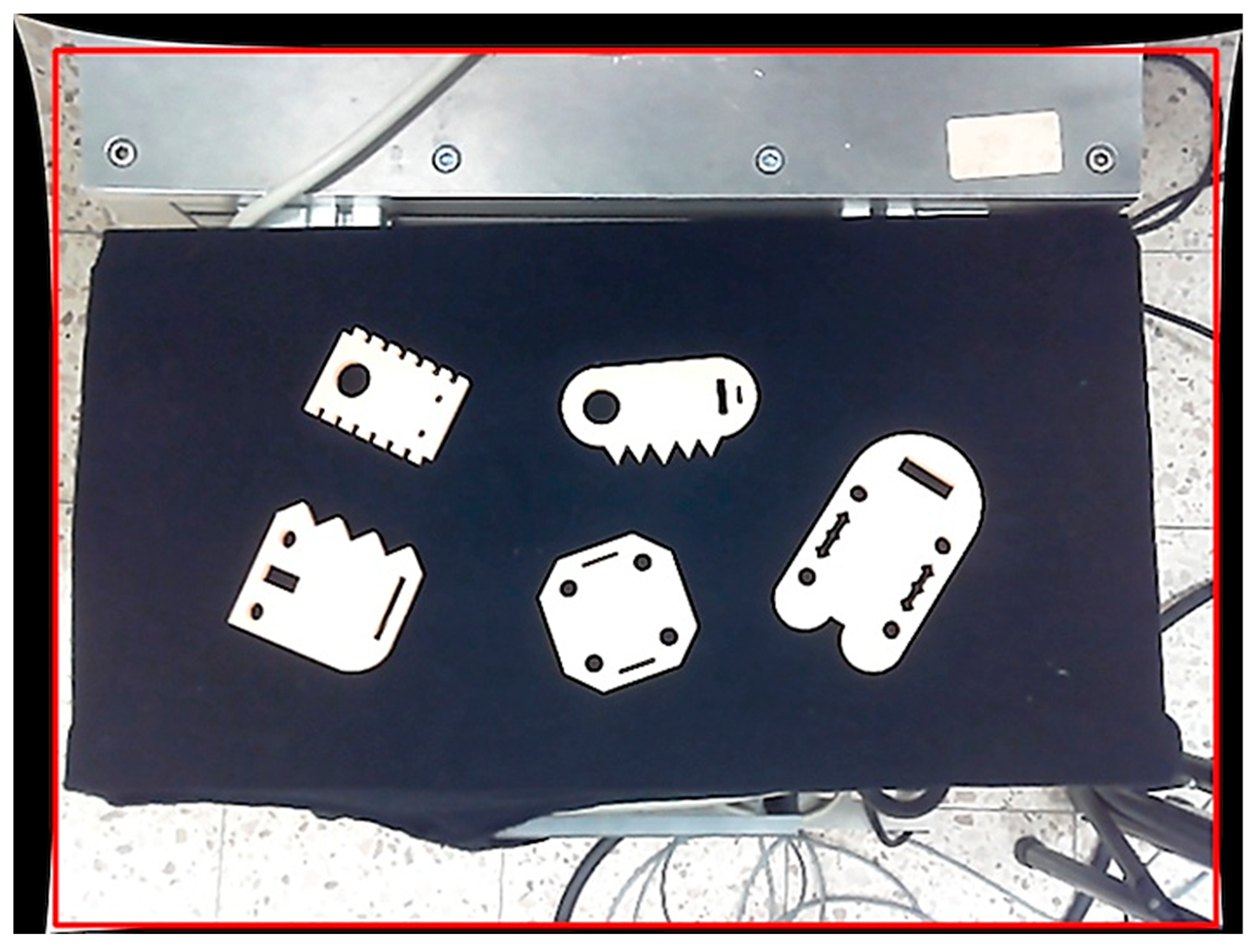
After preprocessing, the image captured at the observation position contained not only the workspace but also irrelevant visual information. To eliminate this, a function was developed to define the working field contour and exclude the unnecessary background. During the position setup phase, the robot moved to the predefined observation position, prompting the application to await operator input for defining multiple points on the camera image that outlined the Region of Interest (ROI). These points were then used to create a polygonal mask and effectively isolate the ROI by applying a bitwise AND operation to suppress the background [Figure 8].

Further functionality was developed to preprocess data using contour detection, allowing the extraction of images containing only the analyzed shapes. On the preprocessed image, the system invoked OpenCV’s findContours() function to detect object contours [Figure 9]. The pixel coordinates of each detected contour were then used to generate the dataset. Using OpenCV’s boundingRect() function, the coordinates of the bounding rectangle enclosing each contour were obtained, with an additional margin parameter taken into account. 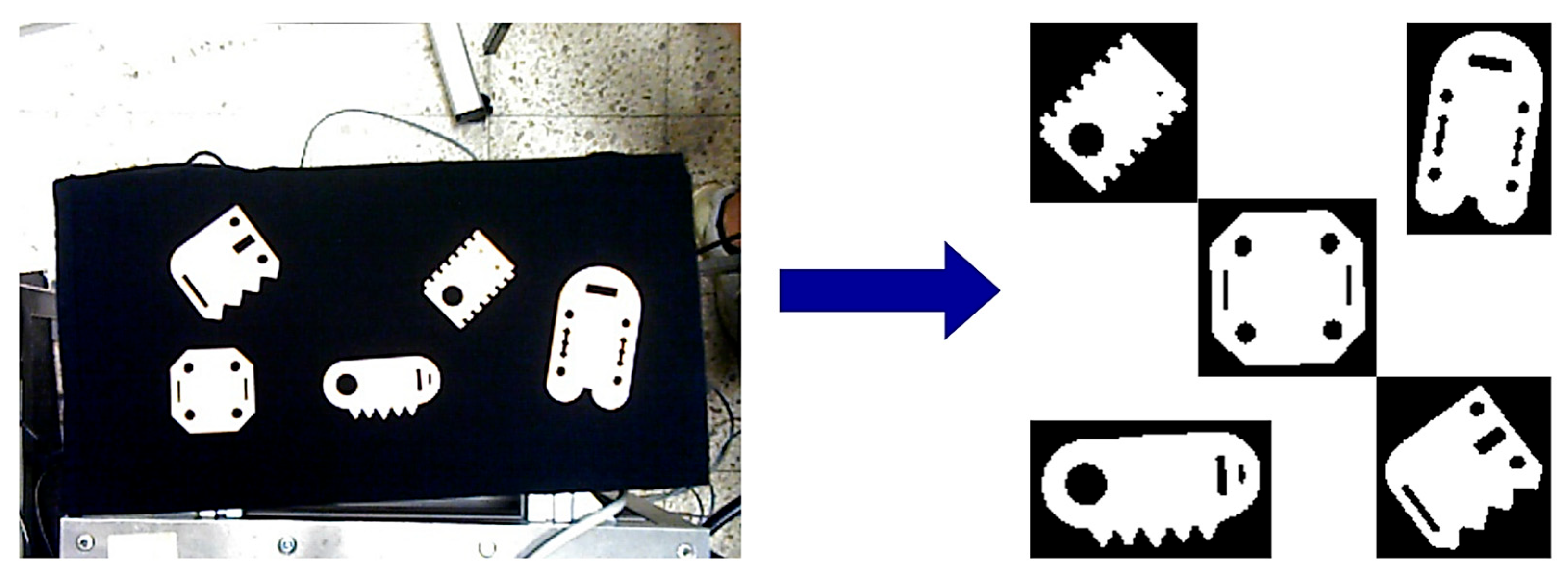Since bounding rectangles of individual objects could interfere with each other, a mechanism was also implemented to ignore areas outside the analyzed contour, employing a bitwise AND operation process [Figure 10], analogous to the background exclusion. Finally, the program aggregated cropped images corresponding to the designated bounding rectangles along with their coordinates for visualization purposes.

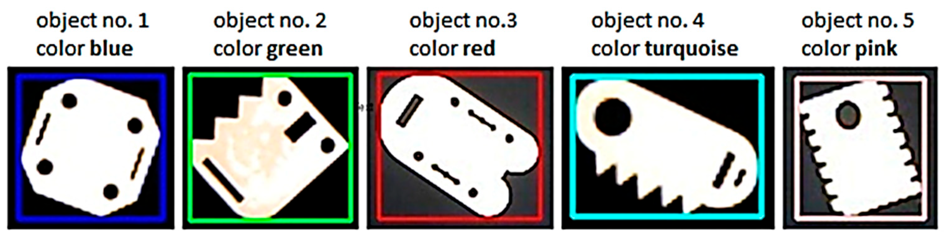
The dataset [Figure 11] prepared through this process served as a unified input for all identification methods, including contour similarity analysis, feature descriptor matching, and, most importantly, the training and subsequent utilization of a Multi-Layer Perceptron (MLP) classifier for shape identification.

The first identification method analyzed was contour similarity. This approach involved selecting reference images of shapes intended for sorting, preprocessing them, and extracting their contours (outer and inner) with findContours() function. These reference contours served later as the baseline for subsequent comparisons during the system’s automated operation. Once an image of the workspace was acquired, the vision system processed it to extract the contours of detected objects (dataset), which were then compared against the reference contours.

Contour comparison was performed using OpenCV’s matchShapes() function. This function calculates similarity coefficients based on Hu moments, which are derived from normalized central moments. Hu moments offer invariance to translation, rotation, and scaling—properties that make them particularly effective for shape recognition in computer vision. Three different algorithms (CONTOURS_MATCH_I1, CONTOURS_MATCH_I2, and CONTOURS_MATCH_I3) were available to compute these similarity values according to distinct mathematical formulations [59].

$$\left\{\begin{array}{c}{m}_i^A=sign\left(h_i^A\right)·\mathit{log}{h}_i^A\\ m_i^B=sign\left(h_i^B\right)·\mathit{log}{h}_i^B\end{array}\right.$$

(1)

where $h_i^A$ and $h_i^B$ are the Hu moments of shapes A and B.

Formula for the CONTOURS_MATCH_I1 method (2).

$$I_1\left(\mathrm{A},\mathrm{B}\right)=\sum _{i=1..7}\left|{\displaystyle \frac{1}{m_i^A}}-{\displaystyle \frac{1}{m_i^B}}\right|$$

(2)

Formula for the CONTOURS_MATCH_I2 method (3).

$$I_2\left(\mathrm{A},\mathrm{B}\right)=\sum _{i=1..7}\left|m_i^A-m_i^B\right|$$

(3)

Formula for the CONTOURS_MATCH_I3 method (4).

$$I_3\left(\mathrm{A},\mathrm{B}\right)=\sum _{i=1..7}{\displaystyle \frac{\left|m_i^A-m_i^B\right|}{\left|m_i^A\right|}}$$

(4)

Based on the analysis of the shapes selected for sorting, a two-step procedure for shape identification using contour similarity was developed. For this purpose, the findContours() function was employed in RETR_TREE mode to extract the pixel coordinates of all contours, preserving both external and internal contours along with their hierarchical relationships. In the first identification step, only the external contours were compared against the corresponding external reference contours. In the subsequent stage, the ideal approach was to compare internal contours—subordinate to a given external contour—against the corresponding internal reference contours. In a proper implementation, each detected internal contour would be matched with its most similar internal reference contour, and the best match would be removed from the reference pool to prevent duplicate assignments.

At each stage of matching both external and internal contours, no single method was employed. Instead, the identification process was based on the arithmetic mean of the results obtained from all three methods. There was no detailed comparison conducted between the outcomes of the individual methods and those derived from the arithmetic or variably weighted means. However, during the functional design phase, intuitive tests based on contour similarity revealed that using the arithmetic mean yielded significantly greater stability—manifested by fewer false negatives and false positives—as well as a higher rate of correct identifications compared with using any individual method.

The second identification method analyzed was feature descriptor matching. The approach involved selecting reference images of shapes intended for sorting, preprocessing them, and extracting their cropped images. These processed reference images later served as a reference point for subsequent comparisons during automated system operation. Once an image of the work area was captured, the vision system processed it to extract cropped images of detected objects (dataset), which were then compared with the reference images.

Feature descriptor matching was performed using the SIFT algorithm in combination with FLANN-based matching. The SIFT detector was instantiated using OpenCV’s SIFT_create(), which computed keypoints and descriptors for both reference and object images. For the FLANN matcher, parameters were configured with the algorithm set to use the KD-Tree (FLANN_INDEX_KDTREE, value 1) with five trees and search parameters defined with 10 checks. The matcher then employed the knnMatch() function with k = 2 to retrieve the two best matches for each descriptor. A ratio test was applied using a threshold value of 0.7 (GOOD_MATCH_RATIO), whereby a match was considered valid if the distance of the best match was less than 0.7 times that of the second-best match. Additionally, a minimum match count of 20 (MIN_MATCH_COUNT) was required to confirm a valid match, thereby ensuring robustness against false positives.

For each detected object, SIFT-based matching was performed against the corresponding reference image. Matches that met the specified criteria were aggregated, sorted in descending order by the number of good matches, and then visualized using OpenCV’s drawMatches() function. Diagnostic overlays were added to the visualizations to indicate the reference name, binarization method, match counts, and the observed minimum and maximum ratio values.

The last identification method analyzed was classifying the detected shapes using an MLP classifier. This functionality involved the collection of a greater reference data range for training and validating the neural network-based classifier. A camera mounted on the robot’s flank, positioned at the observation point, was used to manually capture approximately 150 images of each object in various positions and rotations on the workspace. The images were subsequently organized into separate folders corresponding to each shape. To efficiently prepare the data for analysis, a dedicated module was developed that used os.walk to iterate image files in shape-specific directories, process the images through preprocessing algorithms, and prepare unified data. The processed data was stored in a separate folder with an equal folder hierarchy.

To train the neural network classifier, a dedicated training module was implemented. This module featured a function that loaded images from a specified folder corresponding to each label. The function iterated over all image files in the folder and resized them to a fixed square dimension using transform.resize. Each resized image was then flattened into a one-dimensional vector via the skimage.io.flatten() method. The function returned two lists containing the processed image vectors and the corresponding label. This procedure was executed for each folder, and the resulting lists were concatenated to form an aggregate dataset for the images and labels. This dataset was subsequently partitioned into training and validation sets using scikit-learn’s train_test_split() function, with 20% of the data allocated for validation and the remaining 80% used for training.

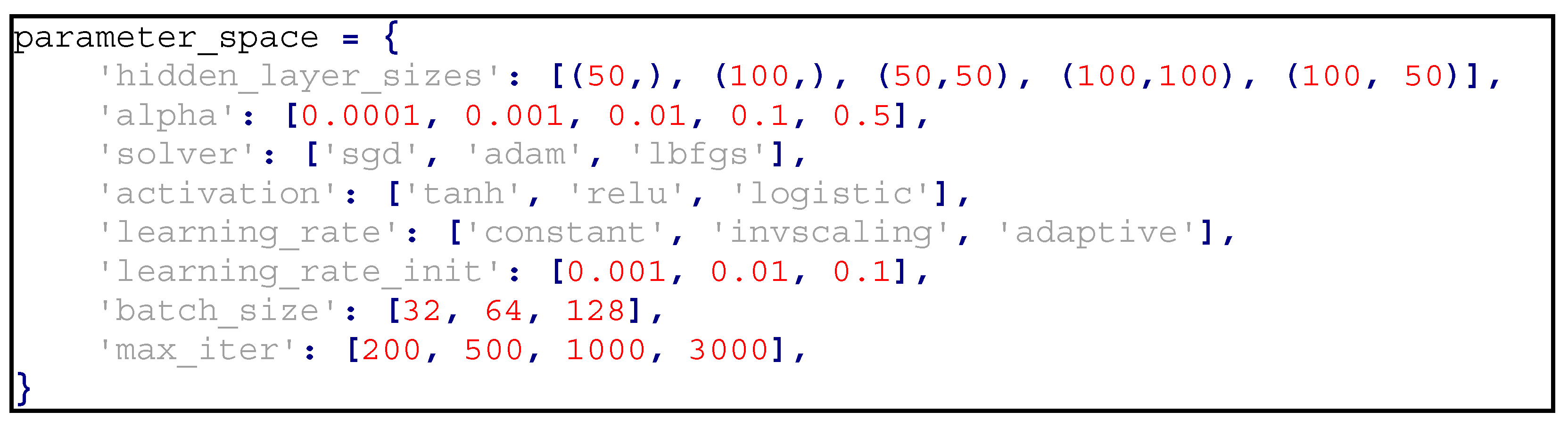
To optimize the learning process, the RandomizedSearchCV approach was used, streamlining the process of optimizing the classifier’s hyperparameters. An MLP classifier instance was created with random state 42 and early stopping enabled. The distribution of parameters to be sampled included different configurations for hidden layer sizes, alpha values, solvers, activation functions, learning rates, initial learning rates, batch sizes, and maximum iterations. RandomizedSearchCV was executed with 100 iterations (n_iter = 100), using all available processors (n_jobs = −1) and performing five-fold cross-validation (cv = 5). The model was then fitted to the training data. Below is a matrix of hyperparameters considered by the RandomizedSearch methodology during the optimal learning process:

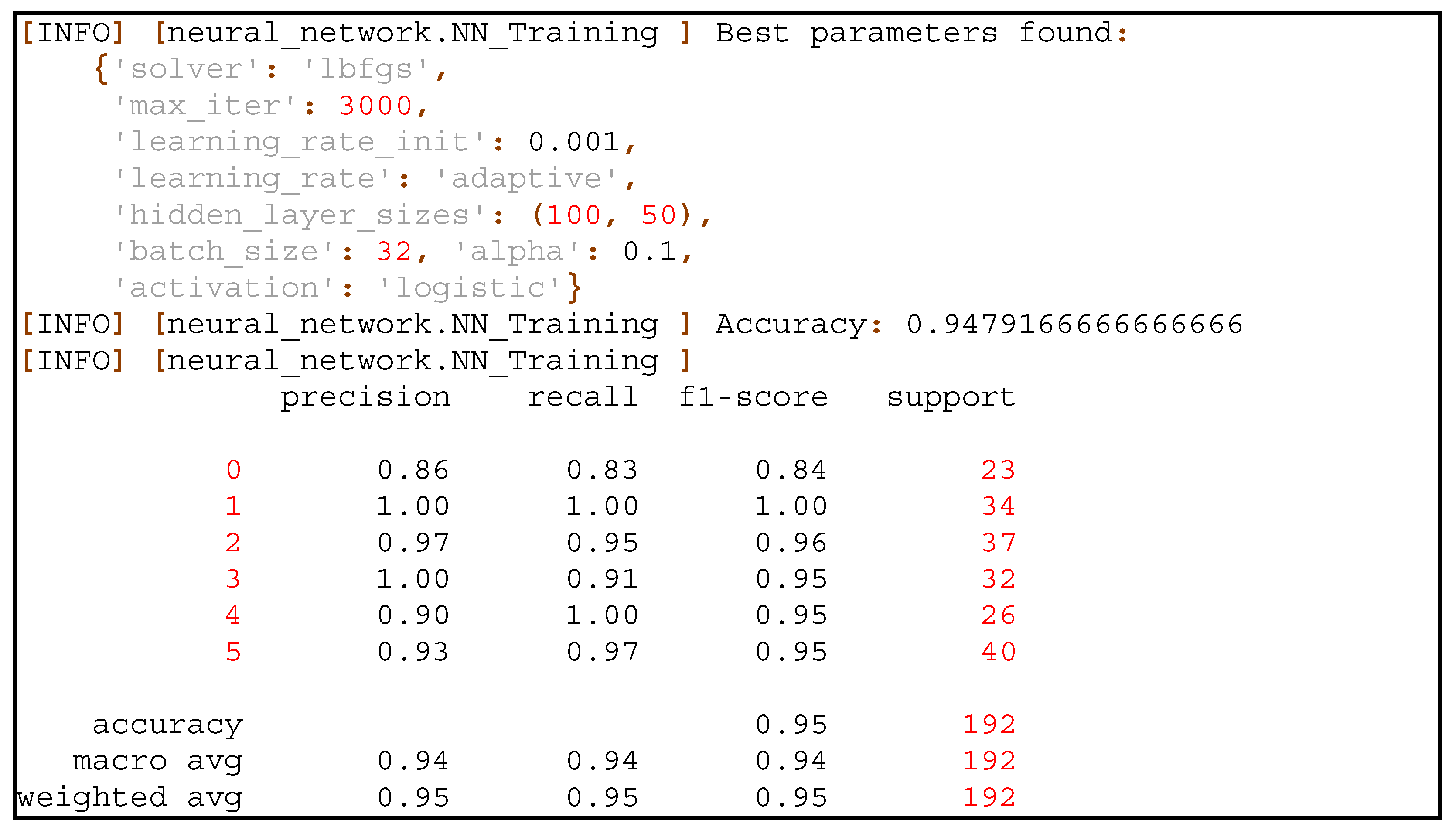
After the random search was completed, the best parameters were identified, and the performance of the classifier was evaluated on the validation set. The accuracy score was calculated, and a classification report was generated. In addition, the top 10 models, ranked by average test score, were selected and saved using joblib.dump, ensuring and simplifying future use. The following lines are a log snippet of the report showing the set of hyperparameters obtaining the most optimal results and the results they obtained:

The chosen classifier was integrated into the program, enabling automated operation within the sorting system. The classifier’s workflow involved processing input images using the same preprocessing pipeline as during training—resizing to a square format followed by flattening into a vector representation, then generating predictions, and visualizing the results as well. Based on the processed input, the function returned the most probable label alongside the corresponding confidence score. The classification results obtained at this stage were part of the data aggregated by the sorting loop program.

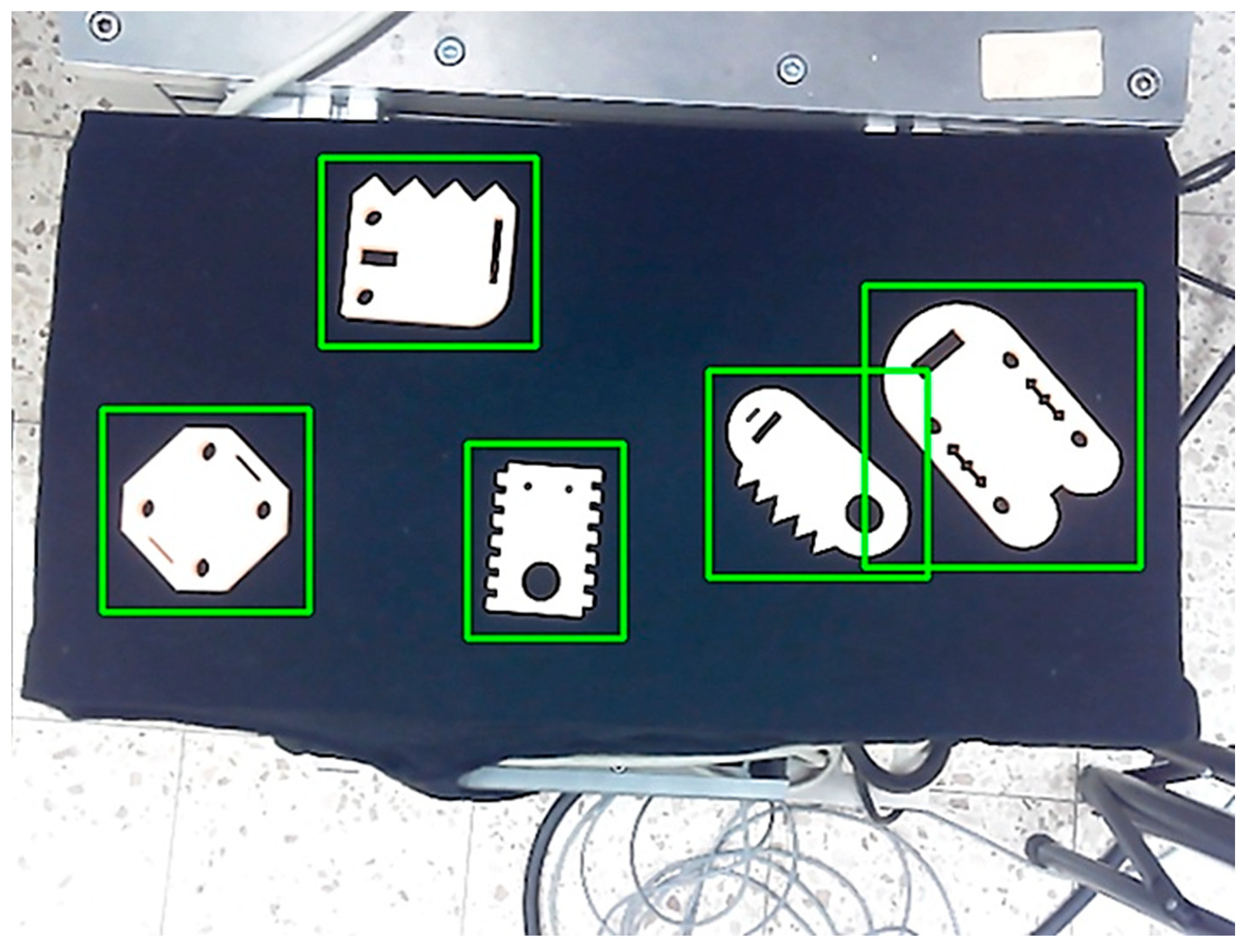
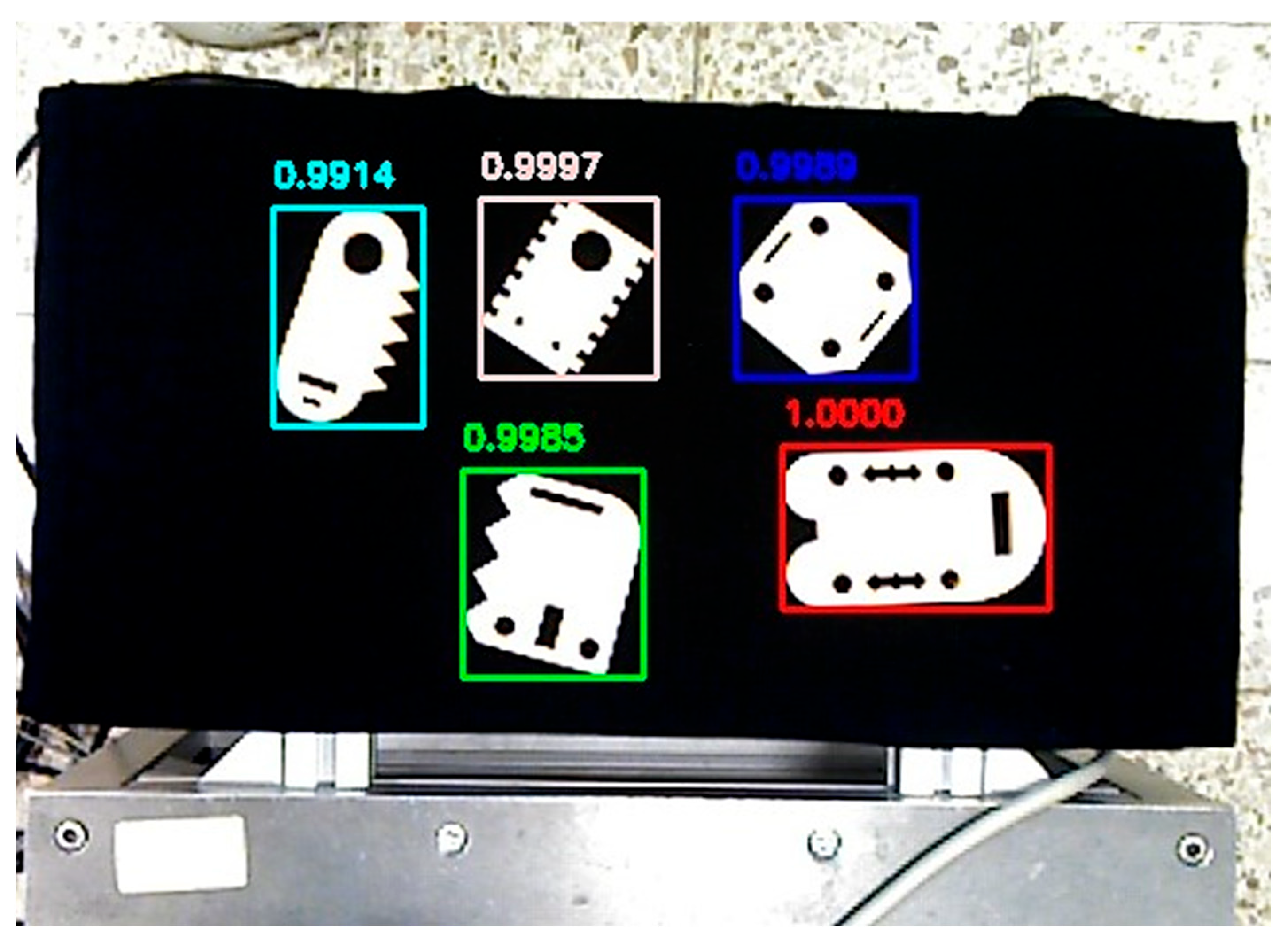
For visualization, the system annotated the processed images by drawing bounding boxes around detected shapes and overlaying classification results [Figure 12]. Classified shapes were highlighted using predefined colors corresponding to their labels. The processed images provided feedback on the classification performance and facilitated the validation.

Regardless of the chosen identification method, the final step in enabling the robot to perform its task was to develop a method for determining the position of objects within the robot’s coordinate system. As the system used a webcam to capture two-dimensional images, reconstructing a three-dimensional position from these images was a non-trivial task. It was decided to use an approach where a single global position with a determinable geometric relationship to the workspace was defined to observe the workspace. The robot to perform the shape identification task always had to be in this position.

At the calibration stage, the geometric relationship between the observation point and the workspace was determined by capturing an image of the calibration board [Figure 13]. Specifically, during system calibration, the robot acquired an image of a checkerboard pattern from the globally defined observation position using a flange-mounted webcam (briefly described in Section 2). Such an image allowed us to start the computation to define the spatial relationship between the workspace and the position of the field observation by the cobot. Based on the pattern of the checkerboard located on the working field, a model of the virtual plane was determined, the spatial dependence of which, with respect to the observation point, is known.

The proposed solution was based on a single assumption: each pixel in the region of interest corresponded to a point on a plane that was parallel to the checkerboard plane during calibration. This assumption allowed the estimation of object positions from images captured at the same robot position as the checkerboard image. The camera captured images in two dimensions, with each pixel representing a light ray passing through the lens from a specific point in three-dimensional space. To reconstruct the spatial coordinates of these points, an inverse projection technique was employed, which involved tracing the light ray’s trajectory from the camera back to its source in 3D space.

The image captured by the camera was represented as a grid of pixels, with each pixel having coordinates (u, v) in the two-dimensional image plane. The first step in transforming these 2D coordinates into the spatial coordinate system was to introduce a third coordinate, thereby creating a homogeneous vector (5).

$$p_h=\left[\begin{array}{c}u\\ v\\ 1\end{array}\right]$$

(5)

To determine the direction of the light ray passing through a pixel (u, v), the homogeneous coordinates of the pixel were transformed using the inverse of the camera matrix K (6). By computing the inverse of K and multiplying it by the homogeneous pixel vector, the directional vector of the ray in the camera coordinate system was obtained.

$$d=K^{-1}·p_h$$

(6)

Subsequently, the direction vector, d_norm, described solely the direction of the ray independent of its magnitude (7).

$$d_{norm}={\displaystyle \frac{d}{‖d‖}}$$

(7)

A ray in 3D space, originating from the camera’s position O (assumed to be the point (0, 0, 0)) and directed along d_norm, was represented by the parametric Equation (8).

$$P\left(t\right)=O+t·d_{norm}$$

(8)

In Equation (8), the scalar parameter t determined the distance from the camera to the point where the ray intersected a predefined plane. To compute the intersection point between the ray and the plane, the plane equation was employed (9).

$$n·\left(P-P_{plane}\right)=0$$

(9)

In Equation (9), variable P is the intersection point, P_plane is a known point on the plane (for example, the vertex at (0, 0) on the calibration checkerboard), and n is the normal vector to the plane. By substituting the parametric form P(t) into the plane equation, the value of the scalar parameter t (10) was determined as follows.

$$n·\left(P\left(t\right)-P_{plane}\right)=0$$

$$n·\left(O+t·d_{norm}-P_{plane}\right)=0$$

$$n·\left(O-P_{plane}\right)+n·t·d_{norm}=0$$

$$t={\displaystyle \frac{n·\left(P_{plane}-O\right)}{n·d_{norm}}}$$

(10)

Finally, with the scalar parameter t computed (10), the coordinates of the intersection point were calculated using the ray Equation (11).

$$P\left(t\right)=O+{\displaystyle \frac{n·\left(P_{plane}-O\right)}{n·d_{norm}}}·d_{norm}$$

(11)

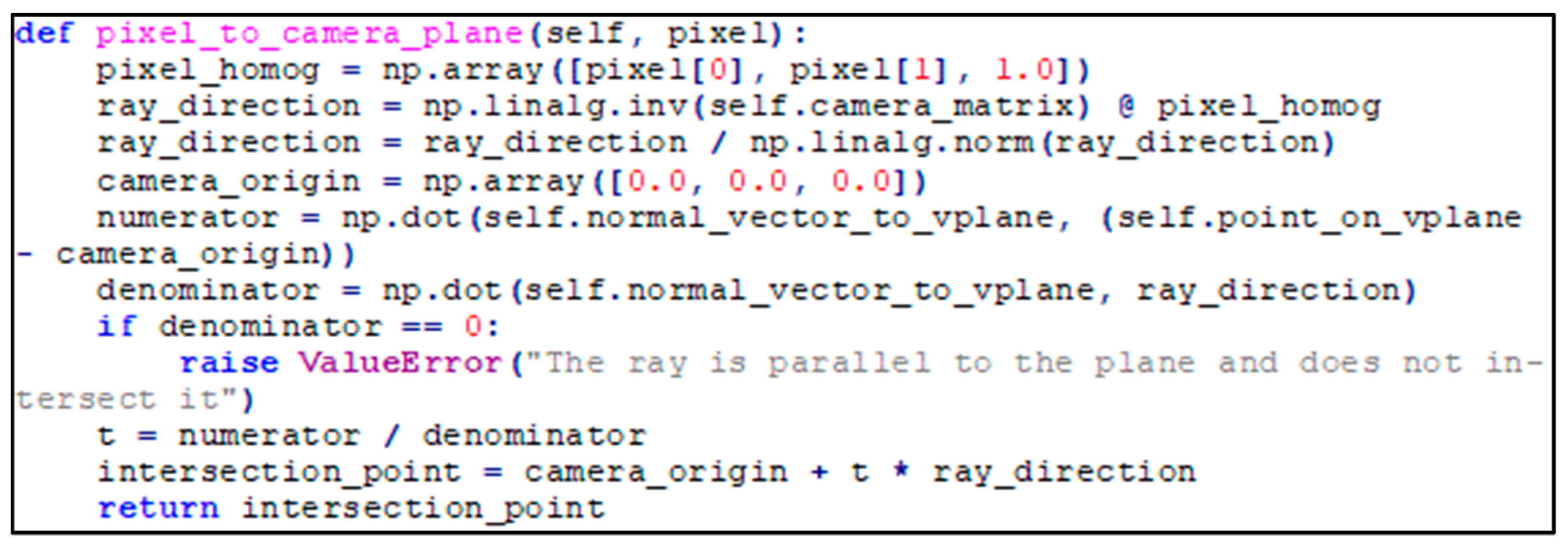
The Python function code implementing the calculations shown in the equations above is presented below [Figure 14].

In order to achieve accurate position estimation using the mentioned method, an additional issue had to be considered: the discrepancy in depth between the objects and the calibration chessboard. Since the camera was unable to directly measure the depth dimension of objects within its field of view, it was necessary to account for the fact that the detected object planes were elevated above the working field by an amount corresponding to their thickness. Assuming that the objects were produced with defined dimensions, the difference between the working plane and the objects’ planes was known for each shape. In the case under review, the calibration standard had a thickness of 10 mm, while all objects were 8 mm thick. The software compensated for this difference along the Z-axis by adjusting the robot’s observation position during the identification process, ensuring that the relationship between the TCP point and the object plane remained consistent with the relationship established during calibration relative to the virtual plane. For objects of varying thickness, it would have been possible to adjust the observation point by the corresponding difference along the Z-axis.

The final step in the position estimation process was to determine the pick point for the robot-mounted vacuum gripper using 2D images. In the analyzed thesis, all objects were designed to be grasped near their centers of gravity. Consequently, functions from the OpenCV library based on the computation of geometric moments were employed. The zero-order moment M₀₀, corresponding to the object’s area, along with the first-order moments M₁₀ and M₀₁, which represent the sums of the pixel coordinates, were used to calculate the coordinates of the object’s geometric center of gravity (c_x, c_γ) according to the Formula (12).

$${\mathrm{c}}_{\mathrm{x}}={\displaystyle \frac{{\mathrm{M}}_{10}}{{\mathrm{M}}_{00}}}, {\mathrm{c}}_{\mathrm{y}}={\displaystyle \frac{{\mathrm{M}}_{01}}{{\mathrm{M}}_{00}}}$$

(12)

In addition, to determine the object’s orientation relative to the reference system, the relationships between the central moments were utilized. The object’s rotation was computed from the second-order central moments μ₂₀, μ₀₂, and μ₁₁. The rotation angle θ was calculated as follows (13).

$$\mathsf{\theta }={\displaystyle \frac{1}{2}}\mathit{arctan}\left({\displaystyle \frac{2{\mathsf{\mu }}_{11}}{{\mathsf{\mu }}_{20}-{\mathsf{\mu }}_{02}}}\right)$$

(13)

Formula (13), derived from the analysis of the object’s moments with respect to its principal axes, provided the angle at which the object was oriented relative to the coordinate system. This information enabled the adjustment of the gripper to the object’s orientation, ensuring that parts were picked up in repeatable positions and precisely stacked in their designated locations.

4. Experiments and Results

This chapter presents an analysis of the results obtained from a series of measurements conducted to evaluate the performance of the implemented vision system, incorporating all proposed algorithms. The assessment of system performance was divided into two key areas: the accuracy of object identification algorithms and the overall efficiency of the sorting process based on the applied strategy. The first aspect focused on the correctness of object classification using identification methods such as the multilayer perceptron classifier, contour matching, and feature descriptors. The second aspect examined the effectiveness of the vision system in controlling the execution arm of the UR collaborative robot during the sorting task.

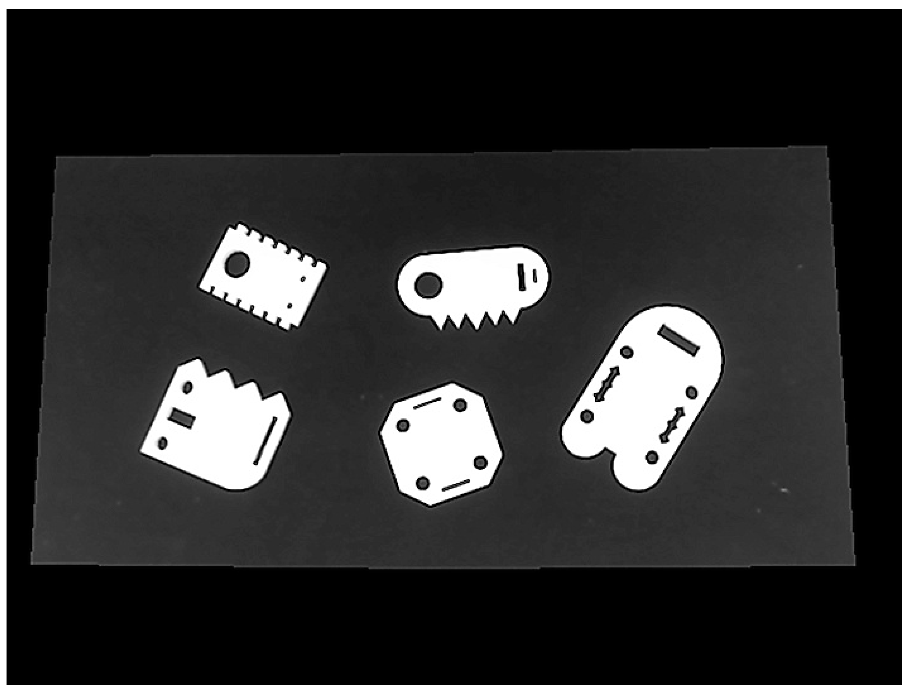
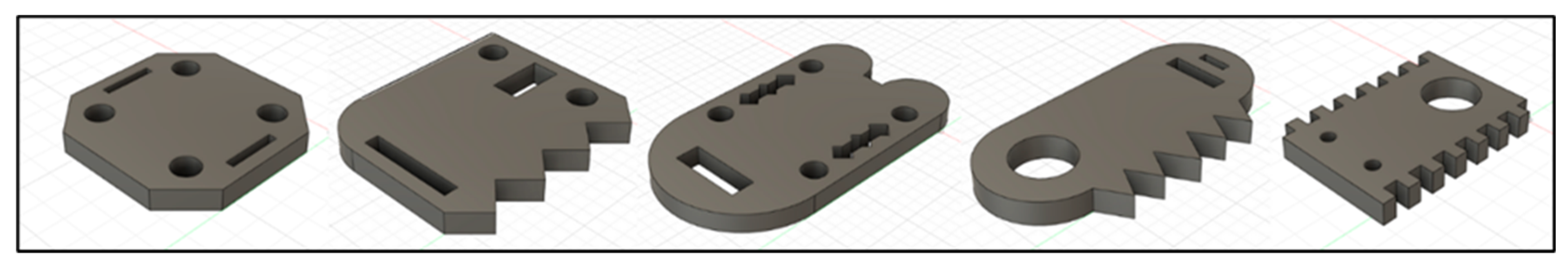
For the measurement process, five uniquely shaped objects [Figure 15], designed independently of specific production details, were fabricated using 3D printing technology. All parts were designed with a depth dimension “z” of 8 mm, and their “x” and “y” dimensions ranged from 50 to 120 mm. The diameters of round holes ranged from 5 to 20 mm, and those of other shapes ranged from 5 to 40 mm. The first stage of the experiment involved capturing 100 images using a webcam positioned on the robot’s flange at a predefined observation point relative to the workspace. All images were taken under consistent lighting conditions and identical system configurations. One sample of each of the five shapes was randomly placed in varying positions and orientations across consecutive images. The identification algorithms analyzed each image, and the correctness of label assignments was manually verified. A classification was considered correct if the assigned label corresponded to the object’s actual identity, whereas a misclassification occurred if an incorrect label was assigned.

To systematically assess classification performance, four states were defined for a given object label X:

• True Positive (TP): the object belonging to label X was correctly classified as X.
• False Positive (FP): the object belonging to label X was incorrectly classified as a different label.
• False Negative (FN): an object not belonging to label X was incorrectly classified as X.
• True Negative (TN): an object not belonging to label X was correctly classified as a different label.

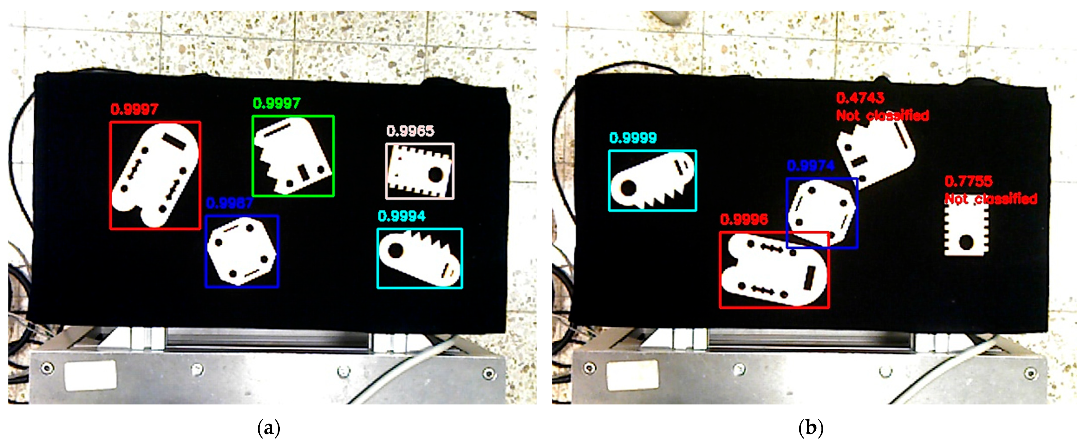
The identification algorithm using multilayer perceptrons (described in greater detail in Section 3) was the first to be tested. This algorithm detected shape contours and classified them based on a pre-trained model. A confidence threshold of 96% was set; objects below this threshold were considered unclassified.

To visualize the results, each object was assigned a specific color outlining its detected contour [Figure 16], along with a match probability [Figure 17]. If an object was not classified, this information was explicitly indicated, and its detected contour was marked accordingly. The absence of any contour labeling in the visualization signified a failure in the contour detection stage. The neural network-based identification achieved high accuracy in both contour detection and classification.

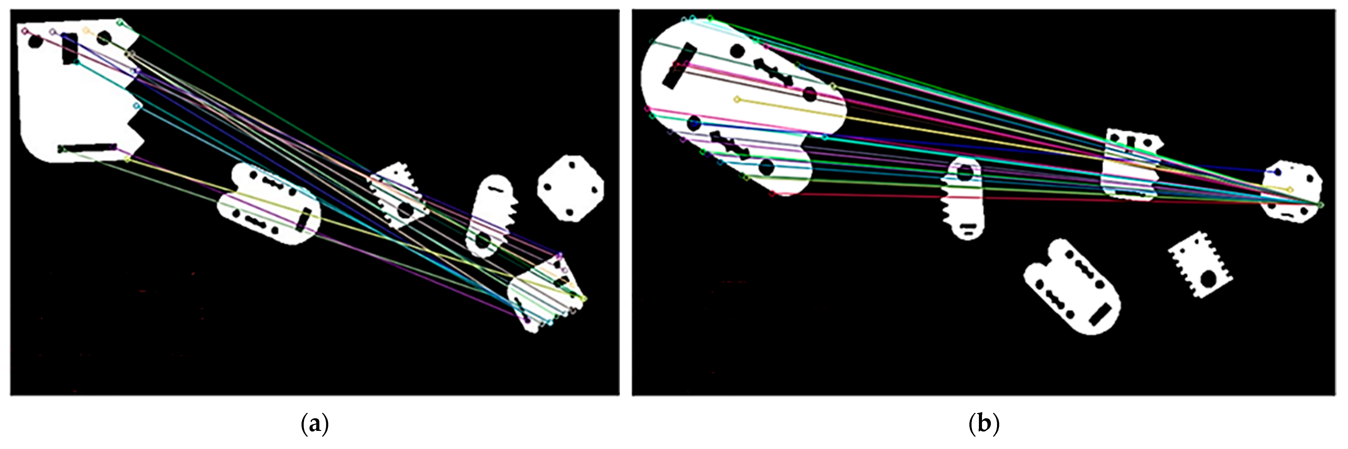
The next tested method utilized feature descriptor matching for object identification (described in Section 3). This algorithm detected object contours within the workspace and compared them to a reference image of one of the shapes, marking contours that exhibited a sufficient number of matching descriptors. A minimum threshold of 10 descriptor matches with a ratio value of at least 0.55 was established. As with the MLP classifier, the algorithm’s performance was assessed based on the correct identification of five distinct objects across all test images [Figure 18].

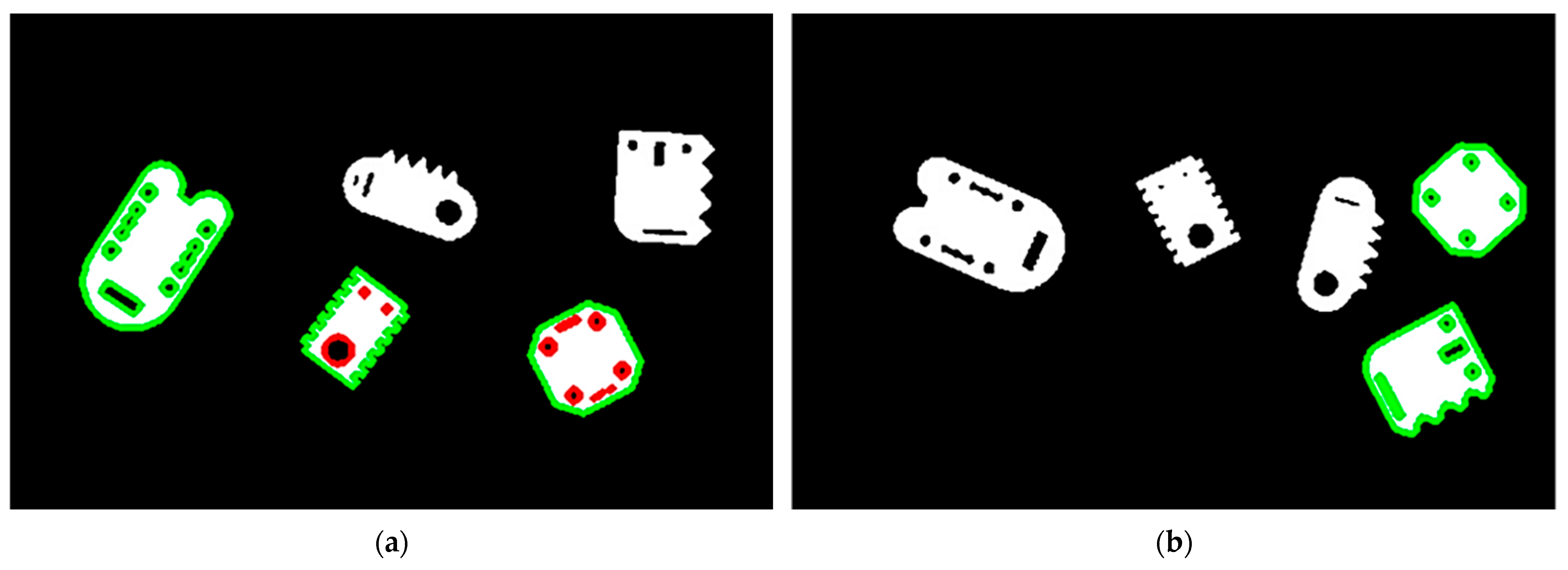
The last tested method was an approach that involved contour-based identification, in which detected contours were matched to reference contours (described in Section 3). A single reference image was selected for each shape, and objects in the test images were compared against these references. Contours with sufficiently similar parameters were identified using a hierarchical detection algorithm, which first analyzed external contours relative to the reference shape. Three different contour matching methods were employed, and their arithmetic mean was computed to determine the final match. For contours that satisfied the external matching criteria, an additional internal contour analysis was conducted to verify whether the number and shape of internal contours corresponded to the reference object.

A color-coded visualization scheme [Figure 19] was used to represent the identification results. Contours classified as correctly matched were highlighted in green, while internal contours that exhibited incorrect numbers or mismatched shapes were marked in red. Fully identified objects had all contours displayed in green. Objects with red-marked contours failed the internal contour analysis, whereas those without any marked contours had already been rejected at the external contour detection stage.

The results of all tests for all the identification methods were collected to compare the effectiveness of the methods. The following table [

Table 3. Summary of occurrence counts for identification categories for each method.

Occurrence		Value
		Object No. 1	Object No. 2	Object No. 3	Object No. 4	Object No. 5	Overall
True positive [TP]	MLP classifier	87	83	98	74	77	419
	feature descriptor	13	65	76	56	65	275
	contour similarity	3	91	98	21	69	282
False positive [FP]	MLP classifier	13	17	2	26	23	81
	feature descriptor	87	35	24	44	35	225
	contour similarity	97	9	2	79	31	218
False negative [FN]	MLP classifier	0	5	8	0	2	15
	feature descriptor	3	15	123	7	46	194
	contour similarity	1	24	7	0	0	32
True negative [TN]	MLP classifier	400	395	392	400	398	1985
	feature descriptor	397	385	277	393	354	1806
	contour similarity	399	376	393	400	400	1968

] collects the results of all identification methods achieved in the categories true positive, false positive, false negative, and true negative, with a distinction by method.

To facilitate a comparative analysis of the identification methods, performance metrics were derived from experimental data. The evaluation was based on four key indicators: sensitivity, specificity, precision, and accuracy, calculated according to the following formulas.

• Sensitivity, determined by the Formula (14),

$${\displaystyle \frac{TP}{TP+FN}}$$

(14)

• Specificity, determined by the Formula (15),

$${\displaystyle \frac{TN}{TN+FP}}$$

(15)

• Precision, determined by the Formula (16),

$${\displaystyle \frac{TP}{TP+FP}}$$

(16)

• Accuracy, determined by the Formula (17),

$${\displaystyle \frac{TP+TN}{TP+TN+FP+FN}}$$

(17)

A summary of the results achieved for the above key indicators is presented in

Table 4. Summary of effectiveness results achieved for each method.

Benchmark		Value
		Object No. 1	Object No. 2	Object No. 3	Object No. 4	Object No. 5	Overall
Sensitivity [%]	MLP classifier	100	94	92	100	97	96.5
	feature descriptor	80	91	51	75	54	58.6
	contour similarity	75	79	93	100	100	89.8
Specificity [%]	MLP classifier	97	96	99	94	95	96.1
	feature descriptor	96	95	88	95	88	88.9
	contour similarity	80	98	99	84	93	90.0
Precision [%]	MLP classifier	87	83	98	74	77	83.8
	feature descriptor	84	79	52	82	53	55.0
	contour similarity	03	91	98	21	69	56.4
Accuracy [%]	MLP classifier	97	96	98	95	95	96.2
	feature descriptor	92	94	81	91	81	83.2
	contour similarity	80	93	98	84	94	90.0

.

Additionally, the F1-score was computed for each method (

Table 5. Summary of all key indicators achieved for each identification method.

Identification Method	Sensitivity	Specificity	Precision	Accuracy	F1-Score
MLP classifier [%]	96.5	96.1	83.8	96.2	89.7
feature descriptor [%]	58.6	88.9	55.0	83.2	56.7
contour similarity [%]	89.8	90.0	56.4	90.0	69.3

). This metric provides a balanced measure of model performance by considering both precision and sensitivity. It is particularly useful in evaluating the performance of classification models when it is important to balance indicators that indicate misidentifications and omissions. The F1-score value is calculated as a harmonic average of precision and sensitivity, allowing meaningful comparison of models. For each of the analyzed methods, the F1-score value was determined according to the Formula (18).

$$F_1=\left({\displaystyle \frac{2}{{sensitivity}^{-1}+{precision }^{-1}}}\right)=2·{\displaystyle \frac{precision ·sensitivity}{precision+sensitivity}}$$

(18)

The results indicate that the MLP classifier demonstrated the highest overall performance, achieving a strong balance between sensitivity and precision. A significant portion of false positives resulted from classification scores falling just below the 96% confidence threshold. False negatives, where an object was incorrectly assigned to another shape, were observed in only a small number of cases. The contour similarity method showed competitive sensitivity but lower precision, while the feature descriptor approach exhibited the lowest accuracy among the tested methods [Figure 20].

In the second testing phase, the performance of the object sorting algorithm—implemented with a vision system and a UR cobot arm—was evaluated using three selection strategies. For each strategy, ten objects (two copies per shape) were placed on the workspace, and the algorithm was required to accurately identify and sort them. A series of measurement cycles was conducted to ensure reliable results.

For the random selection strategy, the algorithm selected objects solely based on the highest matching coefficient to the reference pattern without following any predetermined order. The ordered selection strategy enforced a sequential approach, where the algorithm processed objects with label no. 1 first, then label no. 2, and so on. In the label-specific selection strategy, the algorithm manipulated only objects of a defined shape while ignoring the others.

Overall, the analysis of the sorting algorithm revealed that its efficiency remained consistent across all selection strategies, with accuracy rates ranging from 85% to 95%. The performance issues were primarily attributed to the limitations of the object identification process. The random selection strategy provided a slight advantage by allowing the algorithm to choose the object that best met the identification criteria, thereby increasing the likelihood of successful identification and sorting. The differences in performance among the strategies were minimal, indicating that the overall sorting efficiency was heavily dependent on the underlying effectiveness of the identification process. Thus, optimizing the object identification stage was essential for enhancing the system’s overall performance.

5. Conclusions

The research described the development of a vision system integrated with a UR5 cobot, employing a multilayer perceptron neural network for object classification and sorting and its comparison with conventional identification methods like contour similarity and feature descriptor matching. The objective was to develop and set up an automated robotic sorting station that relied solely on images captured from a 2D webcam mounted on the cobot’s flange. The goal was the detection, classification, localization in 3D space, and manipulation of objects within the cobot’s workspace, all based on image analysis and recognition.

The vision system was designed for object sorting based on shape recognition and was integrated with the Universal Robots UR5 cobot. The software was developed using the Python 3.12 programming environment, utilizing essential libraries such as OpenCV (version 4.10.0.84), NumPy (version 1.26.4), and scikit-learn (version 1.5.0). Communication between the vision system and the cobot was facilitated via the TCP/IP protocol, with movement commands transmitted as data frames enabled by a custom-made framework on the Polyscope software platform. A key element of the system was the calibration process, which was performed in a hand-in-eye configuration. This process established the spatial relationship between the camera and the cobot and enabled the determination of a virtual plane parallel to the workspace—crucial for calculating object positions in 3D space.

The study provided an in-depth analysis of various object identification methods tailored to the specific use case. Classical image analysis techniques were examined, including contour similarity based on Hu moments and feature descriptor matching using SIFT with FLANN-based matching. Performance measures were determined both for the object identification algorithms and to assess the overall efficiency of the sorting process depending on the applied strategy. Functional tests during the verification phase involved the evaluation of a confusion matrix across five key performance metrics: sensitivity, specificity, precision, accuracy, and the F1-score. The results demonstrated that the neural network-based identification method outperformed classical methods in all categories—for example, achieving 96.2% accuracy for the MLP classifier compared with 90% for contour similarity and 83.2% for feature descriptor matching—while also offering greater simplicity in implementation. The MLP classifier showed very high performance in terms of sensitivity, specificity, and accuracy (all approximately 96%), with only slightly lower performance in precision (83.8%), whereas the other methods often exhibited precision levels in the 50–60% range. Moreover, the F1-score, which is particularly useful in evaluating the balance between misidentifications and omissions, further underscored the superiority of the MLP classifier by achieving nearly 90% (89.7%), significantly outperforming the alternative methods. By employing widely available tools for model training, the system achieved competitive performance without requiring extensive expertise in computer vision or neural network modeling. The resulting neural network model provided satisfactory results, effectively competing with traditional vision methods. Additionally, the developed system showcased the potential for deploying machine learning techniques to build robust and flexible industrial vision systems. This approach allowed for model training by simply importing a reference dataset rather than necessitating a complete analysis from scratch by a qualified engineering team. Consequently, the method significantly reduced the complexity and time required for vision system development, thereby promoting the adoption of intelligent automation in industrial environments.

Furthermore, the system demonstrated its flexibility by incorporating various object selection strategies to optimize the sorting process. The differences in performance among these strategies were minimal; this observation underscored that the overall efficiency of the sorting process was heavily dependent on the underlying effectiveness of the object identification stage.

Overall, the project successfully validated the concept of a vision-based sorting system for a collaborative robot. The innovative integration of AI-driven techniques with conventional image processing methods aligns with the principles of Industry 4.0, where industrial processes increasingly integrate advanced algorithms and multidisciplinary scientific solutions. The developed system highlights the potential for deploying machine learning techniques to build robust and flexible industrial vision systems that can be trained by simply importing a reference dataset rather than having the problem analyzed from scratch. This approach significantly reduces the complexity and development time of vision systems, thereby facilitating the adoption of intelligent automation in industrial environments.