Trustworthy Load Prediction for Cantilever Roadheader Robot Without Imputation

Abstract

We propose a trustworthy load prediction method for a cantilever roadheader robot without imputation. Specifically, we design a load-trustworthy-boosting (LTB) algorithm for coal and rock cutting loads that accounts for missing data in complex underground environments. We introduce a trustworthy decision tree that integrates mixed-integer programming (MIP) and Missing Incorporated in Attributes (MIA) as the base predictor, which can handle missing data, thereby accelerating load prediction and improving prediction accuracy. Furthermore, we utilize boosting techniques to enhance the prediction performance of the base predictor by incorporating cutting safety–trust constraints during the prediction process. We derive the convergence of the algorithm theoretically and verify the accuracy and reliability of the algorithm through experiments. The experimental results show that the proposed algorithm is superior to state-of-the-art load prediction algorithms both without and with missing data considered. This method can provide a reliable decision-making basis for underground unmanned intelligent excavation.

1. Introduction

The increasing integration of robotics in underground coal mining has raised critical challenges related to trustworthy decision-making and data integrity. Recent advances in intelligent control have made data-driven load prediction essential for cantilever roadheader robots. However, underground environments are often characterized by incomplete, noisy, and inconsistent sensor data, thus posing significant reliability risks to conventional prediction models [1,2].

The cantilever roadheader robot is an indispensable piece of equipment for coal mining, with intelligent and precise cutting serving as a prerequisite for automated tunneling with minimal human intervention [3,4]. Currently, the progress in unmanned and intelligent mining remains slow, primarily due to difficulties in obtaining information on coal–rock characteristics, equipment status, and working conditions in harsh mining environments [5,6,7,8]. As a consequence, many existing operations use simplistic criteria for detecting changes in cutting conditions, and load identification models that consider complex and variable environments are lacking. These gaps make it difficult to design effective cutting control methods [9,10].

Multi-sensor information fusion has been widely applied in fields such as intelligent vehicles, industrial robotics, disaster early warning, and autonomous driving  [11,12,13,14,15,16]. In the mining industry, multi-sensor techniques have been introduced for coal–rock state identification, remote monitoring, and fault diagnosis—particularly for shearers [17,18]. The research on multi-sensor fusion for roadheaders began more recently, focusing on dynamic load identification and equipment diagnostics. For instance, artificial neural networks have been used to recognize the cutting state of a roadheader and improve cutting performance via multi-parameter evaluation (e.g., accounting for rock properties) [19]. Similarly, multiple neural networks combined with evidence theory have been employed to integrate cutting current, vibration, and pressure signals, significantly enhancing the reliability of load identification [20]. These studies demonstrate that leveraging multiple sensor signals can improve the accuracy and reliability of coal–rock load predictions.

However, real-world underground conditions pose additional challenges. High-quality unmanned tunneling demands improved efficiency, assured roadway quality, and reliable safety controls. In practice, factors such as sensor interference or harsh environmental conditions often result in missing sensor data [21,22]. For example, during  operation, measurements from the lifting or rotary cylinder pressure sensors or the vibration accelerometer may be missing, which can lead to misjudgments of the cutting state. Most current methods either discard data entries with missing values or fill them via imputation, but both approaches can reduce prediction accuracy and compromise the safety and reliability of the cutting process [23]. The traditional approaches to load prediction typically rely on data imputation techniques to handle missing inputs. These methods often introduce estimation biases and degrade the robustness of predictive models. More critically, they fail to address the uncertainty and trustworthiness of such reconstructed data.

Given these shortcomings, we draw inspiration from the Missing Incorporated in Attributes approach proposed by Twala [24] and fairness-oriented decision tree optimization by Jeong et al. [25]. Building on these ideas, we develop a new ensemble framework for load prediction. In particular, we propose a novel load-trustworthy-boosting (LTB) algorithm that uses a trustworthy decision tree (capable of handling missing data) as its base predictor, incorporating cutting safety constraints into the boosting process to ensure reliability.

Overall, this study contributes to the literature by removing the dependence on unreliable imputation procedures and introducing a principled trust modeling mechanism into the predictive modeling of mining robotics. This research lays the groundwork for safer and more autonomous intelligent excavation systems.

The main contributions of this paper are summarized as follows:

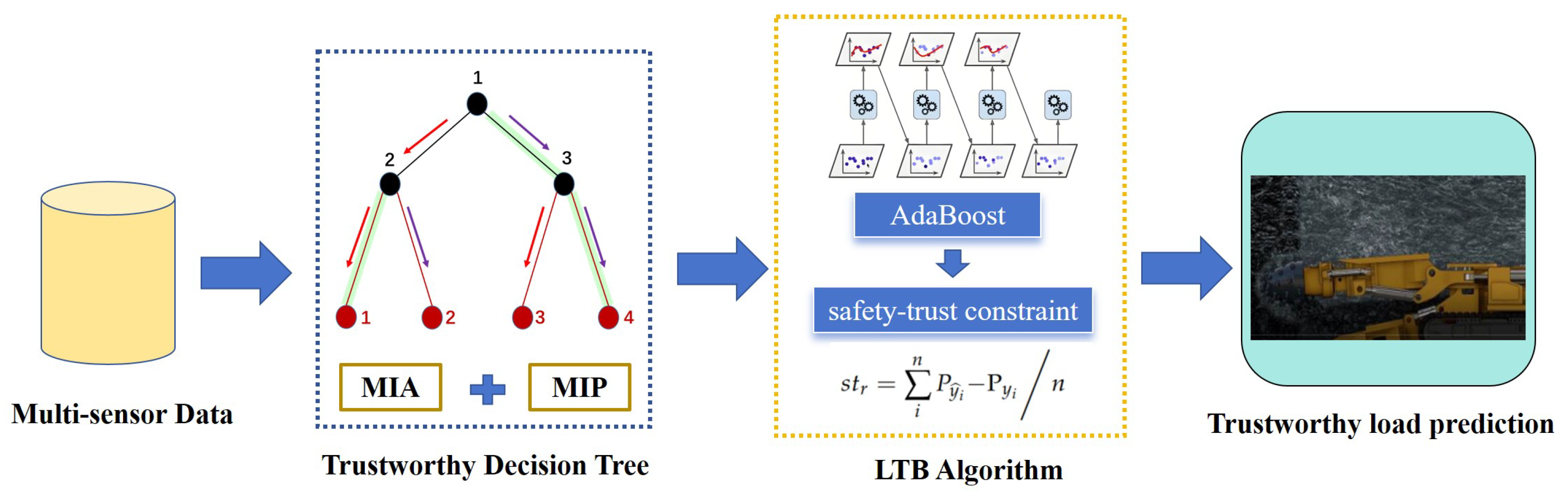
• We propose a load-trustworthy-boosting (LTB) framework that integrates safety constraints and missing data handling into a boosting-based load prediction model for underground tunneling.
• We develop a Trust MIP Tree as the base learner, combining MIA-based splitting with mixed-integer programming to directly encode cutting safety constraints during tree construction.
• We validate the proposed method using real-world underground multi-sensor datasets, demonstrating superior accuracy and robustness over classical models, even with 3% missing data.

The structure of this paper is as follows. Section 2 describes the experimental design for collecting key sensor information on cutting load, analyzes the underground data, and examines the impact of missing data on load prediction—providing a foundation for reliable load prediction in real conditions. Section 3 elaborates on the principles and procedures of the proposed LTB algorithm, including a theoretical convergence analysis. Section 4 presents a validation experiment using the collected real data and provides a detailed comparative analysis of the results with the current mainstream load prediction algorithms. Finally, Section 5 concludes the paper and outlines future research directions.

2. Collection and Analysis of Key Sensor Data for Cutting Load

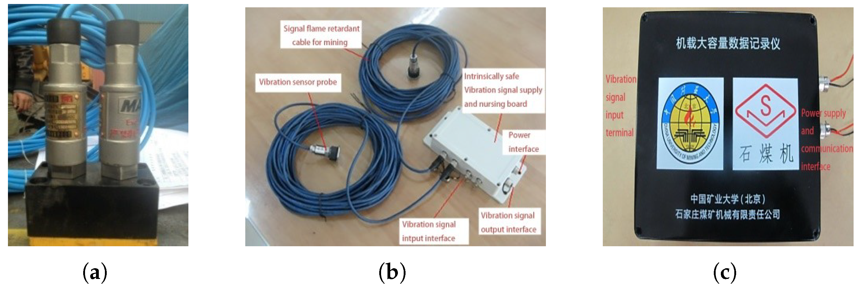
2.1. Data Acquisition Scheme

The working environment of a roadheader in underground coal mines is located 300 to 1000 m below the surface, with extremely harsh mining conditions, as shown in Figure 1. Due to these challenging conditions, load information cannot be obtained directly. For instance, directly measuring the cutting head load by installing a force measurement device on the cutting head is currently not feasible.

As shown in Figure 1, the working environment of the underground coal mine face is harsh, with complex geological conditions, making it difficult for single-sensor data to fully characterize changes in coal–rock conditions during the roadheader’s cutting process, and thus preventing accurate determination of cutting load changes. Based on actual field research and analysis of sensor data during the cutting process, as reported in the related literature [26,27], the key sensor data for cutting load identification primarily include cutting motor current, cutting cylinder pressure, and cutting arm vibration acceleration.

By installing detection sensors on the roadheader, a multi-sensor data collection experiment was conducted on the cantilever roadheader underground. The experimental model used was the EBZ-160 cantilever roadheader. In the experiment, a BYD-60 explosion-proof pressure transmitter, which meets coal mine safety standards, was used to measure the pressure of the cutting arm drive cylinder. An intrinsically safe GBC1000 acceleration sensor, independently developed by the laboratory, was used to measure the vibration acceleration of the cutting arm. The cutting motor current data were collected by the current sensor equipped on the machine. Additionally, the laboratory independently developed an onboard large-capacity data recorder (black box) for the roadheader, where all collected data were stored. The experimental equipment is shown in Figure 2. The experimental model operated for two weeks under normal conditions in an underground coal mine roadway, collecting a substantial amount of multi-sensor data, providing a rich and effective dataset for precise cutting load identification.

2.2. Data Analysis

After multiple complete work cycles, a substantial amount of multi-sensor underground cutting data were collected. The datasets from different working conditions accurately reflect the cutting state of the roadheader, providing a data foundation for identifying coal–rock cutting loads and enabling intelligent control. Some of the experimental data are shown in

Table 1. Partial experimental data.

Sample Sequence Number	Cutting Motor Current I/A	Rotary Cylinder Pressure ${\mathit{p}}_1/$MPa	Lifting Cylinder Pressure ${\mathit{p}}_2/$MPa	Vibration Acceleration of Cutting Arm Acc/m·s−2
1	100.21	18.15	19.83	4.53
2	26.03	6.13	6.54	0.81
3	53.24	6.68	7.12	0.92
4	82.12	14.95	16.15	3.05
5	114.16	18.32	20.15	6.13

.

A complete cutting work cycle of the roadheader typically consists of four processes: slotting, bottom-up cutting, floor cleaning, and side brushing. Representative data from each process were extracted to analyze the multi-sensor datasets. The data analysis excluded missing data, selecting only complete datasets that represent load variations under different working conditions. The analysis indicated that the multi-sensor data from underground cutting systematically change with different cutting conditions. The trends of multi-sensor datasets and coal–rock cutting loads under varying cutting conditions are shown in Figure 3.

2.3. Impact of Missing Data on Cutting Load Prediction

Missing data is a common challenge in practical engineering applications. When sensor data includes varying degrees of missing values, the approach used to address these gaps significantly impacts both the accuracy of predictive models and safety outcomes. Methods for addressing missing values have a long history in statistics [28,29,30,31,32]. Common imputation techniques involve replacing missing entries with new values, such as inserting dummy values, mean imputation, or regression imputation (e.g., k-NN regression) [33,34]. Multiple imputation is also widely used, drawing a set of possible values to fill missing entries rather than relying on a single replacement [35]. However, these methods separate missing data handling from model training, which can lead to incomplete information and introduce new biases, resulting in unreliable predictions in practical applications. Moreover, few studies have explored the impact of missing data on intelligent decision-making in coal mining. Many assume complete datasets or simply discard incomplete entries, which significantly reduces decision accuracy and poses serious safety risks. Therefore, this paper proposes a coal–rock cutting load prediction algorithm for roadheaders that is resilient to missing data, enhancing the reliability and safety of predictions through the introduction of safety–trust constraints.

3. Design of Load Prediction Algorithm

In this section, we propose the load-trustworthy-boosting (LTB) algorithm, which integrates multisource cutting sensor data with coal mining safety constraints to enable reliable and interpretable load prediction. The overall workflow of the proposed method is illustrated in Figure 4. The algorithm design is partially inspired by Jeong et al.’s research on fairness-aware machine learning [25]. Specifically, the LTB algorithm adopts the Trust MIP Tree as the base predictor, where the tree construction incorporates missing data through the Missing Incorporated in Attributes (MIA) strategy and optimizes decision splits using mixed-integer programming (MIP). On top of this, an AdaBoost-based ensemble learning module is employed to iteratively refine the base predictors. By tuning the associated hyperparameters, the algorithm balances prediction accuracy with safety–trust constraints, ensuring that load estimates remain both precise and compliant with operational safety requirements.

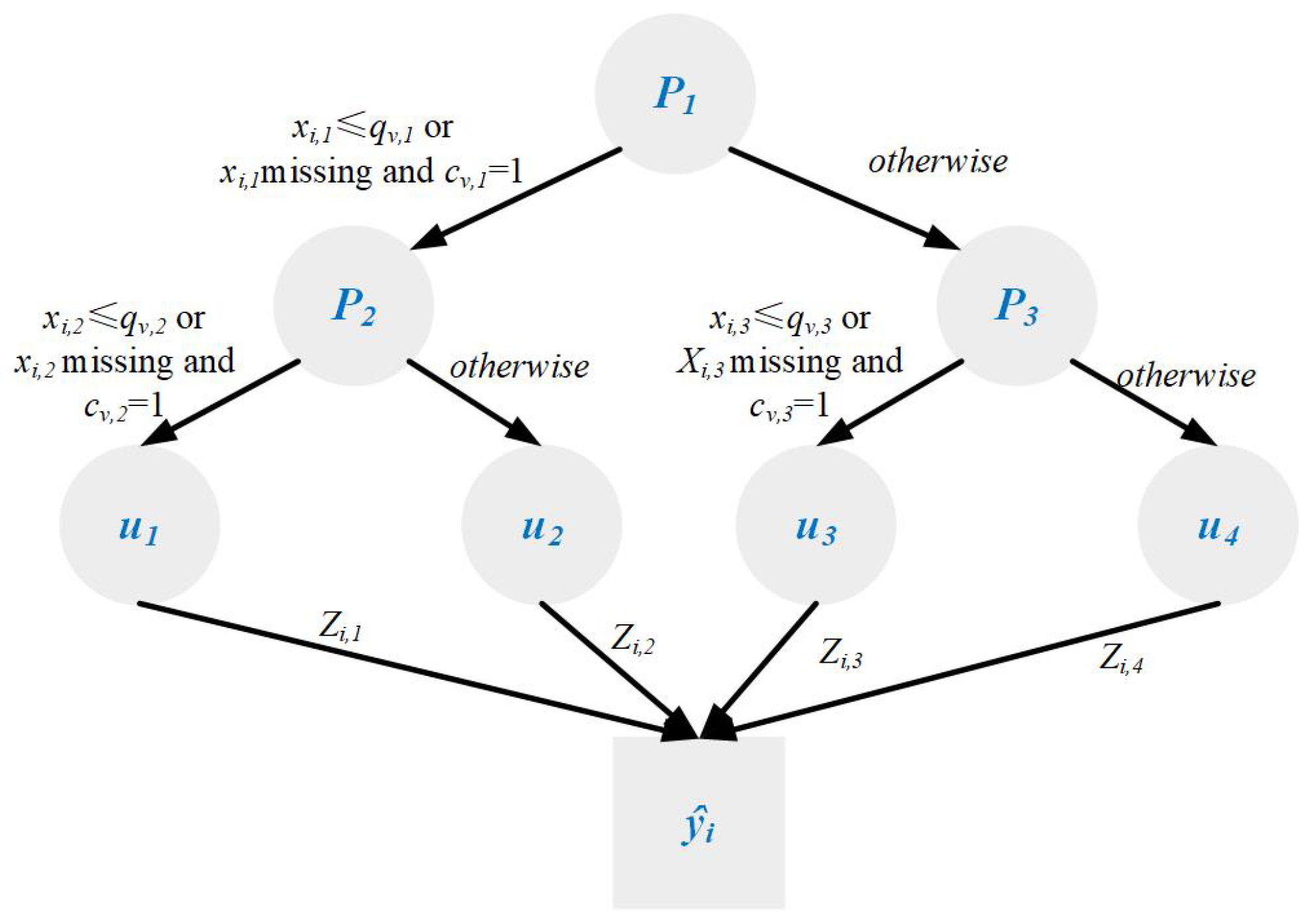
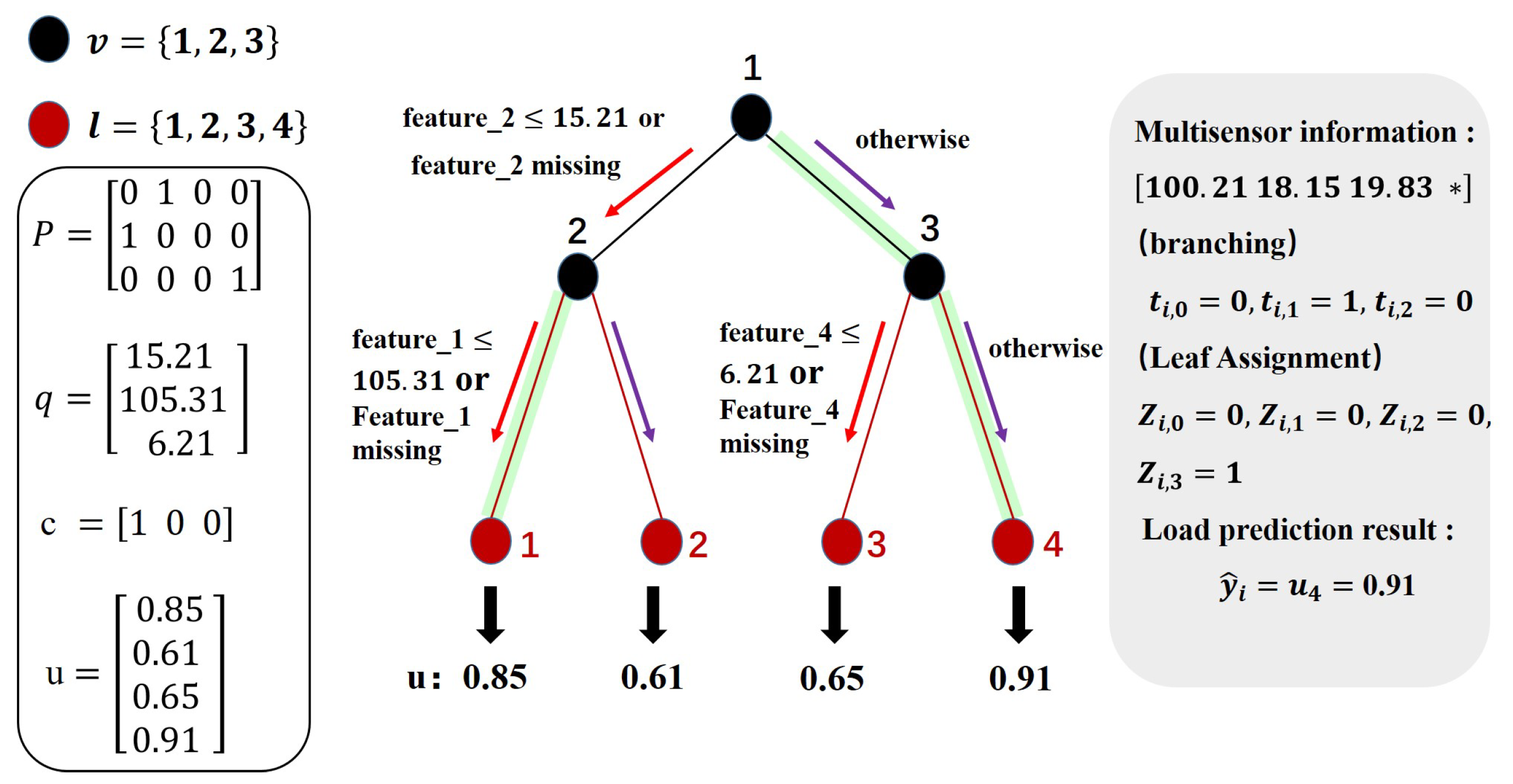
3.1. Trustworthy Decision Tree as a Base Predictor

Designing a reliable algorithm that accurately predicts changes in cutting load is essential for ensuring the safety and precision of intelligent tunneling. The current methods fail to account for the characteristics of incomplete and partially missing underground data, which increases production risks. Additionally, as mining depth and the complexity of cutting conditions grow, misjudging the load may lead to serious underground accidents. To address these challenges, this subsection proposes the Trust MIP Tree—a trustworthy decision tree capable of handling missing data—to serve as the base predictor for preliminary load identification. The Trust MIP Tree is a decision tree architecture designed to operate effectively on incomplete data without requiring imputation. It combines two key mechanisms:

• Multi-Path Information Aggregation (MIA): This mechanism allows the model to split samples with missing values along multiple valid paths, thereby preserving decision diversity and avoiding data discards.
• Trust-Aware Multi-Instance Prediction (MIP): In cases where multiple candidate paths are taken, MIP uses trust-weighted aggregation to generate a robust final prediction. This trust score reflects data completeness and consistency.

Specifically, Trust MIP Tree is a predictor that integrates the concepts of Missing Incorporated in Attributes (MIA) and mixed-integer programming (MIP). MIA incorporates missing values as split criteria within the decision tree, forming a distinct category that ensures load prediction remains robust despite missing data, thereby reducing the risk of misjudgment. Meanwhile, MIP is employed during the training of the fair decision tree to accelerate the predictor’s processing of missing values. Symbols and formulas related to MIP are detailed in the work of Jeong, Aghaei, et al. [25]. The approach used by the Trust MIP Tree to handle missing sensor data for load identification is illustrated in Figure 5.

We use a Trust MIP Tree with a depth of 2 as an example. A decision tree incorporating missing sensor data primarily involves four variables: P, q, c, and u. Specifically, q represents the sensor feature to be split, P denotes the split threshold at a decision tree branch node, c determines whether missing sensor data should be directed to the left or right at the branch node, and u represents the load prediction value at each leaf node. Finally, ${\widehat{y}}_i$ denotes the predicted load output.

Suppose there are n samples in the training dataset collected from underground sensors, where d represents the number of sensor features, v represents a branch node, and l represents a leaf node. For the i-th sensor sample $x_{i,j}$, where j is the feature at node v, if there is no missing value for feature $P_j$, the branch splits based on the threshold q. Specifically, if x_i,j ≤ q_v, the sample is split to the left; if x_i,j > q_v, it is split to the right. If the value $x_{i,j}$ is missing for feature $P_j$, the branch splits based on the value $c_v$ at the node. If $c_v$ = 1, the sample is assigned to the left; if $c_v$ = 0, it is assigned to the right.

Finally, a prediction is conducted for all data points reaching the same leaf node. For leaf node l, the final load prediction value is $u_l\in {\hat{y}}_i$. To determine how to select the output $y_i$ based on input values, we adopted Jeong’s method [25]. For any sample ($x_i$, $y_i$), a one-hot-encoded value $Z_i$ is calculated; if $Z_{i,l}$ = 1, it indicates that the data point reaches leaf node l and assigns ${\widehat{y}}_i$ = $u_l$. Figure 6 illustrates the load prediction process using actual underground sensor data.

The Trust MIP Tree treats missing values as a distinct category of sensor data and, at each branch node, splits features to the left or right based on whether the data is missing. As illustrated in Figure 6, v represents a branch node, and l represents a leaf node. P denotes the underground sensor feature to be split, q is the actual split threshold used in traditional decision trees, and c indicates whether missing values are directed to the left or right. u represents the predicted load value. P is a $3\ast 4$ matrix, where each row specifies the sensor feature used for splitting at each branch node. The second element of the first row of P is 1, indicating that feature 2 is used for splitting at branch node 1. Similarly, feature 1 is used for splitting at branch node 2, and feature 4 is used for splitting at branch node 3.

On the right side of Figure 6, a data point from underground cutting sensor data is displayed, representing the cutting motor current, lifting cylinder pressure, rotary cylinder pressure, and cutting arm vibration acceleration, respectively. Two variables, $t_i$ and Z, are introduced to calculate split values at branch nodes and leaf nodes, respectively. $Z_i$ is a one-hot-encoded vector indicating the final predicted leaf node. At branch node 1, feature 2 has a value of 18.15, which splits to the right, assigning $t_{i,0}$ = 0. At branch node 2, feature 1 has a value of 100.21, which splits to the left, assigning $t_{i,1}$ = 1. At branch node 3, feature 4 is missing, which splits to the right, assigning $t_{i,2}$ = 0. The Z values are assigned according to the split sequence, resulting in a final load prediction output of ${\widehat{y}}_i$ = $u_4$ = 0.91. Notably, mixed-integer programming was used in the training of the Trust MIP Tree, which accelerates the handling of missing values. All prediction processes were completed using Gurobi software (9.1.1).

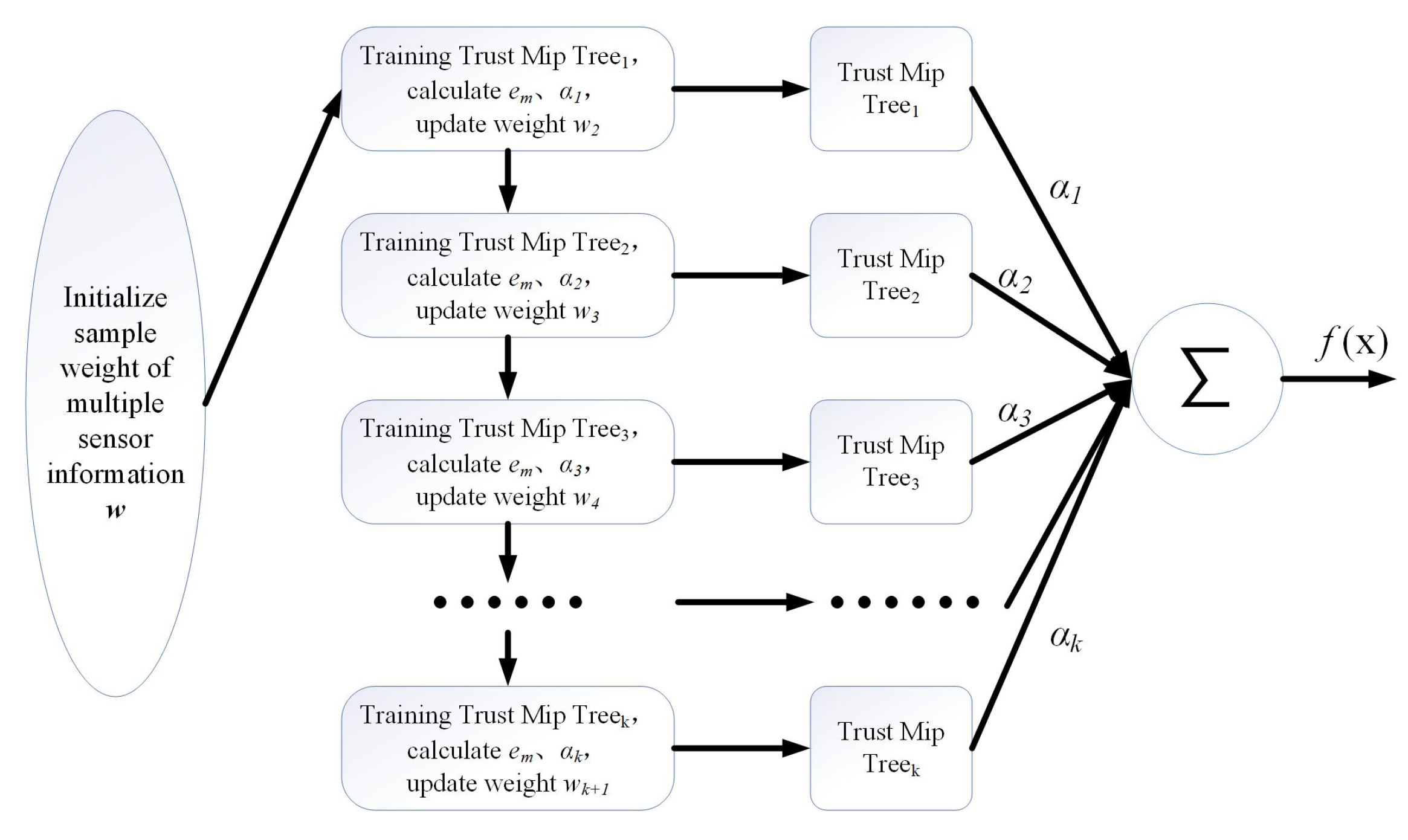
3.2. Load-Trustworthy-Boosting Algorithm (LTB)

AdaBoost is an enhanced classifier based on ensemble learning and has become one of the most effective methods for solving classification and prediction tasks. However, traditional AdaBoost methods primarily focus on prediction accuracy, often overlooking the safety and reliability requirements of practical applications. Therefore, we improved the AdaBoost algorithm and proposed a trustworthy predictive boosting ensemble algorithm (LTB) suitable for coal–rock load identification. The LTB algorithm utilizes the Trust MIP Tree, which can handle missing sensor data, as its base predictor. To further enhance the accuracy and reliability of the algorithm, we calculated the error rate of each base predictor using an ensemble approach and incorporated coal mining cutting safety–trust constraints into the error rate calculation. During the iteration process, we continuously updated the error rate to account for safety–trust constraints and assigned higher weights to misclassified samples. By calculating and updating the weight distribution of different sensor data in the base predictor, an optimal predictor meeting the constraints was obtained through iteration. The overall flowchart of LTB algorithm is shown in Figure 7.

In the algorithm design process, we first initialize the sample weights $w_i$ for each base predictor. After training the initial base predictor, its error rate is calculated. To enhance prediction accuracy and reliability, the overall prediction error rate $e_m$ of LTB algorithm consists of two components: the data sample error rate and the safety–trust constraint $s{t}_r$. This relationship can be expressed by the following formula:

$$e_r=\sum _{i=1}^n\left(w_i\ast \left|{\stackrel{\wedge }{y}}_i-y_i\right|\right)/\phantom{\sum _{i=1}^n\left(w_i*\left|{\stackrel{\wedge }{y}}_i-y_i\right|\right)\sum _{i=1}^n{w}_i}\sum _{i=1}^n{w}_i$$

(1)

$$e_m=e_r+u\ast s{t}_r$$

(2)

Here, u represents the weight of safety–trust constraint. By adjusting the value of u, balance between the algorithm’s accuracy and safety can be achieved. The selection of u is defined based on the cutting requirements under different scenarios. We refer to the China Coal Society group standard, “Classification, Grading Technical Conditions and Evaluation of Intelligent Coal Mines (Underground)” (T/CCS 001-2020), and use constant power cutting as the safety constraint indicator to find the optimal solution under safe cutting conditions:

$$mins{t}_r=P_{{\widehat{y}}_i}-{\mathrm{P}}_{y_i}s.t.s{t}_r\le c$$

(3)

The smaller the $s{t}_r$, the better the adaptability of the cutting pick to the load during the cutting process, resulting in greater cutting safety and efficiency. Different constraint indicators can be defined based on the specific working conditions of different mines. Here, we define the safety–trust constraint as follows:

$$s{t}_r=\sum _i^n{P}_{{\widehat{y}}_i}-{\mathrm{P}}_{y_i}/\phantom{\sum _i^n{P}_{{\widehat{y}}_i}-{\mathrm{P}}_{y_i}n}n$$

(4)

We draw on the traditional AdaBoost algorithm, utilizing a linear combination of base predictors to minimize the loss function of the LTB algorithm:

$$l_{exp}\left(h\right|D)=E_{x\sim D}[e^{-y_{\mathrm{i}}h\left(i\right)}+e^{-y_{i}h\left(i\right)}|s{t}_r]$$

(5)

Here, $h\left(i\right)$ represents the base predictor, which is the Trust MIP Tree. After training the initial base predictor, classifiers $h_k\left(i\right)$ and weight coefficients ${\alpha }_k$ are generated iteratively. A greedy algorithm is employed to update the weight ${\alpha }_k$ of each base predictor to minimize the loss function:

$$\begin{array}{c}{l}_{exp}\left({\alpha }_k{h}_k\right|D_k)=E_{x\sim D_k}[e^{-y_i{\alpha }_k{h}_k\left(i\right)}+\mu e^{-y_i{\alpha }_k{h}_k\left(i\right)}|s{t}_r]\\ =E_{x\sim D_k}[e^{-{\alpha }_k}\mathrm{I}(y_i=h_k\left(i\right))+e^{{\alpha }_k}\mathrm{I}(y_i\ne h_k\left(i\right))]\\ +\mu E_{x\sim D_k}\left[e^{-{\alpha }_k}(\mathrm{I}(y_i=h_k\left(i\right)|s{w}_r)+e^{{\alpha }_k}(\mathrm{I}(y_i\ne h_k\left(i\right)|s{t}_r)\right]\\ =e^{-{\alpha }_k}{P}_{x\sim D_k}\left[\mathrm{I}(y_i=h_k\left(i\right))+\mu \left(\mathrm{I}\right(y_i=h_k\left(i\right)|s{t}_r\right]\\ +e^{{\alpha }_k}{P}_{x\sim D_k}\left[\mathrm{I}(y_i\ne h_k\left(i\right))+\mu \left(\mathrm{I}\right(y_i\ne h_k\left(i\right)|s{t}_r\right]\\ =e^{-{\alpha }_k}(1-e_r-\mu s{t}_r)+e^{{\alpha }_k}(e_r+\mu s{t}_r)\\ =e^{-{\alpha }_k}(1-e_m)+e^{{\alpha }_k}\left(e_m\right)\end{array}$$

(6)

It is important to note that the correct prediction probability distribution encompasses both the sample probability of accurate load prediction and the probability of meeting safe cutting constraints, represented as $1-e_m$. Conversely, the incorrect prediction probability includes both the probability of incorrect prediction and the probability of failing to meet safety reliability, represented as $e_m$. Considering the derivative of the above loss function,

$${\displaystyle \frac{\partial l_{exp}\left({\alpha }_k{h}_k\right|D_k)}{\partial {\alpha }_k}}=-e^{-{\alpha }_k}(1-e_m)+e^{{\alpha }_k}\left(e_m\right)$$

(7)

By setting (7) to zero, the weight coefficient update formula for the LTB algorithm at the k-th base predictor is obtained as follows:

$${\alpha }_k={\displaystyle \frac{1}{2}}ln\left({\displaystyle \frac{1-e_m}{e_m}}\right)$$

(8)

According to (8), the sample distribution weight for the next predictor can be adjusted to increase the weight of samples in the base predictor. This adjustment improves the likelihood of correct predictions while reducing the risk of unsafe predictions:

$$w_{k,i}=w_{k-1,i}exp[{\alpha }_{k-1}\left|{\stackrel{\wedge }{y}}_i-y_i\right|]$$

(9)

After multiple iterations, the optimal LTB predictor is ultimately derived from (10):

$$f\left(x\right)={\sum }_{k=1}^k{\alpha }_k{\stackrel{\wedge }{y}}_i$$

(10)

The detailed implementation of LTB algorithm is provided in Algorithm 1.

Algorithm 1 The detailed implementation of the LTB algorithm.

LTB Algorithm Input: Dataset $D=\{(x_1,y_1),(x_2,y_2),\dots ,(x_n,y_n)\}$; $y_i\in Y$; base predictor $h\left(x\right)$; Number of iterations K. Process: 1: Initialize weight $w_i$ 2: for $k=1,2,\dots ,K$ do 3: Train predictor $h_k\left(x\right)$ based on weight Add safety-trust constraint to calculate total error rate $e_m=e_r+u\times s{t}_r$ 4: Update weight coefficient ${\alpha }_k={\displaystyle \frac{1}{2}}ln\left({\displaystyle \frac{1-e_m}{e_m}}\right)$ 5: Update sample distribution weights: $w_{k,i}=w_{k-1,i}exp\left[{\alpha }_{k-1}\left|\widehat{y_i}-y_i\right|\right]$ 6: end for Output: $f\left(x\right)={\sum }_{k=1}^K{\alpha }_k\widehat{y_i}$

From the above algorithm design steps, it is evident that the proposed LTB algorithm incorporates cutting safety–trust constraints during the weight updating process. This approach ensures prediction accuracy while considering the safety of the cutting process, thereby extending and enhancing the basic AdaBoost algorithm.

3.3. Convergence Analysis of LTB Algorithm

In traditional convergence analysis of AdaBoost algorithm, the derivation is usually based on a simple binary classification problem. To ensure rigor in the derivation process, we follow the traditional approach and make the following assumptions for the theoretical derivation of the LTB algorithm: the sensor information training set is denoted as D = (x₁,y₁), (x₂,x₁), …, (x_n,y_n), where $i=1,2,\dots ,n$; the output prediction is the normalized load $y_i\in Y=\left\{-1,1\right\}$, where −1 indicates a lower load, representing coal or softer material, and 1 indicates a higher load, representing hard rock; and the base predictor is a single Trust MIP Tree, denoted as h_k(x), which can handle missing features without affecting its performance. The sample weight of each base predictor is w_k(i), the weight update coefficient is ${\alpha }_k$, the iteration count is k, where j = 1, 2, …, k, and the sample normalization factor is Z. Then, the sample weight can be represented by the following formula:

$$w_{k+1}\left(i\right)=w_k\left(i\right)·{\displaystyle \frac{e^{-{\alpha }_k{y}_i{h}_k\left(i\right)}}{Z_k}}=···=w_1\left(i\right)·{\displaystyle \frac{e^{-y_i{\displaystyle \sum _{j=1}^k}{\alpha }_j{h}_j\left(i\right)}}{Z_1···Z_{k-1}{Z}_k}}$$

(11)

Let $\overrightarrow{\alpha }={\left[{\alpha }_1,{\alpha }_2,···,{\alpha }_k\right]}^k$, $\overrightarrow{h}\left(x\right)={\left[h_1,h_2,···,h_k\right]}^k$, and then (11) can be rearranged as follows:

$$w_{k+1}\left(i\right)=w_1\left(i\right)·{\displaystyle \frac{e^{-y_i〈\overrightarrow{\alpha },\overrightarrow{h}\left(i\right)〉}}{{\displaystyle \prod _{j=1}^k}{Z}_j}}={\displaystyle \frac{e^{-y_i〈\overrightarrow{\alpha },\overrightarrow{h}\left(i\right)〉}}{n{\displaystyle \prod _{j=1}^k}{Z}_j}}$$

(12)

Since the sum of all sample weights is 1, i.e., ${\displaystyle \sum _{i=1}^n}{w}_{k+1}\left(i\right)=1$, let $f\left(x_i\right)=〈\overrightarrow{\alpha },\overrightarrow{h}\left(i\right)〉$, and then (12) can be rearranged as follows:

$${\displaystyle \prod _{j=1}^k}{Z}_j={\displaystyle \frac{1}{n}}\sum _i{e}^{-y_i〈\overrightarrow{\alpha },\overrightarrow{h}\left(i\right)〉}={\displaystyle \frac{1}{n}}\sum _i{e}^{-y_{i}f\left(x_i\right)}$$

(13)

Since the safety–trust constraint is introduced into the error rate, referring to the derivation of the traditional AdaBoost algorithm in Refs. [33,34], our algorithm can be transformed into the optimization problem of the following objective function:

$$\begin{array}{c}argmin{e}_m=argmin(e_r+\mu \ast s{t}_r)\hfill \\ =\underset{h\left(x\right)}{argmin\left\{{\displaystyle \frac{1}{n}}{\displaystyle \sum _{i=1}^n}\mathrm{I}\left(h\left(i\right)\ne y_i\right)+{\displaystyle \frac{u}{n}}{\displaystyle \sum _{i=1}^n}\mathrm{I}\left(h\left(i\right)\ne y_i\right)\left|s{t}_r\right.\right\}}\hfill \end{array}$$

(14)

We represent the objective loss function as the optimization of two components: minimizing the sample classification error rate and minimizing the safe cutting risk constraint. Furthermore, our algorithm can be adapted based on actual underground working conditions. We introduce a hyperparameter $\mu$ to balance the trade-off between accuracy and safety. When $\mu$ is large, the prediction model places more emphasis on safety, potentially at the cost of cutting efficiency. Conversely, a lower value of $\mu$ may increase cutting efficiency but at the risk of compromising safety.

We assume that the error rate of the base predictor $h_k$ satisfies $e_r\le 1/2$ (it is generally easy to achieve a base classifier accuracy greater than or equal to 1/2). From (8), we can conclude that any weight coefficient satisfies $\alpha \ge 0$; thus, based on the relationship between 0/1 loss and exponential loss, we have

$$\mathrm{I}\left(h\left(x_i\right)\ne y_i\right)\le e^{-\alpha y_{i}f\left(x_i\right)}\forall 1\le i\le n,\alpha \ge 0$$

(15)

Thus, from (13)–(15), we can derive

$$\begin{array}{c}argmin{e}_m\le {\displaystyle \frac{1}{n}}{\displaystyle \sum _{i=1}^n}{e}^{-\alpha y_{i}f\left(x_i\right)}+{\displaystyle \frac{\mu }{n}}{e}^{-\alpha y_{i}f\left(x_i\right)\left|s{t}_r\right.}\hfill \\ ={\displaystyle \prod _{j=1}^k}{Z}_j\hfill \end{array}$$

(16)

From (16), it can be concluded that the upper bound of the LTB algorithm’s loss function is the product of its normalization factors under the defined fairness condition. We use a greedy algorithm to optimize the upper bound of the LTB loss function. According to (16), our algorithm can be equivalently expressed as optimizing the product of the normalization factors, i.e.,

$${\left\{\left({\alpha }_k,h_k\right),k=1,2,...,K\right\}}^{*}=argmin{Z}_1...Z_k$$

(17)

According to the greedy algorithm, we minimize the error rate at each iteration, which means taking the derivative of the normalization factor for the k-th iteration:

Let ${\displaystyle \frac{\partial Z_k}{\partial {\alpha }_k}}=0Z_k={\displaystyle \sum _i}{w}_k\left(i\right)e^{-{\alpha }_k{y}_i{h}_k\left(i\right)}$

$${\displaystyle \frac{\partial Z_k}{\partial {\alpha }_k}}=-\sum _i{y}_i{h}_k\left(x_i\right)w_k\left(i\right)e^{-{\alpha }_k{y}_i{h}_k\left(i\right)}=0$$

(18)

For the prediction of sample distribution, let the correctly predicted samples be $A=\left\{x_i:y_i{h}_k\left(x_i\right)=1\right\}$ and the incorrectly predicted samples be $\overline{A}=\left\{x_i:y_i{h}_k\left(x_i\right)=-1\right\}$, and then (18) can be simplified as

$$-\sum _{i\in A}{w}_k\left(i\right)e^{-{\alpha }_k}+\sum _{i\in \overline{A}}{w}_k\left(i\right)e^{-{\alpha }_k}=0$$

$$\sum _{i\in A}{w}_k\left(i\right)=\sum _{i\in \overline{A}}{w}_k\left(i\right)e^{2{\alpha }_k}$$

(19)

Thus, the weight coefficient ${\alpha }_k$ can be obtained as

$${\alpha }_k={\displaystyle \frac{1}{2}}ln{\displaystyle \frac{{\displaystyle \sum _{i\in A}}{w}_k\left(i\right)}{{\displaystyle \sum _{i\in \overline{A}}}{w}_k\left(i\right)}}={\displaystyle \frac{1}{2}}ln\left({\displaystyle \frac{1-e_r-us{t}_r}{e_r+us{t}_r}}\right)={\displaystyle \frac{1}{2}}ln\left({\displaystyle \frac{1-e_m}{e_m}}\right)$$

(20)

It is important to note that the sum of the weights for correctly classified samples represents the overall accuracy, which is $1-e_m$. Meanwhile, the sum of the weights for misclassified samples, including the safety–trust constraint, is $e_r+u\ast s{t}_r$, denoted as $e_m$. From (20), we can see that minimizing the loss function can be achieved by continuously updating the weight coefficients, thereby obtaining the optimal predictor.

Further analyzing the convergence of the algorithm, the following derivation can be conducted based on (18)–(20):

$$\begin{array}{c}{Z}_k={\displaystyle \sum _i}{w}_k\left(i\right)e^{-{\alpha }_k{y}_i{h}_k\left(x_i\right)}={\displaystyle \sum _{i\in A}}{w}_k\left(i\right)e^{-{\alpha }_k}+{\displaystyle \sum _{i\in \overline{A}}}{w}_k\left(i\right)e^{{\alpha }_k}\hfill \\ =(1-e_m)e^{-{\alpha }_k}+e_m{e}^{{\alpha }_k}=(1-e_m)\sqrt{{\displaystyle \frac{e_m}{1-e_m}}}+e_m\sqrt{{\displaystyle \frac{1-e_m}{e_m}}}\hfill \\ =2\sqrt{e_m\left(1-e_m\right)}\hfill \end{array}$$

(21)

Let $e_m={\displaystyle \frac{1}{2}}-{\epsilon }_k$, and then (21) can be simplified as

$$Z_k=2\sqrt{e_m\left(1-e_m\right)}=2\sqrt{({\displaystyle \frac{1}{2}}-{\epsilon }_k)(1-{\displaystyle \frac{1}{2}}+{\epsilon }_k})=\sqrt{1-4{{\epsilon }_k}^2}$$

(22)

Thus, we obtain

$$\prod _k{Z}_k\le {\displaystyle \prod _k}\sqrt{1-4{{\epsilon }_k}^2}\le e^{-2{\displaystyle \sum _k}{{\epsilon }_k}^2}\le e^{-2k{\epsilon }^2}\left(1-4{\epsilon }^2\le e^{-4{\epsilon }^2}\right)$$

(23)

From the derivation of (23), it can be concluded that the error rate of the proposed algorithm decreases exponentially with the increase in the number of iterations, indicating good convergence performance. It is worth noting that our proposed algorithm sets a stricter requirement for the error rate $e_m$, specifically $e_m<1/2$.

4. Validation Experiment

In this section, we experimentally evaluate the load prediction performance of the LTB algorithm and compare it with mainstream prediction algorithms. In the experimental design, we first conduct a detailed analysis of the prediction results by different algorithms under 3000 complete data. Next, we use the missing data actually collected underground (about 3% of the data was missing) and apply KNN imputation to comparison methods that cannot handle missing data. We further compare and analyze the impact of missing data on load prediction and the effectiveness of the LTB algorithm.

4.1. Experimental Settings and Parameter Selection

For baseline methods that cannot handle missing data natively, we adopt k-nearest neighbor (KNN) imputation. KNN is a widely accepted, simple, and efficient technique that requires minimal assumptions about data distributions. It is particularly suitable for mining sensor data, which often has low dimensionality and localized patterns.

Although more complex imputation methods exist—such as Multiple Imputation by Chained Equations (MICE) and Random Forest Imputation (RFI)—they each come with limitations that make them less ideal for our context:

• MICE relies on iterative modeling and assumes conditional independence between variables, which may not hold in sensor streams with strong temporal correlation. It is also computationally expensive.
• RFI uses ensemble trees to predict missing values but requires intensive parameter tuning and significant memory resources, especially in large-scale or real-time environments.

In comparative trials, both MICE and RFI failed to consistently outperform KNN in terms of prediction accuracy after imputation while requiring more computational resources and added complexity. Hence, we report results using KNN-imputed baselines as a practical and competitive choice.

It is worth highlighting that our proposed Trust MIP Tree framework completely bypasses the need for imputation by directly modeling missingness through multi-path information aggregation (MIA) and trust-aware prediction. This makes it fundamentally more robust and scalable in the irregular dynamic environments typical of underground coal mining.

In the implementation of the LTB algorithm, we use u as the key hyperparameter controlling the weight of the safety–trust constraint in the objective function. The parameter u was searched within the range of [0,1] and selected using five-fold cross-validation. Each base learner is a Trust MIP Tree with a maximum depth of 3, and the ensemble comprises 20 such learners. These values were determined empirically. The MLP baseline uses 64 neurons and 20 training epochs. We also conducted a sensitivity analysis by varying u, depth (2–5), and learner count (10–30). LTB performance remained stable, with MSE and safety metrics fluctuating within ±5%, demonstrating robustness and reliability.

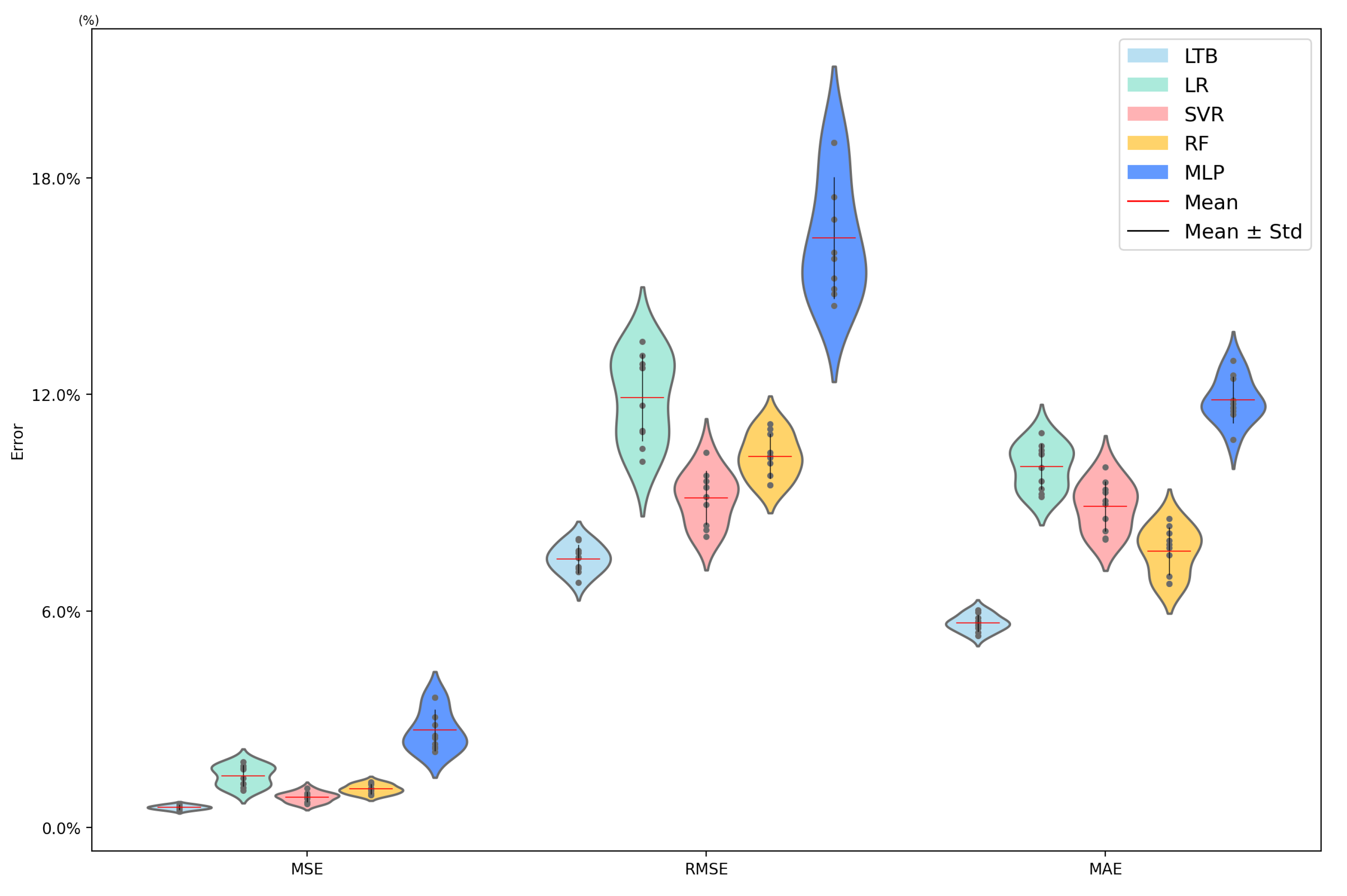
4.2. Load Prediction Results Without Considering Missing Data

To demonstrate the superiority of the LTB algorithm, a comparative analysis was conducted using four mainstream methods: Linear Regression (LR), Support Vector Regression (SVR), Random Forest (RF), and Multi-Layer Perceptron (MLP). LR, SVR, and RF were configured with default parameters, while the number of neurons in the fully connected layer of MLP was set to 64, with 20 iterations. For the LTB algorithm, the base predictor depth was set to 3, the number of base predictors was 20, and the search space for parameter u was [0,1].

To enhance the robustness of the experiment and avoid bias from a single result, all experiments were conducted 10 times with different random train–test splits to evaluate the differences in accuracy and fairness metrics. The dataset was split such that 60% was used for training and 40% for testing and validation. The cutting load prediction results of the five algorithms are presented in

Table 2. Load prediction results without considering missing data.

Method	Load Prediction Result
	MSE	RMSE	MAE
LTB	0.0055	0.0743	0.0566
LR	0.0143	0.1191	0.1000
SVR	0.0084	0.0914	0.0890
RF	0.0106	0.1029	0.0766
MLP	0.0269	0.1633	0.1185

. The data in the table represent the average test errors of each algorithm, including mean squared error (MSE), root mean squared error (RMSE), and mean absolute error (MAE).

Compared to the baseline methods, the proposed LTB algorithm consistently achieves superior prediction accuracy on complete data. Specifically, LTB attains a mean squared error (MSE) of 0.0055, outperforming traditional models such as LR (0.0143), SVR (0.0084), RF (0.0106), and MLP (0.0296). This corresponds to a relative improvement of 34.5% over SVR and 79.6% over MLP. These results highlight LTB’s capability to effectively model nonlinear dependencies in multi-sensor tunneling data while maintaining low prediction variance across repeated trials. In terms of RMSE and MAE, the LTB algorithm also demonstrates the best performance, further confirming its overall predictive advantage.

Additionally, the test results of the 10 repeated experiments are shown in Figure 8. As illustrated in the figure, the proposed LTB method is the most stable across all metrics. The MLP and LR algorithms exhibit significant fluctuations. In contrast, the LTB algorithm is more stable, produces smaller test errors, and outperforms the SVR and RF algorithms across all metrics.

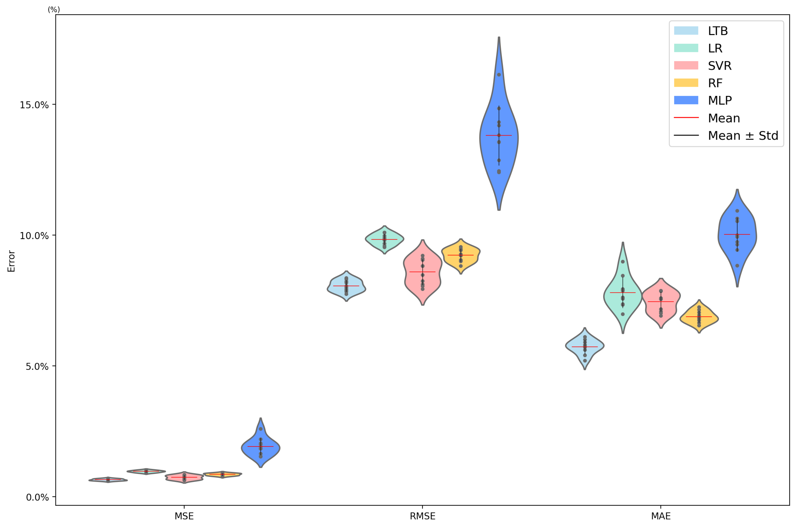
4.3. Load Prediction Results Considering Missing Data

The cutting load prediction results under the missing data condition are shown in

Table 3. Load prediction results without considering missing data.

Method	Load Prediction Result
	MSE	RMSE	MAE
LTB	0.0065	0.0806	0.0572
LR	0.0097	0.0983	0.0781
SVR	0.0074	0.0859	0.0745
RF	0.0085	0.0923	0.0688
MLP	0.0192	0.1382	0.1003

. As indicated in Table 3, despite the presence of partially missing data, the LTB algorithm still demonstrates the best prediction performance. Compared to predictions on the complete dataset, the average MSE, RMSE, and MAE of the LTB algorithm have slightly increased to 0.65%, 8.06%, and 5.72%, respectively. Thanks to data imputation, the performance metrics of the other four comparison methods have improved, and their prediction errors have been further reduced, although they remain higher than those of the LTB algorithm.

The test results of the 10 repeated experiments under the missing data condition are shown in Figure 9. As illustrated in the figure, the proposed LTB method is the most stable across all metrics and outperforms the LR, SVR, RF, and MLP algorithms across all metrics.

Overall, under conditions with 3% missing data, the LTB algorithm continues to deliver the best performance among all compared methods. As shown in Table 3, LTB achieves a mean squared error (MSE) of 0.0065, whereas LR, MLP, RF, and SVR exhibit significantly higher errors of 0.097, 0.074, 0.0085, and 0.0192, respectively. This corresponds to an error reduction of approximately 66.1% compared to MLP and 12.2% compared to SVR. Furthermore, the standard deviation of LTB’s performance across multiple trials remains low, indicating high robustness under partial sensor failures. These results confirm LTB’s ability to preserve accuracy without relying on imputation, a critical advantage in underground environments where sensor dropout is both frequent and unavoidable.

5. Conclusions

Accurate underground cutting load prediction helps to improve the prediction accuracy and reliability of unmanned tunneling systems. The existing underground multi-sensor load prediction methods lack consideration for cutting reliability and safety and do not address the issue of missing underground data, making it difficult to provide reliable support for unmanned mining of deep coal seams. This paper proposes a reliable underground coal–rock cutting load prediction method that considers safety constraints and missing data. It uses a trustworthy decision tree capable of handling missing data as the base predictor and adds cutting safety constraints in the algorithm design to improve prediction reliability.

Extensive comparative experiments were conducted using real-world underground cutting data. On the complete dataset, the proposed LTB model achieved an MSE of 0.0055, outperforming baseline methods such as MLP (0.0296) and SVR (0.0084) with improvements of over 79.6% and 34.5%, respectively. Even under 3% missing data conditions, LTB maintained high accuracy (MSE: 0.0065) and low variance, demonstrating superior robustness without requiring explicit imputation.

By integrating trustworthy machine learning theory with domain-specific safety modeling, this study offers a more reliable framework for load prediction under complex underground conditions. The ability to handle partial observations makes it highly suitable for deployment in sensor-degraded environments, thereby providing a dependable basis for downstream intelligent decision-making.

Future research should focus on extending the proposed framework in several key directions. First, the incorporation of richer multimodal sensing data—such as vibration signatures, acoustic emissions, and thermal imagery—may further improve predictive robustness and situational awareness in complex mining environments. Second, the integration of advanced machine learning paradigms, including attention-based architectures, graph neural networks, and causal inference frameworks, holds promise for enhancing both the expressiveness and interpretability of trust modeling. Finally, large-scale deployment and longitudinal validation in operational mining systems will be critical to assess the framework’s adaptability, stability, and real-time decision-making efficacy under dynamic field conditions.

References

1. Guo, D.; Song, Z.; Liu, N.; Xu, T.; Wang, X.; Zhang, Y.; Su, W.; Cheng, Y. Performance study of hard rock cantilever roadheader based on PCA and DBN. Rock Mech. Rock Eng. 2024, 57, 2605–2623. [Google Scholar] [CrossRef]
2. Cheng, J.; Jiang, H.; Wang, D.; Zheng, W.; Shen, Y.; Wu, M. Analysis of position measurement accuracy of boom-type roadheader based on binocular vision. IEEE Trans. Instrum. Meas. 2024, 73, 5016712. [Google Scholar] [CrossRef]
3. Zhang, J.; Wan, C.; Wang, J.; Chen, C.; Wang, T.; Zhang, R.; Guo, H. Research on the “shape-performance-control” integrated digital twin system for boom-type roadheaders. Sci. Rep. 2024, 14, 5780. [Google Scholar] [CrossRef] [PubMed]
4. Wang, G.; Zhang, L.; Li, S.; Li, S.; Feng, Y.; Meng, L.; Nan, B.; Du, M.; Fu, Z.; Li, R. Progress in the theory and technology development of unmanned intelligent coal mining systems. J. China Coal Soc. 2023, 48, 34–53. [Google Scholar]
5. Ge, S.; Hu, E.; Li, Y. New advances and new directions in coal mine robot technology. J. China Coal Soc. 2023, 48, 54–73. [Google Scholar]
6. Zhang, J.; Tu, S.; Cao, Y.; Tan, Y.; Xin, H.; Pang, J. Intelligent separation and filling technology of coal gangue in underground coal mines and its engineering application. J. China Univ. Min. Technol. 2021, 50, 14. [Google Scholar]
7. Ding, Z. Current status and development trend of coal roadway excavation equipment in China. Ind. Mine Autom. 2014, 40, 5. [Google Scholar]
8. Xu, X.; Peng, S.; Ma, Z.; Zhu, P.; Wang, Y. Principle and key technologies of dynamic detection of coal-rock interface in mines based on air-coupled radar. J. China Coal Soc. 2022, 47, 47. [Google Scholar]
9. Miao, S.; Shao, D.; Liu, Z.; Fan, Q.; Li, S.; Ding, E. Study on coal-rock identification method based on terahertz time-domain spectroscopy technology. Spectrosc. Spectr. Anal. 2022, 42, 1806–1812. [Google Scholar]
10. Chen, G.; Fan, Y.; Li, Q. A study of coalbed methane (CBM) reservoir boundary detection based on azimuth electromagnetic waves. J. Pet. Sci. Eng. 2019, 179, 432–443. [Google Scholar] [CrossRef]
11. Zhao, Y.; Liu, C.; Zheng, Z.; Guo, L.; Ma, Z.; Han, Z. Intelligent vehicle positioning method based on multi-sensor information fusion. J. Automot. Eng. 2021, 11, 10. [Google Scholar]
12. Ding, X. Research on encryption control of multi-sensor information for intelligent robots based on blockchain. Comput. Meas. Control 2021, 196, 103245. [Google Scholar]
13. Xu, A. Research on mobile robot positioning based on fuzzy PID Kalman filter multi-sensor information fusion. J. Chongqing Univ. Sci. Technol. (Nat. Sci. Ed.) 2014, 16, 4. [Google Scholar]
14. Li, J.; Zhang, S.; Gong, Z.; Guo, Q. Fire early warning method for conveyorbelt transport tunnels based on multi-sensor information fusion. Coal Mine Mach. 2017, 38, 4. [Google Scholar]
15. Xie, H.; Tan, F.; Sun, Z. Research and implementation of warehouse alarm system based on multi-sensor fusion and GSM. Sens. World 2008, 31, 38–40. [Google Scholar]
16. Deng, Z.; Li, H. Review of automatic navigation technology for mobile robots. Sci. Technol. Inf. 2016, 33, 142–144. [Google Scholar]
17. Wang, H.; Huang, M.; Gao, X.; Lu, S.; Zhang, Q. Coal-rock interface perception and identification based on multi-sensor information fusion considering cutter wear. J. China Coal Soc. 2021, 46, 14. [Google Scholar]
18. Yang, J.; Fu, S.; Jiang, H.; Zhao, X.; Wu, M. Identification of cutting hardness of coal-rock based on fuzzy criteria. J. China Coal Soc. 2015, 40, 6. [Google Scholar]
19. Ebrahimabadi, A.; Azimipour, M.; Bahreini, A. Prediction of roadheader performance using artificial neural network approaches (MLP and KOSFM). J. Rock Mech. Geotech. Eng. 2015, 7, 573–583. [Google Scholar] [CrossRef]
20. Wang, P.; Mu-Qin, T.; Lin, Y.; Hua, Y.; Na, Z.; Hong, L. Dynamic load identification method of rock roadheader using multi-neural network and evidence theory. Coal Technol. 2018, 1238–1243. [Google Scholar] [CrossRef]
21. Wang, P.; Yang, Y.; Wang, D.; Ji, X.; Shen, Y.; Chen, S.; Li, X.; Wu, M. Intelligent cutting control system and method for cantilever-type roadheader in coal gangue. J. China Coal Soc. 2021, 46, 11. [Google Scholar]
22. Wang, P.; Shen, Y.; Li, R.; Zong, K.; Fu, S.; Wu, M. Multisensor informationbased adaptive control method for cutting head speed of roadheader. Proc. Inst. Mech. Eng. C 2021, 235, 1941–1955. [Google Scholar] [CrossRef]
23. Newman, D.A. Missing data: Five practical guidelines. Organ. Res. Methods 2014, 17, 372–411. [Google Scholar] [CrossRef]
24. Twala, B.; Jones, M.; Hand, D. Good methods for coping with missing data in decision trees. Pattern Recognit. Lett. 2008, 29, 950–956. [Google Scholar] [CrossRef]
25. Jeong, H.; Wang, H.; Calmon, F. Fairness without imputation: A decision tree approach for fair prediction with missing values. In Proceedings of the IEEE International Conference on Big Data, Orlando, FL, USA, 15–18 December 2021. [Google Scholar]
26. Wang, P.; Shen, Y.; Ji, X.; Zong, K.; Zheng, W.; Wang, D.; Wu, M. Multiparameter control strategy and method for cutting arm of roadheader. Shock Vib. 2021, 2021, 9918988. [Google Scholar] [CrossRef]
27. Sobota, P.; Dolipski, M.; Cheluszka, P. Investigating the simulated control of the rotational speed of roadheader cutting heads in relation to the reduction of energy consumption during the cutting process. J. Min. Sci. 2015, 51, 298–308. [Google Scholar]
28. Little, R.J.A.; Rubin, D.B. Statistical Analysis with Missing Data. Technometrics 2002, 45, 364–365. [Google Scholar]
29. Schafer, J.L.; Graham, J.W. Missing data: Our view of the state of the art. Psychol. Methods 2002, 7, 147–177. [Google Scholar] [CrossRef]
30. van Buuren, S.; Groothuis-Oudshoorn, K. MICE: Multivariate Imputation by Chained Equations in R. J. Stat. Softw. 2011, 45, 1–67. [Google Scholar] [CrossRef]
31. Royston, P. Multiple imputation of missing values: Update. Stata J. 2005, 5, 227–241. [Google Scholar] [CrossRef]
32. Tang, F.; Ishwaran, H. Random forest missing data algorithms. Stat. Anal. Data Min. 2017, 10, 363–377. [Google Scholar] [CrossRef] [PubMed]
33. Zhang, Z. Missing data imputation: Focusing on single imputation. Ann. Transl. Med. 2016, 4, 9. [Google Scholar] [PubMed]
34. Bertsimas, D.; Pawlowski, C.; Zhuo, Y.D. From predictive methods to missing data imputation: An optimization approach. J. Mach. Learn. Res. 2018, 18, 1–39. [Google Scholar]
35. Wulff, J.N.; Ejlskov, L. Multiple imputation by chained equations in praxis: Guidelines and review. Electron. J. Bus. Res. Methods 2017, 15, 2017–2058. [Google Scholar]
Figure 1. Field site of the tunneling face. (a) Cantilever roadheader robot. (b) Tunneling and cutting section.
Information 16 00548 g001
Figure 2. Laboratory equipment. (a) Pressure transmitter. (b) Vibration sensor. (c) Data recorder.
Information 16 00548 g002
Figure 3. Cutting load variation trends under different multi-sensor information.
Information 16 00548 g003
Figure 4. Workflow of the proposed load-trustworthy-boosting (LTB) framework.
Information 16 00548 g004
Figure 5. Schematic diagram of the proposed Trust MIP Tree (shown here with depth 2) illustrating how missing sensor values are handled. Each branch node splits on a chosen feature with a threshold (q) when the data is available and uses a binary flag (c) to direct samples when the feature value is missing. Each leaf node outputs a predicted load value (u).
Information 16 00548 g005
Figure 6. Illustration of the load prediction process using a Trust MIP Tree when some sensor data are missing. In this example, a data sample with four sensor features (cutting motor current, lifting cylinder pressure, rotary cylinder pressure, and cutting arm vibration acceleration) is passed through a depth-3 Trust MIP Tree. Branch node 1 splits on feature 2 with threshold q (18.15), sending the sample to the right; branch node 2 splits on feature 1 with threshold q (100.21), sending the sample to the left; branch node 3 encounters a missing value for feature 4, represented by the symbol * in the figure, so it uses the indicator c to direct the sample to the right. A one-hot vector Z indicates which leaf node the sample reaches (leaf 4 in this case), and the corresponding predicted load u (0.91) at that leaf is output as the load prediction.
Information 16 00548 g006
Figure 7. Overall flowchart of the proposed LTB algorithm. The process begins with initializing sample weights. The Trust MIP Tree base predictor is trained and evaluated, and then the error e r is computed and augmented with the safety–trust term to form e m . Safety constraints are incorporated by adjusting e m using the factor μ in the loss function. Next, the weight coefficient α k for the base learner is updated according to the error rates, and sample weights are re-weighted (increasing for mispredicted or unsafe samples). This iterative procedure continues for K rounds, and finally the ensemble model outputs a prediction as the weighted vote of all base predictors.
Information 16 00548 g007
Figure 8. Comparison of load prediction performance on the complete dataset (no missing data) for different algorithms. The results are evaluated in terms of MSE, RMSE, and MAE and are averaged over 10 independent train–test splits. The LTB algorithm achieves the lowest errors and exhibits the least variability across trials, indicating better stability and accuracy compared to the baseline methods (LR, SVR, RF, and MLP).
Information 16 00548 g008
Figure 9. Comparison of load prediction performance under a missing-data scenario (approximately 3% of values missing) for different algorithms. Baseline methods (LR, SVR, RF, and MLP) use k-NN imputation to fill in missing sensor values, whereas LTB handles missing data intrinsically. The error metrics (MSE, RMSE, and MAE) are averaged over 10 trials. The LTB algorithm achieves the highest accuracy and stability across all metrics, outperforming the baseline models even when those models are aided by imputation.
Information 16 00548 g009