HASSDE-NAS: Heuristic–Adaptive Spectral–Spatial Neural Architecture Search with Dynamic Cell Evolution for Hyperspectral Water Body Identification


Abstract
1. Introduction
- Spectral-index approaches leverage band ratios to isolate water pixels but falter under complex spectral interference. Standard spectral indices include the Normalized Difference Water Index (NDWI) [4,5,6], Modified NDWI (MNDWI) [7], enhanced water index [8], automated water index [9,10], and water index 2015 [11]. These methods are usually applied to multispectral data.
- Spatial-feature-based methods enhance identification through structural analysis, including morphological denoising [12], Gabor/wavelet texture descriptors [13], and connectivity modeling via region-growing [14,15] or graph theory [16]. However, their performance degrades significantly in low-contrast or complex-texture scenarios owing to dependencies on image resolution and illumination conditions.
- Machine learning-based methods, such as decision trees [17], random forests [18,19], and SVM [20], rely on manual feature engineering for water body identification; however, they fall short in modeling nonlinear relationships and fail to offer generalizability under complex spectral–spatial coupling conditions.
- Deep learning-based approaches, such as DenseNet [21], U-Net [22], and Transformer [23], enhance classification accuracy through automated feature extraction but demonstrate three key challenges: (1) strong dependance on the experience of experts, (2) the optimal integration of spectral and spatial characteristics, and (3) limited detection capability for small-scale aquatic features such as narrow rivers, particularly where boundary ambiguity arises from mixed water–vegetation edges, and lower accuracy for fragmented water bodies [24].
- This study introduces a cell search algorithm that dynamically evaluates and selects optimal spectral–spatial operations during neural architecture search. This approach continuously assesses architectural stability, feature diversity, and gradient sensitivity across network layers, enabling the adaptive prioritization of task-relevant units while avoiding local optima. The integrated optimization strategy combines adaptive learning rate scheduling with gradient clipping to enhance search efficiency and model robustness for complex water body identification tasks.
- We design a unified differentiable cell structure featuring dynamic path weighting and residual cross-layer connections. This architecture dynamically calibrates operational contributions through learnable gating mechanisms and preserves critical shallow features via channel-aligned skip connections. The specialized operator sets enable task-specific spectral enhancement, boundary refinement, and cross-modal fusion while maintaining computational efficiency.
- Comprehensive evaluation on Gaofen-5 hyperspectral datasets demonstrates unprecedented accuracy in water body identification, achieving 92.61% and 96.00% overall accuracy for the Guangdong and Henan regions, respectively. The framework shows exceptional capability in challenging scenarios, including narrow rivers and low-contrast water bodies under complex environmental interference.
2. Related Work
3. Proposed Method
3.1. Overall Workflow
3.2. Inner Search Architecture
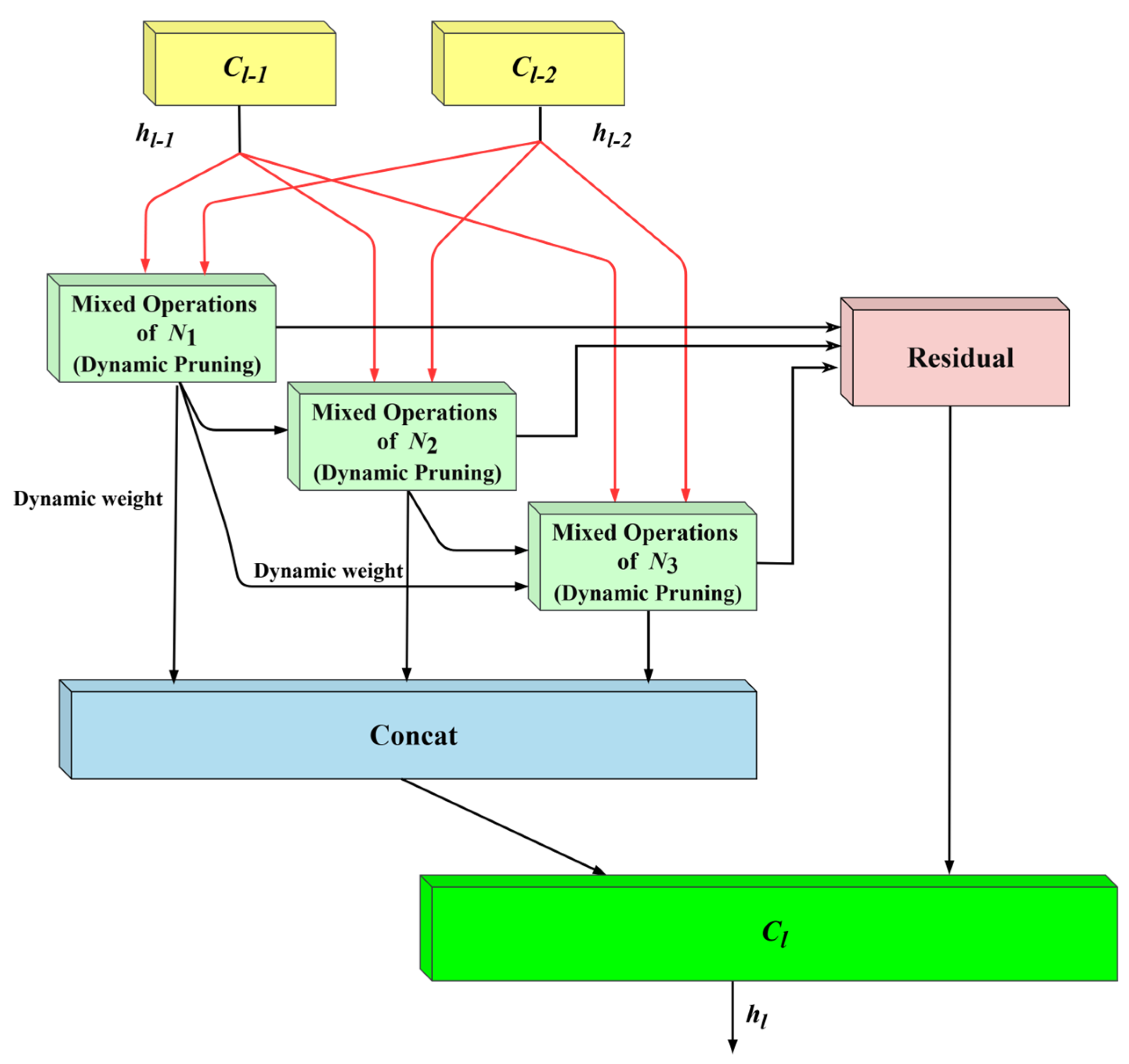
3.2.1. Structure of DRG-Cell
- 1.
- Dynamic Path Weighting Mechanism
- 2.
- Residual Cross-Layer Fusion
- 3.
- Adaptive Pruning Strategy
3.2.2. Set of Candidate Operations
3.3. External Search Network
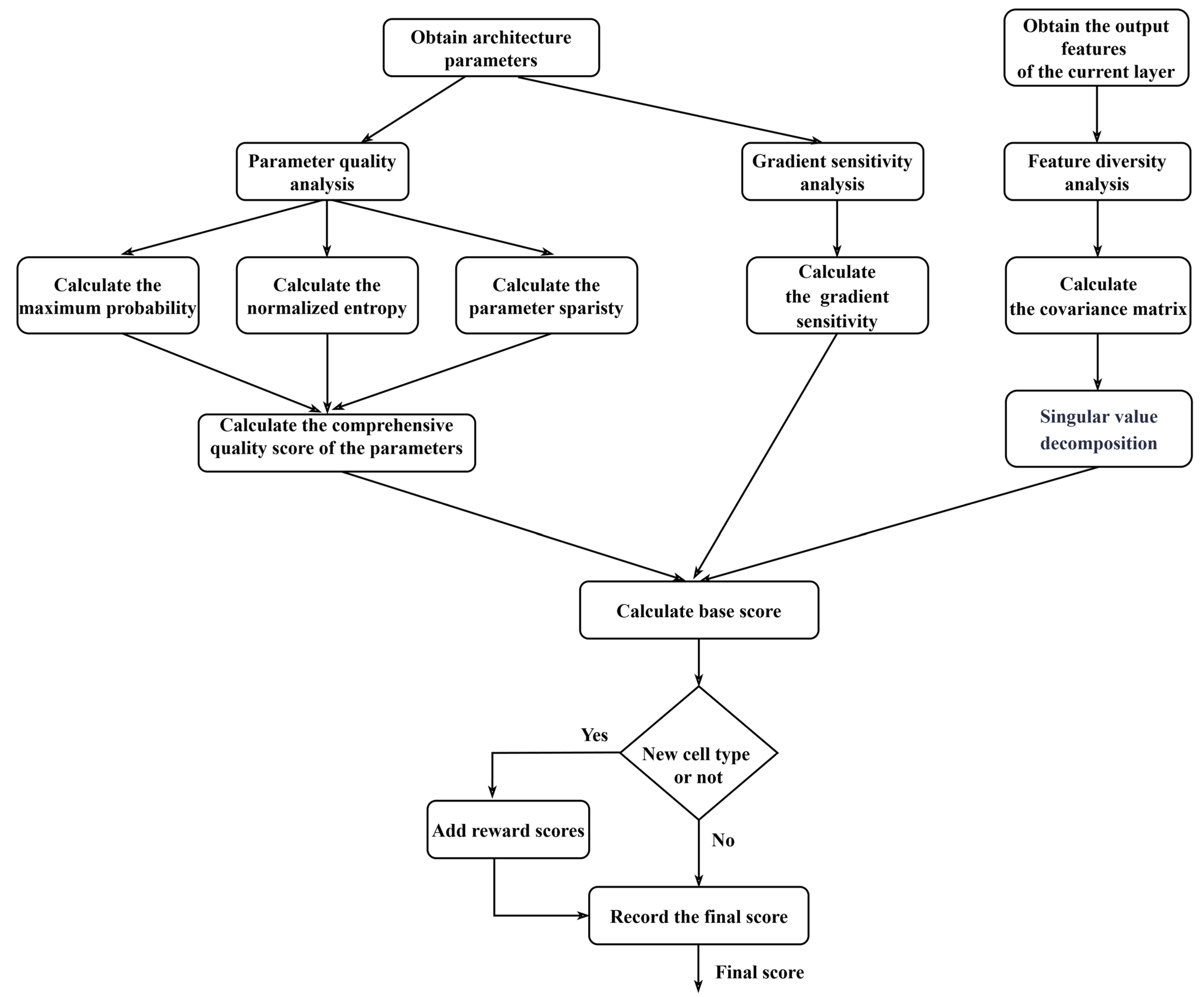
3.4. Multidimensional Dynamic Fusion-Based Heuristic Cell Search Algorithm
- Architecture Stability Analysis.
- 2.
- Feature Diversity Analysis.
- 3.
- Gradient sensitivity analysis.
| Algorithm 1: Heuristic cell search procedure. |
| Input: l: Layer index, X: Features, α/β/δ: Arch params Output: Cell type (DBS, GEA, BFA) 1: // Architecture stability (Equations (8)–(11)) 2: Q_α = [max_prob(α_l) + entropy(α_l) + sparsity(α_l)]/3 3: // Repeat for β, δ 4: // Feature diversity (Equations (12)–(14)) 5: Cov_reg = cov(X_flat) // Regularized covariance 6: D_cell = mean(SVD(Cov_reg)) // Singular values mean 7: // Gradient sensitivity (Equation (15)) 8: S_cell = ∥∇(∑θ)∥2 // Virtual loss gradient 9: // Dynamic fusion (Equation (16)) 10: γ = softmax(arch_gammas [l]) 11: for cell ∈ {DBS, GEA, BFA}: 12: base_score = a·γ_cell + b·Q_cell + c·D_cell + d·S_cell 13: final_score = base_score + (β_div if cell not recent) 14: end for 15: selected_cell = argmax(final_score) 16: return selected_cell // Key aspects: - Q: Param concentration metrics (Equations (8)–(11)) - D: Feature discriminability (Equations (12)–(14)) - S: Optimization stability (Equation (15)) - Diversity bonus prevents local optima - O(N) complexity per layer |
3.5. Loss Function
4. Experiments
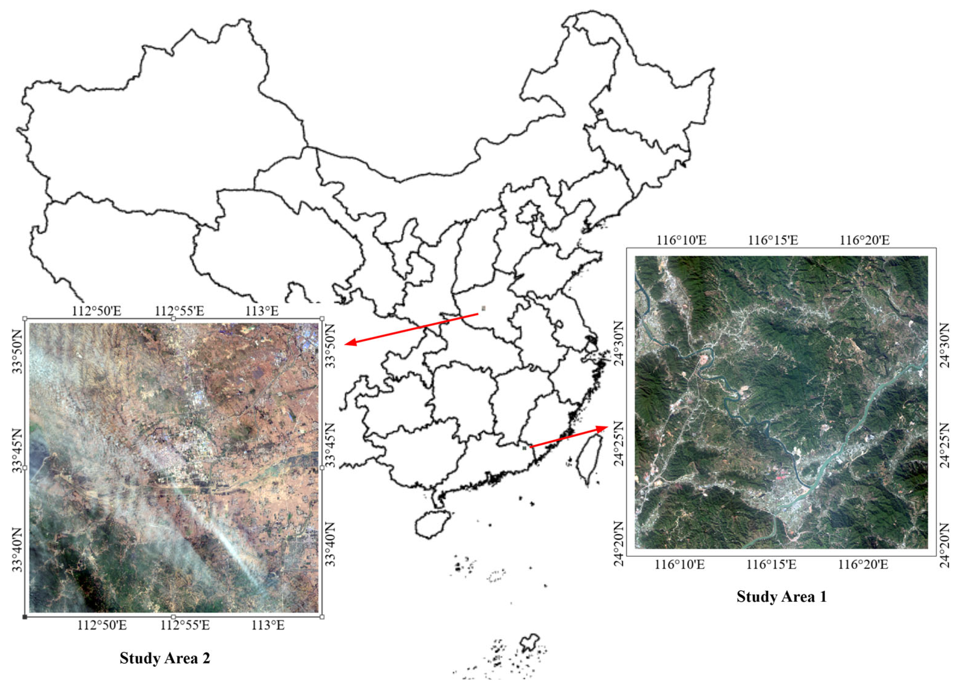
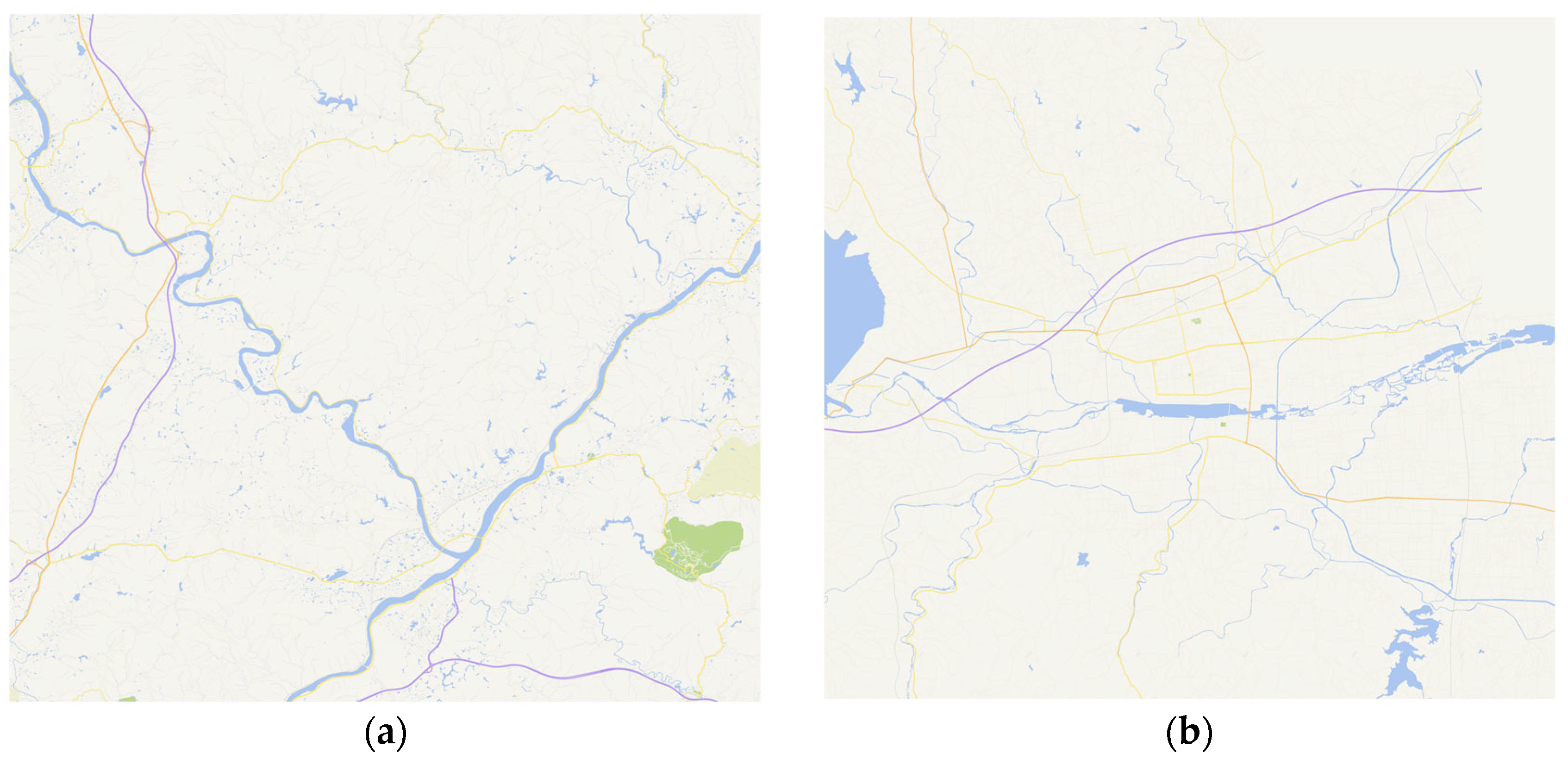
4.1. Study Areas
4.2. Dataset and Preprocessing
4.3. Ground Truth Generation
4.4. Experimental Details
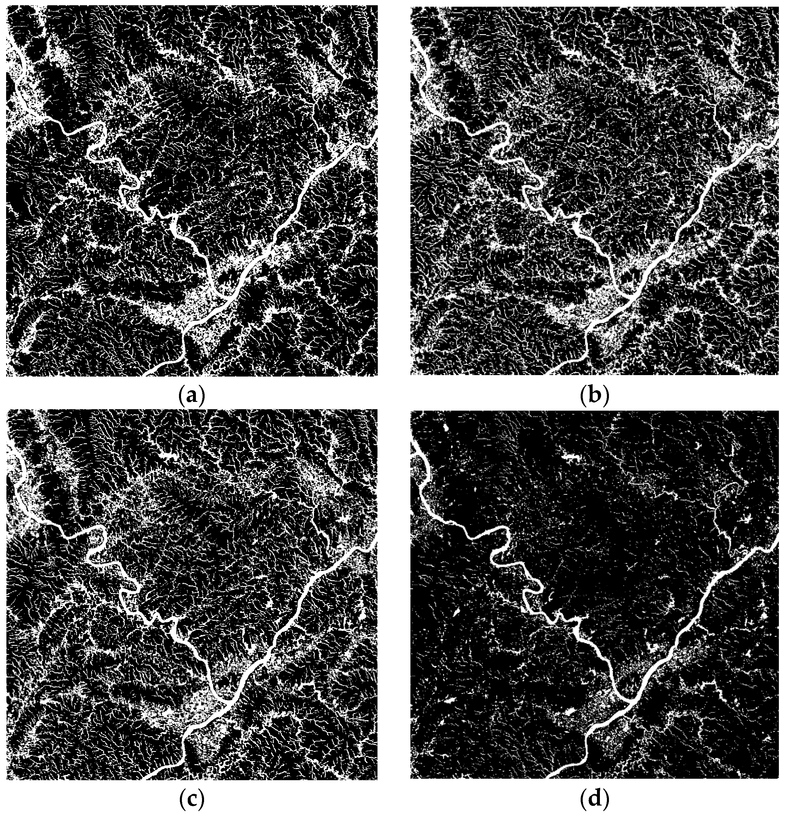
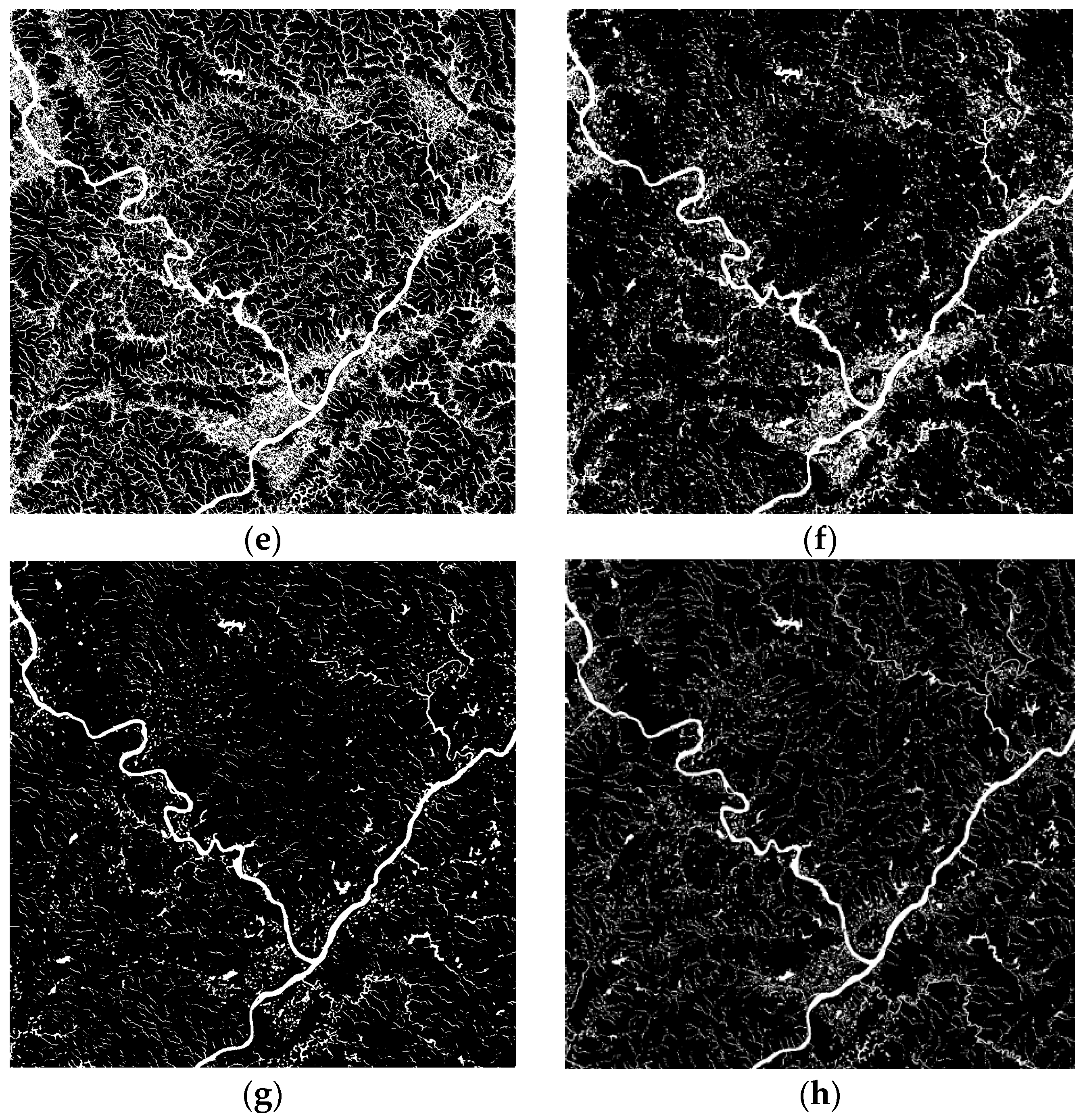
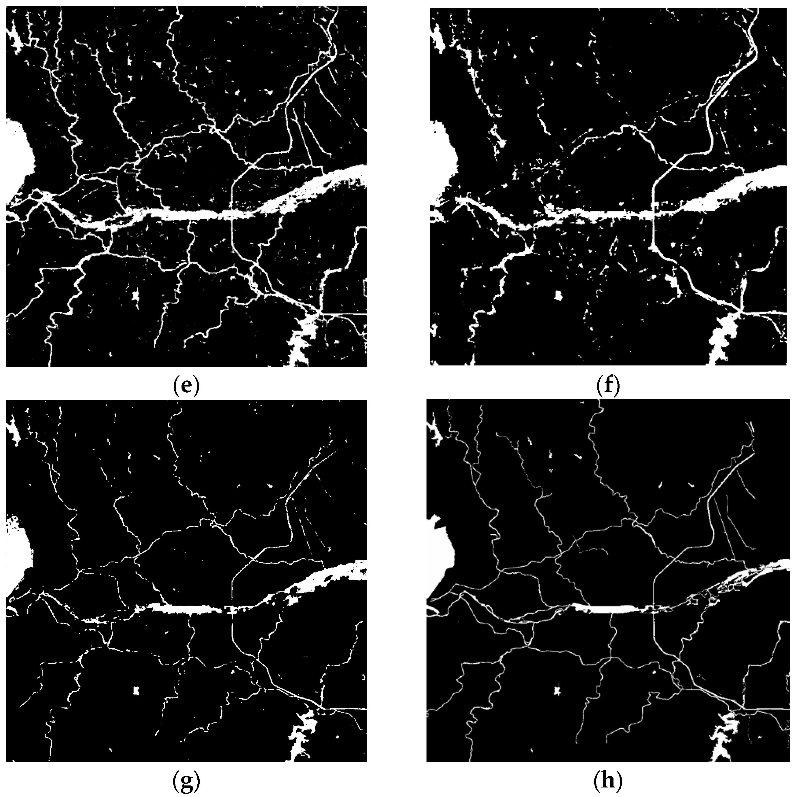
4.5. Comparative Analysis with Other Methods
- SSFTT [52]: This model achieves efficient computation and outstanding classification performance by combining a convolutional neural network with a Transformer architecture and using a Gaussian weighted feature marker to enhance the separability of spectral–spatial features.
- GAHT [53]: This model captures multilevel semantic information through a hierarchical structure and integrates features from different regions using a group perception mechanism. It effectively alleviates excessive feature discretization in traditional Transformer structures and significantly improves classification performance.
- CNCMN [54]: This model expands the feature extraction range by combining pixel-level Euclidean neighbors and superpixel-level non-Euclidean neighbors, enabling it to capture local details and utilize global context information. It adaptively aggregates and fuses the features of the two types of neighbors by fusing image and graph convolution and dynamically screens out information through an attention mechanism, thereby avoiding irrelevant interference and enhancing feature discriminability.
- Hyt-NAS [55]: Hyt-NAS is an HSI classification method that combines NAS with a Transformer. A hybrid search space is designed to handle the low spatial resolution and high spectral resolution of HSIs using the spatial dominant unit and the spectrally dominant unit, respectively.
- HKNAS [56]: HKNAS is an HSI classification method based on a hypernuclear NAS method. By directly generating structural parameters from network weights, the traditional complex double optimization problem is transformed into a single optimization problem, reducing search and model complexity.
- TUH-NAS [57]: TUH-NAS is an HSI classification method based on a three-unit NAS method. A spectral processing unit (SPEU), a spatial processing unit (SPAU), and a feature fusion unit (FFU) are designed to work together, which enhances the deep fusion of spectral and spatial information and improves the classification accuracy.
4.6. Cross-Region Generalization Validation
4.7. Ablation Study
4.8. Analysis of Model Architecture
5. Conclusions
Author Contributions
Funding
Institutional Review Board Statement
Informed Consent Statement
Data Availability Statement
Conflicts of Interest
Abbreviations
| HASSDE-NAS | Heuristic–Adaptive Spectral–Spatial Neural Architecture Search with Dynamic Cell Evaluation |
| NAS | Neural architecture search |
| HSI | Hyperspectral image |
| DARTS | Differentiable architecture search |
| CellDBS | Dynamic band selection cell |
| CellGEA | Geometric edge attention cell |
| CellBFA | Bidirectional fusion alignment cell |
| DRG-Cell | Dynamic residual gated cell |
| MNDWI | Modified Normalized Difference Water Index |
| MF | Matched Filter |
Appendix A. Operation Specification
Appendix A.1. Functional Descriptions
- 1.
- CellDBS: Spectral–Sensitive Unit
- (1)
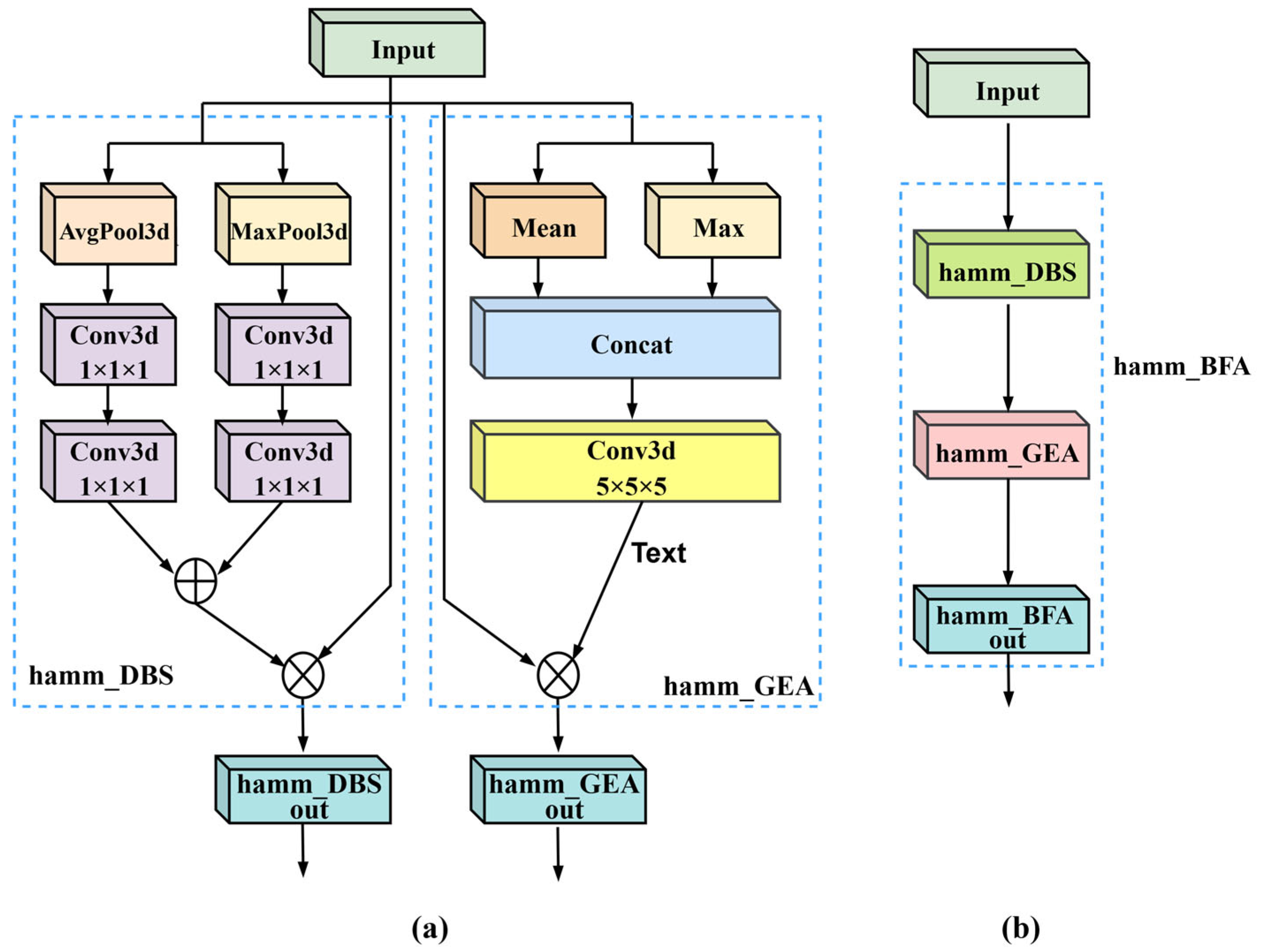
- hamm_DBS: Spectral-dimension attention mechanism.
- (2)
- esep_s3/s5: LeakyReLU-activated 3 × 1 × 1/5 × 1 × 1 separable convolution with BatchNorm.
- (3)
- dilated_3-1/5-1: Dilated convolutions (rate = 2) with kernel sizes 3 × 1 × 1/5 × 1 × 1.
- (4)
- water_enh: Learnable band attention module using soft attention weights followed by 3D convolution for water-specific spectral enhancement.
- (5)
- spec_diff: Adjacent-band differential feature extractor (1D convolution, kernel = 2) with concatenated original features for dimensional recovery.
- (6)
- res_block: Channel attention-enhanced residual module using depthwise separable convolution.
- 2.
- CellGEA: Spatial–Geometric Unit
- (1)
- hamm_GEA: Spatial-dimension attention mechanism.
- (2)
- axial_sep3/5: Axially separable 3 × 3/5 × 5 convolutions processed sequentially along single directions.
- (3)
- dilated_1-3/1-5: Dilated convolutions (rate = 2) with kernel sizes 1 × 3 × 3/1 × 5 × 5.
- (4)
- spa_sep3/5: Spatially orthogonal decomposed 3 × 3/5 × 5 convolutions via horizontal–vertical sequential processing.
- (5)
- res_block: Channel attention-enhanced residual module.
- 3.
- CellBFA: Cross-Modal Fusion Unit
- (1)
- hamm_BFA: Joint spectral–spatial attention mechanism.
- (2)
- dilated_3-3/5-5: Three-dimensional dilated convolutions (kernels = 3 × 3 × 3/5 × 5 × 5).
- (3)
- cross_conv3/5: Two-stage spectral–spatial processing (3 × 1 × 1 → 1 × 3 × 3) to enforce coupled feature learning.
- (4)
- multi_sep3/5: Multi-scale separable 3D convolutions with LeakyReLU activation.
- (5)
- res_block: Channel attention-enhanced residual module.
Appendix A.2. Key Design Distinctions
- (1)
- Spatial decomposition: spa_sep simulates standard convolution through serial horizontal–vertical processing for complex boundaries, whereas axial_sep independently reinforces directional responses for linear water body continuity.
- (2)
- Cross-modal fusion: cross_conv explicitly decouples spectral–spatial learning phases to address mixed pixel issues.
- (3)
- Spectral enhancement: water_enh employs learnable soft attention weights followed by 3D convolution, whereas spec_diff highlights inter-band variations through differential filtering.
References
- Stuart, M.B.; Davies, M.; Hobbs, M.J.; Pering, T.D.; McGonigle, A.J.S.; Willmott, J.R. High-Resolution Hyperspectral Imaging Using Low-Cost Components: Application within Environmental Monitoring Scenarios. Sensors 2022, 22, 4652. [Google Scholar] [CrossRef] [PubMed]
- Yang, S.; Wang, L.; Yuan, Y.; Fan, L.; Wu, Y.; Sun, W.; Yang, G. Recognition of small water bodies under complex terrain based on SAR and optical image fusion algorithm. Sci. Total Environ. 2024, 946, 174329. [Google Scholar] [CrossRef] [PubMed]
- Liu, Y.-N.; Sun, D.-X.; Hu, X.-N.; Ye, X.; Li, Y.-D.; Liu, S.-F.; Cao, K.-Q.; Chai, M.-Y.; Zhou, W.-Y.-N.; Zhang, J.; et al. The Advanced Hyperspectral Imager Aboard China’s GaoFen-5 satellite. IEEE Geosci. Remote Sens. Mag. 2019, 7, 23–32. [Google Scholar] [CrossRef]
- McFeeters, S.K. The use of the Normalized Difference Water Index (NDWI) in the delineation of open water features. Int. J. Remote Sens. 1996, 17, 1425–1432. [Google Scholar] [CrossRef]
- Xu, H. Modification of normalised difference water index (NDWI) to enhance open water features in remotely sensed imagery. Int. J. Remote Sens. 2006, 27, 3025–3033. [Google Scholar] [CrossRef]
- Li, W.; Du, Z.; Ling, F.; Zhou, D.; Wang, H.; Gui, Y.; Sun, B.; Zhang, X. A Comparison of Land Surface Water Mapping Using the Normalized Difference Water Index from TM, ETM plus and ALI. Remote Sens. 2013, 5, 5530–5549. [Google Scholar] [CrossRef]
- Du, Y.; Zhang, Y.; Ling, F.; Wang, Q.; Li, W.; Li, X. Water Bodies’ Mapping from Sentinel-2 Imagery with Modified Normalized Difference Water Index at 10-m Spatial Resolution Produced by Sharpening the SWIR Band. Remote Sens. 2016, 8, 354. [Google Scholar] [CrossRef]
- Jiang, W.; Ni, Y.; Pang, Z.; Li, X.; Ju, H.; He, G.; Lv, J.; Yang, K.; Fu, J.; Qin, X. An Effective Water Body Extraction Method with New Water Index for Sentinel-2 Imagery. Water 2021, 13, 1647. [Google Scholar] [CrossRef]
- Fang-fang, Z.; Bing, Z.; Jun-sheng, L.; Qian, S.; Yuanfeng, W.; Yang, S. Comparative Analysis of Automatic Water Identification Method Based on Multispectral Remote Sensing. Procedia Environ. Sci. 2011, 11, 1482–1487. [Google Scholar] [CrossRef]
- Feyisa, G.L.; Meilby, H.; Fensholt, R.; Proud, S.R. Automated Water Extraction Index: A new technique for surface water mapping using Landsat imagery. Remote Sens. Environ. 2014, 140, 23–35. [Google Scholar] [CrossRef]
- Fisher, A.; Flood, N.; Danaher, T. Comparing Landsat water index methods for automated water classification in eastern Australia. Remote Sens. Environ. 2016, 175, 167–182. [Google Scholar] [CrossRef]
- Vignesh, T.; Thyagharajan, K.K. Water bodies identification from multispectral images using Gabor filter, FCM and canny edge detection methods. In Proceedings of the 2017 International Conference on Information Communication and Embedded Systems (ICICES), Chennai, India, 23–24 February 2017; pp. 1–5. [Google Scholar]
- Kang, S.; Lin, H. Wavelet analysis of hydrological and water quality signals in an agricultural watershed. J. Hydrol. 2007, 338, 1–14. [Google Scholar] [CrossRef]
- Jin, S.; Liu, Y.; Fagherazzi, S.; Mi, H.; Qiao, G.; Xu, W.; Sun, C.; Liu, Y.; Zhao, B.; Fichot, C.G. River body extraction from sentinel-2A/B MSI images based on an adaptive multi-scale region growth method. Remote Sens. Environ. 2021, 255, 112297. [Google Scholar] [CrossRef]
- Kadapala, B.K.R.; Hakeem, A.K. Region-Growing-Based Automatic Localized Adaptive Thresholding Algorithm for Water Extraction Using Sentinel-2 MSI Imagery. IEEE Trans. Geosci. Remote Sens. 2023, 61, 4201708. [Google Scholar] [CrossRef]
- Wang, Z.; Li, J.; Lin, Y.; Meng, Y.; Liu, J. GrabRiver: Graph-Theory-Based River Width Extraction From Remote Sensing Imagery. IEEE Geosci. Remote Sens. Lett. 2022, 19, 1500505. [Google Scholar] [CrossRef]
- Crasto, N.; Hopkinson, C.; Forbes, D.L.; Lesack, L.; Marsh, P.; Spooner, I.; van der Sanden, J.J. A LiDAR-based decision-tree classification of open water surfaces in an Arctic delta. Remote Sens. Environ. 2015, 164, 90–102. [Google Scholar] [CrossRef]
- Acharya, T.D.; Lee, D.H.; Yang, I.T.; Lee, J.K. Identification of Water Bodies in a Landsat 8 OLI Image Using a J48 Decision Tree. Sensors 2016, 16, 1075. [Google Scholar] [CrossRef]
- Li, X.; Ding, J.; Ilyas, N. Machine learning method for quick identification of water quality index (WQI) based on Sentinel-2 MSI data: Ebinur Lake case study. Water Supply 2021, 21, 1291–1312. [Google Scholar] [CrossRef]
- Huang, X.; Xie, C.; Fang, X.; Zhang, L. Combining Pixel- and Object-Based Machine Learning for Identification of Water-Body Types From Urban High-Resolution Remote-Sensing Imagery. IEEE J. Sel. Top. Appl. Earth Obs. Remote Sens. 2015, 8, 2097–2110. [Google Scholar] [CrossRef]
- Wang, G.; Wu, M.; Wei, X.; Song, H. Water Identification from High-Resolution Remote Sensing Images Based on Multidimensional Densely Connected Convolutional Neural Networks. Remote Sens. 2020, 12, 795. [Google Scholar] [CrossRef]
- Wang, M.; Li, C.; Yang, X.; Chu, D.; Zhou, Z.; Lau, R.Y.K. QTU-Net: Quaternion Transformer-Based U-Net for Water Body Extraction of RGB Satellite Image. IEEE Trans. Geosci. Remote Sens. 2024, 62, 5634816. [Google Scholar] [CrossRef]
- Kang, J.; Guan, H.; Ma, L.; Wang, L.; Xu, Z.; Li, J. WaterFormer: A coupled transformer and CNN network for waterbody detection in optical remotely-sensed imagery. Isprs J. Photogramm. Remote Sens. 2023, 206, 222–241. [Google Scholar] [CrossRef]
- Tayer, T.C.; Douglas, M.M.; Cordeiro, M.C.R.; Tayer, A.D.N.; Callow, J.N.; Beesley, L.; McFarlane, D. Improving the accuracy of the Water Detect algorithm using Sentinel-2, Planetscope and sharpened imagery: A case study in an intermittent river. Giscience Remote Sens. 2023, 60, 2168676. [Google Scholar] [CrossRef]
- Zoph, B.; Le, Q.V. Neural Architecture Search with Reinforcement Learning. arXiv 2016, arXiv:1611.01578. [Google Scholar] [CrossRef]
- Zeng, J.; Xue, Z.; Zhang, L.; Lan, Q.; Zhang, M. Multistage Relation Network With Dual-Metric for Few-Shot Hyperspectral Image Classification. IEEE Trans. Geosci. Remote Sens. 2023, 61, 5510017. [Google Scholar] [CrossRef]
- Zoph, B.; Vasudevan, V.; Shlens, J.; Le, Q.V. Learning Transferable Architectures for Scalable Image Recognition. arXiv 2017, arXiv:1707.07012. [Google Scholar] [CrossRef]
- Pham, H.; Guan, M.; Zoph, B.; Le, Q.; Dean, J. Efficient Neural Architecture Search via Parameters Sharing. In Proceedings of the 35th International Conference on Machine Learning, Proceedings of Machine Learning Research, Stockholm, Sweden, 10–15 July 2018; pp. 4095–4104. [Google Scholar]
- Liu, H.; Simonyan, K.; Yang, Y. DARTS: Differentiable Architecture Search. arXiv 2018, arXiv:1806.09055. [Google Scholar] [CrossRef]
- Feng, W.; Sui, H.; Huang, W.; Xu, C.; An, K. Water Body Extraction From Very High-Resolution Remote Sensing Imagery Using Deep U-Net and a Superpixel-Based Conditional Random Field Model. IEEE Geosci. Remote Sens. Lett. 2019, 16, 618–622. [Google Scholar] [CrossRef]
- Cao, H.; Tian, Y.; Liu, Y.; Wang, R. Water body extraction from high spatial resolution remote sensing images based on enhanced U-Net and multi-scale information fusion. Sci. Rep. 2024, 14, 16132. [Google Scholar] [CrossRef]
- Wang, Y.; Li, Y.; Chen, W.; Li, Y.; Dang, B. DNAS: Decoupling Neural Architecture Search for High-Resolution Remote Sensing Image Semantic Segmentation. Remote Sens. 2022, 14, 3864. [Google Scholar] [CrossRef]
- Pan, H.; Yan, H.; Ge, H.; Wang, L.; Shi, C. Pyramid Cascaded Convolutional Neural Network with Graph Convolution for Hyperspectral Image Classification. Remote Sens. 2024, 16, 2942. [Google Scholar] [CrossRef]
- Fang, Y.; Sun, L.; Zheng, Y.; Wu, Z. Deformable Convolution-Enhanced Hierarchical Transformer With Spectral-Spatial Cluster Attention for Hyperspectral Image Classification. IEEE Trans. Image Process. 2025, 34, 701–716. [Google Scholar] [CrossRef] [PubMed]
- Li, Z.; Cui, X.; Wang, L.; Zhang, H.; Zhu, X.; Zhang, Y. Spectral and Spatial Global Context Attention for Hyperspectral Image Classification. Remote Sens. 2021, 13, 771. [Google Scholar] [CrossRef]
- Wang, J.; Huang, R.; Guo, S.; Li, L.; Zhu, M.; Yang, S.; Jiao, L. NAS-Guided Lightweight Multiscale Attention Fusion Network for Hyperspectral Image Classification. IEEE Trans. Geosci. Remote Sens. 2021, 59, 8754–8767. [Google Scholar] [CrossRef]
- Feng, J.; Bai, G.; Gao, Z.; Zhang, X.; Tang, X. Automatic Design Recurrent Neural Network for Hyperspectral Image Classification. In Proceedings of the 2021 IEEE International Geoscience and Remote Sensing Symposium IGARSS, Brussels, Belgium, 11–16 July 2021; pp. 2234–2237. [Google Scholar]
- Ge, Z.; Cao, G.; Shi, H.; Zhang, Y.; Li, X.; Fu, P. Compound Multiscale Weak Dense Network with Hybrid Attention for Hyperspectral Image Classification. Remote Sens. 2021, 13, 3305. [Google Scholar] [CrossRef]
- Woo, S.; Park, J.; Lee, J.-Y.; Kweon, I.S. CBAM: Convolutional Block Attention Module. arXiv 2018, arXiv:1807.06521. [Google Scholar] [CrossRef]
- Zhong, G.; Wang, L.-N.; Ling, X.; Dong, J. An overview on data representation learning: From traditional feature learning to recent deep learning. J. Financ. Data Sci. 2016, 2, 265–278. [Google Scholar] [CrossRef]
- Ghafari, S.; Tarnik, M.G.; Yazdi, H.S. Robustness of convolutional neural network models in hyperspectral noisy datasets with loss functions. Comput. Electr. Eng. 2021, 90, 107009. [Google Scholar] [CrossRef]
- Yeung, M.; Sala, E.; Schoenlieb, C.-B.; Rundo, L. Unified Focal loss: Generalising Dice and cross entropy-based losses to handle class imbalanced medical image segmentation. Comput. Med. Imaging Graph. 2022, 95, 102026. [Google Scholar] [CrossRef]
- Cai, J.; Wang, S.; Xu, C.; Guo, W. Unsupervised deep clustering via contractive feature representation and focal loss. Pattern Recognit. 2022, 123, 102026. [Google Scholar] [CrossRef]
- Chi, Y.; Zhang, N.; Jin, L.; Liao, S.; Zhang, H.; Chen, L. Comparative Analysis of GF-5 and Sentinel-2A Fusion Methods for Lithological Classification: The Tuanjie Peak, Xinjiang Case Study. Sensors 2024, 24, 1267. [Google Scholar] [CrossRef] [PubMed]
- Han, Y.; Shi, H.; Li, Z.; Luo, H.; Ding, Y.; Xiong, W.; Hu, Z. Greenhouse gas monitoring instrument on the GF-5 satellite-II: On-orbit spectral calibration. Appl. Opt. 2023, 62, 5839–5849. [Google Scholar] [CrossRef] [PubMed]
- Schneider, W. Land Cover Mapping from Optical Satellite Images Employing Subpixel Segmentation and Radiometric Calibration. In Machine Vision and Advanced Image Processing in Remote Sensing, Proceedings of the Concerted Action MAVIRIC; Springer: Berlin/Heidelberg, Germany, 1999; pp. 229–237. [Google Scholar]
- Alkhazur, M. Evaluation of computational radiometric and spectral sensor calibration techniques. In Proceedings of the SPIE 9896, Optics, Photonics and Digital Technologies for Imaging Applications IV, Brussels, Belgium, 29 April 2016; p. 98960O. [Google Scholar]
- Lin, C.; Wu, C.-C.; Tsogt, K.; Ouyang, Y.-C.; Chang, C.-I. Effects of atmospheric correction and pansharpening on LULC classification accuracy using WorldView-2 imagery. Inf. Process. Agric. 2015, 2, 25–36. [Google Scholar] [CrossRef]
- Qiao, Y.; Tan, Q.; Cui, K. Research on Automatic Generation Technology of Earthquake Emergency Thematic Map Based on MapWorld API. In Proceedings of the 2023 IEEE 13th International Conference on Electronics Information and Emergency Communication (ICEIEC), Beijing, China, 14–16 July 2023; pp. 1–4. [Google Scholar]
- Kaplan, G.; Avdan, U. Object-based water body extraction model using Sentinel-2 satellite imagery. Eur. J. Remote Sens. 2017, 50, 137–143. [Google Scholar] [CrossRef]
- GB/T 35648-2017; Classification and Coding of Geographic Information Points of Interest. General Administration of Quality Supervision, Inspection and Quarantine of the People’s Republic of China, National Standardization Administration: Beijing, China, 2017.
- Sun, L.; Zhao, G.; Zheng, Y.; Wu, Z. SpectralSpatial Feature Tokenization Transformer for Hyperspectral Image Classification. IEEE Trans. Geosci. Remote Sens. 2022, 60, 5522214. [Google Scholar] [CrossRef]
- Mei, S.; Song, C.; Ma, M.; Xu, F. Hyperspectral Image Classification Using Group-Aware Hierarchical Transformer. IEEE Trans. Geosci. Remote Sens. 2022, 60, 5539014. [Google Scholar] [CrossRef]
- Liu, Q.; Xiao, L.; Huang, N.; Tang, J. Composite Neighbor-Aware Convolutional Metric Networks for Hyperspectral Image Classification. IEEE Trans. Neural Netw. Learn. Syst. 2024, 35, 9297–9311. [Google Scholar] [CrossRef]
- Xue, X.; Zhang, H.; Fang, B.; Bai, Z.; Li, Y. Grafting Transformer on Automatically Designed Convolutional Neural Network for Hyperspectral Image Classification. IEEE Trans. Geosci. Remote Sens. 2022, 60, 5531116. [Google Scholar] [CrossRef]
- Wang, D.; Du, B.; Zhang, L.; Tao, D. HKNAS: Classification of Hyperspectral Imagery Based on Hyper Kernel Neural Architecture Search. IEEE Trans. Neural Netw. Learn. Syst. 2024, 35, 13631–13645. [Google Scholar] [CrossRef]
- Chen, F.; Su, B.S.; Jia, Z.P. TUH-NAS: A Triple-Unit NAS Network for Hyperspectral Image Classification. Sensors 2024, 24, 7834. [Google Scholar] [CrossRef]


| No. | CellDBS | CellGEA | CellBFA |
|---|---|---|---|
| 1 | hamm_DBS | hamm_GEA | hamm_BFA |
| 2 | esep_s3 | axial_sep3 | multi_sep3 |
| 3 | esep_s5 | axial_sep5 | multi_sep 5 |
| 4 | dilated_3-1 | dilated_1-3 | dilated_3-3 |
| 5 | dilated_5-1 | dilated_1-5 | dilated_5-5 |
| 6 | water_enh | spat_sep3 | cross_conv3 |
| 7 | spec_diff | spat_sep5 | cross_conv5 |
| 8 | res_block | res_block | res_block |
| Dataset | Training | Validation | Test | Training % |
|---|---|---|---|---|
| Guangdong | 45,000 | 15,000 | 750,000 | 5.6% |
| Henan | 25,500 | 8500 | 776,000 | 3.1% |
| Dataset | SSFTT | GAHT | CNCMN | Hyt-NAS | 3DHKNAS | TUH-NAS | HASSDE-NAS |
|---|---|---|---|---|---|---|---|
| OA (%) | 82.38 | 82.16 | 80.94 | 87.50 | 81.15 | 86.62 | 92.61 |
| Kappa (×100) | 30.76 | 39.38 | 28.67 | 32.10 | 28.76 | 30.20 | 40.90 |
| Water IoU (×100) | 23.10 | 31.20 | 21.57 | 23.26 | 21.62 | 22.14 | 28.85 |
| Background IoU (×100) | 81.40 | 80.60 | 79.89 | 87.01 | 80.11 | 86.09 | 92.38 |
| F1 score (×100) | 37.50 | 47.50 | 35.49 | 37.70 | 62.25 | 36.30 | 44.80 |
| Dataset | SSFTT | GAHT | CNCMN | Hyt-NAS | 3DHKNAS | TUH-NAS | HASSDE-NAS |
|---|---|---|---|---|---|---|---|
| OA (%) | 91.74 | 92.00 | 92.31 | 95.25 | 94.21 | 95.99 | 96.00 |
| Kappa (×100) | 29.32 | 30.34 | 41.79 | 39.40 | 48.98 | 36.50 | 49.40 |
| Water IoU (×100) | 18.80 | 19.50 | 28.80 | 26.42 | 37.27 | 23.89 | 34.56 |
| Background IoU (×100) | 94.30 | 91.80 | 92.06 | 95.17 | 94.11 | 95.94 | 95.92 |
| F1 score (×100) | 31.70 | 32.60 | 44.72 | 41.80 | 75.71 | 38.60 | 51.40 |
| Method | Test Region | OA(%) | Kappa (×100) | Water IoU (×100) | Background IoU (×100) | F1 (×100) | Time(s) |
|---|---|---|---|---|---|---|---|
| MNDWI | Guangdong | 90.28 | 33.21 | 23.70 | 89.97 | 38.32 | 0.0058 |
| MF | Guangdong | 92.48 | 30.03 | 19.17 | 92.35 | 32.17 | 0.4123 |
| HASSDE-NAS (H→G) | Guangdong | 92.66 | 41.4 | 29.17 | 92.43 | 45.2 | 111,253 |
| HASSDE-NAS (Guangdong) | Guangdong | 92.61 | 40.9 | 28.85 | 92.38 | 44.8 | 111,236 |
| MNDWI | Henan | 57.38 | 4.86 | 7.40 | 55.88 | 13.78 | 0.0052 |
| MF | Henan | 95.76 | 43.25 | 29.17 | 95.69 | 45.17 | 0.4206 |
| HASSDE-NAS (G→H) | Henan | 95.89 | 45.6 | 31.24 | 95.82 | 47.6 | 111,264 |
| HASSDE-NAS (Henan) | Henan | 96.00 | 49.4 | 34.56 | 95.92 | 51.4 | 111,232 |
| G1 | G2 | G3 | HASSDE-NAS | |
|---|---|---|---|---|
| OA (%) | 92.38 | 92.56 | 90.26 | 92.61 |
| Kappa (×100) | 37.60 | 36.10 | 40.30 | 40.90 |
| Water IoU (×100) | 25.77 | 24.99 | 28.78 | 28.85 |
| Background IoU (×100) | 93.54 | 92.37 | 93.01 | 92.38 |
| F1 score (×100) | 41.00 | 40.02 | 42.62 | 44.80 |
Disclaimer/Publisher’s Note: The statements, opinions and data contained in all publications are solely those of the individual author(s) and contributor(s) and not of MDPI and/or the editor(s). MDPI and/or the editor(s) disclaim responsibility for any injury to people or property resulting from any ideas, methods, instructions or products referred to in the content. |
© 2025 by the authors. Licensee MDPI, Basel, Switzerland. This article is an open access article distributed under the terms and conditions of the Creative Commons Attribution (CC BY) license (https://creativecommons.org/licenses/by/4.0/).
Share and Cite
Chen, F.; Su, B.; Jia, Z. HASSDE-NAS: Heuristic–Adaptive Spectral–Spatial Neural Architecture Search with Dynamic Cell Evolution for Hyperspectral Water Body Identification. Information 2025, 16, 495. https://doi.org/10.3390/info16060495
Chen F, Su B, Jia Z. HASSDE-NAS: Heuristic–Adaptive Spectral–Spatial Neural Architecture Search with Dynamic Cell Evolution for Hyperspectral Water Body Identification. Information. 2025; 16(6):495. https://doi.org/10.3390/info16060495
Chicago/Turabian StyleChen, Feng, Baishun Su, and Zongpu Jia. 2025. "HASSDE-NAS: Heuristic–Adaptive Spectral–Spatial Neural Architecture Search with Dynamic Cell Evolution for Hyperspectral Water Body Identification" Information 16, no. 6: 495. https://doi.org/10.3390/info16060495
APA StyleChen, F., Su, B., & Jia, Z. (2025). HASSDE-NAS: Heuristic–Adaptive Spectral–Spatial Neural Architecture Search with Dynamic Cell Evolution for Hyperspectral Water Body Identification. Information, 16(6), 495. https://doi.org/10.3390/info16060495