
FIM-JFF: Lightweight and Fine-Grained Visual UAV Localization Algorithms in Complex Urban Electromagnetic Environments


Abstract
1. Introduction
2. Related Works
2.1. Image Matching Techniques
2.2. UAV Localization Techniques
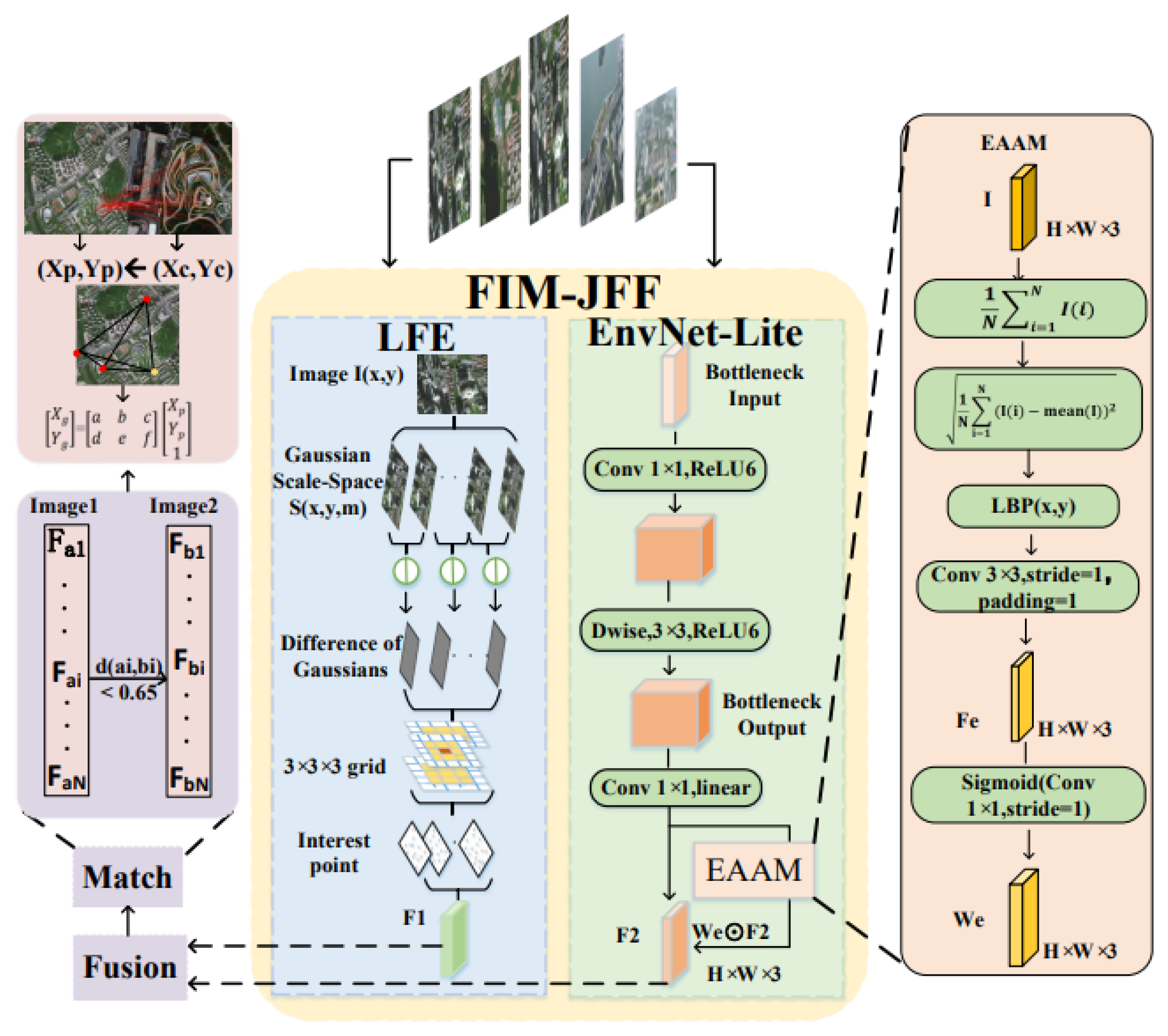
3. Methods
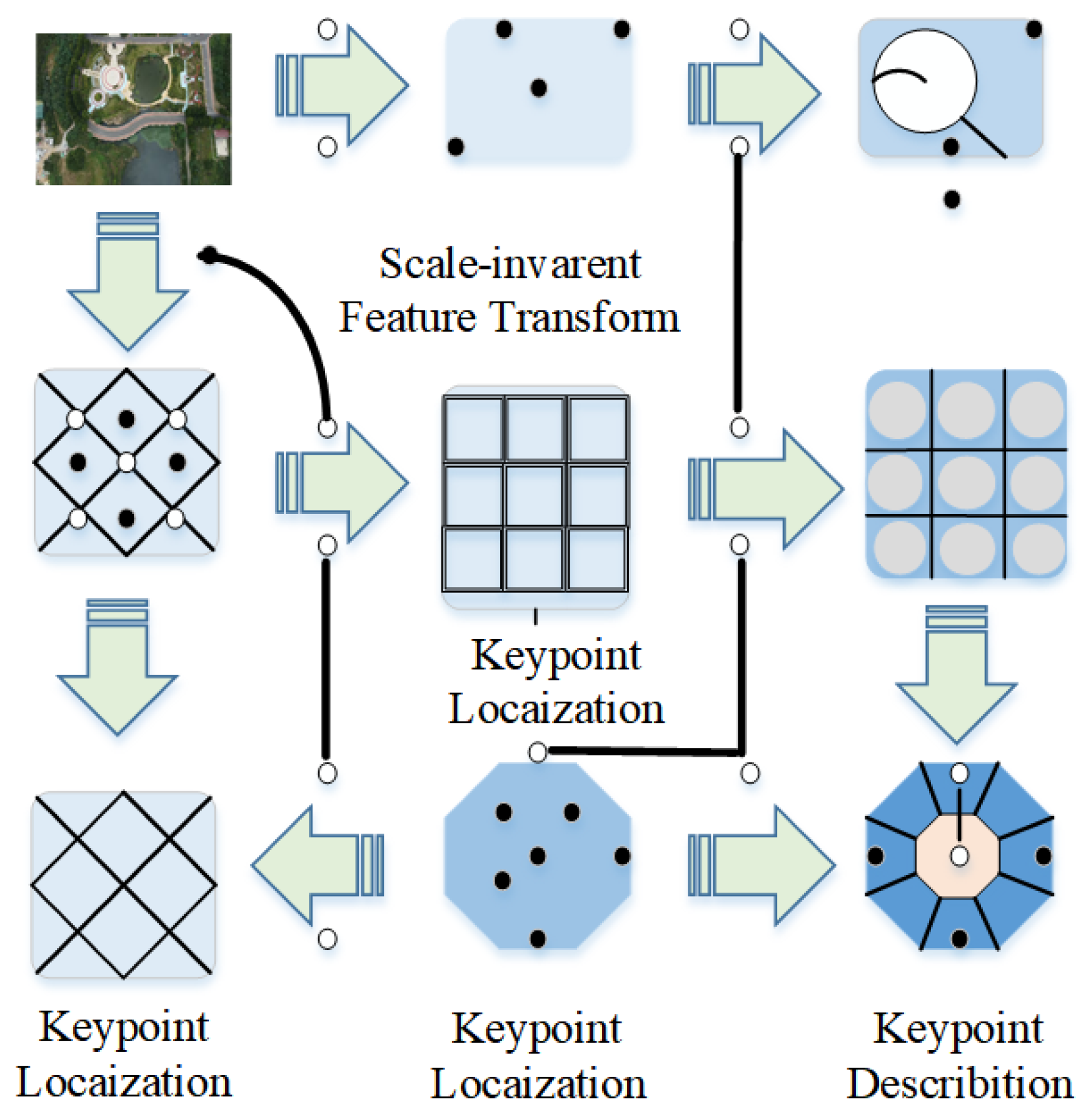
3.1. LFE Module
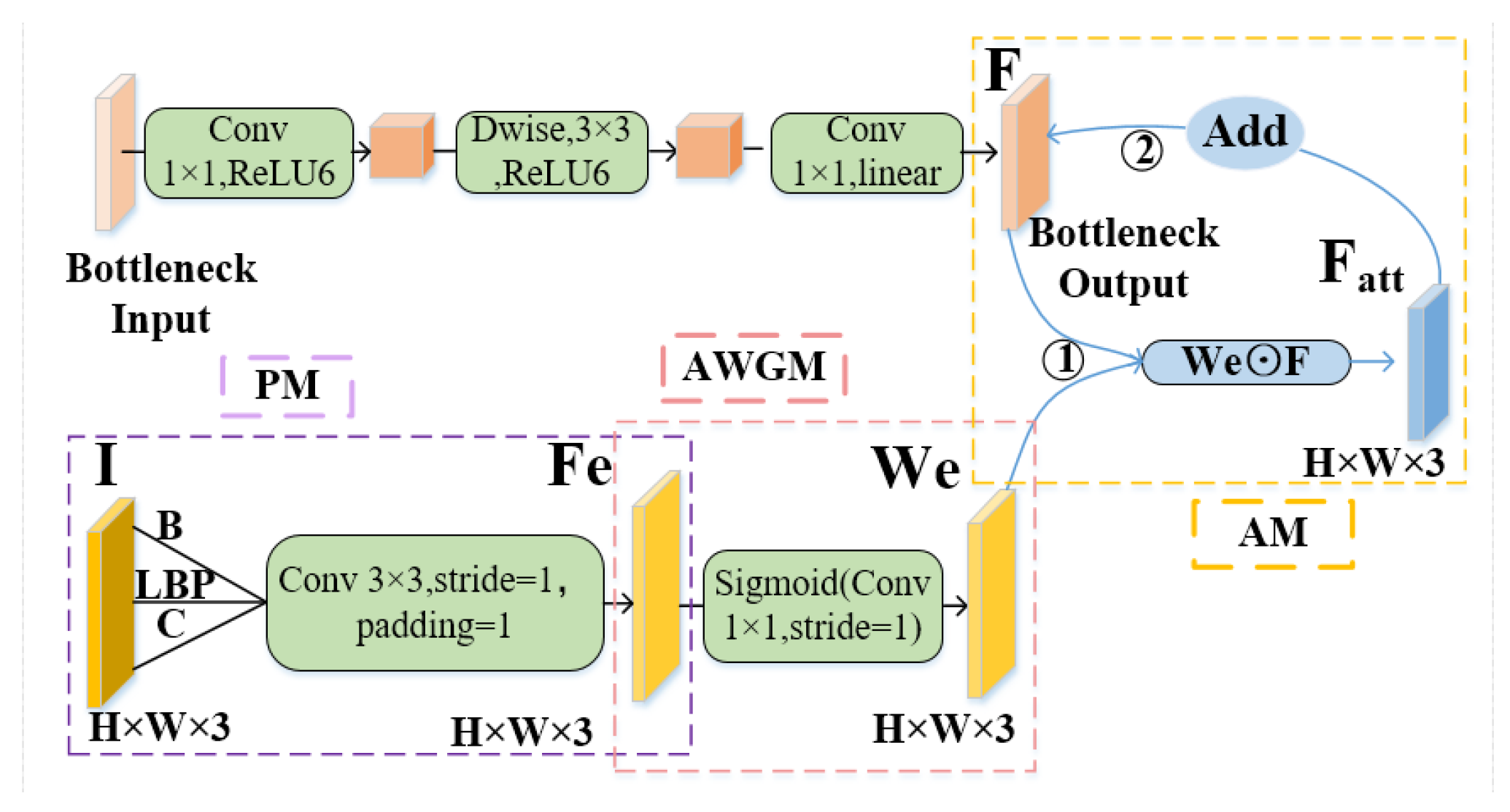
3.2. EnvNet-Lite Module
3.3. Feature Fusion and Matching Module
3.4. Positioning
4. Results
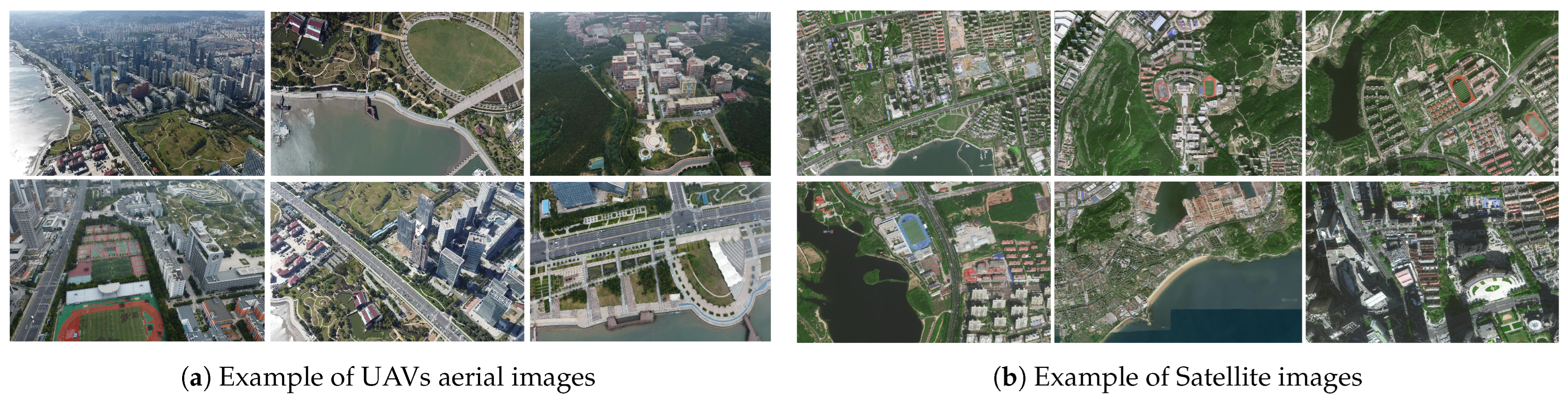
4.1. Experimental Dataset
4.2. Experimental Setup
4.3. FIM-JFF Performance Evaluation
4.3.1. Quantitative Analysis
4.3.2. Qualitative Analysis
4.4. Comparison of Feature Point Extraction Algorithms
4.5. Lightweight Network Performance Comparison
4.6. Ablation Experiments
4.7. Discussion
5. Conclusions
Author Contributions
Funding
Data Availability Statement
Acknowledgments
Conflicts of Interest
References
- Banerjee, B.P.; Raval, S.; Cullen, P. UAV-hyperspectral imaging of spectrally complex environments. Int. J. Remote Sens. 2020, 41, 4136–4159. [Google Scholar] [CrossRef]
- Fan, B.; Li, Y.; Zhang, R.; Fu, Q. Review on the technological development and application of UAV systems. Chin. J. Electron. 2020, 29, 199–207. [Google Scholar] [CrossRef]
- Tian, X.; Shao, J.; Ouyang, D.; Shen, H.T. UAV-satellite view synthesis for cross-view geo-localization. IEEE Trans. Circuits Syst. Video Technol. 2021, 32, 4804–4815. [Google Scholar] [CrossRef]
- Cesetti, A.; Frontoni, E.; Mancini, A.; Ascani, A.; Zingaretti, P.; Longhi, S. A visual global positioning system for unmanned aerial vehicles used in photogrammetric applications. J. Intell. Robot. Syst. 2011, 61, 157–168. [Google Scholar] [CrossRef]
- Ding, G.; Liu, J.; Li, D.; Fu, X.; Zhou, Y.; Zhang, M.; Li, W.; Wang, Y.; Li, C.; Geng, X. A Cross-Stage Focused Small Object Detection Network for Unmanned Aerial Vehicle Assisted Maritime Applications. J. Mar. Sci. Eng. 2025, 13, 82. [Google Scholar] [CrossRef]
- Chen, N.; Fan, J.; Yuan, J.; Zheng, E. OBTPN: A Vision-Based Network for UAV Geo-Localization in Multi-Altitude Environments. Drones 2025, 9, 33. [Google Scholar] [CrossRef]
- Couturier, A.; Akhloufi, M.A. A review on absolute visual localization for UAV. Robot. Auton. Syst. 2021, 135, 103666. [Google Scholar] [CrossRef]
- Arafat, M.Y.; Alam, M.M.; Moh, S. Vision-based navigation techniques for unmanned aerial vehicles: Review and challenges. Drones 2023, 7, 89. [Google Scholar] [CrossRef]
- Aiger, D.; Araujo, A.; Lynen, S. Yes, We CANN: Constrained Approximate Nearest Neighbors for Local Feature-Based Visual Localization. In Proceedings of the IEEE/CVF International Conference on Computer Vision, Paris, France, 1–6 October 2023; pp. 13339–13349. [Google Scholar]
- Zhao, X.; Shi, Z.; Wang, Y.; Niu, X.; Luo, T. Object detection model with efficient feature extraction and asymptotic feature fusion for unmanned aerial vehicle image. J. Electron. Imaging 2024, 33, 053044. [Google Scholar] [CrossRef]
- Pautrat, R.; Lin, J.T.; Larsson, V.; Oswald, M.R.; Pollefeys, M. SOLD2: Self-supervised occlusion-aware line description and detection. In Proceedings of the IEEE/CVF Conference on Computer Vision and Pattern Recognition, Nashville, TN, USA, 20–25 June 2021; pp. 11368–11378. [Google Scholar]
- Tan, M.; Le, Q. Efficientnet: Rethinking model scaling for convolutional neural networks. arXiv 2019, arXiv:1905.11946. [Google Scholar]
- Wang, L.; Tong, Z.; Ji, B.; Wu, G. Tdn: Temporal difference networks for efficient action recognition. In Proceedings of the IEEE/CVF Conference on Computer Vision and Pattern Recognition, Nashville, TN, USA, 20–25 June 2021; pp. 1895–1904. [Google Scholar]
- Zhou, K.; Meng, X.; Cheng, B. Review of stereo matching algorithms based on deep learning. Comput. Intell. Neurosci. 2020, 2020, 8562323. [Google Scholar] [CrossRef]
- Li, J.; Li, H.; Tu, J.; Liu, Z.; Yao, J.; Li, L. Pavement crack detection based on local enhancement attention mechanism and deep semantic-guided multi-feature fusion. J. Electron. Imaging 2024, 33, 063027. [Google Scholar] [CrossRef]
- Jiang, X.; Ma, J.; Xiao, G.; Shao, Z.; Guo, X. A review of multimodal image matching: Methods and applications. Inf. Fusion 2021, 73, 22–71. [Google Scholar] [CrossRef]
- Gordo, A.; Almazan, J.; Revaud, J.; Larlus, D. End-to-end learning of deep visual representations for image retrieval. Int. J. Comput. Vis. 2017, 124, 237–254. [Google Scholar] [CrossRef]
- Sun, J.; Shen, Z.; Wang, Y.; Bao, H.; Zhou, X. LoFTR: Detector-free local feature matching with transformers. In Proceedings of the IEEE/CVF Conference on Computer Vision and Pattern Recognition, Nashville, TN, USA, 20–25 June 2021; pp. 8922–8931. [Google Scholar]
- Wang, H.; Zhou, F.; Wu, Q. Accurate Vision-Enabled UAV Location Using Feature-Enhanced Transformer-Driven Image Matching. IEEE Trans. Instrum. Meas. 2024, 73, 5502511. [Google Scholar] [CrossRef]
- Jiang, B.; Luo, S.; Wang, X.; Li, C.; Tang, J. Amatformer: Efficient feature matching via anchor matching transformer. IEEE Trans. Multimed. 2023, 26, 1504–1515. [Google Scholar] [CrossRef]
- Tian, Y.; Balntas, V.; Ng, T.; Barroso-Laguna, A.; Demiris, Y.; Mikolajczyk, K. D2D: Keypoint extraction with describe to detect approach. In Proceedings of the Asian Conference on Computer Vision, Kyoto, Japan, 30 November–4 December 2020. [Google Scholar]
- Fan, Z.; Liu, Y.; Liu, Y.; Zhang, L.; Zhang, J.; Sun, Y.; Ai, H. 3MRS: An effective coarse-to-fine matching method for multimodal remote sensing imagery. Remote Sens. 2022, 14, 478. [Google Scholar] [CrossRef]
- Yao, Y.; Zhang, Y.; Wan, Y.; Liu, X.; Yan, X.; Li, J. Multi-modal remote sensing image matching considering co-occurrence filter. IEEE Trans. Image Process. 2022, 31, 2584–2597. [Google Scholar] [CrossRef]
- Xu, Y.; Xi, H.; Ren, K.; Zhu, Q.; Hu, C. Gait recognition via weighted global-local feature fusion and attention-based multiscale temporal aggregation. J. Electron. Imaging 2025, 34, 013002. [Google Scholar] [CrossRef]
- Choi, J.; Myung, H. BRM localization: UAV localization in GNSS-denied environments based on matching of numerical map and UAV images. In Proceedings of the 2020 IEEE/RSJ International Conference on Intelligent Robots and Systems (IROS), Las Vegas, NV, USA, 24 October 2020–24 January 2021; pp. 4537–4544. [Google Scholar]
- Hou, H.; Lan, C.; Xu, Q. UAV absolute positioning method based on global and local deep learning feature retrieval from satellite image. J. Geo-Inf. Sci. 2023, 25, 1064–1074. [Google Scholar]
- Sui, T.; An, S.; Chen, H.; Zhang, M. Research on target location algorithm based on UAV monocular vision. In Proceedings of the 2020 International Conference on Big Data & Artificial Intelligence & Software Engineering (ICBASE), Bangkok, Thailand, 30 October–1 November 2020; pp. 398–402. [Google Scholar]
- Zhuang, L.; Zhong, X.; Xu, L.; Tian, C.; Yu, W. Visual SLAM for Unmanned Aerial Vehicles: Localization and Perception. Sensors 2024, 24, 2980. [Google Scholar] [CrossRef]
- Liu, J.; Xiao, J.; Ren, Y.; Liu, F.; Yue, H.; Ye, H.; Li, Y. Multi-Source Image Matching Algorithms for UAV Positioning: Benchmarking, Innovation, and Combined Strategies. Remote Sens. 2024, 16, 3025. [Google Scholar] [CrossRef]
- Li, S.; Liu, C.; Qiu, H.; Li, Z. A transformer-based adaptive semantic aggregation method for UAV visual geo-localization. In Proceedings of the Chinese Conference on Pattern Recognition and Computer Vision (PRCV), Xiamen, China, 13–15 October 2023; Springer: Berlin/Heidelberg, Germany, 2023; pp. 465–477. [Google Scholar]
- Dai, M.; Chen, J.; Lu, Y.; Hao, W.; Zheng, E. Finding point with image: An end-to-end benchmark for vision-based UAV localization. arXiv 2022, arXiv:2208.06561. [Google Scholar]
- Muja, M.; Lowe, D.G. Fast approximate nearest neighbors with automatic algorithm configuration. VISAPP 2009, 2, 2. [Google Scholar]
- Lowe, D.G. Distinctive image features from scale-invariant keypoints. Int. J. Comput. Vis. 2004, 60, 91–110. [Google Scholar] [CrossRef]
- Ren, S.; He, K.; Girshick, R.; Sun, J. Faster R-CNN: Towards real-time object detection with region proposal networks. IEEE Trans. Pattern Anal. Mach. Intell. 2016, 39, 1137–1149. [Google Scholar] [CrossRef] [PubMed]
- Paszke, A. Pytorch: An imperative style, high-performance deep learning library. arXiv 2019, arXiv:1912.01703. [Google Scholar]
- Nair, V.; Hinton, G.E. Rectified linear units improve restricted boltzmann machines. In Proceedings of the 27th International Conference on Machine Learning (ICML-10), Haifa, Israel, 21–24 June 2010; pp. 807–814. [Google Scholar]
- Likas, A.; Vlassis, N.; Verbeek, J.J. The global k-means clustering algorithm. Pattern Recognit. 2003, 36, 451–461. [Google Scholar] [CrossRef]
- Qin, J.; Lan, Z.; Cui, Z.; Zhang, Y.; Wang, Y. A satellite reference image retrieval method for absolute positioning of UAVs. Geomat. Inf. Sci. Wuhan Univ. 2023, 48, 368–376. [Google Scholar]
- Mittal, A.; Moorthy, A.K.; Bovik, A.C. No-reference image quality assessment in the spatial domain. IEEE Trans. Image Process. 2012, 21, 4695–4708. [Google Scholar] [CrossRef]
- Harris, C.; Stephens, M. A combined corner and edge detector. In Proceedings of the Alvey Vision Conference, Manchester, UK, 31 August 1988; Volume 15, pp. 10–5244. [Google Scholar]
- Shi, J. Good features to track. In Proceedings of the 1994 Proceedings of IEEE Conference on Computer Vision and Pattern Recognition, Seattle, WA, USA, 21–23 June 1994; pp. 593–600. [Google Scholar]
- Rublee, E.; Rabaud, V.; Konolige, K.; Bradski, G. ORB: An efficient alternative to SIFT or SURF. In Proceedings of the 2011 International Conference on Computer Vision, Barcelona, Spain, 6–13 November 2011; pp. 2564–2571. [Google Scholar]
- Calonder, M.; Lepetit, V.; Strecha, C.; Fua, P. Brief: Binary robust independent elementary features. In Proceedings of the Computer Vision–ECCV 2010: 11th European Conference on Computer Vision, Heraklion, Crete, Greece, 5–11 September 2010; Proceedings, Part IV 11. Springer: Berlin/Heidelberg, Germany, 2010; pp. 778–792. [Google Scholar]
- Ma, N.; Zhang, X.; Zheng, H.T.; Sun, J. Shufflenet v2: Practical guidelines for efficient cnn architecture design. In Proceedings of the European Conference on Computer Vision (ECCV), Munich, Germany, 8–14 September 2018; pp. 116–131. [Google Scholar]
- Howard, A.; Sandler, M.; Chu, G.; Chen, L.C.; Chen, B.; Tan, M.; Wang, W.; Zhu, Y.; Pang, R.; Vasudevan, V.; et al. Searching for mobilenetv3. In Proceedings of the IEEE/CVF International Conference on Computer Vision, Seoul, Republic of Korea, 27 October–2 November 2019; pp. 1314–1324. [Google Scholar]
- Bazarevsky, V.; Kartynnik, Y.; Vakunov, A.; Raveendran, K.; Grundmann, M. Blazeface: Sub-millisecond neural face detection on mobile gpus. arXiv 2019, arXiv:1907.05047. [Google Scholar]
- Han, K.; Wang, Y.; Tian, Q.; Guo, J.; Xu, C.; Xu, C. Ghostnet: More features from cheap operations. In Proceedings of the IEEE/CVF Conference on Computer Vision and Pattern Recognition, Seattle, WA, USA, 13–19 June 2020; pp. 1580–1589. [Google Scholar]
- Cai, Z.; Ravichandran, A.; Maji, S.; Fowlkes, C.; Tu, Z.; Soatto, S. Exponential moving average normalization for self-supervised and semi-supervised learning. In Proceedings of the IEEE/CVF Conference on Computer Vision and Pattern Recognition, Nashville, TN, USA, 20–25 June 2021; pp. 194–203. [Google Scholar]
- Shafiq, M.; Gu, Z. Deep residual learning for image recognition: A survey. Appl. Sci. 2022, 12, 8972. [Google Scholar] [CrossRef]
- He, T.; Zhang, Z.; Zhang, H.; Zhang, Z.; Xie, J.; Li, M. Bag of tricks for image classification with convolutional neural networks. In Proceedings of the IEEE/CVF Conference on Computer Vision and Pattern Recognition, Long Beach, CA, USA, 15–20 June 2019; pp. 558–567. [Google Scholar]


| Hyperparameter | Value | Search Range |
|---|---|---|
| Activation Function | ReLU [36] | ReLU, Tanh, Sigmoid |
| Training Epochs | 150 | [100, 500] |
| Batch Size | 32 | [8, 64] |
| Learning Rate | 0.001 | [0.0001, 0.01] |
| Optimizer | Adam | Adam, SGD |
| Image | Methods | Lighting Conditions | Actual Latitude and Longitude | Experimental Latitude and Longitude | Positioning Error (m) | Processing Time (s) |
|---|---|---|---|---|---|---|
| Image1 | BRM [25] | 0.6 | 120.08975 36.06603 | 120.08967 36.06601 | 7.53 | 5.97 |
| FPI [31] | 120.08969 36.06607 | 6.99 | 5.92 | |||
| UAVAP [38] | 120.08967 36.06606 | 7.93 | 5.86 | |||
| ASA [30] | 120.8970 36.06605 | 5.01 | 5.30 | |||
| FIM-JFF | 120.08979 36.06606 | 4.90 | 3.01 | |||
| Image2 | BRM [25] | 0.7 | 120.15798 35.95578 | 120.15793 35.95574 | 6.33 | 6.02 |
| FPI [31] | 120.15794 35.95575 | 4.91 | 5.72 | |||
| UAVAP [38] | 120.15806 35.95581 | 7.13 | 5.91 | |||
| ASA [30] | 120.15802 35.95575 | 4.91 | 5.44 | |||
| FIM-JFF | 120.15797 35.95574 | 4.53 | 3.28 | |||
| Image3 | BRM [25] | 0.8 | 120.13669 35.94594 | 120.13674 35.94596 | 5.02 | 5.69 |
| FPI [31] | 120.13665 35.94591 | 4.90 | 5.28 | |||
| UAVAP [38] | 120.13675 35.94596 | 5.84 | 5.49 | |||
| ASA [30] | 120.13664 35.94592 | 5.02 | 5.07 | |||
| FIM-JFF | 120.13673 35.94588 | 4.85 | 3.11 | |||
| Image4 | BRM [25] | 0.9 | 120.17685 35.94523 | 120.17689 35.94520 | 4.91 | 5.57 |
| FPI [31] | 120.17689 35.94525 | 4.23 | 5.01 | |||
| UAVAP [38] | 120.17691 35.94524 | 5.51 | 4.97 | |||
| ASA [30] | 120.17680 35.94522 | 4.64 | 4.73 | |||
| FIM-JFF | 120.17681 35.94524 | 3.77 | 2.77 | |||
| Image5 | BRM [25] | 1.0 | 120.20276 35.94689 | 120.20272 35.94693 | 5.72 | 4.98 |
| FPI [31] | 120.20273 35.94686 | 4.29 | 4.02 | |||
| UAVAP [38] | 120.20282 35.94691 | 5.84 | 4.42 | |||
| ASA [30] | 120.20277 35.94693 | 4.54 | 4.07 | |||
| FIM-JFF | 120.20274 35.94692 | 3.79 | 2.93 |
| Algorithms | Positioning Error (m) | Processing Time (s) | Robustness (%) |
|---|---|---|---|
| BRM [25] | 7.52 | 5.94 | 78.9 |
| FPI [31] | 5.81 | 5.21 | 81.4 |
| UAVAP [38] | 8.69 | 5.14 | 80.0 |
| ASA [30] | 5.11 | 5.07 | 79.5 |
| FIM-JFF (ours) | 2.98 | 2.89 | 89.3 |
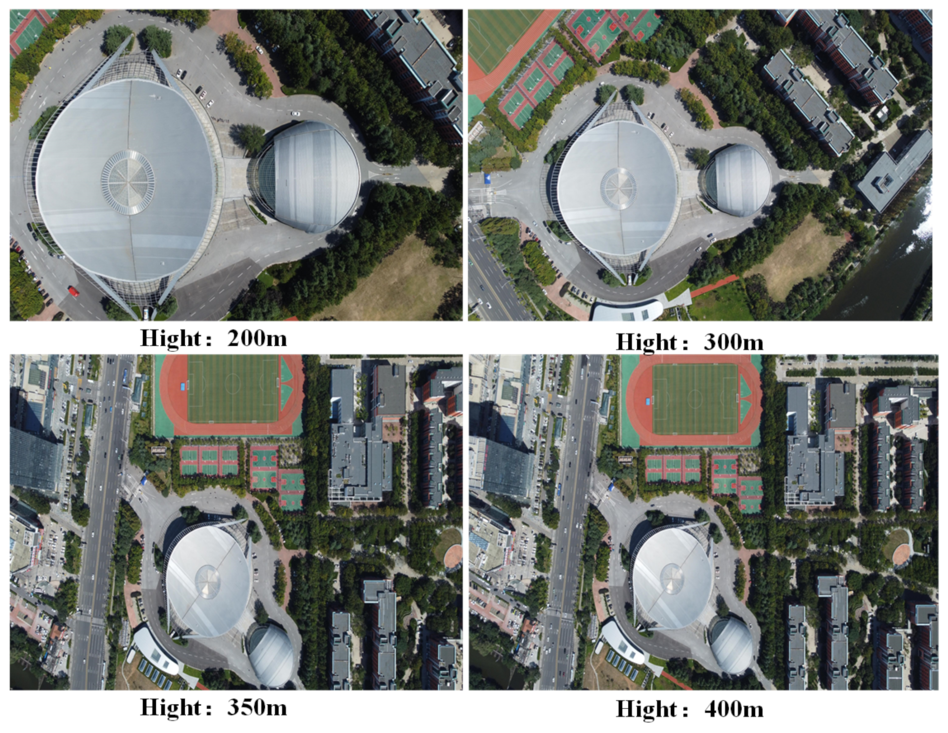
| Height (m) | Matching Points | Matching Accuracy (%) | Matching Error (m) |
|---|---|---|---|
| 200 | 34 | 88.24 | 3.12 |
| 300 | 44 | 93.18 | 4.90 |
| 350 | 39 | 89.74 | 3.12 |
| 400 | 33 | 90.91 | 4.98 |
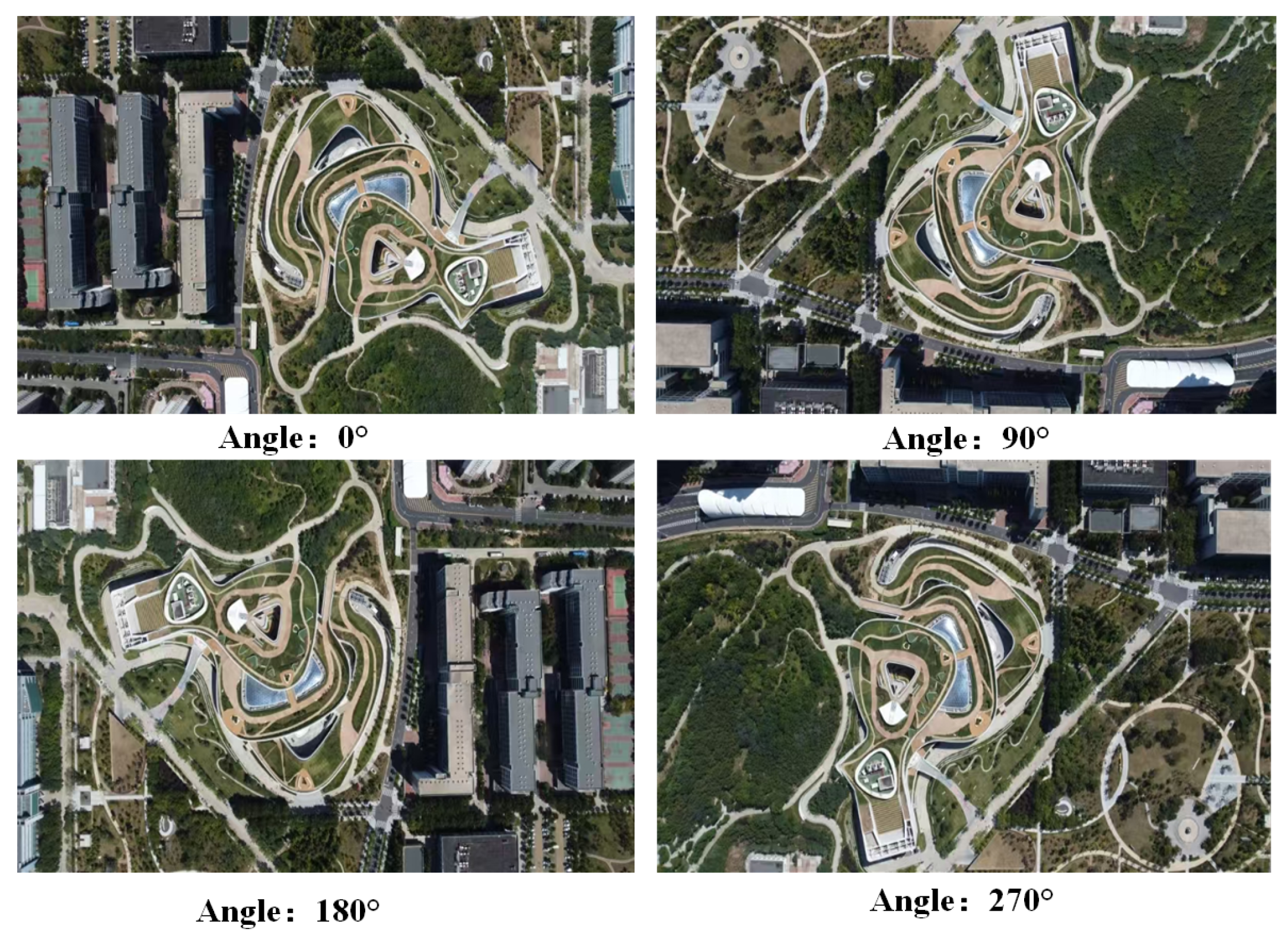
| Angle (°) | Matching Points | Matching Accuracy (%) | Matching Error (m) |
|---|---|---|---|
| 0 | 72 | 94.44 | 4.22 |
| 90 | 63 | 90.48 | 3.53 |
| 180 | 71 | 91.55 | 4.22 |
| 270 | 65 | 92.31 | 5.23 |
| Network | FLOPs (GB) | Memory Usage (MB) | Model Size (MB) | Processing Time (s) | Robustness (%) |
|---|---|---|---|---|---|
| shuffleNet V2 [44] | 0.14 | 90 | 8 | 3.65 | 78% |
| MobileNetV3 [45] | 0.21 | 100 | 12 | 3.78 | 89% |
| BlazeFace [46] | 0.30 | 60 | 1.8 | 1.25 | 49% |
| GhostNet [47] | 0.29 | 110 | 19 | 4.98 | 72% |
| EnvNet-Lite (ours) 1* | 0.17 | 85 | 5.6 | 2.89 | 93% |
| Modular Assembly | Positioning Accuracy (%) | Matching Accuracy (%) | Robustness (%) |
|---|---|---|---|
| LFE | 77.77 | 69.54 | 76 |
| EnvNet-Lite-EAAM | 78.72 | 72.04 | 72 |
| EnvNet-Lite | 79.09 | 72.21 | 84 |
| LFE+EnvNet-Lite | 79.16 | 73.12 | 85 |
| FIM-JFF (ours) | 92.73 | 85.33 | 91 |
Disclaimer/Publisher’s Note: The statements, opinions and data contained in all publications are solely those of the individual author(s) and contributor(s) and not of MDPI and/or the editor(s). MDPI and/or the editor(s) disclaim responsibility for any injury to people or property resulting from any ideas, methods, instructions or products referred to in the content. |
© 2025 by the authors. Licensee MDPI, Basel, Switzerland. This article is an open access article distributed under the terms and conditions of the Creative Commons Attribution (CC BY) license (https://creativecommons.org/licenses/by/4.0/).
Share and Cite
Gong, F.; Hao, J.; Du, C.; Wang, H.; Zhao, Y.; Yu, Y.; Ji, X. FIM-JFF: Lightweight and Fine-Grained Visual UAV Localization Algorithms in Complex Urban Electromagnetic Environments. Information 2025, 16, 452. https://doi.org/10.3390/info16060452
Gong F, Hao J, Du C, Wang H, Zhao Y, Yu Y, Ji X. FIM-JFF: Lightweight and Fine-Grained Visual UAV Localization Algorithms in Complex Urban Electromagnetic Environments. Information. 2025; 16(6):452. https://doi.org/10.3390/info16060452
Chicago/Turabian StyleGong, Faming, Junjie Hao, Chengze Du, Hao Wang, Yanpu Zhao, Yi Yu, and Xiaofeng Ji. 2025. "FIM-JFF: Lightweight and Fine-Grained Visual UAV Localization Algorithms in Complex Urban Electromagnetic Environments" Information 16, no. 6: 452. https://doi.org/10.3390/info16060452
APA StyleGong, F., Hao, J., Du, C., Wang, H., Zhao, Y., Yu, Y., & Ji, X. (2025). FIM-JFF: Lightweight and Fine-Grained Visual UAV Localization Algorithms in Complex Urban Electromagnetic Environments. Information, 16(6), 452. https://doi.org/10.3390/info16060452