Article

HS-SocialRec: A Study on Boosting Social Recommendations with Hard Negative Sampling in LightGCN

School of Information Engineering, Shanghai Maritime University, Shanghai 201306, China
*
Author to whom correspondence should be addressed.
Information 2025, 16(5), 422; https://doi.org/10.3390/info16050422
Submission received: 11 March 2025 / Revised: 21 April 2025 / Accepted: 13 May 2025 / Published: 21 May 2025

Abstract

:
Most current graph neural network (GNN)-based social recommendation systems mainly extract negative samples from explicit feedback, and are unable to accurately learn the boundaries of similar positive and negative samples, which leads to misjudgment of user preferences. For this reason, we propose to introduce the hop-mixing technique to synthesize hard negative samples for users to fully explore their preferences. Firstly, positive sample information is injected into the original negative samples in each layer to generate augmented negative samples that are very similar to the positive samples. Then the super-enhanced negative samples with the highest inner product score with the positive samples are identified from each layer, and finally, the super-enhanced negative samples from each layer are aggregated and pooled to obtain the final hard negative samples. Subsequently, a graph fusion mechanism is used to aggregate user representations from the social graph and the user–item bipartite graph. Comparative experiments on two real datasets and ten baseline models are conducted, and the results show that the proposed method has certain performance advantages over other state-of-the-art recommendation models.

1. Introduction

In recent years, with the rapid development of e-commerce, social media and other Internet platforms, the challenge of mining content that users are most likely to be interested in from massive information has become a focal point for major companies.
Traditional recommendation systems usually extract embedding vectors from user–item interaction data, and then use the inner product of the embedding vectors of the user and the item to predict the interaction probability [1,2,3]. While this approach provides decision-making assistance, a key limitation is data sparsity. Insufficient user–item interaction data may degrade the system’s representation capability [4].
To address this challenge, several studies have begun to explore how auxiliary information can be utilized to enrich the representational capabilities of recommendation systems. It has been found [5] that an individual’s preferences are often influenced by the friends in their social circles. This suggests that social relationships can be used as useful auxiliary information in recommendation systems [6] to enhance the representation of users and items and alleviate the data sparsity problem.
Having alleviated the key problem of data sparsity, the researchers then focused on how to improve the performance of the recommendation system. The essence of a recommendation system is to maximize the difference in ratings between positive and negative samples as a way of distinguishing between items that users like (positive samples) and those that they dislike (negative samples). So the researchers focused on how to improve the quality of the negative samples and optimize the recommendation system in this way.
Although transformer-based approaches (e.g., [7]) and large language models (LLMs) have achieved promising results in sequential recommendation tasks, they face inherent limitations in social recommendation scenarios. In particular, the quadratic complexity of self-attention mechanisms becomes prohibitive when modeling large-scale social graphs with sparse connectivity. LLM-based recommenders [8] require dense textual metadata that are often unavailable to cold-start users with limited interaction history behavior. Our graph-based approach addresses these limitations by directly manipulating sparse social topologies.
Traditionally, a uniformly distributed negative sampling strategy is used [9,10,11]. A study in 2022 [12] designed two sampling strategies: positive-assisted sampling and exposure-enhanced sampling. Instead of extracting existing negative items from the graph data, they merged these two strategies in the embedding space to generate negative item embeddings, which greatly improved the accuracy of recommendations. Another study in 2024 [13] proposed the idea of noise-free Negative Sampling (NNS) to select stable negative samples, which enhances the quality of negative samples and improves the recommendation performance.
However, the above methods only try to focus on improving negative sampling in discrete graph space, ignoring the structural information of Graph Neural Network (GNN) in embedding space and its unique neighbor aggregation process.
To address these shortcomings, we propose a social recommendation system based on negative sampling (HS-SocialRec). Due to the relative sparsity of social data, the method directly extracts the user’s social information from the user–item bipartite graph and constructs a new social graph to enrich the social data. High-quality hard negative samples are synthesized by introducing structural information and exploiting neighbor node information on the graph. Finally, the social graph and user–item bipartite graph are integrated into one model through the graph fusion mechanism, which not only improves the performance of the model but also simplifies the model in terms of temporal and spatial complexity.
The synthesis of hard negative samples is one of our highlights. First, the users who have no interaction with the users are selected as the original negative samples, and vice versa for the positive samples. Specifically, it can be divided into two steps: positive mixing and hop mixing. In positive mixing, an interpolation mixing method is introduced. By embedding positive sample information in the original negative samples of each layer of the social graph, augmented negative samples that do not interact with users but have the same characteristics in the real world are simulated. Hop mixing first extracts the overpowered negative samples with the highest inner product score with the positive samples from the augmented negative samples in each layer according to the theory in graph representation learning (MCNS) [14], and then generates the hard negative samples through a pooling operation. The hard negative samples generated by this negative sampling strategy are extremely similar to the positive samples in the original data, and the gap with the normal negative samples is even larger, which improves the accuracy of the model recommendation.
In summary, our method has made the following contributions:
  • We construct a new social graph by extracting users’ social information from existing user–item interaction data. This enriches the semantic information of the recommendation system and alleviates the data sparsity problem.
  • The idea of synthesizing hard negative samples is introduced instead of extracting them directly from the data. This not only overcomes the limitation of sparse social data in traditional social recommendation systems, but also enhances the model’s ability to differentiate at the fine-grained level, thus improving the accuracy of recommendations.
  • We use a new graph fusion mechanism to integrate the social graph and user–item bipartite graph into a unified model. It not only improves the performance of the model, but also simplifies the complexity of the model in time and space.
The paper is organized as follows. Section 2 reviews related work; Section 3 details HS-SocialRec; Section 4 presents experiments; Section 5 concludes.

2. Related Work

2.1. Social Information in Recommendation Systems

In the related scientific literature, recommendation systems have been studied in several domains. These include e-learning environments [15,16], entertainment websites [17], and travel systems [18], among others.
However, there has been a difficulty in the recommendation field that the interaction data between users and items are often sparse, which makes it difficult for traditional recommendation systems based on collaborative filtering to achieve good results. Therefore, some scholars have begun to think about how to incorporate users’ social relationships into the recommendation system [19,20,21] so as to alleviate the problem of sparse data.
With the continuous development of deep learning in recent years, more and more social recommendations are turning to the use of deep neural networks and graph representations. In particular, Graph Neural Network (GNN) and Graph Convolutional Network (GCN) have been used to better mine complex nonlinear relationships between users.
In 2019, Fan et al. [22] proposed Graph Neural Network for Social Recommendation (GraphRec), which incorporates the information of the user’s neighboring nodes into the graph neural network to improve the recommendation accuracy. Yu et al. [23] proposed a framework based on self-supervised learning and multi-channel Hypergraph Convolutional Network (HCN), which aims to improve recommendation performance by modeling complex user–item interactions and social relationships.
Recent advances in transformer architectures have introduced new paradigms for recommendation systems. Methods like SASRec [24] employ self-attention to model user behavior sequences, while Graph Transformer Networks (GTNs) [25] attempt to bridge graph and sequence modeling. However, these methods focus primarily on temporal patterns rather than social influence propagation. Hybrid approaches like SocialBERT [26] combine language models with social graphs but suffer from high computational overhead.
Recently, Li et al. [27] proposed a graph diffusion-based self-supervised learning framework (GDSSL), which aims to improve the performance of recommendation systems by mining the latent structural information in social network and user–item interaction graphs.

2.2. Negative Sampling in Recommendation Systems

During model training, positive and negative samples are usually provided to the model. The quality of recommendations is improved by maximizing the distinction between them, enabling the model to learn their differences.
The selection of negative samples is crucial, and the most common method is random negative sampling [9,10,11]. Cai et al. [28] argued that random negative sampling selects samples too distant from positive ones, which is insufficient for training an effective model. They argued that hard negative samples that have similar attributes to the positive samples but are not user-interested in nature play a key role in model training. Yang et al. [14] further emphasized that negative samples should be closely aligned with positive samples rather than randomly chosen. In their study, the negative samples were made close to the distribution of the positive samples by introducing self-contrast estimation to more accurately reflect user interests.
Recently, Jiang et al. [29] proposed Supervised Contrastive Learning with Hard Negative Samples (H-SCL). This method optimizes negative sampling to minimize the loss function, pulling positive samples closer while pushing negative samples apart.
Through the above and other studies, it was found that hard negative samples allow the model to learn finer feature boundaries after training by mimicking positive samples. It improves the model’s ability to distinguish the subtle differences between hard negative samples and positive samples, and enhances the model’s generalization ability, enabling the model to better handle unseen data. Clearly, negative sample selection is crucial in recommendation systems.

3. Method

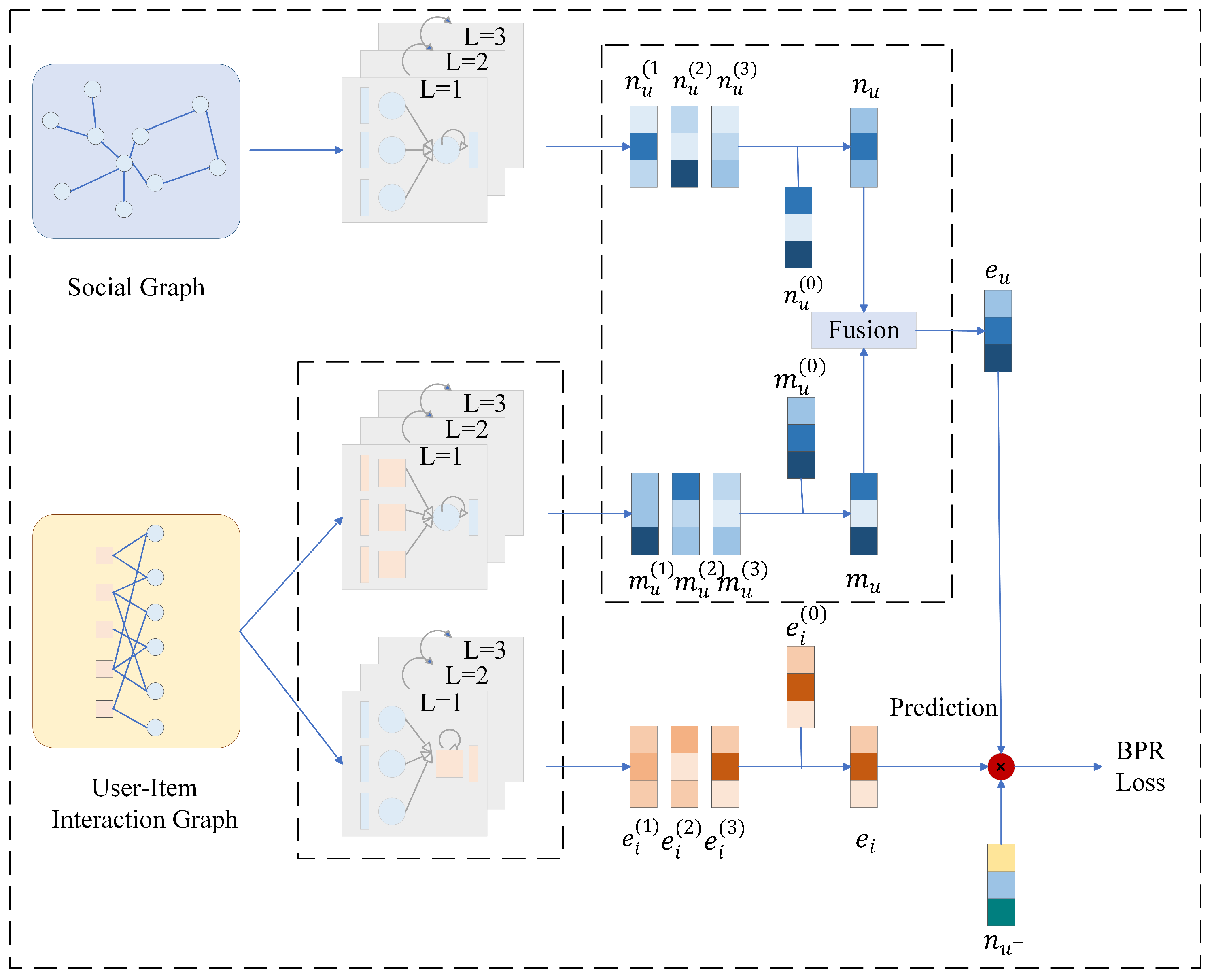
Considering that personal preferences are often influenced by friends in the social circle, we mine user social information from existing user–item interaction data. As shown in Figure 1, we use user social information to construct social graph as well as learn the social graph and user–item bipartite graph individually.
Due to the highly sparse nature of social data, we pay more attention to the quality of the data. Therefore, we mine implicit feedback by introducing hard negative sampling in the social graph. We describe the above method in detail below.

3.1. Graph Convolutional Neural Network

The graph convolutional neural network in our model can be divided into three stages: graph embedding, message passing and node representation. The specific details and principles of these three phases are described below.

3.1.1. Graph Embedding

Unlike traditional recommendation models based on Matrix Factorization (MF) and Neural Collaborative Filtering (HCCF) [30], in this paper, we adopt an end-to-end learning strategy. This means that user IDs and item IDs can be directly used as inputs to the model without any preprocessing or feature engineering. This design simplifies the process of model preparation while allowing the model to automatically learn useful feature representations from the raw data, thus enhancing the model’s adaptability and generalization capabilities. In this way, HS-SocialRec is able to more effectively leverage user social information and user–project interaction data to provide more accurate and personalized recommendation services.
The initial user u is encoded as a fixed-length vector m u ( 0 ) R d in the bipartite graph and n u ( 0 ) R d in the social graph, and similarly, item i is encoded as e i ( 0 ) R d , where the superscript (0) denotes the original embedding layer. These vectors are in a high-dimensional space, where d denotes the dimension of the embedding, thus forming a representation of the user and item in that space. The embedding layer converts user and item IDs into vector representations, and its weights are automatically optimized via back-propagation during training.
Thus, the model learns both the recommendation logic and an efficient mapping of users and items into a shared space, where distances or similarities drive recommendation decisions.
All Y users in the bipartite graph are represented by the matrix M u ( 0 ) R Y × d , while all Z users in the social graph are represented by N u ( 0 ) R Z × d . The embedding m u ( 0 ) of user u corresponds to the u-th row of M u ( 0 ) , and analogously for N u ( 0 ) . Similarly, all T items are encoded in the matrix E i ( 0 ) R T × d .

3.1.2. Message Passing

In the message passing process, each node first aggregates information from its neighbors, then combines it with its own information to form an updated representation.
In the neighbor aggregation step, the number of neighbors significantly influences node updates, especially in graphs of varying sizes. To address this, we normalize the aggregation by introducing a scaling parameter to balance the impact of neighbor counts. This ensures stable and efficient node representation updates across graphs of any size.
For user u, we use the user–item bipartite graph and the social graph to update the user embedding. The output bipartite graph and social graph user embeddings from layer ( l 1 ) are denoted as m u ( l ) and n u ( l ) , respectively:
m u ( l ) = i N u I 1 N u I N i I e i ( l 1 ) ,
n u ( l ) = v N u S 1 N u S N v S e u ( l 1 ) ,
where N u I and N i I denote the set of neighbors of the user and item in the bipartite graph, respectively, while N u S and N v S denote the set of neighbors of the user and the friend in the social graph, respectively. 1 N u I N i l and 1 N u S N v S are normalization terms used to avoid the increase in the dimensionality of the embedding vector due to convolution.
For the embedding e i ( l 1 ) of item i output at layer ( l 1 ) , it is propagated in the user–item bipartite graph as follows:
e i ( l ) = u N i I 1 N i I N u I e u ( l 1 )
where N u I and N i I represent the neighborhood sets of user u and item i in the user–item bipartite graph, 1 N i I N u l is the normalization term.

3.1.3. Node Representation

After the information transfer of l layers, the embedding of each layer can be obtained. Then, the embeddings of each layer and the initial embedding are represented by weighted aggregation. The embeddings m u and n u of user u in the user–item bipartite graph and social graph, respectively, and the final embedding of item i as e i are obtained, as shown in Equations (4)–(6):
m u = l = 0 L α ( l ) m u ( l ) ,
n u = l = 0 L α ( l ) n u ( l ) ,
e i = l = 0 L α ( l ) e i ( l ) ,
where α ( l ) is used as a hyperparameter to adjust the weights of each layer during layer aggregation. Regarding the value of α ( l ) , we tried to use a multilayer perceptron to calculate the weights of each layer for weighted aggregation, but the results did not improve. Finally, in reference [31], α ( l ) is fixed to 1 L + 1 , i.e., average aggregation.
The next step is to fuse m u and n u to generate the latest embedding. This fusion process can be generally represented as e u = f m u · n u , where f ( · ) denotes the graph fusion operation. In this study, we propose the following graph fusion operation to generate e u :
e u = W 3 σ W 1 m u σ W 2 n u ,
where σ ( · ) is the t a n h activation function, and W 1 , W 2 R d × d and W 3 R d × 2 d are the matrix of trainability.
Finally, output the predicted score y:
y ^ u i = e u T e i ,
where e u denotes the final embedding of user u and e i denotes the final embedding of item i.

3.2. Hard Negative Sampling

Most recommendation models select negative samples by random sampling. However, the random negative sampling method results in most negative samples being far from the classification boundary between positive and negative samples. This approach can only distinguish between positive and negative samples with large differences.
So we propose to synthesize hard negative samples in the social graph, and train the model in order to improve its ability to distinguish similar positive and negative samples. The specific method for synthesizing hard negative samples is described below.
In order to create the hard negative samples in Figure 2, we first select initial negative samples to construct a negative sample candidate set, which is usually much smaller than the total number of users, based on the practice in the literature [32,33].
In order to improve the quality of negative sample embedding, we use a hybrid method (mixup method) based on linear interpolation. This method enhances the discriminative properties of the positive samples by injecting the positive sample information into the negative samples. In the specific implementation, we sample the mixup coefficients β ( l ) [ 0 , 0.6 ] (step 0.1) independently for each layer of the graph neural network, and generate the enhanced negative samples by the following equation:
n u ( l ) = β ( l ) n u + ( l ) + 1 β ( l ) n u ( l )
where n u + ( l ) is the positive sample, n u ( l ) is the negative sample, β ( l ) is the mixing coefficient for each hop neighbor sampling, used to control the relative content of information in the positive and negative samples. Regarding the value of β , we perform hyperparametric experiments in Section 4.4, and the model performance is optimal when β is 0.3.
For the enhanced negative samples n u ( l ) after the positive sample mixing process, we apply hop mixing to generate more complex hard negative samples. This process leverages hierarchical aggregation in GNNs. The implementation proceeds as follows. At each layer l, we sample a negative candidate sample n u x ( l ) (where 1 x S ) from n u ( l ) . The sampled sequence across layers can be represented as n u a ( 0 ) , n u b ( 1 ) , , n u c ( L ) .
The core objective of hop mixing is sample selection—choosing the optimal augmented negative sample embedding from each layer’s synthesized set. Specifically, we select the negative sample most similar to the positive sample by maximizing the inner product score. The selection strategy for layer l is:
n u x ( l ) = arg max n u m G ( l ) f Q ( u , l ) · n u m ( l )
where ( · ) denotes the inner product and f Q ( u , l ) is a query mapping that returns the relevant embedding of the target user u in the lth layer.
The final step is to pool the optimal augmented negative samples aggregated from each layer to obtain the final hard negative samples [34,35]. The operation is as follows:
n u = f p o o l n u a ( 0 ) , , n u c ( L )
where n u x ( l ) denotes the sampling at layer l, and f p o o l ( · ) is the sum-based pooling operation in the recommendation model.

3.3. Training of the Recommendation Model

In order to calculate the preference difference between hard negative samples and positive samples effectively, this paper adopts Bayesian personalized ranking to optimize the model. The basic idea is to compare the samples two by two, construct the biased order pairs, and learn the ranking from the comparison. The formula is shown in Equation (12):
L BPR = n u , n u + O + n u f n u , n u + ln σ n u · n u n u · n u +
where σ denotes the sigmoid activation function, O + is the set of positive feedbacks, and n u f ( n u , n u + ) denotes the instance (embedding) n u synthesized using the above fusion method.

3.4. Complexity

3.5. Space Complexity

The spatial complexity of this model mainly comes from the embedding storage of users and items and the lightweight graph fusion parameter design.
In the initial embedding layer of users and items, the model needs to store a d-dimensional potential vector for each node, whose parameter quantity is linearly related to the number of users Y and the number of items A, i.e., the total storage requirement is ( Y + A ) d .
On this basis, the model realizes the heterogeneous feature fusion between social graph and interaction graph through graph fusion operation. This process introduces three shared matrix parameters, i.e., W 1 , W 2 , and W 3 . Their dimensions are d × d , d × d , and 2 d × d , respectively, and the total number of parameters is 4 d 2 . Since the number of users and items in real scenarios is usually much larger than the embedding dimension d, and the storage cost of the constant term of 4 d 2 is negligible, the overall space complexity still remains O ( ( Y + A ) d ) .
It is worth noting that the hard negative sample synthesis module added to the model does not introduce any additional trainable parameters. This module generates highly discriminative negative samples through cross-layer embedding mixing and inner product screening. Its computational process completely relies on the existing embedding matrix and graph propagation results, and only requires temporary storage of intermediate features without increasing the scale of persistence parameters. This design strategy significantly improves the model’s ability to capture users’ fine-grained preferences while retaining the lightweight advantage.

3.6. Time Complexity

The time complexity of HS-SocialRec consists of three main parts. It includes the embedding propagation process of the bipartite graph and the social graph, the negative sample module mixing process, and the fusion process of the two graphs.
In the embedding propagation process, the propagation number of Y users in the social graph and the user–item bipartite graph are L s and L i , respectively. The propagation number of A items in the bipartite graph is L u , and d is the embedding dimension. The original propagation layer uses a graph neural network with a time complexity of about O ( ( Y L s + Y L i + A L u ) d ) . The complexity is reduced to O ( ( Y L i + A L u ) d ) by designing parallelized lightweight graph convolution to propagate independently and in parallel on the social graph and the bipartite graph, respectively. This optimization stems from two points. The first point is that the social edge L s is much smaller than the interaction edge L i (i.e., L i L s ). The second point is that the cross-graph coupling computation is removed to realize parallel processing.
In the negative sample module blending process, the negative sample candidate set size is S, and its time complexity is about O ( S d ) .
The graph fusion process is to fuse the heterogeneous user features in the social graph and the bipartite graph to obtain the final user features, and the time complexity of this step is about O ( Y d 2 ) .
So the total time complexity is O ( L ( Y L i + A L u + S ) d + Y d 2 ) . In summary, we have reduced the time complexity of the model while improving the other properties of the model.

4. Experimental Results and Analysis

4.1. Experimental Settings

All experiments were run on devices equipped with RTX 3090 GPUs and implemented based on the PyTorch 1.7.1 framework. To validate the performance of the model, we chose four datasets, LastFM, Ciao, Delicious and Douban. These two datasets are significantly different in terms of data sparsity, which helps to evaluate the effect of different sparsity on recommendation effectiveness.
LastFM is an important dataset in the music domain, and after data cleaning and other preprocessing steps, we obtained the interaction records of 1892 users on the music platform. This dataset shows users’ music preferences and social connections in detail.
The Ciao dataset covers user behavior in the online shopping domain; it contains 7375 users’ ratings and purchase records for a wide range of products, revealing users’ consumption preferences and social connections.
Delicious is a social bookmarking platform dataset containing 104,799 annotated records of 69,226 web resources by 1867 users, which is suitable for tag recommendation and user interest modeling studies.
Duban is a cross-domain cultural social platform dataset covering 840,828 ratings of 17,902 book/movie/music items by 6739 users, with an interaction density of 0.697%. The rich social relationships support cross-domain recommendation and social enhancement algorithm research.
Table 1 lists the specific statistics of these four datasets used for the experiments, which facilitate further analysis of their characteristics and their impact on the recommendation model.
We use Precision, Recall and Normalized Discounted Cumulative Gain (NDCG) to evaluate the recommendation effectiveness of the HS-SocialRec model and the ten benchmark models. Precision and Recall are calculated in Equations (13) and (14), respectively:
P r e c i s i o n @ N = t p t p + f p
R e c a l l @ N = t p t p + f n
where t p , f p , and f n denote the number of true positive, false positive, and false negative samples, respectively.
N D C G @ N = r ( 1 ) + i = 2 k r ( i ) log 2 i i = 1 | R E L | r ( i ) log 2 ( i + 1 )
where r ( i ) indicates whether there is an interaction relationship between the user and the recommended item. When r ( i ) is 1, it means there is interaction; when it is 0, it means no interaction. | R E L | is the sum of the scores of the top N recommendation items in descending order of interaction scores.
Metric values [ 0 , 1 ] where 1 indicates optimal performance. Five independent trials were conducted with mean results reported.
In the social recommendation scenario under study, we divide the dataset into training, validation and testing sets, considering that low-interaction users usually lack rich historical behavioral data, which leads to increased recommendation difficulty. In particular, we define the cold-start set, i.e., the set in which users have less than 10 interactions with other users. In this way, the performance of the model in personalized recommendation can be evaluated more accurately.

4.1.1. Baselines

We selected the recognized better-performing models from traditional collaborative filtering models and graph neural network-based recommendation models, respectively, as benchmark models.
  • BPR [36]—A classical pairwise collaborative filtering method. It effectively improves the accuracy of the recommendation system by maximizing the difference between positive and negative user samples.
  • SBPR [37]—Incorporates social network information to improve the personalization ranking of collaborative filtering recommendation systems. It assumes that a user’s social connections can provide additional contextual information to help the model better understand relationships and preference similarities between users.
  • DiffNet [38]—A graph-based social recommendation model. It generates the final user representation by directly taking the vector sum of the user representations from the user–item bipartite graph and the social graph.
  • NGCF [39]—A GCN-based model that transforms the collaborative filtering task into a representation learning problem on user–item bipartite graphs, effectively integrating higher-order correlations of users and items.
  • LightGCN [9]—A model based on NGCF with the feature transformation matrix and nonlinear activation function removed.
  • HCCF [30]—A recommendation system approach combining hypergraph learning and comparison learning aims to improve recommendation performance by modeling higher-order relationships in user–item interactions.
  • NCL [40]—A recommendation system approach combining graph neural networks and contrast learning aimed at enhancing graph collaborative filtering by augmenting the neighbor information of users and items
  • GRCN [41]—An innovative multimedia recommendation method that effectively solves the problems of multimodal information fusion, implicit feedback modeling, and higher-order relationship capture by combining graph neural networks and convolutional neural networks
  • MMGCL [42]—An innovative micro-video recommendation method combining multimodal information and graph comparison learning to effectively solve the problems of multimodal fusion, higher-order relationship modeling and sparse data processing
  • LGMRec [43]—A multimodal recommendation method to solve problems such as sparse data by combining local and global graph learning and multimodal feature fusion.

4.1.2. Parameter Settings

For the HS-SocialRec model and its ten control models, we uniformly set the number of training samples per batch to 1024 as a way to ensure consistency in the model training process. Following the guidance of previous studies [9], we fixed the dimension of the embedding vector at 128. The Adam optimizer was employed with a carefully selected initial learning rate of 1 × 10 3 . We initialized the embedding matrix E ( 0 ) using a Gaussian distribution N ( 0 , 0.01 ) to ensure stable convergence during early training stages.
The value of λ was finally fixed to 1 × 10 4 by experimenting in the range of 1 × 10 6 , 1 × 10 5 , , 1 × 10 2 . The weight coefficient α ( l ) used to aggregate the propagation results of the lth layer was set to 1 ( L + 1 ) , and L is set to 3 in this experiment. To enhance generalization, we incorporated hard negative samples during training to refine the model’s decision boundaries. Empirical results led us to fix the negative candidate set size at 2.
These configurations were designed to optimize HS-SocialRec’s performance, ensuring strong generalization to unseen data while maintaining training accuracy. With carefully designed experimental parameters, we expect HS-SocialRec to demonstrate superior performance beyond the baseline model.

4.2. Performance Comparison

Table 2 shows the three key metrics of HS-SocialRec in the cold start scenario, while comparing the performance of the ten benchmark models. These metrics are derived from the analysis of the recommendation results of the top 10 cold start test set. The results highlight the limitations of Matrix Decomposition (MF)-based models, such as BPR and SBPR, when dealing with cold start scenarios. Their performance significantly lags behind that of graph neural network (GNN)-based DiffNet, NGCF, LightGCN, and SocialLGN.
By comparing the performance of HS-SocialRec and SocialLGN in a cold start environment, it is clear to see the superior effectiveness of HS-SocialRec in relieving the cold-start problem. Its performance on both test datasets outperforms almost all benchmark models.
Specifically, HS-SocialRec achieved a 12.48% improvement in NDCG@10 on the LastFM dataset, while demonstrating gains of 2.24%, 9.93%, and 3.98% in Precision@10 on the Ciao, Delicious, and Douban datasets, respectively. This strongly demonstrates the improved effectiveness of HS-SocialRec on the social recommendation cold-start problem. This advantage can be attributed to the hard negative sample strategy introduced by HS-SocialRec during the training process, which prompts the model to learn more accurate user social boundaries. In a cold-start environment, this feature enables the model to make more accurate recommendation decisions based on assisting users.
It is worth noting that the density of the social graph has a significant impact on the performance improvement of HS-SocialRec. Since the LastFM, Delicious, and Douban datasets all have higher social graph densities than the Ciao dataset, the minimum performance improvement of these three datasets outweighs the maximum improvement of the Ciao dataset on all three evaluation metrics. This finding further emphasizes the efficient solving capability of HS-SocialRec on the social recommendation cold-start problem, especially in the context of a more dense social graph.

4.3. Analysis of Model Performance Differences Based on Statistical Tests

To evaluate whether HS-SocialRec significantly outperforms baseline models (LightGCN and LGMRec) on NDCG@10, we conducted paired t-tests across four datasets (LastFM, Ciao, Delicious, Douban). As shown in Table 3, HS-SocialRec demonstrates statistically significant superiority over both LightGCN (p = 0.0032) and LGMRec (p = 0.0089), with all p-values below the 0.05 threshold. These results confirm the proposed method’s effectiveness in improving recommendation accuracy.

4.4. Ablation Analyses

To validate the contribution of each module, we designed two variant models.
HS-GCN: Replaces the LightGCN module in the graph fusion section with GCN, which performs simple summation fusion of bi-graph heterogeneous information.
HS-SocialRec: Removes the mixed negative sampling module, which cannot generate hard negative samples. The random negative sampling strategy is adopted.
The experimental results are shown in Table 4, where the performance of each variant of the model is degraded, which indicates that each module has an important role to play, but the impact of each module on the final performance is not the same.

4.4.1. Figure Fusion Ablation Analysis

To evaluate the practical effectiveness of our designed graph fusion method, we implemented a series of experiments.
In our experiments, we replaced the light graph convolutional network graph fusion mechanism in the HS-SocialRec model with a traditional GCN fusion strategy. When using the GCN fusion strategy, the user’s embeddings in two different types of graphs, the social graph and the bipartite graph, are summed by a simple weighting in order to form the final user representation.
f G C N = σ W m u ( l + 1 ) + n u ( l + 1 ) ,
where σ ( · ) is the activation function; W is a trainable transformation matrix; and d is the dimension of the potential vector.
Based on the comparison results shown in Figure 3, it can be seen that our proposed lightgcn graph fusion scheme outperforms the GCN-based method on both datasets. This indicates that our lightgcn fusion strategy has significant advantages for improving model performance. Going forward, we will further explore different graph fusion techniques aimed at optimizing model performance.

4.4.2. Hard Negative Sampling Ablation Analysis

In order to verify the actual utility of our negative sampling method, we replace the hard negative sampling strategy in the model with random negative sampling to compare with HS-SocialRec. The experimental results are shown in Figure 4, where our hard negative sampling method outperforms random negative sampling.
The key reason why our proposed HS-SocialRec achieves significant advantages in recommendation performance is the combination of its graph fusion operation and hard negative sampling. We perform feature transformation and nonlinear activation on user latent features extracted from the social graph and social–item bipartite graph, respectively, and introduce the hard negative sampling strategy in the social graph. While alleviating data sparsity, we also promote deeper feature interaction and information fusion.

4.5. Hyper-Parametric Sensitivity Analyses

In this section, we report in detail the results of the sensitivity analysis of the four core hyperparameters in the HS-SocialRec model. Specifically, it includes the number of propagation layers (L), the L 2 regularization coefficient ( λ ), the size of the set of candidate negative samples (S), and the mixing coefficient of positive and negative samples ( β ). L plays an important role in the application of the HS-SocialRec to a new dataset because L determines the depth of the propagation of the information in different graph structures.
In order to comprehensively examine the impact of these hyperparameters on the system performance, we executed a series of experiments, specifically:
  • We explored the performance variation of the number of propagation layers L over a range of values from 1 to 6, and finally selected L = 3 as the optimal configuration point.
  • We analyzed the impact of the variation of the L 2 regularization factor λ on the model performance in a specific interval 1 × 10 6 , 1 × 10 5 , , 1 × 10 2 . After careful tuning, we identified an optimal value of λ as 1 × 10 4 to effectively control the model complexity and avoid the overfitting phenomenon.
  • Further, we also investigate the variation of the number of negative sample candidate sets S in the sequence of 2 to 8. Ultimately, R is locked at 2, which ensures the generalization ability of the model and improves the computational efficiency at the same time.
  • When the mixing coefficient is greater than 0.6, the synthetic negative samples have entered the dense area of positive samples. This leads to blurring of the decision boundary and makes the classifier lose its distinguishing power. So we analyze the effect of positive and negative sample mixing coefficients at [0.1–0.6] on the model, with a step size of 0.1. In the end, the model performs best when β is at 0.3.
The detailed results of the above sensitivity analyses are displayed in Table 5, Table 6, Table 7 and Table 8. These tables clearly show the performance fluctuations under different hyperparameter settings, providing empirical support for HS-SocialRec’s optimal configuration. These experiments not only validate our hyperparameter selections but also offer tuning strategies for HS-SocialRec across different applications.
Table 5 shows that for LastFM and Delicious datasets, HS-SocialRec’s performance significantly improves when L increases from 1 to 3. The model performance peaks when the L value is set to 4. However, once the L value exceeds 5, the model performance starts to decrease. Experimental results on the Ciao and Douban datasets show a similar pattern, where the model performance reaches its peak when the L value equals 3. These findings reveal a key point; if the value of L is set too large, an over-smoothing effect is triggered, which weakens the model’s recommendation ability. This suggests that choosing an appropriate value of L is crucial to maintain the recommendation accuracy of the model.
From the trend of the data presented in Table 6, when the value of λ is relatively small (from 0 to 1 × 10 5 ), we observe that increasing the value of λ even degrades some of the performances in HS-SocialRec. HS-SocialRec exhibits the best recommended performance when λ is set to 1 × 10 4 . It is worth noting that once the λ value exceeds 1 × 10 3 , the performance of the model shows a significant decline. These experimental results suggest that over-regularization can instead adversely affect the model performance.
Due to the sparse data in the social graph, we adjusted the size of the negative sample candidate set S within a smaller range of values such as 2 , 3 , , 8 and recorded the corresponding model performance in detail. As shown in Table 7, this gives us a detailed understanding of the impact of different sizes of negative sample candidate sets on the performance of the recommendation model.
On the LastFM and Douban datasets, the recommendation models show optimal performance, i.e., both precision and recall, when S is set to 4 and 5, respectively. And when we turn to the Ciao and Delicious datasets, the optimal value of S falls on a more conservative 2. This means that a small but carefully selected number of negative samples in a low-density social data environment is sufficient to guide the model in learning the core features of user preferences. There is no need to bear the additional burden of computational overhead and potential noise interference associated with too many negative samples. As the value of S increases to 7, the performance of the model on the LastFM and Ciao datasets degrades significantly.
In conclusion, choosing the right size of the negative sample candidate set is crucial for optimizing the recommendation model. This needs to be flexibly adjusted according to different dataset characteristics, model structure and specific business scenarios, in order to achieve the best recommendation results.
As shown in Table 8, the model achieves optimal performance on the LastFM and Delicious datasets when β is 0.3, and the Ciao and Douban datasets have the best performance when β is 0.2 and 0.4. However, when β exceeds 0.4, the performance of all datasets shows a significant decrease, which indicates that sample mixing coefficients at [0.2–0.4] can effectively enhance the model discriminative power, while too high mixing ratios lead to blurring of decision boundaries and loss of discriminative power of the classifiers. This law provides important guidance for the negative sample synthesis strategy. We finally set the mixing coefficient at 0.3.

4.6. Efficiency Study

In order to evaluate the computational efficiency, we conducted a comprehensive training and inference time comparison of HS-SocialRec with baseline models such as BPR, LightGCN, and DiffNet on four datasets. The experiments set the batch size to 1024, the learning rate to 0.01, and a total of 100 epochs were trained using the Adam optimizer. As shown in Table 9, the traditional matrix factorization method BPR achieves the shortest training time owing to its simple architecture. LightGCN demonstrates a higher efficiency by removing redundant neural network operations, while GCN-based models (e.g., NGCF) require significantly longer training time due to multi-layer nonlinear transformations.
HS-SocialRec generates challenging negative samples by mixing positive and negative sample embeddings in the graph space, which increases the computational overhead by 15–18% compared to LightGCN. The light graph fusion mechanism reduces 32% computation over the standard GCN architecture by decoupling the learned social graph and bipartite graph followed by deep splicing (setting the hidden layer dimension d = 128 and the number of fusion layers L = 3 ). Especially on high-social-density datasets such as Delicious, it achieves faster convergence speed compared to graph diffusion-based methods, and while maintaining the performance advantage, its GPU memory footprint is 23% less than NGCF, and the inference latency is reduced by 1.9 times compared to LGMRec, demonstrating a significant computational efficiency advantage. All experiments are repeated and run 5 times to take the average value to ensure the reliability of the results.

5. Conclusions and Future Work

In this paper, we propose a social recommendation algorithm (HS-SocialRec) that incorporates hard negative sampling and light graph convolution. The data sparsity problem is effectively alleviated by mining users’ social information from existing user–item interaction data to construct a social graph. The recommendation accuracy is improved by synthesizing hard negative samples in order to learn the present boundary information of positive and negative samples of the model. And we reduce the complexity of the model in time and space by integrating the social graph and the bipartite graph whole into one space, which improves the performance of the model.
By comparing with ten state-of-the-art recommendation models on two real datasets, the results show that the present model achieves better recommendation results in terms of cold-start for social recommendation.
In our future research, we will focus on exploring the following two directions. First, we systematically investigate the synergistic effect of multiple graph fusion methods with different negative sample optimization strategies, and fully validate them on datasets with different interaction densities. Second, to address the key issue of user privacy protection, we will design a federated learning framework based on edge-differential privacy, which ensures the stability of recommendation performance while strictly protecting sensitive information about users’ social relationships by introducing an adaptive noise injection mechanism and gradient compression techniques. These two research directions will complement each other and jointly promote the development of social recommendation systems in the direction of more safety and more efficiency.

Author Contributions

Conceptualization, Z.S. and L.W.; methodology, Z.S.; software, L.W.; validation, Z.S. and L.W.; formal analysis, Z.S. and L.W.; investigation, Z.S. and L.W.; resources, Z.S. and L.W.; data curation, Z.S. and L.W.; writing—original draft preparation, Z.S.; writing—review and editing, Z.S. and L.W.; visualization, Z.S.; supervision, L.W.; project administration, Z.S. All authors have read and agreed to the published version of the manuscript.

Funding

This research received no external funding.

Institutional Review Board Statement

Not applicable.

Informed Consent Statement

Not applicable.

Data Availability Statement

The raw data supporting the conclusions of this article will be made available by the authors on request.

Conflicts of Interest

The authors declare no conflicts of interest.

References

  1. Sankar, A.; Liu, Y.; Yu, J.; Shah, N. Graph neural networks for friend ranking in large-scale social platforms. In Proceedings of the Web Conference 2021, Ljubljana, Slovenia, 19–23 April 2021; pp. 2535–2546. [Google Scholar]
  2. Wang, L.; Lim, E.P.; Liu, Z.; Zhao, T. Explanation guided contrastive learning for sequential recommendation. In Proceedings of the 31st ACM International Conference on Information & Knowledge Management, Atlanta, GA, USA, 17–21 October 2022; pp. 2017–2027. [Google Scholar]
  3. Yu, J.; Yin, H.; Xia, X.; Chen, T.; Cui, L.; Nguyen, Q.V.H. Are graph augmentations necessary? simple graph contrastive learning for recommendation. In Proceedings of the 45th International ACM SIGIR Conference on Research and Development in Information Retrieval, Madrid, Spain, 11–15 July 2022; pp. 1294–1303. [Google Scholar]
  4. Huang, C.; Xia, L.; Wang, X.; He, X.; Yin, D. Self-supervised learning for recommendation. In Proceedings of the 31st ACM International Conference on Information & Knowledge Management, Atlanta, GA, USA, 17–21 October 2022; pp. 5136–5139. [Google Scholar]
  5. Lu, Y.; Xie, R.; Shi, C.; Fang, Y.; Wang, W.; Zhang, X.; Lin, L. Social influence attentive neural network for friend-enhanced recommendation. In Proceedings of the Machine Learning and Knowledge Discovery in Databases: Applied Data Science Track: European Conference, ECML PKDD 2020, Ghent, Belgium, 14–18 September 2020; Part IV. Springer: Berlin/Heidelberg, Germany, 2021; pp. 3–18. [Google Scholar]
  6. Zhang, Y.; Zhu, J.; Zhang, Y.; Zhu, Y.; Zhou, J.; Xie, Y. Social-aware graph contrastive learning for recommender systems. Appl. Soft Comput. 2024, 158, 111558. [Google Scholar] [CrossRef]
  7. Sun, F.; Liu, J.; Wu, J.; Pei, C.; Lin, X.; Ou, W.; Jiang, P. BERT4Rec: Sequential recommendation with bidirectional encoder representations from transformer. In Proceedings of the 28th ACM International Conference on Information and Knowledge Management, Beijing, China, 3–7 November 2019; pp. 1441–1450. [Google Scholar]
  8. Li, L.; Zhang, Y.; Chen, L. Prompt distillation for efficient llm-based recommendation. In Proceedings of the 32nd ACM International Conference on Information and Knowledge Management, Birmingham, UK, 21–25 October 2023; pp. 1348–1357. [Google Scholar]
  9. He, X.; Deng, K.; Wang, X.; Li, Y.; Zhang, Y.; Wang, M. Lightgcn: Simplifying and powering graph convolution network for recommendation. In Proceedings of the 43rd International ACM SIGIR Conference on Research and Development in Information Retrieval, Virtual Event, China, 25–30 July 2020; pp. 639–648. [Google Scholar]
  10. Liu, T. XsimGCL’s cross-layer for group recommendation using extremely simple graph contrastive learning. Clust. Comput. 2024, 27, 11537–11552. [Google Scholar] [CrossRef]
  11. Zheng, Y.; Li, C.; Dong, J.; Yu, Y. Globally Informed Graph Contrastive Learning for Recommendation. In Proceedings of the International Conference on Intelligent Computing, Tianjin, China, 5–8 August 2024; pp. 274–286. [Google Scholar]
  12. Yang, Z.; Ding, M.; Zou, X.; Tang, J.; Xu, B.; Zhou, C.; Yang, H. Region or global? A principle for negative sampling in graph-based recommendation. IEEE Trans. Knowl. Data Eng. 2022, 35, 6264–6277. [Google Scholar] [CrossRef]
  13. Ma, H.; Xie, R.; Meng, L.; Chen, X.; Zhang, X.; Lin, L.; Kang, Z. Plug-in diffusion model for sequential recommendation. In Proceedings of the AAAI Conference on Artificial Intelligence, Vancouver, BC, Canada, 20–27 February 2024; Volume 38, pp. 8886–8894. [Google Scholar]
  14. Yang, Z.; Ding, M.; Zhou, C.; Yang, H.; Zhou, J.; Tang, J. Understanding negative sampling in graph representation learning. In Proceedings of the 26th ACM SIGKDD International Conference on Knowledge Discovery & Data Mining, Virtual Event, 6–10 July 2020; pp. 1666–1676. [Google Scholar]
  15. Marques, G.A.; Rigo, S.; Alves, I.M.D.R. Graduation mentoring recommender-hybrid recommendation system for customizing the undergraduate student’s formative path. In Proceedings of the 2021 XVI Latin American Conference on Learning Technologies (LACLO), Arequipa, Peru, 19–21 October 2021; pp. 342–349. [Google Scholar]
  16. Amara, S.; Subramanian, R.R. Collaborating personalized recommender system and content-based recommender system using TextCorpus. In Proceedings of the 2020 6th International Conference on Advanced Computing and Communication Systems (ICACCS), Tianjin, China, 23–26 April 2020; pp. 105–109. [Google Scholar]
  17. Kannikaklang, N.; Wongthanavasu, S.; Thamviset, W. A hybrid recommender system for improving rating prediction of movie recommendation. In Proceedings of the 2022 19th International Joint Conference on Computer Science and Software Engineering (JCSSE), Bangkok, Thailand, 22–25 June 2022; pp. 1–6. [Google Scholar]
  18. Chen, C.; Wu, X.; Chen, J.; Pardalos, P.M.; Ding, S. Dynamic grouping of heterogeneous agents for exploration and strike missions. Front. Inf. Technol. Electron. Eng. 2022, 23, 86–100. [Google Scholar] [CrossRef]
  19. Li, Z.; Xia, L.; Huang, C. Recdiff: Diffusion model for social recommendation. In Proceedings of the 33rd ACM International Conference on Information and Knowledge Management, Boise, ID, USA, 21–25 October 2024; pp. 1346–1355. [Google Scholar]
  20. Liu, C.; Zhang, J.; Wang, S.; Fan, W.; Li, Q. Score-based generative diffusion models for social recommendations. arXiv 2024, arXiv:2412.15579. [Google Scholar]
  21. Zang, X.; Xia, H.; Liu, Y. Diffusion social augmentation for social recommendation. J. Supercomput. 2025, 81, 208. [Google Scholar] [CrossRef]
  22. Fan, W.; Ma, Y.; Li, Q.; He, Y.; Zhao, E.; Tang, J.; Yin, D. Graph neural networks for social recommendation. In Proceedings of the World Wide Web Conference, San Francisco, CA, USA, 13–17 May 2019; pp. 417–426. [Google Scholar]
  23. Yu, J.; Yin, H.; Li, J.; Wang, Q.; Hung, N.Q.V.; Zhang, X. Self-supervised multi-channel hypergraph convolutional network for social recommendation. In Proceedings of the Web Conference 2021, Ljubljana, Slovenia, 19–23 April 2021; pp. 413–424. [Google Scholar]
  24. Kang, W.C.; McAuley, J. Self-attentive sequential recommendation. In Proceedings of the 2018 IEEE International Conference on Data Mining (ICDM), Singapore, 17–20 November 2018; pp. 197–206. [Google Scholar]
  25. Yun, S.; Jeong, M.; Kim, R.; Kang, J.; Kim, H.J. Graph transformer networks. In Proceedings of the Advances in Neural Information Processing Systems, Vancouver, BC, Canada, 8–14 December 2019; Volume 32. [Google Scholar]
  26. Karpov, I.; Kartashev, N. SocialBERT–Transformers for Online Social Network Language Modelling. In Proceedings of the International Conference on Analysis of Images, Social Networks and Texts, Virtual Event, 15–17 July 2021; pp. 56–70. [Google Scholar]
  27. Li, J.; Wang, H. Graph diffusive self-supervised learning for social recommendation. In Proceedings of the 47th International ACM SIGIR Conference on Research and Development in Information Retrieval, Washington, DC, USA, 14–18 July 2024; pp. 2442–2446. [Google Scholar]
  28. Cai, T.T.; Frankle, J.; Schwab, D.J.; Morcos, A.S. Are all negatives created equal in contrastive instance discrimination? arXiv 2020, arXiv:2010.06682. [Google Scholar]
  29. Jiang, R.; Nguyen, T.; Ishwar, P.; Aeron, S. Supervised contrastive learning with hard negative samples. In Proceedings of the 2024 International Joint Conference on Neural Networks (IJCNN), Yokohama, Japan, 30 June–5 July 2024; pp. 1–8. [Google Scholar]
  30. Xia, L.; Huang, C.; Xu, Y.; Zhao, J.; Yin, D.; Huang, J. Hypergraph contrastive collaborative filtering. In Proceedings of the 45th International ACM SIGIR Conference on Research and Development in Information Retrieval, Madrid, Spain, 11–15 July 2022; pp. 70–79. [Google Scholar]
  31. Wu, S.; Sun, F.; Zhang, W.; Xie, X.; Cui, B. Graph neural networks in recommender systems: A survey. ACM Comput. Surv. 2022, 55, 1–37. [Google Scholar] [CrossRef]
  32. Huang, J.T.; Sharma, A.; Sun, S.; Xia, L.; Zhang, D.; Pronin, P.; Padmanabhan, J.; Ottaviano, G.; Yang, L. Embedding-based retrieval in facebook search. In Proceedings of the 26th ACM SIGKDD International Conference on Knowledge Discovery & Data Mining, Virtual Event, 6–10 July 2020; pp. 2553–2561. [Google Scholar]
  33. Ying, R.; He, R.; Chen, K.; Eksombatchai, P.; Hamilton, W.L.; Leskovec, J. Graph convolutional neural networks for web-scale recommender systems. In Proceedings of the 24th ACM SIGKDD International Conference on Knowledge Discovery & Data Mining, London, UK, 19–23 August 2018; pp. 974–983. [Google Scholar]
  34. Lai, R.; Chen, R.; Han, Q.; Zhang, C.; Chen, L. Adaptive hardness negative sampling for collaborative filtering. In Proceedings of the AAAI Conference on Artificial Intelligence, Vancouver, BC, Canada, 20–27 February 2024; Volume 38, pp. 8645–8652. [Google Scholar]
  35. Che, F.; Tao, J. M2ixKG: Mixing for harder negative samples in knowledge graph. Neural Netw. 2024, 177, 106358. [Google Scholar] [CrossRef] [PubMed]
  36. Rendle, S.; Freudenthaler, C.; Gantner, Z.; Schmidt-Thieme, L. BPR: Bayesian personalized ranking from implicit feedback. arXiv 2012, arXiv:1205.2618. [Google Scholar]
  37. Zhao, T.; McAuley, J.; King, I. Leveraging social connections to improve personalized ranking for collaborative filtering. In Proceedings of the 23rd ACM International Conference on Information and Knowledge Management, Shanghai, China, 3–7 November 2014; pp. 261–270. [Google Scholar]
  38. Hu, B.; Zhou, N.; Zhou, Q.; Wang, X.; Liu, W. DiffNet: A learning to compare deep network for product recognition. IEEE Access 2020, 8, 19336–19344. [Google Scholar] [CrossRef]
  39. Wang, X.; He, X.; Wang, M.; Feng, F.; Chua, T.S. Neural graph collaborative filtering. In Proceedings of the 42nd International ACM SIGIR Conference on Research and Development in Information Retrieval, Paris, France, 21–25 July 2019; pp. 165–174. [Google Scholar]
  40. Lin, Z.; Tian, C.; Hou, Y.; Zhao, W.X. Improving graph collaborative filtering with neighborhood-enriched contrastive learning. In Proceedings of the ACM Web Conference 2022, Lyon, France, 25–29 April 2022; pp. 2320–2329. [Google Scholar]
  41. Wei, Y.; Wang, X.; Nie, L.; He, X.; Chua, T.S. Graph-refined convolutional network for multimedia recommendation with implicit feedback. In Proceedings of the 28th ACM International Conference on Multimedia, Seattle, WA, USA, 12–16 October 2020; pp. 3541–3549. [Google Scholar]
  42. Yi, Z.; Wang, X.; Ounis, I.; Macdonald, C. Multi-modal graph contrastive learning for micro-video recommendation. In Proceedings of the 45th International ACM SIGIR Conference on Research and Development in Information Retrieval, Madrid, Spain, 11–15 July 2022; pp. 1807–1811. [Google Scholar]
  43. Guo, Z.; Li, J.; Li, G.; Wang, C.; Shi, S.; Ruan, B. LGMRec: Local and global graph learning for multimodal recommendation. In Proceedings of the AAAI Conference on Artificial Intelligence, Vancouver, BC, Canada, 20–27 February 2024; Volume 38, pp. 8454–8462. [Google Scholar]
Figure 1. The framework of the proposed HS-SocialRec method.
Information 16 00422 g001
Figure 2. The process of constructing hard negative samples.
Information 16 00422 g002
Figure 3. Impact of graph fusion.
Information 16 00422 g003
Figure 4. Impact of hard negative sampling.
Information 16 00422 g004
Table 1. Statistics of two datasets.
DatasetsLastFMCiaoDeliciousDouban
User1892737518676739
Item17,632105,11469,22617,902
Interaction92,834284,086104,799840,828
Density(Interaction)0.278%0.037%0.081%0.697%
Relation25,43457,54415,328201,014
Density(Relation)0.711%0.106%0.440%0.443%
Table 2. Comparison of HS-SocialRec with benchmark cases on four datasets.
MethodsLastFMCiaoDeliciousDouban
P@10 R@10 N@10 P@10 R@10 N@10 P@10 R@10 N@10 P@10 R@10 N@10
BPR0.02820.11510.08280.00610.02080.01380.00650.02110.01420.03230.12510.0883
SBPR0.02920.11230.07090.00700.02340.01650.00730.02350.01680.03450.13320.0957
DiffNet0.04170.17130.11070.01040.03410.02450.01130.03520.02510.04540.17530.1306
NGCF0.03330.11690.10740.01040.03410.02450.00980.03100.02240.05230.20160.1528
LightGCN0.04170.17270.13710.01310.04290.03190.01250.04010.02950.05810.22590.1681
HCCF0.04210.17820.14270.01310.04290.03210.01280.04110.03000.06070.23010.1724
NCL0.04910.19240.15140.01320.04300.03240.01320.04250.03100.06210.24040.1805
GRCN0.04830.18760.14780.01320.04270.03220.01300.04180.03050.06100.23650.1751
MMGCL0.04870.19170.15430.01330.04320.03250.01350.04370.03150.06310.24540.1851
LGMRec0.05930.23020.18460.01340.04380.03280.01410.04520.03310.06540.25510.1956
HS-SocialRec0.06670.26250.21240.01370.04340.03340.01550.05020.03710.06840.26520.2057
Improve+12.48%+14.03%+15.06%+2.24%−0.91%+1.83%+9.93%+11.06%+11.78%+3.98%+3.88%+4.81%
Table 3. Paired t-test results for NDCG comparison between HS-SocialRec and baseline models (LightGCN and LGMRec).
ComparisonMean DifferenceStandard Deviationt-Statisticp-Value
LightGCN vs. HS-SocialRec0.06170.03213.850.0032
LGMRec vs. HS-SocialRec0.01160.00683.410.0089
Table 4. Ablation study of key HS-SocialRec modules.
VariantsLastFMCiaoDeliciousDouban
P@10 R@10 N@10 P@10 R@10 N@10 P@10 R@10 N@10 P@10 R@10 N@10
HS-GCN0.05420.21130.18190.01340.04250.03290.01370.04420.03270.06350.24620.1876
RS-SocialRec0.04580.19740.14190.01340.04410.03280.01320.04380.03180.06450.23320.1787
HS-SocialRec0.06670.26250.21240.01370.04340.03340.01550.05020.03710.06840.26520.2057
Table 5. Sensitivity analysis for L.
LayerLastFMCiaoDeliciousDouban
P@10 R@10 N@10 P@10 R@10 N@10 P@10 R@10 N@10 P@10 R@10 N@10
10.05420.21070.17250.01210.04030.02960.01250.04560.03340.05620.22470.1864
20.05000.21820.19260.01300.04140.03210.01320.04720.03530.05580.22740.1852
30.06670.26250.21240.01370.04340.03340.01550.05020.03710.06840.26520.2057
40.07080.27640.19330.01360.04260.03290.01630.05210.03820.06080.23720.1896
50.05830.24030.14790.01360.04290.03280.01510.04860.03630.05360.21360.1784
60.05000.22130.17990.01370.04310.03300.01410.04790.03580.04520.18710.1623
Table 6. Sensitivity analysis for λ .
RegularizationLastFMCiaoDeliciousDouban
P@10 R@10 N@10 P@10 R@10 N@10 P@10 R@10 N@10 P@10 R@10 N@10
00.04580.19040.11660.00990.03080.02190.01020.03390.02520.04860.16810.1387
1 × 10−60.04580.14960.13280.01000.03080.02200.01060.03480.02570.05470.20130.1727
1 × 10−50.04170.17770.16750.01120.03610.02810.01260.04160.03140.05940.22710.1864
1 × 10−40.06670.26250.21240.01370.04340.03340.01550.05020.03710.06840.25620.2057
1 × 10−30.06250.25370.17380.01320.04150.03120.01520.05130.03650.06510.25760.1752
1 × 10−20.03330.13660.13260.01070.03270.02600.01210.04210.03090.04280.18210.1704
Table 7. Sensitivity analysis for S.
NegsLastFMCiaoDeliciousDouban
P@10 R@10 N@10 P@10 R@10 N@10 P@10 R@10 N@10 P@10 R@10 N@10
20.06670.26250.21240.01370.04340.03340.01550.05020.03710.06840.26520.2057
30.06250.25370.17250.01330.04130.03210.01260.04570.03560.06420.25870.1864
40.07080.28150.18370.01350.04210.03280.01420.04820.03710.06670.26480.1928
50.06250.25370.18460.01350.04340.03330.01430.04760.03750.07020.27420.2024
60.06670.26760.19520.01350.04300.03330.01380.04880.03620.06570.25760.1914
70.05830.20520.17300.01290.04210.03180.01190.04380.03480.05740.21740.1832
80.04870.19660.17260.01210.04010.02980.01080.04110.03200.04590.20010.1784
Table 8. Sensitivity analysis for β .
Mix-CoefficientLastFMCiaoDeliciousDouban
P@10 R@10 N@10 P@10 R@10 N@10 P@10 R@10 N@10 P@10 R@10 N@10
0.10.04210.17820.13160.01350.04250.03270.01420.04720.03510.05760.23180.1829
0.20.05130.24160.18340.01410.04470.03450.01450.04820.03610.05910.24780.1963
0.30.06670.26250.21240.01370.04340.03340.01550.05020.03710.06840.26520.2057
0.40.05960.20640.16480.01240.04210.03160.01320.04720.03580.07220.27520.1957
0.50.04280.18740.14180.01180.04050.03070.01310.04560.03370.06510.26460.1978
0.60.03890.15980.13820.01060.03810.02820.01160.04510.03260.05760.23120.1826
Table 9. Computational efficiency comparison across four datasets.
MethodsLastFMCiaoDeliciousDouban
Training (s) Inference (ms) GPU (GB) Training (s) Inference (ms) GPU (GB) Training (s) Inference (ms) GPU (GB) Training (s) Inference (ms) GPU (GB)
BPR8.214.636.114.017.627.112.056.476.818.049.168.7
SBPR9.535.177.216.028.348.114.037.287.320.0710.299.1
DiffNet22.1512.4510.238.2718.9412.132.1815.8211.345.3921.7514.2
NGCF48.3728.3916.382.5142.8620.468.2435.6318.5110.4848.9222.6
LightGCN14.299.038.324.1614.9210.220.1312.859.432.2716.5312.3
HCCF25.1711.6811.442.3519.8313.536.2816.9412.650.4322.8615.7
NCL32.5917.9213.855.7129.7516.846.2525.8615.972.8332.9418.4
GRCN36.8420.1514.762.9333.8217.952.1728.7316.880.7236.8519.6
MMGCL42.9523.4715.872.5138.9418.760.3931.8917.992.5941.7320.8
LGMRec50.7226.5316.985.4245.8719.870.8437.5218.9110.4249.6821.7
HS-SocialRec26.4214.8712.542.1822.6515.836.7519.2314.254.3626.9418.3
Disclaimer/Publisher’s Note: The statements, opinions and data contained in all publications are solely those of the individual author(s) and contributor(s) and not of MDPI and/or the editor(s). MDPI and/or the editor(s) disclaim responsibility for any injury to people or property resulting from any ideas, methods, instructions or products referred to in the content.

