Article

Machine Learning for Chinese Corporate Fraud Prediction: Segmented Models Based on Optimal Training Windows

1
School of Computer Science, University of Nottingham Ningbo China, Ningbo 315100, China
2
Department of Finance, Accounting and Economics, Nottingham University Business School China, University of Nottingham Ningbo China, Ningbo 315100, China
3
UNNC-NFTZ Blockchain Laboratory, University of Nottingham Ningbo China, Ningbo 315100, China
*
Author to whom correspondence should be addressed.
Information 2025, 16(5), 397; https://doi.org/10.3390/info16050397
Submission received: 28 March 2025 / Revised: 9 May 2025 / Accepted: 10 May 2025 / Published: 12 May 2025
(This article belongs to the Section Artificial Intelligence)

Abstract

:
We propose a comprehensive and practical framework for Chinese corporate fraud prediction which incorporates classifiers, class imbalance, population drift, segmented models, and model evaluation using machine learning algorithms. Based on a three-stage experiment, we first find that the random forest classifier has the best performance in predicting corporate fraud among 17 machine learning models. We then implement the sliding time window approach to handle population drift, and the optimal training window found demonstrates the existence of population drift in fraud detection and the need to address it for improved model performance. Using the best machine learning model and optimal training window, we build general model and segmented models to compare fraud types and industries based on their respective predictive performance via four evaluation metrics and top features using SHAP. The results indicate that segmented models have a better predictive performance than the general model for fraud types with low fraud rates and are as good as the general model for most industries when controlling for training set size. The dissimilarities between the top features set of the general and segmented models suggest that segmented models are useful in providing a better understanding of fraud occurrence.

1. Introduction

Corporate fraud is defined as the use of one’s occupation for personal enrichment through the deliberate misuse or misapplication of the employing organization’s resources or assets [1]. According to 2023 Global Fraud Survey, corporate fraud cases from countries all over the world have incurred a total loss of more than 3.1 billion USD, which is estimated to be equivalent to 5% of the company’s revenue [2]. Due to its huge financial impact, corporate fraud has attracted interest from researchers and regulators since the mid-20th century. The history of corporate fraud detection dates back to the early 1950s when Cressey [3] proposed the famous fraud triangle framework. This framework remains a classic model to date, and it is often combined with quantitative methods to carry out fraud prediction. With the emergence of artificial intelligence in the past two decades, research in the domain of corporate fraud detection has shifted toward the application of data analytics and machine learning models.
In China, corporate fraud is regulated by the China Securities Regulatory Commission (CSRC). Between 2000 and 2020, the CSRC has revealed more than 5000 violation cases, with the number of violations showing an upward trend in recent years. This is due to the shift in the CSRC regulatory focus from market reform to strengthened supervision following the Chinese stock market crash in 2015 [4]. The rising fraud rate has drawn the attention of researchers to investigate the occurrence of corporate fraud in China. Despite the increasing number of studies on this topic over the past five years, there are still some important aspects that are not properly addressed in the literature. In particular, we find that none of the extant research considers the population drift problem, which is one of the vital issues in credit scoring [5]. In addition, although the data contain firms from 19 different industries, fraud analysis based on industry sector is rarely seen in the literature, with a few research works focusing on specific industries which are large [6,7]. Furthermore, most of the existing studies utilizing Chinese data focus on financial statement frauds [8,9]. Even though there are more than ten different fraud types, only a few studies consider all of them [10,11]. We believe that information about industry and fraud type can be used to extract useful information.
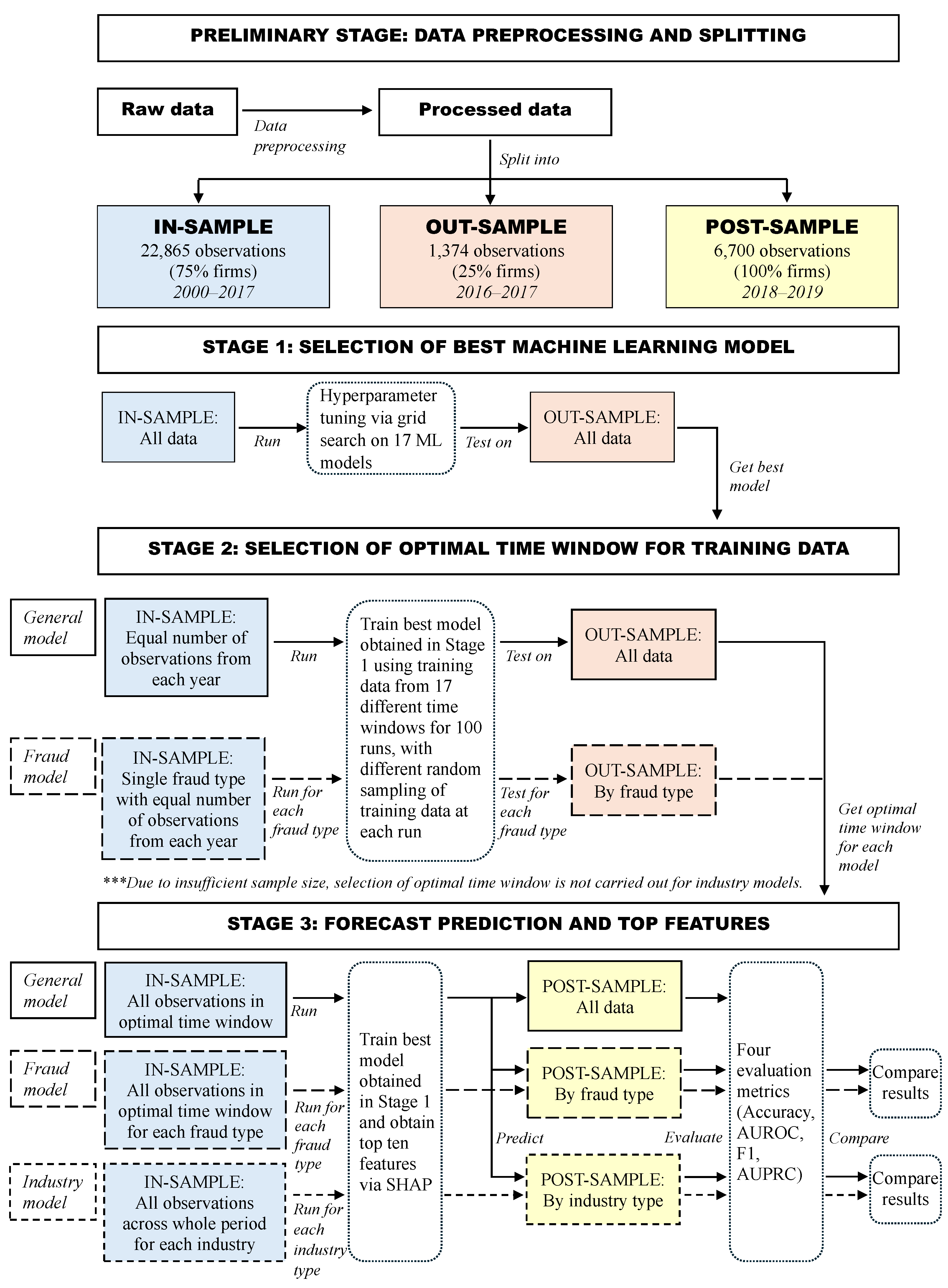
Complementing the above literature, we propose a comprehensive framework for Chinese corporate fraud prediction which incorporates the unaddressed or rarely addressed aspects in the literature. We first collected observations for all fraud types from 2000 to 2020 and extract yearly corporate governance information and financial indices from firm’s annual reports as features. These data were combined as firm-year observations to form the full dataset. To accommodate for segmented models, the full dataset was broken down into data by fraud type and data by industry. The experiments were divided into three stages, each serving a different purpose. In the first stage, we carried out the selection of best machine learning model with the full data. Five machine learning classifiers were selected and combined with three resampling techniques that handle the class imbalance problem to form 15 classifier–resampling combinations. We further employed two ensemble-based resampling approaches to make up a total of 17 candidate models. We found that the random forest classifier without resampling performed best among the 17 models according to the average ranking of four performance measures.
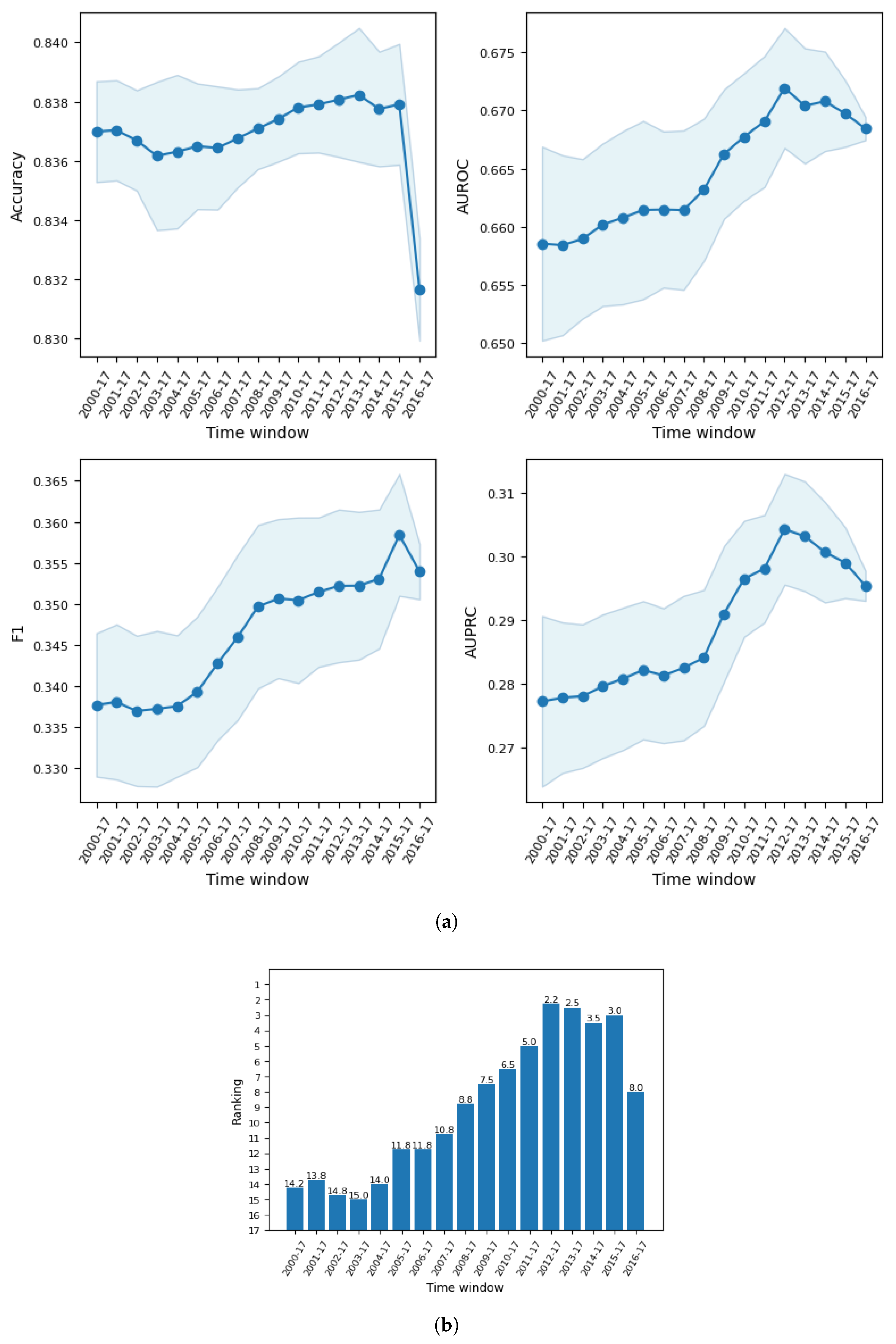
The second stage involved dealing with population drift, where selection of optimal time window for training data was carried out for the general model based on the full data and the fraud segmented models based on the data by fraud type. Our results indicate that the predictive performance increased gradually as older data were discarded from the training sample until at some time period when the number of training examples became too small and performance began to decline. In particular, when predicting fraud occurrences in 2016 to 2017, the general model reported the best performance when training data prior to 2012 were discarded. For the same test window, all the optimal time windows found in the fraud segmented models excluded training data before 2010. This suggests that population drift exists in our data, and it may be caused by several reasons such as changing corporate behavior, socio-economic conditions, and regulatory policy. This manifests the need to balance the tradeoff between the most recent data and sufficient data in order to obtain the best model performance.
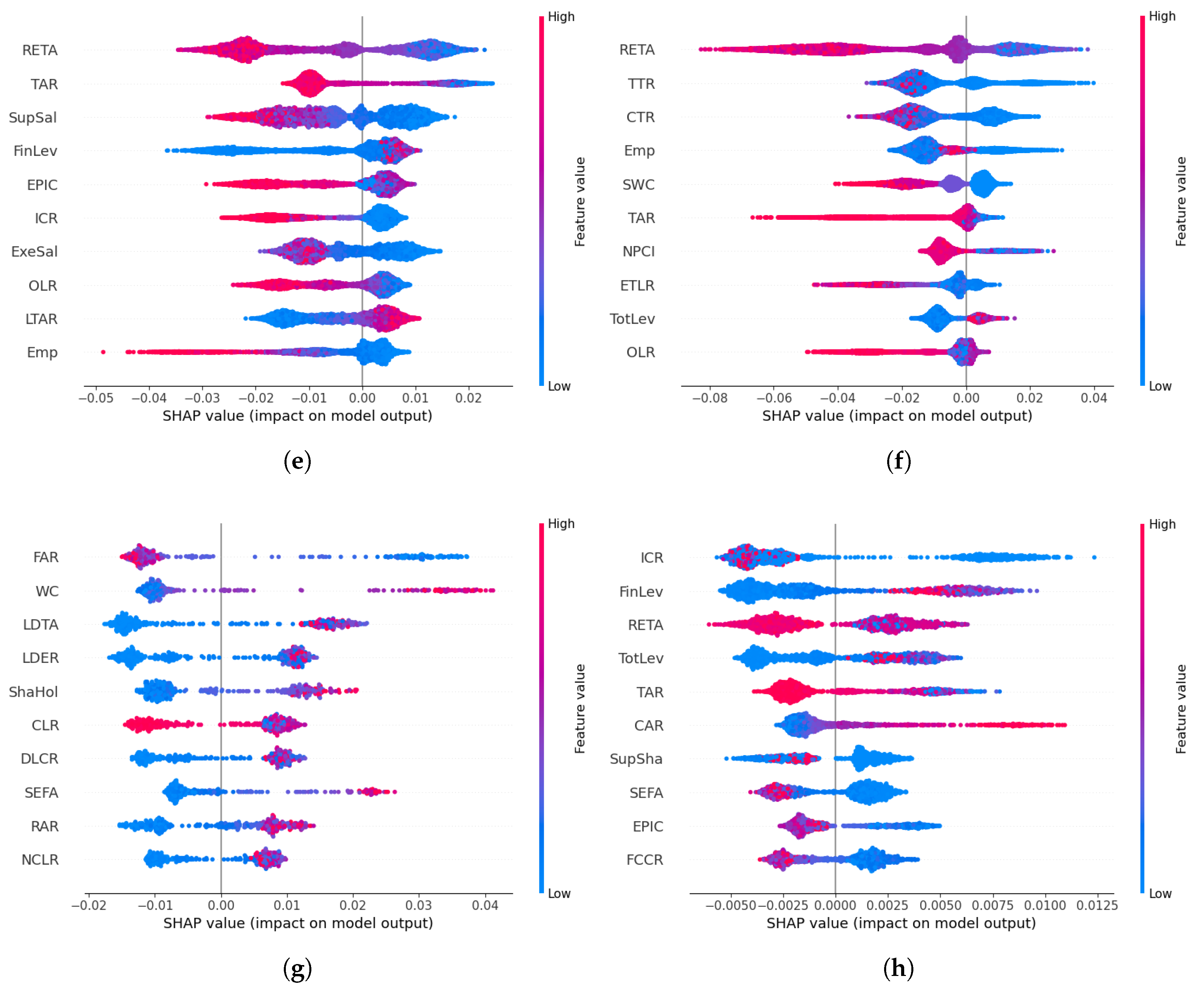
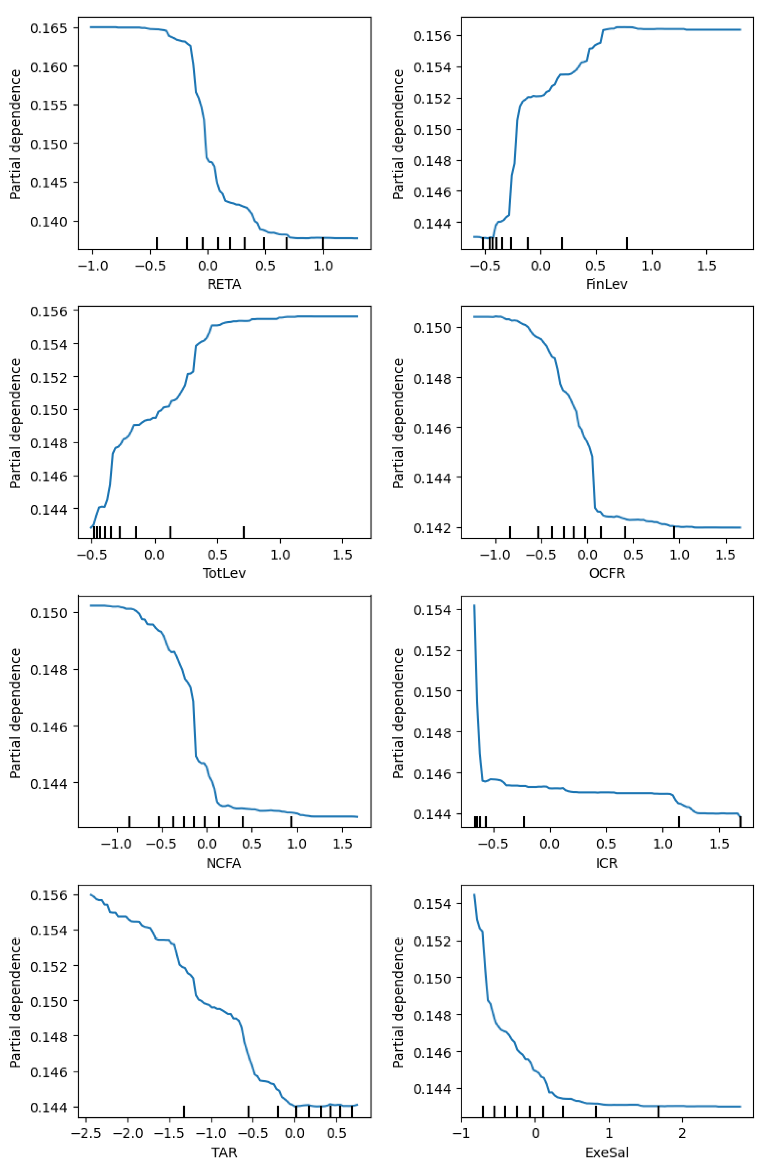
Thirdly, using the best model and optimal time window, we built a general model and segmented models for fraud types and industries. The forecast performance results of the general model, evaluated by four metrics, are comparable to the model performance reported in the previous literature. In terms of feature importance, the risk level and solvency features emerged as top features in the general model. Next, we compared the general model with each segmented model according to predictive performance and top features associated with fraud occurrence. Our findings revealed that five out of nine segmented models for fraud type achieved a better performance than their respective predictions using the general model. Among these fraud types, four of them have low fraud rates (<2%), and two of them show a significant discrepancy in terms of top features. On the other hand, only 2 out of 12 segmented models for industry performed better than their respective predictions in the general model. Our further investigation indicates that this is due to the insufficient training sample for most of the industries. In particular, we found that when we controlled the training size, the segmented models were as good as, or even better than the general model in terms of the AUROC for 11 of the 12 industries. These results suggest that segmented models are more informative than the general model for fraud types with low fraud rates and most industries given sufficient training data and that they should be employed to investigate fraud occurrence for important fraud types and industries.
This paper contributes to the literature on Chinese corporate fraud detection in the following ways. Firstly, to the best of our knowledge, our study is the first paper to address the population drift problem in corporate fraud prediction. This is a common yet important subject in credit scoring, and methods have been proposed to handle this in multiple credit scoring scenarios [12,13,14]. However, none of the previous research considered population drift when building models to predict corporate fraud. We fill this gap by incorporating the selection of an optimal time window for training data before the main model is built. Our results shed new light on the impact of handling population drift in corporate fraud detection.
Secondly, our research provides new insights on the use of segmented models in corporate fraud prediction by introducing new dimensions for segmentation according to fraud type and industry. This is rarely seen in the literature, as previous studies focus on model for specific fraud types and large industries. Fraud predictions for less prevalent fraud types and small industries are understudied. We built segmented models for nine fraud types and 12 industries with sufficiently large sample sizes. The segmented models allow us to (1) compare the predictive performances between general model and segmented model; (2) understand which fraud types/industries are more difficult to predict; and (3) investigate the main risk features associated with each fraud/industry. This offers a new perspective on corporate fraud prediction to researchers, practitioners, and regulators.
Thirdly, our paper complements the growing literature on Chinese corporate fraud detection by providing a comprehensive framework to predict corporate fraud. In particular, we include all observations and fraud types in our model. The features employed in our model can be easily extracted from readily available annual reports and directly used without sophisticated feature engineering approaches. We have also proposed a clear three-stage experimental design that takes into account data splitting, machine learning algorithms, evaluation metrics, and methods to handle the class imbalance and population drift problems which are common in fraud prediction problem. Furthermore, we introduce segmented models for fraud type and industry to carry out comparisons between general and segmented models based on predictive performance and top features. We argue that we have taken into account most if not all aspects of corporate fraud prediction in our framework. Our work may serve as a practical reference for future research.
The remainder of the paper is organized as follows: We start with a review of the existing research on corporate fraud detection in Section 2. In Section 3, we discuss the data used in our study and how the data are split to carry out the experiments, as well as the methodology implemented in our experiments, which includes methods to handle the population drift problem, segmented models, and experimental design, which is divided into three stages. The results for each stage are reported in Section 4, with discussion and analysis to draw meaningful insights. Concluding remarks are provided in Section 5.

2. Related Studies

There is ample research on implementing machine learning for corporate fraud prediction in the literature. We focus on some of the most frequently cited research findings in the past 15 years. Most of these studies carry out fraud prediction based on data obtained from US companies. Cecchini et al. [15] proposed a financial kernel for support vector machine which managed to identify 80% of management frauds using basic financial data. Perols [16] compared the performances of six machine learning models in detecting financial statement frauds under different assumptions of fraud-to-non-fraud ratios. Surprisingly, they found that logistic regression and support vector machine outperformed artificial neural network and ensemble models.
Kim et al. [17] developed multiclass classifiers to carry out financial misstatement predictions which classified the violations into intentional, unintentional, and no violation instead of the usual binary classification approach. Hájek and Henriques [18] proposed a fraud detection system which incorporates automatic feature selection of financial and linguistic data. Their findings show that random forest and Bayesian belief network performed best in terms of true positive rate and true negative rate, respectively. Perols et al. [19] introduced observation undersampling to address class imbalance and variable undersampling by fraud type, which improved the model prediction results by approximately 10% compared to the best-performing benchmark model. Brown et al. [20] utilized a topic modeling algorithm to predict financial misreporting and found that thematic content of financial statement improved fraud prediction by up to 59%.
Bao et al. [21] compared fraud prediction performance using different combinations of classifiers and input variables. Their findings indicate that the combination of RUSBoost and raw financial data outperformed the other combinations across four evaluation metrics. Bertomeu et al. [22] carried out misstatement predictions and found that gradient-boosting regression tree and RUSBoost performed best on likelihood-based and classification-based measure performance, respectively. Khan et al. [23] proposed a fraud detection framework based on minimizing the loss function and maximizing the recall that was optimized using a meta-heuristic algorithm called Beetle Antennae Search (BAS), which outperformed several benchmark models across different evaluation metrics. Also using the optimization approach, Yi et al. [24] incorporated the Egret Swarm Optimization Algorithm (ESOA) into their fraud detection framework. The proposed model outperformed several benchmark models, including BAS, over four performance measures.
Since we utilized Chinese data in our research, we also report some recent studies related to corporate fraud prediction in Chinese firms in Table 1. We present several important aspects of this research in the table for a clear and concise comparison. These include the time period of the data, fraud type of interest, number of observations, fraud rate, and categories of features employed. The feature categories will be further discussed in Section 3.1. We also report the number of machine learning algorithms and evaluation metrics used, as well as four binary indicators on whether the class imbalance problem, population drift problem, segmented models, or feature importance was implemented in these studies.
Ravisankar et al. [25] compared the performance of six machine learning models for detecting financial statement fraud with and without feature selection. They found that a probabilistic neural network model outperformed the remaining models in both cases. Song et al. [26] proposed a hybrid framework which combines machine learning models and a rule-based system for financial statement fraud detection. Using the ensemble of four classifiers, their results indicate that non-financial risk factors and rule-based system reduce the error rates of predictions. Liu et al. [27] documented that random forest performed best in the detection of financial frauds, and the ratio of debt to equity was the most important variable in the model. Yao et al. [28] compared the combination six machine learning models with the dimensionality reduction method and found that the combination of support vector machine and stepwise regression dimension reduction performed best in financial statement fraud detection.
Achakzai and Juan [8] built a voting classifier and stacked classifier for financial statement fraud predictions and found that these meta-classifiers performed better than standalone classifiers in detecting fraudulent observations. Wu and Du [29] implemented deep learning models on the combination of numerical and textual data to detect financial statement frauds. Their results indicate that LSTM and GRU with textual data showed considerable improvement in model performance compared to traditional models with numerical data. Xu et al. [10] compared six machine learning models and studied the effects of different features categorized by greed, opportunity, need, exposure (GONE) on corporate fraud prediction. Their findings revealed that random forest performed best and suggest that exposure variables are more important than other variables. Chen and Zhai [30] utilized data from China to compare the performance of five ensemble learning models on financial statement fraud detection and found that bagging outperformed boosting in several evaluation indicators. Lu et al. [11] documented that XGBoost performed best among five models in corporate fraud prediction, and their results indicate that financial condition has the greatest impact in fraud detection among different feature groups. Rahman and Zhu [31] investigated accounting fraud detection in Chinese family firms and found that imbalanced ensemble classifiers performed better than conventional classifiers.
Cai and Xie [32] proposed an explainable financial statement fraud detection approach based on a two-layer knowledge graph (FSFD-TLKG). They compared the proposed method with 17 different explainable and non-explainable models and found that it outperformed all models except the non-explainable XGBoost model. Duan et al. [9] used ensemble learning to investigate financial statement frauds with the proposal of an ex ante fraud risk index which improves the integrity of the financial information. Li et al. [6] utilized textual data from company’s financial statements and media’s news reports to represent internal and external perceptions, respectively. They found that using multiperspective enhanced the effectiveness of financial fraud detection. Sun et al. [33] documented that the XGBoost model outperformed traditional models in identifying financial frauds among Chinese companies. Tang and Liu [7] proposed a transformer-based architecture which implements feature extraction and handles class imbalance problem using the multiattention algorithm to carry out financial fraud detection. The proposed method outperformed traditional models across five performance metrics.
Based on the literature review, we observe three aspects which are rarely addressed or are completely unaddressed in the existing studies. Firstly, to the best of our knowledge, none of the research related to corporate fraud in China addresses the population drift problem in their studies. Population drift occurs due to the change in distribution over time, and it is a common problem in credit scoring. Over the years, approaches have been proposed to handle this problem in different credit scoring scenarios such as mortgage arrear prediction [12], bad rate among accepts (BRAA) prediction [13,35], consumer behavioral scoring [14], and credit card fraud detection [36]. Since we employed data that span multiple years to carry out corporate fraud detection, we believe that the population drift problem is present and should be addressed in our experiments.
Secondly, we observe that the uses of segmented models are mainly for subsets of different features [28,29,34] or time periods [8,31,33] in existing studies regarding Chinese corporate fraud. Since the data consist of firms from different industries, we hypothesize that a segmented model can be utilized to investigate fraud occurrence in each industry. This is rarely seen in the literature, as existing studies focus on specific industries which are large [6,7].
Thirdly, most of the extant research focuses on a single fraud type, with financial statement fraud being the most commonly investigated fraud type. Even though there are more than ten fraud types in the data, only a few studies considered all of them [10,11]. We hypothesize that all fraud types should receive equal attention regardless of their prevalence. This can be achieved by building a general model which takes into account all types of violation and extending the idea of a segmented model to each fraud type, which is unseen in the literature so far.

3. Materials and Methods

3.1. Data

The data employed in our experiments were taken from the China Stock Market and Accounting Research (CSMAR) database [37]. The following information was retrieved from the CSMAR website:
  • Company profile such as company name, industry, and establishment date.
  • Annual corporate governance information for each company.
  • Annual or quarterly financial indices for each company.
  • Information on detection of frauds based on China Securities Regulatory Commission (CSRC) enforcement actions.
The initial sample consisted of data spanning from 2000 to 2020. CSMAR records the fraud revelation year and fraud occurrence year for 14 different fraud types and firms from 19 different industries. Following Lu et al. [11], we dropped two fraud types which were deemed as less severe, namely, delayed disclosure and false information disclosure. We also dropped firms from the finance industry. This is a common practice in the literature due to the significant differences in the definition of financial statements and accounting methods for financial firms [30]. The target variable F r a u d for year t is constructed for each firm based on fraud occurrence year, which takes the value of 1 if a firm commits any of the 12 frauds in year t and 0 otherwise. Multiple frauds committed by a firm in the same year are treated as a single observation so that there is only one observation for each firm-year.
To carry out fraud prediction, we matched frauds from year t with corporate governance and financial information from year t 1 . For quarterly financial report, the average value was taken to represent the financial indices for a particular year. With this, we were left with data from 2000 to 2019, where data in year 2000 represent corporate governance and financial information from 2000, fraud occurrence in 2001, and so forth. After all the calculations and merging, we obtained a total of 37,125 firm-year observations.
The observations were split based on the train–validation–test approach. Since our data consist of firm-year observations across a number of firms spanning over 20 years, they are considered as panel data. We utilized the method proposed by Granger and Huang [38] to split the data. In particular, the data were split into the in-sample, out-sample, and post-sample based on their respective firm and year. This arrangement simulates the real deployment of a fraud detection system. The in-sample and out-sample selections were the training and test set for model development, and the post-sample selection simulated the operational use of model post-development.
The in-sample set contains 75% of the firm-year observations from 2000 to 2017. This served as the training sample to carry out model building. The remaining 25% of the firm-year observations went into the out-sample set. We split the data in a way that the firms in in-sample and out-sample did not intersect, i.e., a firm’s observations were either entirely in in-sample or entirely in out-sample. The out-sample served as the validation sample, which was used for model selection. However, we only kept data from 2016 to 2017 in the out-sample set, and we discarded the remaining data. By doing so, we obtained a validation sample which had (1) the closest possible time period and trend to the post-sample; (2) a comparable violation rate as the post-sample; and (3) the same time duration (2 years) as the post-sample. These characteristics would allow us to select an optimal model for forecast prediction. Finally, the post-sample contained all firm-year observations from 2018 to 2019 and served as the test sample for our experiment.
Table 2 presents the number of observations, fraud count, and fraud rate for each sample. The in-sample contains 22,865 firm-year observations, and 2808 (12.28%) of the observations involve fraud. The out-sample consists of 1374 observations with 223 (16.23%) fraud occurrences. The post-sample contains 6700 observations, where 1166 (17.40%) of them are fraudulent observations. We observe that the fraud rates in recent years are higher, and this necessitates a validation set which contains recent data to ensure the model selected is more precise. The breakdown of number of observations and fraud rate by year are presented in Table A1 in Appendix A.
Data preprocessing was carried out after data split. To minimize information leakage, the preprocessing tasks were carried out based on in-sample, that is, we applied the model built based on in-sample on all three sample sets. We first applied winsorization at top and bottom 1% and standardization on numerical features to remove outliers. Categorical features were one-hot encoded into binary features. We adopted a standard approach to handle missing values, where the mean (or mode) was imputed for numerical (or nominal) features [39]. We further included indicator variables to represent whether a feature was missing. The processed data produced 241 features. Feature selection and feature engineering can be usefully applied for corporate fraud detection [10,32]. In our study, we followed Chen and Zhai [30] by using all original features in the model build. The reason for this is that machine learning models tend to internalize feature selection, transformation, and interaction effects through built-in algorithms like LASSO penalty in logistic regression, feature number in tree-based models, and non-linear transformation in kernel-based models and neural networks. Hence, all available features are retained to preserve the original effects of the features. These features were categorized into four groups according to the file it was drawn from in the CSMAR database, namely, corporate governance, profitability, risk level, and solvency. The features which belonged to neither of these categories were grouped into the fifth category as others. Table 3 provides a brief description for each category and presents the number of features in each category.

3.2. Dealing with Population Drift

A vital issue in credit scoring is to model the likelihood of the population to evolve and change with time [5]. This scenario is commonly known as population drift and often occurs as a result of economic pressures and changing environment. Population drift can be classified into abrupt and gradual drifts based on its rate of change, where the former represents a sudden change in distribution at a certain time point, while the latter represents a steady change over time [40]. As mentioned in Section 3.1, the violation rate is higher in recent years than older years, and this suggests population drift in our data. This may indicate an abrupt shift due to the change in regulation policy [4], a gradual shift as a result of economic recession [26], or even a combination of both. A common approach to deal with the problem is to carry out re-estimation of the classifier’s parameters at different intervals based on a recent subset of data [35]. However, this is difficult and time-consuming, since the occurrence of population drift is unpredictable. Nevertheless, the population drift problem needs to be addressed, as it may cause a deterioration in classification performance. In our experiment, we dealt with population drift using the selection of optimal time window for training data.

Selection of Optimal Time Window for Training Data

To address the population drift problem, we have to minimize the impact of irrelevant data in our model. Trends change as time evolves, and this causes older data to become less relevant. Therefore, they should be excluded in model building to ensure that the model is able to learn the correct trend. This brings us to the next task, which is the identification of an optimal time point such that all data before the time point are removed. According to Qian et al. [41], this can be done by selecting the optimal time window for the training set. The optimal time window is defined as the time period which contains the subset of training data that gives the best model performance in the validation set among different time periods. Once the optimal time window is determined, the subset of training data within the time window is kept for subsequent models, whereas all the remaining training data outside the time period are discarded.

3.3. Segmented Models

Segmentation in credit scoring is the process of identifying homogeneous populations with respect to their predictive relationships [42]. Our data consist of firms from different industries committing different types of fraud over a span of 20 years. It is hence interesting to study whether the fraud patterns are different for each fraud type and industry and to what extent do they differ from the general trend. To achieve this, we considered segmented models for some of the fraud types and industries which have sufficiently large samples. This allowed us to (1) compare the predictive performances between general model and segmented model; (2) understand which fraud type and industry are more difficult to predict; and (3) investigate the main risk features associated with each fraud type and industry.

3.3.1. Segmented Model for Fraud Type

There are 12 fraud types in our sample. For each of the fraud type i, we define the target variable F r a u d i , t which assigns the value of 1 if a firm commits fraud i in year t and 0 otherwise. For example, if a firm commits fraud P2501 but not fraud P2502 in year 2010, we will have F r a u d P 2501 , 2010 = 1 , whereas F r a u d P 2502 , 2010 = 0 for the firm. Since fraud is committed, the target variable F r a u d for the particular firm-year observation takes the value of one in the general model.
The number of fraud count and fraud rate for each of the fraud type in all three samples are presented in Table A2 in Appendix A. We used the same data split for the segmented models so that the number of observations in each sample would be consistent across the general model and segmented models. However, the fraud count for each fraud type did not sum to the fraud count in Table 2, as some firms committed multiple frauds in the same year.
We observed that false record and material omission were the two dominant fraud types over the years, and some fraud types had extremely low fraud rates. In particular, there were three fraud types which recorded no fraud observation in both the out-sample and post-sample, namely, fraudulent listing, insider trading, and stock price manipulation. Since we would not be able to carry out validation and testing, segmented models were not built for these fraud types. Finally, we were left with nine segmented models for fraud type.

3.3.2. Segmented Model for Industry

According to the 2012 CSRC industry code, firms in China are classified into 19 different industries and assigned letters A to S to represent their respective industry. The breakdown of observations and fraud rate by industry in in-sample and post-sample for each industry are presented in Table A3 in Appendix A. Firms from the finance industry (Industry J) were dropped, whereas firms from the service industry (Industry O) are not present in the data, making a total of 17 industries in our data. The breakdown for out-sample is not reported because it was not employed in segmented models for industry. This is further discussed in Section 3.4.
We observe that more than half of the observations are from the manufacturing industry, whereas the agriculture industry and the healthcare industry have the highest fraud rates among all industries. Since some industries have few observations, segmented models were only built for industries with more than 300 observations in in-sample. As a result, we only built segmented models for 12 industries, dropping accommodation and catering (Industry H), research and technology (Industry M), education (Industry P), healthcare (Industry Q), and others (Industry S).

3.4. Experimental Setup

After data splitting and preprocessing, the setup of the experiment was divided into three stages. The first stage involved the selection of machine learning model; the second stage focused on the selection of optimal time window for training data; and the third stage involved forecast prediction and identification of top features based on the selections in the first two stages. Figure 1 presents a flow chart as a brief overview of the experiments and data involved at each stage.

3.4.1. Stage 1: Selection of Best Machine Learning Model

The primary target of the first stage is to select the best machine learning model for the subsequent stages. Based on the literature, we selected five machine learning classifiers as candidates. This included logistic regression, which is widely regarded as the typical model for credit scoring and support vector machine and has been proven to be effective in the literature [15,16]. We also employed two ensemble classifiers, namely, random forest and gradient boosting, which have been found to outperform traditional models in several studies [10,22,30]. In particular, for gradient boosting, we employed the XGBoost variant, since several recent studies documented that it performed best in corporate fraud detection [11,32,33]. Finally, we employed an artificial neural network model with two hidden layers, since it has been shown in the literature that, generally, deep learning models do not perform well for credit scoring task [39]. As fraud prediction involves unbalanced data, apart from the original data without resampling, we employed Synthetic Minority Oversampling Technique (SMOTE) [43] and cost-sensitive learning to deal with the class imbalance problem. In particular, cost-sensitive learning is achieved by including an extra hyperparameter c l a s s _ w e i g h t in model building in Python 3.11. We followed the combinatorial approach presented in Yang et al. [44] by combining the machine learning classifiers and resampling techniques to obtain 15 (5 × 3) classifier–resampling combinations. Since the use of ensemble-based resampling approaches is also popular [8,9,34], we further employed two ensemble approaches, namely, the RUSBoost classifier and the balanced random forest classifier, in our experiments. Since resampling is integrated in these classifiers, they are considered as individual models and were not combined with resampling techniques. These classifiers were combined with the 15 classifier–resampling combinations to make up a total of 17 machine learning candidate models.
For each of the 17 candidate model, we carried out hyperparameter tuning via grid search to select the best hyperparameter set based on the average AUROC across five-fold cross-validation on in-sample data. With the best hyperparameter set, the models were trained using the entire in-sample data and tested on out-sample data. This was repeated three times with different random states to ensure the stability and robustness of the models. Most extant research in the literature has utilized a few performance measures to assess the model performance. Lessmann et al. [45] also mention that it is beneficial to consider multiple metrics to obtain a comprehensive performance evaluation. We employed four metrics, namely, accuracy, area under receiving operating characteristics curve (AUROC), F1-score, and area under precision–recall curve (AUPRC), to evaluate the model performance. As a method to handle class imbalance, we implemented threshold optimization via Youden index (J) [46] to determine the optimal threshold for accuracy and F1 based on the in-sample. The Youden index is a measure that determines the effectiveness of the ROC curve, which can be computed by taking the difference between the true positive rate (sensitivity) and false positive rate (1—specificity). The optimal threshold of a model can be determined by selecting the cutoff point with the highest Youden index. To determine the best machine learning model, we adopted the average rank ( A v g R ) approach proposed by Lessmann et al. [45]. The model performance was ranked across all models for each evaluation metric, and the average value of the four rankings was computed. The model with the highest average ranking was selected as the best model and employed in subsequent stages.

3.4.2. Stage 2: Selection of Optimal Time Window for Training Data

The main goal of the second stage is to select the optimal time window for training data. For this task, we started with the whole in-sample data which contained firm-year observations from 2000 to 2017. At each run, we carried out stratified sampling and randomly selected an equal number of observations from each year to make up a training sample of 5000 observations. This was done to ensure that data from all years were equally represented in the training sample. A model (which was the best machine learning model obtained in Stage 1) was trained on the selected data and tested on the out-sample data. After that, data from the oldest year were discarded and replaced by an equal number of observations from each of the remaining years such that the size of the training sample remained unchanged at 5000 observations. The substitute data were drawn via stratified sampling from the unused training data pool. A new model was then trained on the updated sample and tested on the same out-sample data. The ‘data update’ step was repeated to obtain training samples for all 17 time windows, for which the training sample of the last time window contained 2500 observations each from 2016 and 2017.
To compensate for the randomness arising from data sampling, the process was repeated for 100 iterations. In other words, there were 100 training samples, trained models, and out-sample outcomes for each of the 17 time windows. Similar to the previous stage, the outcomes were assessed based on four evaluation metrics, and the average values of the metrics over 100 runs were calculated. These values were separately ranked across all time windows, and the time window with the highest average ranking across four metrics was selected as the optimal time window for training data.
The selection of optimal time window was also implemented for segmented models for fraud types. The same process which included data sampling and data update for 17 time windows was repeated for 100 iterations to select the optimal time window for each of the nine fraud segmented models, with the only difference being the data employed. Instead of the full in-sample data, we used in-sample data by fraud type, as mentioned in Section 3.3, to carry out data sampling. Similarly, the trained models were tested and evaluated on out-sample data by fraud type. On the other hand, we did not implement selection of optimal time window in segmented models for industry type due to limited sample size, with the exception of the manufacturing industry, where the same process mentioned above was conducted to select the optimal time window using observations whose firms were from the manufacturing industry.

3.4.3. Stage 3: Forecast Prediction and Top Features

In the third stage, we carried out forecast prediction and determine the top features for the general model and each segmented model. Based on the experiments in the first two stages, we trained the general model and each segmented model for fraud using all available observations within the optimal time window determined in Stage 2. This was also carried out in segmented model for the manufacturing industry. For the other industry segmented models, all the observations in in-sample which belonged to the industry were used for model training. The trained models were then used to carry out forecast prediction on the post-sample data. In particular, the post-sample data were separated into three categories, i.e., full data, data by fraud type, and data by industry. We used the general model to predict the occurrence of fraud on all three categories, whereas the segmented models were applied to their respective groups. For the general model and each segmented model, we extracted the top ten features associated with model predictions and grouped them into categories based on Table 3. Based on the extant literature, we implemented SHAP (Shapley additive explanations) to determine the top features for each model. This allows us to conduct global interpretations on feature importance and their interactions with the target variable. Comparisons were carried out between the general model and segmented models based on two aspects—prediction outcome evaluated using four metrics and top features associated with each fraud and industry.

4. Results and Discussion

4.1. Best Machine Learning Model

In this section, we report the best machine learning model based on the model performances on the out-sample data evaluated using four metrics. All 17 candidate models were trained on the full in-sample data based on the best hyperparameter set determined using grid search. The best hyperparameter set with its respective candidate values for each model is presented in Table A4 in Appendix A. Figure 2 provides a visual representation of the performances of each machine learning model, as reported in Table A5 in Appendix A. In particular, Figure 2a illustrates the accuracy, AUROC, F1, and AUPRC of the models when tested on out-sample data. As mentioned in Section 3.4, all the models were trained for three runs to ensure their stability and robustness. The values for each run are presented in bars, while the lines represent their means across three runs. These means were separately ranked across all models for each metric, and the average rankings across four metrics are presented in Figure 2b.
Based on the results, we found that random forest outperformed other classifiers without oversampling, whereas gradient boosting performed best when cost-sensitive learning and SMOTE were applied, but the latter is negligible, since it is the worst of the three resampling methods. Logistic regression had a moderate performance, as it ranked middle among the classifiers for all three resampling methods. Support vector machine, on the other hand, performed well with cost-sensitive learning but not quite well with no oversampling and SMOTE. The artificial neural networks, despite showing decent performance in some runs, were not as stable as the other models, as portrayed by the fluctuations across multiple runs. In terms of resampling methods, all classifiers performed best with cost-sensitive learning, with logistic regression and random forest being the exceptions. On the other hand, SMOTE did not show good performances, as it ranked in the bottom among the resampling methods for all machine learning classifiers. For ensemble-based resampling approaches, RUSBoost and balanced random forest both produced decent performances, as their average rankings are ranked among the top five across 17 candidate models.
We observed that the random forest–non-oversampling combination had the best performance across four evaluation metrics on out-sample data with an average ranking of 2.8. This agrees with the findings of Xu et al. [10], whose results indicate that random forest outperformed five machine learning models in Chinese corporate fraud detection. It is also similar to the results reported in Chen and Zhai [30], where they found that the bagging model outperformed several boosting models in a few evaluation metrics. Henceforth, the combination of random forest and non-oversampling was employed in subsequent stages unless stated otherwise.

4.2. Optimal Time Window for Training Data

Selection of the optimal time window for training data was carried out for the general model, for all segmented models for fraud types, and for the segmented model for the manufacturing industry. Figure 3 presents the out-sample performances for the models trained using data from different time windows, as reported in Table A6 in Appendix A. Figure 3a depicts the mean accuracy, AUROC, F1, and AUPRC, with the shaded region representing the standard deviation over 100 runs for each time window, whereas Figure 3b presents the average ranking across four metrics over 100 runs for each time window where the selection of the optimal time window was based on.
According to the results, 2012 to 2017 was selected as the optimal time window for the general model, as it achieved the best average ranking of 2.2 across four metrics. We employed all data within the time window to train the model in the subsequent stage. We observed that there was a gradual improvement in model performances when older data were excluded, until reaching the maximum point at 2012, after which further removal of data led to a decline in performance. This may be due to the lack of volume of data. While this indicates that dealing with the population drift problem results in an improvement in model performance, it also suggests that there is a tradeoff between most recent data and sufficient data in order to obtain the optimal performance. Therefore, searching for the optimal time point to discard data is indeed an important step when dealing with population drift.
The optimal time window for each segmented model for fraud type and the manufacturing industry are tabulated in Table 4. Based on the results, we found that five segmented models for fraud type achieved the best performance when the optimal time window of training data was either two or three years, while the remaining four fraud types performed best when prior data up to six to eight years were included in training. An interesting point to observe is that only two of the optimal time windows for the fraud segmented models matched the optimal time window for the general model. Although this is slightly counterintuitive, it is sensible, since the general model is not a direct combination of segmented models for fraud, as multiple fraud occurrences within the same year are taken as a single occurrence in the former.
On the other hand, the optimal time window for the manufacturing industry model agrees with the general model. Since the manufacturing industry accounts for more than half of the observations in the general model, it is natural that the fraud patterns in the industry dominates the general model. These results indicate that the optimal time point to discard data may vary for different tasks and may even differ when predicting over a different time period. This suggests that corporate fraud models should be updated from time to time, and segmented models can be employed for the investigation of specific cases. Despite being different, none of the optimal time windows includes data prior to 2010. This manifests the need to handle the population drift problem and suggests that when the sample size is large enough, we should attempt to carry out drift analysis to ensure that irrelevant observations are excluded in model building for segmented models.

4.3. Forecast Prediction Results

In this section, we report the post-sample prediction results for general model and segmented models. We employed the random forest classifier to train the models based on all in-sample data in the optimal time window, as reported in Table 4. These models were trained without oversampling, with the exception of the fraud segmented models for fictitious asset (P2502), unauthorized change in capital usage (P2509), and illegal stock trading (P2512), in which cost-sensitive learning was applied with the ‘ c l a s s _ w e i g h t ’ parameter set as ‘ b a l a n c e d ’, since the class distribution is extremely unbalanced (less than 1 % positive events). For industry segmented models other than the manufacturing industry, all available data in in-sample were utilized to build the models. In terms of training time, all models recorded a training time of less than a minute, with the general model recording a training time of 38 s. Apart from training size, we observed that the fraud rate also affected the training time of the model.
The general model reported an accuracy of 0.8127, an AUROC of 0.7452, an F1-score of 0.4433, and an AUPRC of 0.3864 on the post-sample data, which are comparable to the performances reported in Xu et al. [10] and Lu et al. [11] on a different but overlapped test period. Figure 4 illustrates the post-sample prediction results for each fraud type of the general model and its respective segmented model, which were evaluated using four metrics. The corresponding plots for the industry segmented models are presented in Figure 5. The values for these plots are given in Table A7 in Appendix A. We have also included the prediction results of the general model on the entire post-sample data in the plots for industry segmented models. This can be seen as the average across the performance of the general model on the post-sample data for each industry, since the post-sample data by industry were obtained via breaking up the entire post-sample data according to its industry, and the fraud rate of the entire post-sample data was calculated as the average of the fraud rates of each post-sample data by industry. On the other hand, we could not directly compare the predictive performance of the general model on post-sample data by fraud type with its predictive performance on the entire post-sample data. This is because the post-sample data by fraud type are not the direct segmentation of the entire post-sample data, and the significant differences in fraud rates between the data have resulted in deviations in the F1-scores and AUPRC scores. Therefore, comparisons can only be made on a within-fraud-segment basis between the predictive performance of general model (trained using entire in-sample data) and each segmented model (trained using in-sample data by fraud type) on the post-sample data of the particular fraud type. The models with better performance among the four metrics between the general model and segmented models for each fraud type and each industry are tabulated in Table 5 and Table 6, respectively.
We found that five out of nine segmented models for fraud type achieved a better performance than their respective prediction results using the general model. They are fictitious profit, fictitious asset, unauthorized change in capital usage, occupancy of company’s asset, and illegal stock trading. We further observed that these fraud types all had low fraud rates, where four of them had the lowest post-sample fraud rate among the nine fraud types. The low F1-scores and AUPRC scores for these fraud types are likely due to the extremely unbalanced class distribution, since F1 and AUPRC both integrate precision and recall, and these metrics can be greatly affected by class imbalance. However, this is not an unusual observation, as Xu et al. [10] also reported a low F1-score in a segmented model for more serious frauds, which included two of the aforementioned fraud types (fictitious profit and fictitious asset). Nevertheless, the segmented models demonstrated an improvement compared to the general model. This is sensible, because when all frauds are included in a model (as in the case of the general model), it will lean toward the more prevalent fraud type. The results suggest that segmented models should be utilized to carry out predictions for frauds which are important but less common. On the other hand, there were four fraud types whose segmented models’ predictive performances did not outperform that of the general model. This indicates that their fraud patterns are better captured by the general model and suggests that the information from other frauds may be transferable to these frauds.
In terms of the segmented models for industry, only 2 out of 12 segmented models (agriculture and real estate) for industry achieved a better performance than their respective prediction results using the general model. The results indicate that the performance outcomes of the segmented models are not as good as the general model for most industries. We speculate that this is because the training size is small in each segment and hence insufficient to build an informative segmented model. To verify our hypothesis, we plotted a learning curve of model performance (AUROC) against training set size for each of the ten industries whose segmented models were outperformed by the general model. The results show that when we control the training set size, the segmented models have a comparable if not better predictive performance, i.e., showing higher learning curves, than their respective performance outcomes of the general model for nine of the ten industries, with the wholesale and retail industry being the only exceptional case. This provides justification to our conjecture and suggests that the superior predictive performance of the general model compared to the segmented models for industry is due to the information gained as a result of transfer learning from the additional training samples in other industries. Nevertheless, when the sample size is large enough, we should attempt to build segmented models for industries, as they are more informative than the general model in most cases. As illustration, we present two of the learning curve plots in Figure 6, namely, the manufacturing industry and power, gas, and water industry. The former has the largest sample size, whereas the latter demonstrates the largest difference in the AUROC between the general and segmented models when the training size is controlled. The post-sample AUROC for the general model and segmented model for industry when the training size is fixed to be the sample size of each respective industry is presented in Table A8 in the Appendix A.
Since the general model can be considered as an average across all industries, we further compared the performance of the general model on each industry. If the data from an industry have a better performance than most of the segmented models for other industries and the overall model, this indicates that fraud occurrences in the particular industry can be more easily predicted than other industries. Hence, we observed that fraud occurrences in the power, gas, and water; construction; leasing and commercial; and culture and sports industries were easier to predict, whereas fraud occurrences in the agriculture, information technology, and real estate industries were harder to predict compared to other industries. An interesting point to observe is that the industries which are harder to predict are exactly the industries for which the general model’s performance did not outperform their respective segmented models’ performances. The observation suggests that the information from other industries is not transferrable to these industries, and hence, the use of segmented model is indispensable.

4.4. Top Features for Each Model

In this section, we report the top ten features for the general model and each segmented model obtained using SHAP 0.46.0. Table 7 presents the category distribution of these features based on categories described in Table 3. We further computed the sum of the absolute difference between the number of features in the general model and each segmented model over all categories. Although the features may be different despite being in the same category, we argue that features of the same category exhibit similar aspects of a company, and hence, the absolute difference can be seen as a straightforward dissimilarity measure for the top features. We observed that for fraud segmented models, the segmented model for fictitious asset (P2502) had the greatest dissimilarities when compared to the general model, in which its top features were dominated by corporate governance information. The top features for unauthorized change in captial usage (P2509), on the other hand, were mainly solvency features. The segmented models for fictitious profit (P2501), material omission (P2505), and illegal guarantee (P2514) had the same category distribution with the general model, whereas the top features for the remaining fraud types were distributed across all four categories. For industry segmented models, the segmented model for power, gas, and water industry (Industry D) had the greatest dissimilarities with the general model among the industry segmented models, whereas the top features for agriculture industry (Industry A) were mainly solvency features. An interesting point to observe is that none of the segmented models for industry had the same category distribution as the general model, with construction industry (Industry E) and culture and sports industry (Industry R) being the only industry pairs which shared the same category distribution. This indicates that each industry has its unique top features and further manifests the need to build segmented models for a better comprehension of these industries.
We took a step further to investigate the top features for the general model and segmented models for fraud types and industries which had better predictive performances than the general model. Figure 7 presents the SHAP summary plots of the top ten features for the general model and seven segmented models, as reported in Table A9 in Appendix A. To further enhance model interpretability, we plotted the partial dependence plots for the features in general model which also appeared as top features in segmented models, as shown in Figure 8. We observed that risk level features played an important role in Chinese corporate fraud detection with three of the top four features in the general model from this category. In particular, the retained earnings to total assets (RE/TA) ratio emerged as the top feature, showing a negative association with the occurrence of fraud. We observed that its risk effect flattened at extreme values of the RE/TA ratio, and this indicates that outliers do not have a distorting effect in the model. This was followed by financial leverage in the second and total leverage in the fourth, both showing a positive association with fraud, with risk effects flattening at extreme high values. This finding agrees with Xu et al. [10], where the leverage ratio had the highest feature importance after the exposure variables, which were not included in our model. A similar finding was also reported in Duan et al. [9], where the leverage ratio ranked fourth based on feature importance.
Solvency features also demonstrated significant impacts on corporate fraud prediction, with five of the top ten features coming from this category. This includes earnings before interest; the taxes, depreciation, and amortization (EBITDA) to total liabilities ratio, operating cash flow ratio (OCFR); net cash flow from operating activities (NCFA); the interest coverage ratio (ICR); and the tangible assets ratio, all of which yielded a negative association with the target variable fraud. In particular, both OCFR and NCFA produced a similar relationship with fraud as the RE/TA ratio. This agrees with findings in the existing literature, as several studies have reported net cash flow from operating activities as one of the top ten features with greatest importance [11,30,34]. The ICR, on the other hand, showed a drastic change in risk effect on low values, and the risk effect flattened out as its value increased. In terms of corporate governance information, we found that executive’s salary and management’s salary produced a negative association with the likelihood of fraud, where the former showed an exponentially decreasing relationship with fraud. Finally, none of the profitability features appeared as top features in the general model.
Next, we compared the top features between the general model and segmented models by fraud type. There were five segmented models whose predictive performances were better than their respective performance results of the general model. We started with the models whose category distribution differed most from the general model. The category distribution of the top features for fictitious asset (P2502) showed a huge discrepancy with the general model, where none of the top features overlapped with the general model. We observed that corporate governance information played a vital role in the detection of fictitious asset, and on the contrary, none of the top features belonged to the risk level category. The top features for unauthorized change in capital usage (P2509) also showed a great disparity with the general model, with solvency features dominating the top features. There were only two overlapping features when compared to the general model, namely, net cash flow from operating activities and operating cash flow ratio. These features were negatively associated with the target variable, as in the case of the general model. However, they had a larger effect on fraud compared to the general model, as suggested by the feature importance.
We observed that profitability features had a significant impact in the detection of illegal stock trading (P2512), and the role of solvency features was less important compared to the general model. Three of the top ten features overlapped with the top features in the general model, including the RE/TA ratio, which appeared as the top feature in both lists. They all showed the same direction of association with the target variable as the general model but had a much higher feature importance compared to the general model. The category distribution of the top features for occupancy of company’s asset (P2510) was similar to the general model, with five overlapping features between the models and RE/TA ratio as the top feature in both models. All the overlapping features had the same direction of association with the target variable as the general model. Similar to other segmented models, these features also had a larger impact on fraud than the general model. Finally, nine of the top ten features for fictitious profit (P2501) were different from the general model, despite having the same feature distribution as the general model. The only overlapping feature between the models was the RE/TA ratio, which emerged as the top feature, was negatively associated with the target variable, and had a larger effect compared to the general model.
As for the industry segmented models, only two segmented models outperformed the general model in forecast prediction. The top features for the agriculture industry (Industry A) showed some disparity with the general model, with eight of the top ten features coming from the solvency category. At the feature level, none of these features overlapped with the general model. This observation provides support on the dominant performance of the segmented model over the general model despite having a small sample size. On the other hand, the top five features for the real estate industry (Industry K) appeared in the top features for the general model. Nevertheless, we observed non-linear relationships between financial leverage, RE/TA ratio, and total leverage and the target variable, which differed from the relationships portrayed in the general model. The discrepancies in the direction of association caused the general model to perform badly on this industry and be outperformed by the segmented model.
The RE/TA ratio emerged as the top feature in the general model and multiple segmented models, indicating its prominent effect in Chinese corporate fraud detection. In fact, it is one of the four financial indicators used to derive the Altman’s Z China score, which identifies potential distress in Chinese firms [47]. A higher RE/TA ratio indicates that a company’s operations are mainly funded by its internal resources rather than external debt or capital. It reflects the financial strategy and growth ability of a firm and is positively correlated with a company’s financial health. In general, the existing literature reports a negative relationship between the RE/TA ratio and the occurrence of fraud [48,49], suggesting that a financially unhealthy firm is more likely to be involved in corporate fraud.

5. Conclusions

We conducted Chinese corporate fraud prediction by incorporating the selection of an optimal time window to address the population drift problem and segmented models for fraud types and industries. This was achieved via a three-stage experimental design that served different purposes at each stage. The first stage involved the selection of the best machine learning model from 17 candidate models. Random forest without oversampling emerged as the model with the best predictive performance across four evaluation metrics. We then carried out the selection of an optimal time window for the training data for the general model and segmented models for fraud types. We found that when testing on data in 2016 to 2017, the optimal time window for all models excluded training data prior to 2010. The results indicate that population drift exists in fraud detection, and addressing it leads to an improvement in predictive performance.
Using the best model and optimal time window found, we built a general model and segmented models for nine fraud types and 12 industries. Our findings indicate that five segmented models for fraud type achieved better performance than their respective predictions using the general model, out of which four of them had low fraud rates. In terms of industry segmented models, even though only two segmented models outperformed the respective performances of the general model, our investigation reveals that this is due to insufficient training set size for most of the models. In particular, we found that 11 segmented models for industries had comparable or even better performance in terms of the AUROC when we controlled the training size. Also, we have identified dissimilarities between the top features of the general model and segmented models for fraud types and industries whose predictive performance results were better in segmented models. These findings suggest that segmented models should be employed to investigate fraud occurrence for important fraud types and industries given sufficient training samples.
In summary, the main findings of this study are the following:
  • Random forest classifier without resampling emerged as the best machine learning model for Chinese corporate fraud prediction.
  • Population drift exists in corporate fraud prediction, and addressing it using different time windows for training data selection led to an improved predictive performance.
  • The optimal time windows for the general model and segmented models for fraud type suggest the use of historical data within three to eight years for model building to diminish the effect of population drift.
  • Segmented models have a better predictive performance than the general model for fraud types with low fraud rates and are as good as the general model for most industries when controlling for training set size.
  • Risk level and solvency features emerged as the top features associated with corporate fraud for the general model and segmented models for most fraud types and industries.
Our study provides practical information for different parties and contributes to the existing literature on Chinese corporate fraud detection. Firstly, we shed new light on the impact of population drift in corporate fraud detection, which is unaddressed in the current literature despite being applied in different credit scoring scenarios. It enhances the understanding of academic researchers and practitioners regarding the importance of addressing the population drift problem. Secondly, we provide new insights on the use of segmented models in corporate fraud prediction by improving the understanding of differences between the various fraud types and industries in terms of the risk features associated with each segment and how relatively easier or more difficult it is to predict fraud within each segment. These results offer a new perspective on corporate fraud prediction for regulators and policymakers. Thirdly, we propose a comprehensive framework to predict corporate fraud in China. Apart from Chinese firms, the general framework and methodologies can also be implemented on firms in other regions like the US and EU, since class imbalance and population drift are common problems in corporate fraud prediction internationally. The only difference is that there may be other perspectives which are uniquely available in these markets for segmentation that would need to be taken into account in the analysis. In general, our study provides a practical framework for future research in the domain.
This study has several limitations. Firstly, due to a limited sample size, the segmented models for most industries are not as informative as the general model. Future research could focus on enhancing the predictive performance given a limited sample size by developing a better framework for information extraction or including additional information such as textual data in the model. Techniques in transfer learning can also be utilized to extract transferable information from the general model. Secondly, the unbalanced class distribution resulted in low F1-scores and AUPRC scores due to high false positives. In order to boost the F1-scores and AUPRC scores, improving the precision and recall rate, especially in the case of extremely unbalanced class distribution, is also an important task in the future research. This could possibly be achieved by considering alternative machine learning algorithms or resampling techniques. Furthermore, the main focus of this study is on Chinese corporate fraud prediction, and we did not consider data from other regions in our study. Since the general framework is applicable to firms in other regions, future work could consider applying this experimental design framework to historical fraud data in other jurisdictions.

Author Contributions

Conceptualization: C.C.G. and A.B.; Methodology: C.C.G., Y.Y. and A.B.; Formal analysis: C.C.G.; Data curation: C.C.G.; Writing—original draft: C.C.G.; Writing—review and editing: Y.Y., A.B. and X.H.; Supervision: A.B. and X.H.; Funding acquisition: A.B. and X.H. All authors have read and agreed to the published version of the manuscript.

Funding

We are grateful to Ningbo Municipal Government for funding of this project as part of grant number 2021B-008-C. We are also grateful to Ningbo Science and Technology Bureau for Key Plan Program for funding the project as a part of grant numbers 2022Z243 and 2022Z173.

Institutional Review Board Statement

Not applicable.

Informed Consent Statement

Not applicable.

Data Availability Statement

The data were obtained from the China Stock Market and Accounting Research Database (CSMAR) and are publicly available at https://data.csmar.com/, accessed on 7 March 2023.

Acknowledgments

We would like to thank the anonymous reviewers for providing suggestions on the methodologies used in the experiments.

Conflicts of Interest

The authors declare that they have no known competing financial interest or personal relationships that could have appeared to influence the work reported in this paper.

Appendix A. Additional Tables

Table A1. Number of observations and violation rate by year in in-sample, out-sample, and post-sample.
YearNo. of ObservationsViolation CountViolation Rate
In-sample
2000605548.93%
20017399512.86%
20027858210.45%
2003824688.25%
2004889788.77%
2005954646.71%
2006934717.60%
20071002848.38%
200811051099.86%
2009111813011.63%
2010119813311.10%
2011150320613.71%
2012167123113.82%
2013175022913.09%
2014178021111.85%
2015185625913.95%
2016195131316.04%
2017220139117.76%
Total22,865280812.28%
Out-sample
201664710215.77%
201772712116.64%
Total137422316.23%
Post-sample
2018332861318.42%
2019337255316.40%
Total6700116617.40%
Table A2. Fraud count and fraud rate for each fraud type.
Fraud TypeIn-SampleOut-SamplePost-Sample
CountRateCountRateCountRate
P2501 Fictitious profit3451.51%402.91%1301.94%
P2502 Fictitious asset770.34%90.66%330.49%
P2503 False record16027.01%1299.39%78311.69%
P2505 Material omission18127.92%14510.55%69810.42%
P2507 Fraudulent listing130.06%00.00%00.00%
P2509 Unauthorized change in capital usage1490.65%282.04%771.15%
P2510 Occupancy of company’s asset4091.79%483.49%3194.76%
P2511 Insider trading30.01%00.00%00.00%
P2512 Illegal stock trading820.36%20.15%460.69%
P2513 Stock price manipulation20.01%00.00%00.00%
P2514 Illegal guarantee3281.43%463.35%2333.48%
P2515 Mishandling of general account6662.91%443.20%2163.22%
Table A3. Number of observations and fraud rate for each industry.
IndustryIn-SamplePost-Sample
Obs. (%)Fraud (%)Obs. (%)Fraud (%)
A—Agriculture356 (1.56%)88 (24.72%)77 (1.15%)13 (16.88%)
B—Mining710 (3.11%)91 (12.82%)141 (2.10%)26 (18.44%)
C—Manufacturing12,960 (56.68%)1563 (12.06%)4295 (64.09%)731 (17.02%)
D—Power, gas, and water1054 (4.61%)111 (10.53%)217 (3.24%)26 (11.98%)
E—Construction607 (2.65%)100 (16.47%)187 (2.79%)31 (16.58%)
F—Wholesale and retail1451 (6.35%)173 (11.92%)319 (4.76%)63 (19.75%)
G—Transport and storage839 (3.67%)62 (7.39%)197 (2.94%)19 (9.64%)
H—Accommodation and food94 (0.41%)6 (6.38%)13 (0.19%)1 (7.69%)
I—Information technology1584 (6.93%)247 (15.59%)534 (7.97%)118 (21.97%)
K—Real estate1477 (6.46%)147 (9.95%)229 (3.42%)35 (15.28%)
L—Leasing and commercial473 (2.07%)60 (12.68%)117 (1.75%)35 (29.91%)
M—Research and technology125 (0.55%)6 (4.80%)83 (1.24%)11 (13.25%)
N—Environment335 (1.47%)34 (10.15%)110 (1.64%)17 (15.45%)
P—Education86 (0.38%)12 (13.95%)19 (0.28%)6 (31.58%)
Q—Healthcare105 (0.46%)23 (21.90%)24 (0.36%)5 (20.83%)
R—Culture and sports420 (1.84%)56 (13.33%)111 (1.66%)23 (20.72%)
S—Others189 (0.83%)29 (15.34%)27 (0.40%)6 (22.22%)
Total22,865 (100%)2808 (12.28%)6700 (100%)1166 (17.40%)
Table A4. Best hyperparameter set and its respective candidate values for each machine learning model.
ModelHyperparameterCandidate ValuesBest Value
LR-NOC0.0001, 0.001, 0.01, 0.1, 10.01
LR-CSLC0.0001, 0.001, 0.01, 0.1, 10.01
class_weight1:1, 1:2, 1:3, 1:4, balancedbalanced
LR-SMOTEC0.0001, 0.001, 0.01, 0.1, 1, 2, 3, 5, 8, 105
SVM-NOkernellinear, polynomial, rbfrbf
C0.5, 1, 1.5, 2, 3, 52
gamma1/1000, 1/500, 1/200, 1/100, 1/50, 1/20, 1/101/50
SVM-CSLkernellinear, polynomial, rbfrbf
C0.5, 1, 1.5, 2, 3, 4, 53
gamma1/5000, 1/4000, 1/3000, 1/2000, 1/1000, 1/5001/3000
class_weight1:1, 1:2, 1:3, 1:4, balancedbalanced
SVM-SMOTEkernellinear, polynomial, rbfrbf
C1, 2, 3, 4, 5, 6, 8, 10, 128
gamma1/1000, 1/500, 1/200, 1/100, 1/50, 1/20, 1/101/20
RF-NOn_estimators500, 1000, 20001000
max_depth10, 15, 20, 25, 30, 4025
max_features10, 15, 2015
RF-CSLn_estimators500, 1000, 20001000
max_depth10, 15, 20, 25, 3020
max_features10, 15, 2015
class_weight1:1, 1:2, 1:3, 1:4, balancedbalanced
RF-SMOTEn_estimators500, 1000, 2000, 30002000
max_depth10, 15, 20, 25, 3020
max_features10, 20, 30, 40, 50, 60, 80, 10080
GB-NOgamma0, 5, 105
max_depth3, 5, 8, 10, 155
subsample0.5, 0.6, 0.7, 0.8, 10.6
learning rate0.01, 0.05, 0.10.05
GB-CSLgamma0, 5, 10, 1510
max_depth3, 5, 8, 10, 155
subsample0.5, 0.6, 0.7, 0.8, 10.5
learning rate0.01, 0.05, 0.10.05
class_weight1:1, 1:2, 1:3, 1:4, balanced1:2
GB-SMOTEgamma0, 5, 100
max_depth5, 10, 15, 20, 25, 30, 4030
subsample0.5, 0.6, 0.8, 10.6
learning rate0.01, 0.05, 0.1, 0.20.1
ANN-NObatch size64, 128 256, 512256
no. of epochs10, 20, 30, 50, 10010
no. of neurons10, 20, 30, 50, 10020
ANN-CSLbatch size64, 128, 256, 512256
no. of epochs10, 20, 30, 50, 10010
no. of neurons10, 20, 30, 50, 10010
class_weight1:1, 1:2, 1:3, 1:4, balancedbalanced
ANN-SMOTEbatch size32, 64, 128 256, 51264
no. of epochs20, 50, 100, 150, 200150
no. of neurons20, 50, 100, 200, 300, 400, 500400
RUSBoostn_estimators20, 50, 100, 200, 50050
learning rate0.5, 0.6, 0.7, 0.8, 10.5
BRFn_estimators500, 1000, 2000, 3000, 4000, 50003000
max_depth5, 10, 15, 2010
max_features10, 15, 20, 25, 3020
Table A5. Out-sample accuracy, AUROC, adjusted F1, and AUPRC for each machine learning model. Numbers 1st, 2nd, and 3rd refer to the results of three separate runs, and R indicates to the rank of the mean value across 17 models.
ModelAccuracyAUROCF1AUPRCAvg.
1st2nd3rdMeanR1st2nd3rdMeanR1st2nd3rdMeanR1st2nd3rdMeanR Rank
Non-oversampling
LR-NO0.87710.87710.87710.877140.65170.65170.65170.651790.27540.27540.27540.275490.20500.20500.20500.205087.5
SVC-NO0.78160.78160.78160.7816170.58030.58020.58020.5802150.23220.23220.23220.2322120.16660.16660.16660.16661514.8
RF-NO0.87720.87700.87710.877140.66440.66410.66410.664230.28430.28410.28350.284020.21430.21480.21440.214522.8
GB-NO0.85450.85130.85510.8536140.65980.66710.66040.662540.27950.27760.28260.279950.20890.21170.21300.211246.8
NN-NO0.87210.87180.87430.8727130.63220.66250.65400.6495100.26390.28430.27560.2746100.19010.20750.20140.19971111.0
Cost-sensitive learning
LR-CSL0.87540.87540.87540.8754100.65380.65380.65380.653880.27820.27820.27820.278270.20440.20440.20440.204498.5
SVC-CSL0.87750.87750.87750.877510.65380.65380.65380.653870.27820.27820.27820.278280.20580.20580.20580.205875.8
RF-CSL0.87590.87470.87300.8745110.66520.66580.66420.665110.28610.28850.28690.287210.21240.21210.21040.211634.0
GB-CSL0.87670.87630.87660.876580.66010.66570.66710.664320.27630.28080.28900.282030.21270.21330.21890.215013.5
NN-CSL0.87680.87700.87720.877060.64420.65410.65020.6495110.27010.27390.26560.2699110.19640.20850.19990.2016109.5
SMOTE
LR-SMOTE0.87500.87360.87140.8733120.63150.63270.63180.6320130.04450.05910.06360.0557150.19020.19090.19000.19041213.0
SVC-SMOTE0.87720.87720.87720.877220.57730.57640.57630.5767160.02140.02380.02560.0236170.15640.15560.15530.15581713.0
RF-SMOTE0.83510.84180.83700.8380160.61910.62160.62300.6212140.14660.14330.15270.1475140.17470.17670.17790.17651414.5
GB-SMOTE0.87620.87590.87540.875890.64390.64970.63810.6439120.03680.03260.03670.0354160.19320.19060.18710.19031312.5
NN-SMOTE0.84730.84280.84030.8435150.55100.57620.57630.5678170.14320.15960.15880.1539130.15170.16250.16670.16031615.3
Ensemble-based resampling approaches
RUSBoost0.87720.87720.87720.877220.64870.65810.65860.655160.27580.27780.28250.278760.20180.21200.20600.206665.0
BRF0.87640.87660.87670.876670.65780.65770.65850.658050.28280.28010.27790.280340.20920.20930.20970.209455.3
Bold font indicates the best performance and the highest ranking across 17 models for each metric. For non-oversampling and cost-sensitive learning models, the only difference between each run is the random state of each model; hence, both LR and SVM have the same results across all three runs.
Table A6. Mean and standard deviation for accuracy, AUROC, AUPRC, and F1 over 100 runs for general model trained using each time window. R indicates the rank of the mean values across 17 time windows.
TimeAccuracyAUROCF1AUPRCAvg.
WindowMean (SD)RMean (SD)RMean (SD)RMean (SD)RRank
2000–20170.8370 (0.0017)100.6585 (0.0084)160.3377 (0.0087)140.2772 (0.0134)1714.3
2001–20170.8370 (0.0017)90.6584 (0.0078)170.3381 (0.0094)130.2778 (0.0119)1613.8
2002–20170.8367 (0.0017)120.6589 (0.0069)150.3370 (0.0092)170.2781 (0.0113)1514.8
2003–20170.8362 (0.0025)160.6602 (0.0070)140.3372 (0.0095)160.2796 (0.0113)1415.0
2004–20170.8363 (0.0026)150.6608 (0.0075)130.3376 (0.0086)150.2808 (0.0112)1314.0
2005–20170.8365 (0.0021)130.6614 (0.0077)110.3393 (0.0092)120.2821 (0.0109)1111.8
2006–20170.8364 (0.0021)140.6615 (0.0067)100.3427 (0.0093)110.2813 (0.0106)1211.8
2007–20170.8368 (0.0017)110.6614 (0.0069)120.3459 (0.0101)100.2825 (0.0114)1010.8
2008–20170.8371 (0.0014)80.6632 (0.0061)90.3497 (0.0100)90.2841 (0.0107)98.8
2009–20170.8374 (0.0014)70.6663 (0.0056)80.3506 (0.0097)70.2910 (0.0107)87.5
2010–20170.8378 (0.0015)50.6677 (0.0055)70.3504 (0.0101)80.2966 (0.0091)66.5
2011–20170.8379 (0.0016)40.6691 (0.0056)50.3514 (0.0091)60.2981 (0.0085)55.0
2012–20170.8381 (0.0019)20.6720 (0.0052)10.3522 (0.0093)50.3044 (0.0087)12.2
2013–20170.8382 (0.0023)10.6704 (0.0050)30.3522 (0.0090)40.3032 (0.0087)22.5
2014–20170.8378 (0.0019)60.6708 (0.0043)20.3530 (0.0085)30.3007 (0.0079)33.5
2015–20170.8379 (0.0020)30.6697 (0.0029)40.3584 (0.0074)10.2991 (0.0056)43.0
2016–20170.8317 (0.0017)170.6685 (0.0010)60.3539 (0.0034)20.2954 (0.0024)78.0
Bold font indicates the best performance and the highest ranking across 17 time windows for each metric.
Table A7. Forecast prediction results on post-sample data. GM and SM each stands for general model and segmented model, respectively.
ModelFraudAccuracyAUROCF1AUPRCBest
RateGMSMGMSMGMSMGMSM
General (Entire post-sample data)17.40%0.8127-0.7452-0.4433-0.3864--
Segmented models for fraud type
P2501 Fictitious profit1.94%0.96670.95110.77590.81100.08440.16870.07740.0791SM
P2502 Fictitious asset0.49%0.97790.99480.76870.81560.02160.10260.02010.0920SM
P2503 False record11.69%0.88240.88320.75580.75200.35840.35020.30480.2966GM
P2505 Material omission10.42%0.89150.89590.73150.73200.31010.30830.25000.2446Tie
P2509 Unauthorized change in capital usage1.15%0.97050.97760.67390.74360.04410.10000.01920.0660SM
P2510 Occupancy of company’s asset4.76%0.93970.92910.75010.75590.17210.20320.11610.1394SM
P2512 Illegal stock trading0.69%0.97630.99310.66680.66680.02240.09410.05360.0958SM
P2514 Illegal guarantee3.48%0.95400.95090.77970.76170.13860.18140.13210.1330Tie
P2515 Mishandling of general account3.22%0.95390.93880.76470.73360.13540.14190.09420.0857GM
Segmented models for industry
A—Agriculture16.88%0.83120.77920.67430.76560.31750.43480.38510.4058SM
B—Mining18.44%0.82980.81560.75280.70470.47300.34380.47300.3412GM
C—Manufacturing17.02%0.83170.83260.74770.74030.43960.42470.38520.3748GM
D—Power, gas, and water11.98%0.88020.88020.77730.77100.44160.33850.47480.2875GM
E—Construction16.58%0.82890.83420.77460.69310.41030.31030.38820.3432GM
F—Wholesale and retail19.75%0.79310.80250.75440.70320.41940.39880.39880.3851GM
G—Transport and storage9.64%0.90360.90360.74510.73920.35000.31250.30340.1972GM
I—Information technology21.97%0.78650.79590.71290.69190.47790.43410.42370.4523Tie
K—Real estate15.28%0.84720.84720.67280.74700.32260.31250.28480.3166SM
L—Leasing and commercial29.91%0.71790.65810.78850.66200.62370.53450.57790.4471GM
N—Environment15.45%0.86360.84550.75840.72420.37840.27270.44370.3014GM
R—Culture and sports20.72%0.79280.79280.78260.69020.53850.38890.47220.3663GM
Bold font indicates the best performance between general model and segmented model for each metric.
Table A8. Post-sample AUROC for the general model and segmented models for industry when training size was fixed to be the sample size of each respective industry.
IndustryPost-Sample AUROC
GMSM
A—Agriculture0.59510.7615
B—Mining0.67510.7032
C—Manufacturing0.74030.7412
D—Power, gas, and water0.62410.7744
E—Construction0.59000.6989
F—Wholesale and retail0.72430.7022
G—Transport and catering0.64240.7469
I—Information technology0.68680.6916
K—Real estate0.62010.7425
L—Leasing and commercial0.64800.6541
N—Environment0.61990.7324
R—Culture and sports0.64420.6901
Bold font indicates the best performance between general model and segmented model.
Table A9. Top 10 features for general model and selected segmented models based on SHAP. RF R. indicates the ranking of each feature based on feature importance of random forest model.
RankFeature nameAbbr.Cat.Imp.EffectRF R.
(a) General model
1Retained earnings to total assets ratioRETAR0.0085Negative1
2Financial leverageFinLevR0.0040Positive3
3EBITDA to total liabilities ratioETLRS0.0037Negative4
4Total leverageTotLevR0.0031Positive8
5Operating cash flow ratioOCFRS0.0030Negative12
6Net cash flow from operating activitiesNCFAS0.0028Negative16
7Interest coverage ratioICRS0.0028Negative13
8Tangible assets ratioTARS0.0027Negative7
9Executive’s salaryExeSalC0.0027Negative5
10Management’s salaryMgmSalC0.0025Negative9
(b) P2501—Fictitious profit
1Retained earnings to total assets ratioRETAR0.0161Negative1
2Shareholders’ equity to fixed assets ratioSEFAR0.0095Positive9
3Conformity rate for long-term assetsCRLAS0.0092Positive5
4Fixed assets ratioFARS0.0091Negative4
5Executives’ sharesExeShaC0.0086Positive8
6Cash ratioCRS0.0085Non-linear15
7Operating leverageOpeLevR0.0084Negative10
8No. of employeesEmpC0.0079Negative7
9Non-current assets ratioNCAS0.0078Non-linear2
10Liabilities to equity market cap ratioLEMCS0.0075Non-linear6
(c) P2502—Fictitious asset
1No. of supervisors without compensationSWCC0.0203Negative1
2Managers’ sharesMgrShaC0.0177Positive2
3Supervisor’s salarySupSalC0.0135Negative3
4Chairman’s sharesChaShaC0.0126Positive4
5Executives’ sharesExeShaC0.0123Positive6
6Management’s sharesMgmShaC0.0119Positive5
7Liabilities to tangible assets ratioLTARS0.0113Positive9
8Directors’ salaryDirSalC0.0110Negative7
9Directors’ sharesDirShaC0.0109Positive10
10Fixed assets ratioFARS0.0097Negative8
(d) P2509—Unauthorized change in capital usage
1Financial liabilities ratioFLRS0.0299Positive1
2Operating liabilities ratioOLRS0.0289Negative2
3Conformity rate for long-term assetsCRLAS0.0171Positive3
4Quick ratioQRS0.0121Positive5
5Net cash flow from operating activitiesNCFAS0.0110Negative4
6Shareholders’ equity to fixed assets ratioSEFAR0.0095Positive7
7Cash assets ratioCARS0.0091Positive14
8Fixed assets ratioFARS0.0088Negative6
9Operating cash flow ratioOCFRS0.0078Negative8
10Composite tax rateCTRP0.0075Negative9
(e) P2510—Occupancy of company’s asset
1Retained earnings to total assets ratioRETAR0.0149Negative1
2Tangible assets ratioTARS0.0107Negative4
3Supervisor’s salarySupSalC0.0100Negative2
4Financial leverageFinLevR0.0095Positive3
5Equity attributable to parent company to invested capital ratioEPICP0.0084Non-linear7
6Interest coverage ratioICRS0.0080Negative10
7Executives’ salaryExeSalC0.0078Negative11
8Operating liabilities ratioOLRS0.0074Negative8
9Liabilities to tangible assets ratioLTARS0.0074Positive12
10No. of employeesEmpC0.0065Negative6
(f) P2512—Illegal stock trading
1Retained earnings to total assets ratioRETAR0.0255Negative1
2Turnover tax rateTTRP0.0138Negative2
3Composite tax rateCTRP0.0136Negative3
4No. of employeesEmpC0.0116Non-linear6
5No. of supervisors without compensationSWCC0.0099Negative10
6Tangible assets ratioTARS0.0095Negative4
7Net profit to comprehensive income ratioNPCIP0.0080Negative14
8EBITDA to total liabilities ratioETLRS0.0079Negative5
9Total leverageTotLevR0.0078Positive16
10Operating liabilities ratioOLRS0.0076Non-linear7
(g) Industry A—Agriculture
1Fixed assets ratioFARS0.0159Negative1
2Working capitalWCS0.0144Positive2
3Long-term debt to total assets ratioLDTAS0.0141Positive3
4Long-term debt to equity ratioLDERS0.0110Positive5
5No. of shareholdersShaHolC0.0102Positive6
6Current liabilities ratioCLRS0.0092Non-linear7
7Debt to long-term capital ratioDLCRS0.0090Positive8
8Shareholders’ equity to fixed assets ratioSEFAR0.0085Positive4
9Receivable assets ratioRARS0.0081Positive9
10Non-current liabilities ratioNCLRS0.0075Positive10
(h) Industry K—Real estate
1Interest coverage ratioICRS0.0047Negative1
2Financial leverageFinLevR0.0038Non-linear2
3Retained earnings to total assets ratioRETAR0.0029Non-linear3
4Total leverageTotLevR0.0028Non-linear5
5Tangible assets ratioTARS0.0027Negative6
6Cash assets ratioCARS0.0022Positive4
7Supervisors’ sharesSupShaC0.002Non-linear22
8Shareholders’ equity to fixed assets ratioSEFAR0.002Negative14
9Equity attributable to parent company to invested capital ratioEPICP0.0019Negative17
10Fixed charged coverage ratioFCCRS0.0019Negative10
Bold feature name in segmented models indicates the feature also appears as a top 10 feature in general model.

References

  1. Wells, J.T. Corporate Fraud Handbook: Prevention and Detection, 5th ed.; John Wiley & Sons, Inc.: Hoboken, NJ, USA, 2017. [Google Scholar]
  2. Warren, J. Occupational Fraud 2024: A Report to the Nations; Technical Report; Association of Certified Fraud Examiners (ACFE): Austin, TX, USA, 2024; Available online: https://legacy.acfe.com/report-to-the-nations/2024 (accessed on 5 March 2025).
  3. Cressey, D.R. Other People’s Money; A Study in the Social Psychology of Embezzlement; Patterson Smith: Montclair, NJ, USA, 1953. [Google Scholar]
  4. Zuo, Y.; Liu, X.; Jiang, F.; Shen, S. Sharpened “Real Teeth” of China’s securities regulatory agency: Evidence from CEO turnover. Int. Rev. Econ. Financ. 2024, 96, 103637. [Google Scholar] [CrossRef]
  5. Hand, D.J.; Henley, W.E. Statistical Classification Methods in Consumer Credit Scoring: A Review. J. R. Stat. Society. Ser. A (Stat. Soc.) 1997, 160, 523–541. [Google Scholar] [CrossRef]
  6. Li, G.; Wang, S.; Feng, Y. Making differences work: Financial fraud detection based on multi-subject perceptions. Emerg. Mark. Rev. 2024, 60, 101134. [Google Scholar] [CrossRef]
  7. Tang, Y.; Liu, Z. A Distributed Knowledge Distillation Framework for Financial Fraud Detection Based on Transformer. IEEE Access 2024, 12, 62899–62911. [Google Scholar] [CrossRef]
  8. Achakzai, M.; Juan, P. Using Machine learning Meta-Classifiers to detect financial frauds. Financ. Res. Lett. 2022, 48, 102915. [Google Scholar] [CrossRef]
  9. Duan, W.; Hu, N.; Xue, F. The information content of financial statement fraud risk: An ensemble learning approach. Decis. Support Syst. 2024, 182, 114231. [Google Scholar] [CrossRef]
  10. Xu, X.; Xiong, F.; An, Z. Using Machine Learning to Predict Corporate Fraud: Evidence Based on the GONE Framework. J. Bus. Ethics 2022, 186, 137–158. [Google Scholar] [CrossRef]
  11. Lu, Q.; Fu, C.; Nan, K.; Fang, Y.; Xu, J.; Liu, J.; Bellotti, A.G.; Lee, B.G. Chinese corporate fraud risk assessment with machine learning. Intell. Syst. Appl. 2023, 20, 200294. [Google Scholar] [CrossRef]
  12. Whittaker, J.; Whitehead, C.; Somers, M. A dynamic scorecard for monitoring baseline performance with application to tracking a mortgage portfolio. J. Oper. Res. Soc. 2007, 58, 911–921. [Google Scholar] [CrossRef]
  13. Adams, N.M.; Tasoulis, D.K.; Anagnostopoulos, C.; Hand, D.J. Temporally-Adaptive Linear Classification for Handling Population Drift in Credit Scoring. In Proceedings of the International Conference on Computational Statistics, Paris, France, 22–27 August 2010; pp. 167–176. [Google Scholar]
  14. Nikolaidis, D.; Doumpos, M.; Zopounidis, C. Exploring population drift on consumer credit behavioral scoring. In Proceedings of the Operational Research in Business and Economics: 4th International Symposium and 26th National Conference on Operational Research, Chania, Greece, 4–6 June 2015; Springer: Cham, Switzerland, 2017; pp. 145–165. [Google Scholar]
  15. Cecchini, M.; Aytug, H.; Koehler, G.; Pathak, P. Detecting Management Fraud in Public Companies. Manag. Sci. 2010, 56, 1146–1160. [Google Scholar] [CrossRef]
  16. Perols, J. Financial Statement Fraud Detection: An Analysis of Statistical and Machine Learning Algorithms. Audit. A J. Pract. Theory 2011, 30, 19–50. [Google Scholar] [CrossRef]
  17. Kim, Y.; Baik, B.; Cho, S. Detecting financial misstatements with fraud intention using multi-class cost-sensitive learning. Expert Syst. Appl. 2016, 62, 32–43. [Google Scholar] [CrossRef]
  18. Hájek, P.; Henriques, R. Mining Corporate Annual Reports for Intelligent Detection of Financial Statement Fraud—A Comparative Study of Machine Learning Methods. Knowl.-Based Syst. 2017, 128, 139–152. [Google Scholar] [CrossRef]
  19. Perols, J.L.; Bowen, R.M.; Zimmermann, C.; Samba, B. Finding Needles in a Haystack: Using Data Analytics to Improve Fraud Prediction. Account. Rev. 2017, 92, 221–245. [Google Scholar] [CrossRef]
  20. Brown, N.; Crowley, R.; Elliott, W. What Are You Saying? Using topic to Detect Financial Misreporting. J. Account. Res. 2019, 58, 237–291. [Google Scholar] [CrossRef]
  21. Bao, Y.; Ke, B.; Li, B.; Yu, Y.J.; Zhang, J. Detecting Accounting Fraud in Publicly Traded U.S. Firms Using a Machine Learning Approach. J. Account. Res. 2020, 58, 199–235. [Google Scholar] [CrossRef]
  22. Bertomeu, J.; Cheynel, E.; Floyd, E.; Pan, W. Using machine learning to detect misstatements. Rev. Account. Stud. 2021, 26, 468–519. [Google Scholar] [CrossRef]
  23. Khan, A.T.; Cao, X.; Li, S.; Katsikis, V.N.; Brajevic, I.; Stanimirovic, P.S. Fraud detection in publicly traded U.S. firms using Beetle Antennae Search: A machine learning approach. Expert Syst. Appl. 2022, 191, 116148. [Google Scholar] [CrossRef]
  24. Yi, Z.; Cao, X.; Pu, X.; Wu, Y.; Chen, Z.; Khan, A.T.; Francis, A.; Li, S. Fraud detection in capital markets: A novel machine learning approach. Expert Syst. Appl. 2023, 231, 120760. [Google Scholar] [CrossRef]
  25. Ravisankar, P.; Ravi, V.; Rao, G.; Bose, I. Detection of financial statement fraud and feature selection using data mining techniques. Decis. Support Syst. 2011, 50, 491–500. [Google Scholar] [CrossRef]
  26. Song, X.; Hu, Z.H.; Du, J.g.; Sheng, Z. Application of Machine Learning Methods to Risk Assessment of Financial Statement Fraud: Evidence from China. J. Forecast. 2014, 33, 611–626. [Google Scholar] [CrossRef]
  27. Liu, C.; Chan, Y.; Hasnain, S.; Alam Kazmi, S.H.; Fu, H. Financial Fraud Detection Model: Based on Random Forest. Int. J. Econ. Financ. 2015, 7, 178–188. [Google Scholar] [CrossRef]
  28. Yao, J.; Pan, Y.; Chen, Y.; Li, Y. Detecting Fraudulent Financial Statements for the Sustainable Development of the Socio-Economy in China: A Multi-Analytic Approach. Sustainability 2019, 11, 1579. [Google Scholar] [CrossRef]
  29. Wu, X.; Du, S. An Analysis on Financial Statement Fraud Detection for Chinese Listed Companies Using Deep Learning. IEEE Access 2022, 10, 22516–22532. [Google Scholar] [CrossRef]
  30. Chen, X.; Zhai, C. Bagging or boosting? Empirical evidence from financial statement fraud detection. Account. Financ. 2023, 63. [Google Scholar] [CrossRef]
  31. Rahman, M.J.; Zhu, H. Detecting accounting fraud in family firms: Evidence from machine learning approaches. Adv. Account. 2023, 64, 100722. [Google Scholar] [CrossRef]
  32. Cai, S.; Xie, Z. Explainable fraud detection of financial statement data driven by two-layer knowledge graph. Expert Syst. Appl. 2024, 246, 123126. [Google Scholar] [CrossRef]
  33. Sun, Y.; Zeng, X.; Xu, Y.; Yue, H.; Yu, X. An intelligent detecting model for financial frauds in Chinese A-share market. Econ. Politics 2024, 36, 1110–1136. [Google Scholar] [CrossRef]
  34. Zhou, Y.; Xiao, Z.; Gao, R.; Wang, C. Using data-driven methods to detect financial statement fraud in the real scenario. Int. J. Account. Inf. Syst. 2024, 54, 100693. [Google Scholar] [CrossRef]
  35. Pavlidis, N.; Tasoulis, D.; Adams, N.; Hand, D. Adaptive consumer credit classification. J. Oper. Res. Soc. 2012, 63, 1645–1654. [Google Scholar] [CrossRef]
  36. Lucas, Y.; Portier, P.E.; Laporte, L.; Calabretto, S.; He-Guelton, L.; Oble, F.; Granitzer, M. Dataset shift quantification for credit card fraud detection. In Proceedings of the 2019 IEEE Second International Conference on Artificial Intelligence and Knowledge Engineering (AIKE), Sardinia, Italy, 3–5 June 2019; pp. 97–100. [Google Scholar]
  37. China Stock Market and Accounting Research Database (CSMAR). Corporate Fraud Dataset. Data. Available online: https://data.csmar.com/ (accessed on 7 March 2023).
  38. Granger, C.W.J.; Huang, L. Evaluation of Panel Data Models: Some Suggestions from Time Series. Econ. E J. 1997. [Google Scholar] [CrossRef]
  39. Gunnarsson, B.R.; vanden Broucke, S.; Baesens, B.; Óskarsdóttir, M.; Lemahieu, W. Deep learning for credit scoring: Do or don’t? Eur. J. Oper. Res. 2021, 295, 292–305. [Google Scholar] [CrossRef]
  40. Chikoore, R.; Kogeda, O.P.; Ojo, S.O. Recent Approaches to Drift Effects in Credit Rating Models. In Proceedings of the e-Infrastructure and e-Services for Developing Countries, Porto-Novo, Benin, 3–4 December 2019; Zitouni, R., Agueh, M., Houngue, P., Soude, H., Eds.; Springer: Cham, Switzerland, 2020; pp. 237–253. [Google Scholar]
  41. Qian, H.; Wang, B.; Ma, P.; Peng, L.; Gao, S.; Song, Y. Managing Dataset Shift by Adversarial Validation for Credit Scoring. In Proceedings of the PRICAI 2022: Trends in Artificial Intelligence, Shanghai, China, 10–13 November 2022; Khanna, S., Cao, J., Bai, Q., Xu, G., Eds.; Springer: Cham, Switzerland, 2022; pp. 477–488. [Google Scholar]
  42. Bijak, K.; Thomas, L. Does segmentation always improve model performance in credit scoring? Expert Syst. Appl. 2012, 39, 2433–2442. [Google Scholar] [CrossRef]
  43. Chawla, N.V.; Bowyer, K.W.; Hall, L.O.; Kegelmeyer, W.P. SMOTE: Synthetic Minority Over-sampling Technique. J. Artif. Intell. Res. 2002, 16, 321–357. [Google Scholar] [CrossRef]
  44. Yang, Y.; Fang, T.; Hu, J.; Goh, C.C.; Zhang, H.; Cai, Y.; Bellotti, A.G.; Lee, B.G.; Ming, Z. A comprehensive study on the interplay between dataset characteristics and oversampling methods. J. Oper. Res. Soc. 2025, 1–22. [Google Scholar] [CrossRef]
  45. Lessmann, S.; Baesens, B.; Seow, H.V.; Thomas, L.C. Benchmarking state-of-the-art classification algorithms for credit scoring: An update of research. Eur. J. Oper. Res. 2015, 247, 124–136. [Google Scholar] [CrossRef]
  46. Youden, W.J. Index for rating diagnostic tests. Cancer 1950, 3, 32–35. [Google Scholar] [CrossRef]
  47. Zhang, L.; Altman, E.I.; Yen, J. Corporate financial distress diagnosis model and application in credit rating for listing firms in China. Front. Comput. Sci. China 2010, 4, 220–236. [Google Scholar] [CrossRef]
  48. Wei, Y.; Chen, J.; Wirth, C. Detecting fraud in Chinese listed company balance sheets. Pac. Account. Rev. 2017, 29, 356–379. [Google Scholar] [CrossRef]
  49. Lin, L.; Nguyen, N.H.; Young, M.; Zou, L. Military executives and corporate outcomes: Evidence from China. Emerg. Mark. Rev. 2021, 49, 100765. [Google Scholar] [CrossRef]
Figure 1. Experimental design flow chart. *** In Stage 2, the selection of optimal time window is not carried out for segmented models for industry due to insufficient sample size. Apart from the manufacturing industry (Industry C), the full sample from 2000 to 2017 for a particular industry is used to train segmented model.
Information 16 00397 g001
Figure 2. (a) Out-sample accuracy (top left), AUROC (top right), F1 (bottom left), AUPRC (bottom right), and (b) the average ranking for each machine learning model.
Information 16 00397 g002
Figure 3. (a) Mean accuracy (top left), AUROC (top right), F1 (bottom left), AUPRC (bottom right) with their respective standard deviation over 100 runs on out-sample data using the general model for each time window, and (b) their average rankings over 100 runs.
Information 16 00397 g003
Figure 4. Post-sample prediction for each fraud type of the general model and its respective segmented model evaluated using accuracy (top left), AUROC (top right), F1 (bottom left), and AUPRC (bottom right).
Information 16 00397 g004
Figure 5. Post-sample prediction for each industry of the general model and its respective segmented model evaluated using accuracy (top left), AUROC (top right), F1 (bottom left), and AUPRC (bottom right). The leftmost bar for the general model in each metric represents the prediction results of the general model on the entire post-sample data.
Information 16 00397 g005
Figure 6. Plot of post-sample AUROC against training size for manufacturing industry (left) and power, gas, and water industry (right).
Information 16 00397 g006
Figure 7. Top 10 features in SHAP for general model and selected segmented models. (a) General model. (b) Model for fraud P2501. (c) Model for fraud P2502. (d) Model for fraud P2509. (e) Model for fraud P2510. (f) Model for fraud P2512. (g) Model for Industry A (agriculture). (h) Model for Industry K (real estate).
Information 16 00397 g007aInformation 16 00397 g007b
Figure 8. Partial dependence plots for top features in general model which appear as top features in segmented models.
Information 16 00397 g008
Table 1. Studies related to machine learning for corporate fraud prediction in China.
ArticleArticleDataFraudNo. ofFraudFeaturesMLEMCIPDSMFI
YearYearTypeObs.Rate
Ravisankar et al. [25]2011UnknownFSF22050.00%PRS64NNYN
Song et al. [26]20142008–2012FSF55020.00%CPRSO53NNNN
Liu et al. [27]20151998–2014FF39846.31%PRS53NNNY
Yao et al. [28]20192008–2017FSF53625.00%CPRS65NNYN
Achakzai and Juan [8]20222007–2019FSF32,17311.02%PRS86NNYN
Wu and Du [29]20222016–2020FSF51304.76%CPRSO96YNYN
Xu et al. [10]20222009–2018All35,92212.36%CPRSO67YNYY
Chen and Zhai [30]20232012–2022FSF37,3881.82%PRSO53YNNY
Lu et al. [11]20232016–2020All10,84410.85%CPRS56YNYY
Rahman and Zhu [31]20232003–2017AF15,55412.35%PRS53YNYN
Cai and Xie [32]20242009–2022FSF264724.44%PRS186YNYN
Duan et al. [9]20242007–2018FSF23,3711.69%CPRSO64YNNY
Li et al. [6]20242017–2022FF127250.00%CPRSO84NNYY
Sun et al. [33]20242001–2016FF30,6361.19%PRS42NNYY
Tang and Liu [7]2024UnknownFF18,0601.00%CPRSO75YNYN
Zhou et al. [34]20242007–2020FSF37,5021.15%PRS45YNYY
Fraud Type: AF—accounting fraud; FF—financial fraud; FSF—financial statement fraud. Features: C—corporate governance; P—profitability; R—risk level; S—solvency; O—others; ML—number of machine learning algorithms used; EM—number of evaluation metrics used; CI—dealing with class imbalance (yes or no); PD—dealing with population drift (yes or no); SM—use segmented models (yes or no); FI—analyze feature importance (yes or no).
Table 2. Number of observations and fraud rate for full sample.
SampleYearNo. of ObservationsFraud CountFraud Rate
In-sample2000–201722,865280812.28%
Out-sample2016–2017137422316.23%
Post-sample2018–20196700116617.40%
Table 3. Number of features and description for each feature category.
CategoryAbbr.DescriptionNo. of
Features
Corporate governanceCNon-financial information related to the company’s administration.73
ProfitabilityPMeasures a company’s ability to generate income.36
Risk Level/LeverageRMeasures a company’s debt levels.10
Solvency/LiquiditySMeasures a company’s ability to meet short-term and long-term debts.86
OthersOFeatures which do not belong to aforementioned categories.36
Table 4. Time window with best average ranking across four metrics over 100 runs for each model.
ModelOptimal Time Window
General model2012 to 2017
Segmented models for fraud type
P2501 Fictitious profit2015 to 2017
P2502 Fictitious asset2012 to 2017
P2503 False record2012 to 2017
P2505 Material omission2016 to 2017
P2509 Unauthorized change in capital usage2010 to 2017
P2510 Occupancy of company’s asset2015 to 2017
P2512 Illegal stock trading2011 to 2017
P2514 Illegal guarantee2016 to 2017
P2515 Mishandling of general account2016 to 2017
Segmented model for industry
Industry C—Manufacturing2012 to 2017
Table 5. Best model between general model (GM) and segmented model (SM) for each fraud type and its respective fraud rate on post-sample data. The model with better performance among the four evaluation metrics is considered as the best model.
Fraud TypeFraud RateBest Model
P2501 Fictitious profit1.94%SM
P2502 Fictitious asset0.49%SM
P2503 False record11.69%GM
P2505 Material omission10.42%Tie
P2509 Unauthorized change in capital usage1.15%SM
P2510 Occupancy of company’s asset4.76%SM
P2512 Illegal stock trading0.69%SM
P2514 Illegal guarantee3.48%Tie
P2515 Mishandling of general account3.22%GM
Table 6. Best model between general model (GM) and segmented model (SM) for each industry and its respective fraud rate on post-sample data. The model with better performance among the four evaluation metrics is considered as the best model.
IndustryFraud RateBest Model
A—Agriculture16.88%SM
B—Mining18.44%GM
C—Manufacturing17.02%GM
D—Power, gas, and water11.98%GM
E—Construction16.58%GM
F—Wholesale and retail19.75%GM
G—Transport and storage9.64%GM
I—Information technology21.97%Tie
K—Real estate15.28%SM
L—Leasing and commercial29.91%GM
N—Environment15.45%GM
R—Culture and sports20.72%GM
Table 7. Category distribution of top ten features via SHAP for each model. The description for each feature category is presented in Table 3.
ModelCPRSODiff.
General model20350-
Segmented models for fraud type
P2501 Fictitious profit203500
P2502 Fictitious asset8002012
P2503 False record422208
P2505 Material omission203500
P2509 Unauthorized change in capital usage011808
P2510 Occupancy of company’s asset312404
P2512 Illegal stock trading232306
P2514 Illegal guarantee203500
P2515 Mishandling of general acc112604
Segmented models for industry
A—Agriculture101806
B—Mining302502
C—Manufacturing303402
D—Power, gas, and water4312010
E—Construction331308
F—Wholesale and retail402404
G—Transport and catering320506
I—Information technology013604
K—Real estate114404
L—Leasing and commercial401504
N—Environment140508
R—Culture and sports331308
Disclaimer/Publisher’s Note: The statements, opinions and data contained in all publications are solely those of the individual author(s) and contributor(s) and not of MDPI and/or the editor(s). MDPI and/or the editor(s) disclaim responsibility for any injury to people or property resulting from any ideas, methods, instructions or products referred to in the content.

