Electric Bus Scheduling Problem with Time Windows and Stochastic Travel Times

Abstract

This work develops a scheduling tool for electric buses that accounts for daily disruptions while minimizing the operational costs. The contribution of this study lies in the development of electric bus schedules that consider many factors, such as multiple depots, multiple charging stations, and stochastic travel times, providing schedules resilient to extreme conditions. The developed model is a mixed-integer linear program (MILP) with chance constraints. The main decision variables are the assignment of electric vehicles to scheduled trips and charging events to ensure the improved operation of daily services under uncertain conditions. Numerical experiments and a sensitivity analysis based on the variation in travel times are conducted, demonstrating the performance of our solution approach. The results from these experiments indicate that the variant of the model with the chance constraint produces schedules with lower operational costs compared to the case where the chance constraints are not introduced.

1. Introduction

Carbon dioxide emissions are already at a level higher than the target level set by the Paris Agreement [1] and the transportation sector accounts for a significant portion of human-made emissions (16.2%). Road transportation, in particular, contributes 11.9% of worldwide emissions [2]. Freight vehicles and urban and intercity buses generate over 6% of GHG emissions in the European Union and over 25% of the GHG emissions of the road transportation sector. Consequently, in the context of the European Green Deal, the European Commission has recommended a ban on the registration of new, non-zero GHG emission buses beginning in 2030 [3].

The transition to a fleet of electric buses entails additional benefits beyond the elimination of emissions. One of them is the reduction in sound pollution, as electric motors are significantly quieter than equivalent internal combustion motors [4,5,6]. This is quite significant in an urban environment, as speeds are relatively low and, as such, the impact of motor sounds is higher on sound pollution [7,8]. Furthermore, the use of electric traction in vehicles creates the possibility of utilizing more European and national energy sources in transportation, increasing the strategic autonomy of stakeholders. It is worth noting that electric buses require rare earth minerals for the production of their batteries. In 2020, China supplied 60% of these earth minerals [9,10].

Generally, three types of zero GHG emissions buses exist. Hydrogen buses, trolleybuses, and battery electric buses (BEB). This paper is concerned with the last type of buses. BEBs are often preferred to hydrogen buses due to their reduced cost [11]. Compared to trolleybuses, the main benefit of BEBs is the lack of need for overhead wires. This offers greater flexibility in scheduling and may result in increased travel speeds [12].

The penetration of BEBs into urban bus fleets varies significantly across the globe. In 2020, in China, BEBs accounted for 90% of new bus sales, while at the same time, they accounted for 6% of sales in the EU and 4% of sales in the US and Canada. However, there are some exceptions in the West: In the Netherlands, 81% of bus registrations involved zero-emissions buses, and California accounts for the majority of zero-emissions bus sales in the US and Canada [13].

One of the causes of reduced BEB penetration is that in addition to their added cost, batteries create complications related to the vehicles’ autonomy [14,15]. As battery technology progresses, the autonomy of BEBs has increased significantly; thus, they are capable of completing a large number of trips before requiring recharging. Specifically, the 18650 model of lithium-ion batteries from Panasonic, with which the largest vehicle batteries are produced, had reached a specific energy level of 300 Wh/kg in 2020, when in 2010 it was at the level of 250 Wh/kg [16]. However, this capacity is often not enough to cover the scheduling needs of a whole day [17]. Consequently, BEBs often require charging during the day, resulting in increased downtime. Nowadays, there is the option of slow-charging buses with increased battery capacity (250–660 kWh) as well as the option of fast-charging buses with decreased battery capacity (50–250 kWh) [18]. A typical slow-charging battery requires approximately 2 h for a full charge, while a fast-charging battery requires 20 min [19].

Given their charging needs, BEBs have different scheduling requirements compared to conventional buses and trolleybuses. There is also the issue of the placement of charging stations, where the intent is to reduce the detour time required for buses needing to charge [20,21,22]. Furthermore, grid capacity is also a concern at the location of charging stations, especially if several BEBs need to charge at the same time. This is exacerbated in the case of fast-charging stations, which have a maximum power draw of 600 kW [23].

The problem of BEB scheduling is generally modeled as an electric vehicle scheduling problem (E-VSP). The E-VSP is a modification of the conventional vehicle scheduling problem (VSP), a classic problem in operations research. The VSP can be defined as follows: Given times and positions of the start and end points of trips, along with travel times between trip start and end points, vehicles must be scheduled in such a way as to ensure that every scheduled trip is performed exactly once and on time, every vehicle performs a valid sequence of trips, and the total cost is minimized. Costs may contain capital expenditures, such as vehicle procurement, and operational costs, such as energy costs and travel times [24]. The E-VSP problem is modified to account for the charging needs of BEBs, ensuring that the state of charge (SoC) of electric buses remains above a safety threshold.

The aim of this paper is to optimize the scheduling of BEBs, resulting in the minimization of operational costs. It is taken into consideration that the various events (trips, charging) must start during specified time windows, buses can be scheduled from multiple depots, and chargers can be used by multiple buses, as long as they are not occupied. In addition, it is assumed that travel times are stochastic to account for daily disruptions. To tackle the above-described problem, a mixed-integer linear program (MILP) is developed. The aim is to minimize the mean operational cost, considering different scenarios of travel time variations. In the model formulation, we develop two model variants. The first (and more conservative) model variant requires that all constraints are satisfied for every travel time scenario, whereas the second model variant allows constraints to be satisfied up to a certain percentile to yield schedules with lower operational costs. To summarize, we compare three approaches:

I.

The deterministic approach, which solves the electric bus scheduling problem using the mean values of travel times.

II.

The conservative stochastic approach, which solves the electric bus scheduling problem using uncertain travel times and meeting the resource constraint requirements for all possible travel time realizations.

III.

The chance constraint-based stochastic approach, which solves the electric bus scheduling problem using uncertain travel times and meeting the resource constraint requirements for a portion of possible travel time realizations.

The remainder of the paper is structured as follows: in Section 2, a literature review is conducted, highlighting the contribution of our work. In Section 3, the formulation of the problem and the solution methodology are presented. In Section 4, the resulting models are evaluated using synthetic scheduling scenarios and a sensitivity analysis is performed. In Section 5, the paper concludes with the discussion of the results and suggestions for further research.

2. Literature Review

2.1. Battery Electric Bus Scheduling Optimization

The modeling of the E-VSP varies depending on the objective of the optimization. One subject of interest is the minimization of energy costs. Zhou et al. [25] consider the energy consumption of a trip, the installation cost and the power output of chargers, and the time of use (ToU) rates for energy costs to develop a robust mixed-integer linear program. Huang & Wang [26] focus on the case where, in a network with a single charging station, there is the choice between fast charging and battery swapping. They develop a two-stage stochastic programming model where the energy consumption of the buses is the stochastic variable. Van Kooten Niekerk et al. [27] investigate the E-VSP problem by developing two models. In the first model, it is assumed that charging rates and energy prices during the day are constant. In the second model, variable charging rates and ToU rates are considered, as well as battery decommissioning costs. Wu et al. [28] take into consideration the peak load risk on the power grid along with ToU rates. They then construct a bi-objective mixed-integer programming model, where the first objective is the minimization of operational costs and the second objective is the minimization of peak charging loads. Huang et al. [29] examine the instance of the problem where the charging stations support both plug-in charging and battery swapping. Additionally, the effect of road traffic on the battery SoC and the ToU rates are considered. The uncertainty of road traffic is addressed with a robust optimization scheduling model, aiming to minimize energy costs.

An additional optimization objective is the minimization of capital expenses. Liu & Ceder [30] study the E-VSP, with the main aim of minimizing the number of required vehicles and a secondary objective of minimizing the needed charging stations. While the problem is formulated using a bi-objective integer programming model, the problem is also formulated using the deficit function theory. Minimizing operational costs constitutes a significant optimization objective. In this line of work, Gkiotsalitis et al. [31] examine the case of the multi-depot electric vehicle scheduling problem (MDEVSP), considering time windows for trip start times. Consequently, an MILP is developed, with valid inequalities, aiming to minimize operational costs by reducing waiting times at trip start locations. Jiang et al. [32] examine the MDEVSP, considering ToU rates and travel time uncertainty. A robust MILP is constructed with the objective of minimizing travel and charging costs while controlling waiting times. Chau et al. [33] present a formulation of the MDEVSP, where single-port charging stations are converted to multi-port ones, sharing the station’s available charging power. An MILP is developed, aimed at minimizing operational costs with the reduction in waiting times. Tang et al. [34] consider the stochasticity inherent in bus travel times due to road traffic, developing two E-VSP models— a static and a dynamic one—with the objective of minimizing delays, considering prevailing traffic conditions. The dynamic model periodically creates new schedules during the day, considering the traffic conditions at the given time. Xu et al. [16] investigate the connection between the E-VSP and the transit network timetabling problem, with the objective of serving the maximum number of riders while minimizing operational costs. For this purpose, a multi-commodity flow model is developed.

A subject matter that attracts a substantial amount of research interest is a holistic consideration of costs, aiming to minimize both capital expenses and operational costs. Bie et al. [35] examine the case where travel times and vehicle energy consumption vary stochastically, developing a linear programming model, with the objective of minimizing energy costs, delays, and vehicle purchasing costs. Li et al. [36] address the impact of partial charging and ToU rates on the E-VSP and charger installation problem, utilizing an adaptive genetic algorithm in its evaluation. Wang et al. [37] consider fast-charging locations in central stops of the network, aiming to minimize the charger purchasing, charging, and travel costs. Bruglieri et al. [38] study the BEB scheduling problem, with the objectives of minimizing travel, waiting, and recharging times, along with reducing the number of required vehicles. The problem is formulated as an MILP and is solved using the variable neighborhood search branching method. Wen et al. [39] address the MDEVSP, considering full and partial recharging. An MILP is constructed with the main objective being the minimization of needed vehicles and the secondary objective being the minimization of out-of-service route lengths. In a similar direction, Wang et al. [40] utilize the column generation heuristic to formulate a bi-objective linear programming model with the aim of minimizing the number of needed vehicles and operational costs. Wang & Shen [41] examine the MDEVSP while also developing a bi-objective linear programming model to be solved by a metaheuristic—the ant colony algorithm in this case—aiming, firstly, to reduce the number of vehicles needed and, secondly, to minimize the time spent by vehicles out-of-service.

Another field of interest for researchers is the consideration of more than one bus type in the vehicle scheduling problem. Picarelli et al. [42] study the impact of the ratio of BEBs to conventional buses on scheduling, with the aim of minimizing operational costs. It is concluded that operational costs become lower with higher BEB fleet penetration, despite the requirement for recharging. Similarly, Yildirim & Yildiz [43] examine the optimization of the ratio of fast-charging BEBs to that of dynamic wireless power transfer buses, aiming to attain optimal purchasing and operating costs. Zhou et al. [44] consider the case where conventional buses are scheduled alongside slow-charging BEBs. A bi-objective programming model is developed, where the first objective is to minimize operational costs, and the second objective is the reduction in energy costs, considering ToU rates. Rogge et al. [45] examine the case where BEBs are scheduled with different battery characteristics. Their objective is to minimize the vehicle purchasing, energy, and operational costs.

Considering optimization under uncertainty, chance-constrained optimization is used when there is a need to exclude outlier cases when optimizing problems with inherent uncertainties. Yuan et al. [46] examine the timetable optimization problem (TOP), developing a bi-objective chance-constrained programming model. The objectives include the minimization of the waiting time of transferring passengers and the minimization of changes to the original timetables, while routes remain unchanged. Their main decision variable is the departure times of trips. Liu et al. [47] discuss the optimization of feeder bus scheduling, considering the impact of weather patterns on passenger demand. Since weather variations are uncertain, a chance constraint optimization method is implemented with the objective to minimize vehicle overcrowding. The other two optimization objectives involve the minimization of operational costs and passenger waiting times. The decision variables are the feeder bus headways and capacities.

Du et al. [48] investigate the TOP, considering stochastic passenger demand and variable travel times during the day, introducing a chance constraint regarding the allowed passenger load on a bus. The objectives involve maximizing the number of passengers served and minimizing bus travel times by deciding on bus departure times.

2.2. Contribution

Summarizing the literature, there exists a small group of studies that have addressed the MDEVSP [31,32,33,39,40,41,43]. Wang & Shen [41] do not include time windows or stochastic travel times in their formulation. Wen et al. [39] consider fast chargers at strategic terminal stations, but travel time costs are assumed to be constant. Jiang et al. [32] examine the MDEVSP with time windows and stochastic travel times; however, it is assumed that charging is only possible in depots. Yildirim & Yildiz [43] assume fast chargers inside depots and dynamic wireless power transfer technology available in certain route sections, but they do not consider time windows nor stochastic travel times. Wang et al. [40] and Gkiotsalitis et al. [31] investigate the MDEVSP, considering time windows and out-of-depot charging stations, with Chau et al. [33] expanding further with multi-port chargers; however, these studies do not consider stochastic travel times. While chance constraints are utilized in the timetable optimization problem [46,47,48], to the best of the authors’ knowledge, there are no works incorporating chance constraints into the E-VSP to account for the variability of bus travel times. Furthermore, no work is known to investigate the MDEVSP while concurrently considering time windows, stochastic travel times, and out-of-depot charging stations. The literature involving the MDEVSP that this study addresses is summarized in Table 1 below, including the problem characteristics and the solution approaches.

Table 1. Most relevant studies from the previous literature.

Study	Charger Location	Charger Type	Time Windows	Stochastic Travel Times	Solution Approach	Chance Constraints
Gkiotsalitis et al. [31]	Charger Stations	Slow	✓		MILP
Jiang et al. [32]	Depots	Slow	✓	✓	Label Setting Algorithm
Chau et al. [33]	Charger Stations	Slow	✓		MILP
Wen et al. [39]	Charger Stations	Fast	✓		MILP
Wang et al. [40]	Charger Stations & Depots	Slow Chargers & Battery Swap			Column Generation Heuristic
Wang & Shen [41]	Depots	Slow	✓		Ant Colony Algorithm
Yildirim & Yildiz [43]	Depots & En Route	Fast Chargers & Dynamic Wireless Power Transfer			Column Generation Heuristic
This Study	Charger Stations	Slow	✓	✓	MILP	✓

Considering the above literature, the contribution of this study is the extension of the MDEVSP with time windows and charging stations by incorporating bus travel time uncertainty into the mathematical formulation with the use of chance constraints and developing two models that can account for different levels of travel time disruptions.

3. Mathematical Formulation

3.1. The Multi-Depot Electric Vehicle Scheduling Problem with Time Windows (MDEVSPTW)

The MDEVSPTW formulation is introduced. Firstly, let K be the set of available buses (vehicles, henceforth). A network $G^k=(N^k,A^k)$ corresponds to each vehicle $k\in K$, where $N^k$ are the network nodes and $A^k$ the network arcs. In this representation of the network, every node is associated with a task with defined start and end locations, whereas the arcs represent the transit of a vehicle between two events. Each event needs to be served by exactly one vehicle.

The nodes of the network are split into the following categories:

• Service Nodes.
• Source & Sink Nodes.
• Charging Nodes.

The set of all possible service nodes is V, where the node $i\in V$ corresponds to a trip. This service node is additionally assigned a time window $[l_i,u_i]$, indicating the time in which a trip is allowed to commence at the node.

Each vehicle k starts and ends its shift at the same depot, while the same vehicle cannot depart from and return to its depot more than once. The depot corresponding to the vehicle k is denoted with the source and sink nodes $o_k$ and $d_k$, respectively, while O is the set of all source nodes and D the set of all sink nodes. At source nodes $i\in O$, the time window $[l_i,u_i]$ indicates the possible departure times from the corresponding depot and at sink nodes $i\in D$ the possible arrival times.

Considering the charging needs of BEBs, the problem is formulated in such a way that vehicles visit charging stations when their SoC is low, necessitating their charging. The assumptions that are made regarding charging are the following:

• Vehicles begin their shift fully charged at an energy level of ${\varphi }_{max}^k$.
• Each charging station can be used by one vehicle at a time.
• All charging stations have the same constant charging rate r.
• Vehicles recharge fully to the energy level of ${\varphi }_{max}^k$.

Let Z be the set of charging stations and F the set of all possible charging events. Each possible charging event $i\in F$ can start within the time window $[l_i,u_i]$. The charging nodes (charging events, henceforth), that are associated with a charging station $z\in Z$ constitute the subset $F^z\subseteq F$.

Each charging event and depot is available to all vehicles; thus, the set of all possible tasks of a vehicle $k\in K$ is represented by the set

$$N^k=\{V^k\cup F\cup \{o_k,d_k\}\}$$

where $V^k\subseteq V$ indicates the trips that can be performed by the vehicle k and is a subset of all possible trips V. Consequently, the set of nodes available to all vehicles is

$$N=\{V\cup F\cup O\cup D\}$$

It follows that $N^k\subseteq N$.

For a vehicle $k\in K$, the set of feasible arcs is split into the following subsets:

• Pull-out arcs: $A_1^k=(o_k,j),\forall j\in N^k-\left\{o_k\right\}|l_{(}{o}_k)+t_{(}{o}_{k}j)\le u_j$.
• Pull-in arcs: $A_2^k=(j,d_k),\forall j\in N^k-\{o_k,d_k\}$.
• Inter-trip transit arcs: $A_3^k=(i,j),\forall i\in V^k,\forall j\in V^k-\left\{i\right\}|l_i+{\tilde{t}}_i+t_{i}j\le u_j$.
• Transit arcs, from trip to charging station: $A_4^k=(i,j),\forall i\in V^k,\forall j\in F|l_i+{\tilde{t}}_i+t_{i}j\le u_j$.
• Transit arcs, from charging station to trip: $A_5^k=(i,j),\forall i\in F,\forall j\in V^k|l_i+t_{i}j\le u_j$.

The complete set of the network arcs corresponding to a vehicle $k\in K$ is

$$A^k=\{A_1^k\cup A_2^k\cup A_3^k\cup A_4^k\cup A_5^k\}$$

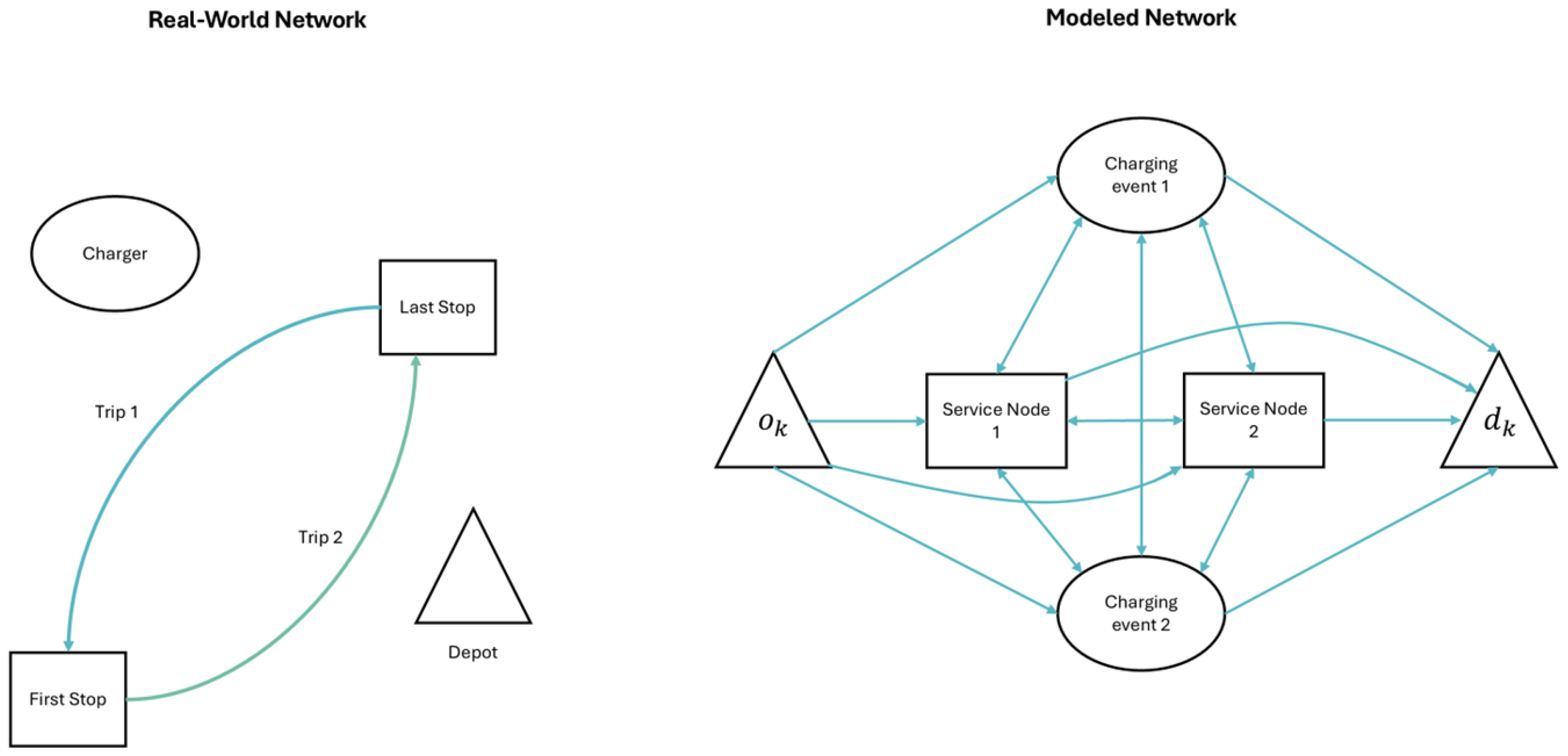
To provide an example, the translation of a real-world network with two trips, a depot, and a charging station is presented in Figure 1. In the modeled network, the depot is represented by two nodes: $o_k$ and $d_k$. The two trips are represented by the two service nodes, and the charger can offer two charging events, depicted as two different nodes in the modeled network.

Figure 1. Modeled network representation.

The main decision variables of this formulation include the following:

• $x_{ij}^k$: Binary flow variables, indicating the use of an arc $(i,j)\in A^k$ by a vehicle $k\in K$.
• $y_i^k$: Binary variables, indicating the use of a charging event $i\in F$ by a vehicle $k\in K$.
• $T_i^k$: Continuous variables, indicating the starting time of an event at a node $i\in N^k$.

At each service node $i\in V$, the completion of a trip incurs a travel cost ${\tilde{t}}_i,\forall i\in V$ (travel time, henceforth). The transit between the end location of a node $i\in N$ and the start location of a node $j\in N$ incurs a time cost $t_{ij}$. It is assumed that there are no movements made between source and charging nodes, as well as between sink and charging nodes.

Every vehicle $k\in K$ is assigned a continuous variable $e_i^k$ which denotes the SoC of the vehicle when it arrives at the node $i\in V^k\cup F\cup \left\{d_k\right\}$. Considering that all charging stations $z\in Z$ have the same and constant charging rate r and vehicle k arrives at the charging node $i\in F$ at time $T_i^k$ with SoC $e_i^k$, the vehicle requires a charging time of ${\tau }_i^k=({\varphi }_{max}^k-e_i^k)/r$ to recharge fully. Specifically, vehicle k is allowed to depart from the charging node after time $T_i^k+{\tau }_i^k$.

Additionally, every vehicle $k\in K$ is assigned a continuous variable ${\hat{e}}_i^k$ which denotes the SoC of the vehicle as it departs from the node $i\in V^k\cup F\cup \left\{o_k\right\}$. When the vehicle departs from its source node $o_k$, at the start of its shift, it applies that ${\hat{e}}_{o_k}^k={\varphi }_{max}^k$. At the remaining nodes $i\in V^k\cup F$, it applies that

$${\hat{e}}_i^k=e_i-g_i^k$$

where $g_i^k$ is a continuous variable indicating the SoC change during the visit of a vehicle k at the node $i\in V^k\cup F$.

At service nodes $i\in V^k$, the SoC of the vehicle k, while performing the corresponding trip, changes by $g_i^k={\eta }_i\ge 0$. Specifically, ${\eta }_i,\forall i\in V$ is a predefined parameter that, in the case of this study, depends on the length of the trip. At charging nodes $i\in F$, the vehicle recharges fully. Thus, it applies that

$$g_i^k=e_i^k-{\varphi }_{max}^k$$

A vehicle $k\in K$ is allowed to transit through an arc $(i,j)\in A^k$ if and only if its SoC is sufficient during its arrival at the node j, namely if $e_j^k\ge {\varphi }_{min}^k$. At the same arc $(i,j)$, the continuous variable ${\theta }_{ij}$ is assigned, which denotes the change in the SoC of vehicle k, when it transits between the end location of the node i and the start location of the node j.

The operational costs are defined as the sum of the two following terms:

• The operational costs for a vehicle $k\in K$ for its transit through the arc $(i,j)\in A^k$, without waiting at the start location of the node j, denoted by the parameter $b_{ij}$.
• The unit vehicle dwell cost, denoted by the parameter $\lambda$. That parameter, in turn, is multiplied by the difference between the starting time of the task at the node j (of the corresponding arc) and the time by which the vehicle k will have arrived at the start location of the node j:

  –

  $\lambda (T_j^k-T_i-{\tilde{t}}_i^k-t_{i}j),\forall k\in K,\forall (i,j)\in A^k|i\in V^k-\left\{j\right\}$.

  –

  $\lambda (T_j^k-T_i-{\tau }_i^k-t_{ij}),\forall k\in K,\forall (i,j)\in A^k|i\in F-\left\{j\right\}$.

  –

  $\lambda (T_j^k-T_i-t_{ij}),\forall k\in K,\forall (i,j)\in A^k|i=o_k$.

The resulting product is the operational cost of the vehicle k waiting at node j, until the task at the same node commences.

3.2. Extension of the MDEVSPTW Considering Travel Time Uncertainty

The above problem formulation assumes that the travel times ${\tilde{t}}_i$ at service nodes do not display variability but remain constant. However, as it is mentioned in the relevant literature review section, bus travel times do exhibit variability because of the operation of buses in mixed traffic conditions. The following reformulation aims to address this issue. Let S be the set that contains all possible scenarios with travel time values, where each outcome $s\in S$ has the same probability of actualization. The set S is developed by assuming that travel times follow the log-normal distribution, which is the most common assumption in past studies [49,50]. Consequently, it follows that the natural logarithms (logarithms, henceforth) of the travel times follow the normal distribution, with a mean value ${\mu }_i$ and a standard deviation ${\xi }_i$. By developing the set S with possible travel time values, for each scenario $s\in S$, we have a different travel time ${\tilde{t}}_i^s$ at each service node $i\in V$.

The introduction of multiple outcomes for travel times requires changes in the arc definitions of our network, as there cannot exist multiple outcomes for arcs $(i,j)\in A_3^k\cup A_4^k$, since the stochasticity of arc transit time $t_{ij}$ was not considered in past studies. Consequently, service node travel times cannot be used in the definition of arcs, thus resulting in a less exclusive definition, as follows:

• $A_3^k=(i,j)$, for all $i\in V^k$, for all $j\in V^k-\left\{i\right\}|l_i+t_{ij}\le u_j$.
• $A_4^k=(i,j)$, for all $i\in V^k$, for all $j\in F|l_i+t_{ij}\le u_j$.

Thus, the set of feasible arcs in our revised formulation is defined as follows:

$$\begin{array}{cc}{A}^k=& \left\{\begin{array}{c}{A}_1^k=(o_k,j),\forall j\in N^k-\left\{o_k\right\}\mid l_{o_k}+t_{o_{k}j}\le u_j\\ A_2^k=(j,d_k),\forall j\in N^k-\{o_k,d_k\}\\ A_3^k=(i,j),\forall i\in V^k,\forall j\in V^k-\left\{i\right\}\mid l_i+t_{ij}\le u_j\\ A_4^k=(i,j),\forall i\in V^k,\forall j\in F\mid l_i+t_{ij}\le u_j\\ A_5^k=(i,j),\forall i\in F,\forall j\in V^k\mid l_i+t_{ij}\le u_j\end{array}\right.\end{array}$$

The introduction of travel time variability aims to help create robust bus routing schedules, with good performance in extreme scheduling conditions (large disruptions/delays), while adhering to the scheduling problem constraints (keeping operations at acceptable levels of service). The required nomenclature for the formulation of the problem is provided in Table 2.

Table 2. Problem formulation nomenclature.

Sets
K	Set of available vehicles
Z	Set of charging stations
$O,D$	Set of source and sink nodes
V	Set of trips
$V^k$	Subset of scheduled trips that can be performed by vehicle k
F	Set of charging events
$F_0$	$F_0\subseteq F$ set of all possible charging events after removing the latest possible charging event at every charger
$F^z$	Subset of charging events at charger $z\in Z$ ordered chronologically from first to last
N	Set of all possible nodes, $N=\{V\cup F\cup O\cup D\}$
$N^k$	Subset of nodes associated with vehicle k, $V^k\cup F\cup \{o_k,d_k\}$
$A^k$	Set of feasible arcs for vehicle $k\in K$
$G^k$	Network associated with vehicle k, $G^k=(N^k,A^k)$
S	Set containing all travel time scenarios, generated by sampling with the use of a log-normal distribution
Parameters
$o_k,d_k$	Source and sink nodes associated with the depot of vehicle k
$[l_i,u_i]$	Time window associated with node $i\in N$
$t_{ij}$	Elapsed time on arc $(i,j)$, which is equal to the travel time between the end location at node $i\in N$ and the start location at node $j\in N$
${\tilde{t}}_i^s$	Travel time at service node $i\in V$ according to scenario $s\in S$
${\mu }_i$	Mean value of the probability distribution of the logarithms of the possible travel times at service node $i\in V$
${\xi }_i$	Standard deviation of the probability distribution of the logarithms of the possible travel times at service node $i\in V$
$\lambda$	Unit vehicle dwell cost
$b_{ij}^k$	Operational costs for a vehicle $k\in K$ using arc $(i,j)\in A^k$
${\varphi }_{max}^k$	SoC of vehicle k when fully charged
${\varphi }_{min}^k$	Minimum allowed SoC for vehicle k
r	Charging rate
${\eta }_i$	Consumed energy for performing trip $i\in V$
${\theta }_{ij}$	Consumed energy of vehicle $k\in K$ on arc $(i,j)\in A^k$
M	A very large positive number
$q_j$	Vector mapping the closest charging event location $q_j\in F$ to the end location at service node $j\in V$
${\omega }_i$	Vector mapping the charging event following a charging event $i\in F^z$ at a charging station $z\in Z$
Variables
$e_i^k$	SoC of vehicle k when arriving at node $i\in V^k\cup F\cup \left\{d_k\right\}$
${\overline{e}}_i^k$	SoC of vehicle k when completing a task at node $i\in V^k\cup F\cup \left\{o_k\right\}$
${\tau }_i^k$	Required time to recharge vehicle k at charging event $i\in F$
$g_i^k$	SoC change of vehicle k when performing task $i\in V^k\cup F$
$x_{ij}^k$	Binary variables, where $x_{ij}^k=1$ if vehicle k uses arc $(i,j)\in A^k$, and 0 otherwise
$y_i^k$	Binary variables, where $y_i^k=1$ if charging event $i\in F$ is performed by vehicle k, and 0 otherwise
${\sigma }_{ij}^k$	Continuous variables corresponding to arcs $(i,j)\in A^k,k\in K$
${\overline{\sigma }}_{ij}^k$	Continuous variables corresponding to arcs $(i,j)\in A^k,k\in K$, used for maintaining linearity of the constraints pertaining to vehicle energy consumption
$T_i^k$	Time when the task commences at node $i\in N^k$. $T_{o_k}^k$ indicates the departure time from a depot, $T_{d_k}^k$ the arrival time at a depot, and $T_i^k$ the time that a task begins at any other node $i\in V^k\cup F$
$z_{ij}^{ks}$	Continuous variables indicating the operational costs, for the travel time scenario $s\in S$ of a vehicle $k\in K$, using arc $(i,j)\in A^k|i\in V^k\cup F\cup o_k$

The aim of this model formulation is the minimization of the mean value of the possible operational costs $z_{ij}^{ks}$, $k\in K,(i,j)\in A^k|i\in V^k\cup F\cup o_k$ including the transit and dwell costs and considering all possible travel time scenarios $s\in S$. Consequently, the objective function is defined as follows:

$$\begin{array}{cc}\hfill & min{\displaystyle \frac{1}{\left|S\right|}}\left\{\sum _{s\in S}\sum _{k\in K}\sum _{\begin{array}{c}(i,j)\in A_k\\ i\in V^k\cup F\end{array}}{z}_{ij}^{ks}\right\}\hfill \end{array}$$

(1)

The operational costs $z_{ij}^{ks}$ are defined with the following constraints:

$$\begin{array}{c}\hfill z_{ij}^{ks}=\left\{\begin{array}{cc}(b_{ij}^k+\lambda (T_j^k-T_i^k-{\tilde{t}}_i^s-t_{ij}))x_{ij}^k,\hfill & \forall k\in K,\forall s\in S,(i,j)\in A_k\mid i\in V^k\hfill \\ (b_{ij}^k+\lambda (T_j^k-T_i^k-{\tau }_i^k-t_{ij}))x_{ij}^k,\hfill & \forall k\in K,\forall s\in S,(i,j)\in A_k\mid i\in F\hfill \\ (b_{ij}^k+\lambda (T_j^k-T_i^k-t_{ij}))x_{ij}^k,\hfill & \forall k\in K,\forall s\in S,(i,j)\in A_k\mid i=o_k\hfill \end{array}\right.\end{array}$$

(2)

which are nonlinear. To linearize them, one can replace them with the following equisatisfiable constraints:

$$\begin{array}{cc}\hfill & z_{ij}^{ks}\le x_{ij}^{k}M,\forall k\in K,\forall s\in S,(i,j)\in A_k\mid i\in V^k\cup F\cup \left\{o_k\right\}\hfill \end{array}$$

(3)

$$\begin{array}{cc}\hfill & z_{ij}^{ks}\ge -x_{ij}^{k}M,\forall k\in K,\forall s\in S,(i,j)\in A_k\mid i\in V^k\cup F\cup \left\{o_k\right\}\hfill \end{array}$$

(4)

$$\begin{array}{cc}\hfill & z_{ij}^{ks}\le b_{ij}^k+\lambda (T_j^k-T_i^k-{\tilde{t}}_i^s-t_{ij})+M(1-x_{ij}^k),\forall k\in K,\forall s\in S,(i,j)\in A_k\mid i\in V^k\hfill \end{array}$$

(5)

$$\begin{array}{cc}\hfill & z_{ij}^{ks}\le b_{ij}^k+\lambda (T_j^k-T_i^k-{\tau }_i^k-t_{ij})+M(1-x_{ij}^k),\forall k\in K,\forall s\in S,(i,j)\in A_k\mid i\in F\hfill \end{array}$$

(6)

$$\begin{array}{cc}\hfill & z_{ij}^{ks}\le b_{ij}^k+\lambda (T_j^k-T_i^k-t_{ij})+M(1-x_{ij}^k),\forall k\in K,\forall s\in S,(i,j)\in A_k\mid i=o_k\hfill \end{array}$$

(7)

$$\begin{array}{cc}\hfill & z_{ij}^{ks}\ge b_{ij}^k+\lambda (T_j^k-T_i^k-{\tilde{t}}_i^s-t_{ij})-M(1-x_{ij}^k),\forall k\in K,\forall s\in S,(i,j)\in A_k\mid i\in V^k\hfill \end{array}$$

(8)

$$\begin{array}{cc}\hfill & z_{ij}^{ks}\ge b_{ij}^k+\lambda (T_j^k-T_i^k-{\tau }_i^k-t_{ij})-M(1-x_{ij}^k),\forall k\in K,\forall s\in S,(i,j)\in A_k\mid i\in F\hfill \end{array}$$

(9)

$$\begin{array}{cc}\hfill & z_{ij}^{ks}\ge b_{ij}^k+\lambda (T_j^k-T_i^k-t_{ij})-M(1-x_{ij}^k),\forall k\in K,\forall s\in S,(i,j)\in A_k\mid i=o_k\hfill \end{array}$$

(10)

In addition, the following constraints perform the assignment of vehicles:

$$\begin{array}{cc}\hfill & \sum _{k\in K}\sum _{i:(i,j)\in A_k}{x}_{ij}^k=1,\forall j\in V\hfill \end{array}$$

(11)

$$\begin{array}{cc}\hfill & \sum _{k\in K}\sum _{i:(i,j)\in A_k}{x}_{ij}^k\le 1,\forall j\in F\hfill \end{array}$$

(12)

$$\begin{array}{cc}\hfill & \sum _{j:(o_k,j)\in A^k}{x}_{o_k,j}^k=\sum _{i:(i,d_k)\in A^k}{x}_{i,d_k}^k=1,\forall k\in K\hfill \end{array}$$

(13)

$$\begin{array}{cc}\hfill & \sum _{i:(i,j)\in A^k}{x}_{ij}^k-\sum _{i:(j,i)\in A^k}{x}_{ji}^k=0,\forall k\in K,\forall j\in V^k\cup F\hfill \end{array}$$

(14)

$$\begin{array}{cc}\hfill & l_i\le T_i^k\le u_i,\forall k\in K,\forall i\in N^k\hfill \end{array}$$

(15)

$$\begin{array}{cc}\hfill & x_{ij}^k\in \{0,1\},\forall k\in K,\forall (i,j)\in A^k\hfill \end{array}$$

(16)

$$\begin{array}{cc}\hfill & T_i^k+{\tilde{t}}_i^s+t_{ij}-T_j^k+{\sigma }_{ij}^k\le 0,\forall k\in K,\forall s\in S,\forall (i,j)\in A^k\mid i\in V^k\hfill \end{array}$$

(17)

$$\begin{array}{cc}\hfill & T_{o_k}^k+t_{o_{k}j}-T_j^k+{\sigma }_{o_{k}j}^k\le 0,\forall k\in K,\forall (o_k,j)\in A^k\hfill \end{array}$$

(18)

$$\begin{array}{cc}\hfill & T_i^k+{\tau }_i^k+t_{ij}-T_j^k+{\sigma }_{ij}^k\le 0,\forall k\in K,\forall (i,j)\in A^k\mid i\in F\hfill \end{array}$$

(19)

$$\begin{array}{cc}\hfill & {\sigma }_{ij}^k\le M(1-x_{ij}^k),\forall k\in K,\forall (i,j)\in A^k\hfill \end{array}$$

(20)

$$\begin{array}{cc}\hfill & {\sigma }_{ij}^k\ge -M(1-x_{ij}^k),\forall k\in K,\forall (i,j)\in A^k\hfill \end{array}$$

(21)

$$\begin{array}{cc}\hfill & T_i^k+{\tilde{t}}_i^s+t_{ij}\le u_j+M(1-x_{ij}^k),\forall k\in K,\forall s\in S,\forall i\in V^k,j\in V^k\cup F\cup \left\{d_k\right\}-\left\{i\right\}\hfill \end{array}$$

(22)

$$\begin{array}{cc}\hfill & T_i^k+{\tau }_i+t_{ij}\le u_j+M(1-x_{ij}^k),\forall k\in K,\forall i\in F,j\in V^k\cup F\cup \left\{d_k\right\}\hfill \end{array}$$

(23)

Constraint (11) ensures that every service node $j\in V$ will be matched with exactly one vehicle $k\in K$. Constraint (12) ensures that every charging event $j\in F$ will be matched with at most one vehicle $k\in K$. Constraint (13) ensures that every vehicle $k\in K$ will start and end its shift at the same depot. Constraint (14) ensures that if an arc $(i,j)$ that terminates at a service node or charging event is used by a vehicle $k\in K$, then the opposite arc $(j,i)$ will be declared as being used by the same vehicle k. Similarly, if an arc $(i,j)$ of the same type is not being used by a vehicle, then the opposite arc $(j,i)$ will be declared as not being used. Constraint (15) ensures that task start time at a node $i\in N^k$, for a vehicle $k\in K$, will start inside the corresponding time window $[l_i,u_i]$. Constraint (16) ensures that the variables $x_{ij}$ take on binary values.

Constraints (17) up to (21) are the linearized form of the following constraints:

$$\begin{array}{cc}\hfill & x_{ij}^k\left(T_i^k+{\tilde{t}}_i^s+t_{ij}\right)\le x_{ij}^k{T}_j^k,\forall s\in S,\forall k\in K,\forall (i,j)\in A^k\mid i\in V^k\hfill \end{array}$$

(24)

$$\begin{array}{cc}\hfill & x_{o_{k}j}^k\left(T_{o_k}^k+t_{o_{k}j}\right)\le x_{o_{k}j}^k{T}_j^k,\forall k\in K,\forall (o_k,j)\in A^k\hfill \end{array}$$

(25)

$$\begin{array}{cc}\hfill & x_{ij}^k\left(T_i^k+{\tau }_i^k+t_{ij}\right)\le x_{ij}^k{T}_j^k,\forall k\in K,\forall (i,j)\in A^k\mid i\in F\hfill \end{array}$$

(26)

These constraints ensure that a vehicle $k\in K$ will have arrived at the starting location of the node $j\in N^k-o_k$ before time $T_j^k$, at which the task at node j begins.

Constraints (22) and (23) ensure that the vehicle $k\in K$ will arrive at the start location of the node $j\in N^k-o_k$, before the upper time limit $u_j$ of the time window for the start of the task at node j.

The following constraints manage the vehicle battery $SoC$ variations and perform the charging scheduling:

$$\begin{array}{cc}\hfill & {\tau }_i^k={\displaystyle \frac{{\varphi }_{\max }^k-e_i^k}{r}},\forall i\in F,\forall k\in K\hfill \end{array}$$

(27)

$$\begin{array}{cc}\hfill & {\overline{e}}_{o_k}^k={\varphi }_{\max }^k,\forall k\in K\hfill \end{array}$$

(28)

$$\begin{array}{cc}\hfill & {\overline{e}}_j^k=e_i^k-g_j^k,\forall j\in V^k\cup F,\forall k\in K\hfill \end{array}$$

(29)

$$\begin{array}{cc}\hfill & g_i^k={\eta }_i,\forall i\in V^k,\forall k\in K\hfill \end{array}$$

(30)

$$\begin{array}{cc}\hfill & g_i^k=e_i^k-{\varphi }_{\max }^k,\forall i\in F,\forall k\in K\hfill \end{array}$$

(31)

$$\begin{array}{cc}\hfill & {\varphi }_{\min }^k\le e_j^k,\forall k\in K,\forall j\in V^k\cup F\cup \left\{d_k\right\}\hfill \end{array}$$

(32)

$$\begin{array}{cc}\hfill & e_j^k\le ({\overline{e}}_i^k-{\theta }_{ij})+(1-x_{ij}^k)M,\forall (i,j)\in A^k,\forall k\in K\hfill \end{array}$$

(33)

$$\begin{array}{cc}\hfill & e_j^k\ge ({\overline{e}}_i^k-{\theta }_{ij})+{\overline{\sigma }}_{ij}^k,\forall (i,j)\in A^k,\forall k\in K\hfill \end{array}$$

(34)

$$\begin{array}{cc}\hfill & {\overline{\sigma }}_{ij}^k\le M(1-x_{ij}^k),\forall (i,j)\in A^k,\forall k\in K\hfill \end{array}$$

(35)

$$\begin{array}{cc}\hfill & {\overline{\sigma }}_{ij}^k\ge -M(1-x_{ij}^k),\forall (i,j)\in A^k,\forall k\in K\hfill \end{array}$$

(36)

$$\begin{array}{cc}\hfill & y_i^k=\sum _{j:(i,j)\in A_k}{x}_{ij}^k,\forall i\in F,\forall k\in K\hfill \end{array}$$

(37)

$$\begin{array}{cc}\hfill & T_i^{k_0}+{\tau }_i^{k_0}+{\tilde{\sigma }}_i^{k_0}\le T_{{\omega }_i}^k+M\left(1-\sum _{\rho :({\omega }_i,\rho )\in A^k}{x}_{{\omega }_i\rho }^k\right),\forall i\in F_0,\forall k\in K,\forall k_0\in K\hfill \end{array}$$

(38)

$$\begin{array}{cc}\hfill & {\tilde{\sigma }}_i^{k_0}\le M(1-y_i^{k_0}),\forall i\in F_0,\forall k_0\in K\hfill \end{array}$$

(39)

$$\begin{array}{cc}\hfill & {\tilde{\sigma }}_i^{k_0}\ge -M(1-y_i^{k_0}),\forall i\in F_0,\forall k_0\in K\hfill \end{array}$$

(40)

$$\begin{array}{cc}\hfill & e_j^k\le {\varphi }_{\max }^k,\forall k\in K,\forall j\in V^k\cup F\cup \left\{d_k\right\}\hfill \end{array}$$

(41)

$$\begin{array}{cc}\hfill & {\overline{e}}_j^k\ge {\varphi }_{\min }^k+{\theta }_{j,q_j},\forall j\in K,\forall j\in V^k\hfill \end{array}$$

(42)

$$\begin{array}{cc}\hfill & \sum _{k\in K}{y}_i^k{l}_i\le T_{{\omega }_i}^k+M\left(1-\sum _{\rho :({\omega }_i,\rho )\in A^k}{x}_{{\omega }_i\rho }^k\right),\forall i\in F_0,\forall k\in K\hfill \end{array}$$

(43)

Constraint (27) defines the charging rate of a vehicle $k\in K$, during a charging event $i\in F$. Constraint (28) ensures that a vehicle $k\in K$ leaves its depot/departs from its source node $o_k$ fully charged. Constraint (29) defines the $SoC$ variation of a vehicle $k\in K$, when it performs a task at a node $i\in V^k\cup F$. Constraint (30) defines the $SoC$ variation of a vehicle $k\in K$, when it performs a trip at a service node $i\in V^k$. Constraint (31) defines the $SoC$ variation of a vehicle $k\in K$, when it recharges during a charging event $i\in F$. Constraint (32) ensures that the $SoC$ of a vehicle $k\in K$ remains above its minimum allowed $SoC$ level ${\varphi }_{min}^k$ throughout the duration of its shift. Constraints (33) up to (36) are the linearized form of the following constraint:

$$\begin{array}{c}\hfill e_j^k\ge ({\overline{e}}_i^k-{\theta }_{ij})x_{ij}^k,\forall (i,j)\in A^k,\forall k\in K\end{array}$$

(44)

These constraints define the SoC variation of a vehicle $k\in K$, when it transits through an arc $(i,j)\in A^k$.

The following constraints involve the reduction in conflicting arcs:

$$\begin{array}{cc}\hfill & x_{ij}^k+x_{ij}^{k^{\prime }}\le 1,\forall k\in K,\forall k^{\prime }\in K-\left\{k^{\prime }\right\},\forall (i,j)\in A_k\cap A_{k^{\prime }}\hfill \end{array}$$

(45)

$$\begin{array}{cc}\hfill & x_{ij}^k+x_{i^{\prime }{j}^{\prime }}^k\le 1,\forall k\in K,\forall (i,j)\in A_k,\forall (i^{\prime },j^{\prime })\in A_k:i^{\prime }=i\wedge j^{\prime }\ne j\hfill \end{array}$$

(46)

$$\begin{array}{cc}\hfill & x_{ij}^k+x_{i^{\prime }{j}^{\prime }}^k\le 1,\forall k\in K,\forall (i,j)\in A_k,\forall (i^{\prime },j^{\prime })\in A_k:i^{\prime }\ne i\wedge j^{\prime }=j\hfill \end{array}$$

(47)

Let $i,j,k$ and $i^{\prime },j^{\prime },k^{\prime }$ be two adjacent arcs of the polygraph G. It is assumed that these arcs are in conflict if $k=k^{\prime }$ or $i=i^{\prime }$ or $j=j^{\prime }$. These arcs are removed with the valid inequalities described in the constraints (38)–(40).

3.3. Extension of the MDEVSPTW, Considering Travel Time Stochasticity and a Chance Constraint

Satisfying all constraints of every service node for all possible travel time outcomes leads to the creation of robust schedules. However, these schedules have higher operational costs, as extreme outcomes of travel times (meaning large delays) may have an outsized contribution to increasing mean operational costs. Consequently, the conversion of a constraint into a chance constraint is investigated, with the aim of observing the change in operational costs in relation to the probability value of the chance constraint.

The constraint which is converted into a chance constraint is constraint (17):

$$\begin{array}{c}\hfill T_i^k+{\tilde{t}}_i^s+t_{ij}-T_j^k+{\sigma }_{ij}^k\le 0,\forall k\in K,\forall s\in S,\forall (i,j)\in A^k\mid i\in V^k\end{array}$$

(48)

The introduction of stochasticity in travel times allows for the investigation of the effects on operational costs of the untimely start or cancellation of tasks at the node j after the arc $(i,j)\in A^k$ due to large travel time delays at the previous node $i\in V^k$. The chance constraint is defined as follows:

$$\begin{array}{c}\hfill \mathrm{Prob}\left(T_i^k+{\tilde{t}}_i^s+t_{ij}-T_j^k+{\sigma }_{ij}^k\le 0\right)\le \alpha ,\forall k\in K,\forall s\in S,\forall (i,j)\in A^k\mid i\in V^k,\alpha \in [0,1]\end{array}$$

(49)

where $\alpha$ is the parameter that determines the probability of the constraint realization.

The above defined form of the constraint cannot be modeled on a commercial solver. However, since the term ${\tilde{t}}_i^s$ is not multiplied by any other variable, it follows that at a service node $i\in V^k$, with $s\in S$ travel time outcomes, constraint (49) is realized for the $[\alpha ,|S\left|\right]$ lowest travel times ${\tilde{t}}_i^s$. This is true because as the value of ${\tilde{t}}_i^s$ increases, the left term of the inequality equation of the probability term also increases. Thus, the chance constraint is less likely to be realized.

The final form of the chance constraint is the following:

$$\begin{array}{c}\hfill T_i^k+{\tilde{t}}_i^s+t_{ij}-T_j^k+{\sigma }_{ij}^k\le 0,\forall k\in K,\forall (i,j)\in A^k\mid i\in V^k,\forall s\in S_i^{\alpha }\end{array}$$

(50)

where $S_i^{\alpha }$ is a subset of S, which contains the outcomes $s\in S$ that correspond to the $[\alpha ,|S\left|\right]$ lowest travel times ${\tilde{t}}_i^s$ at the service node $i\in V^k$.

The formulation of this version of the problem contains the initial objective function:

$$\begin{array}{c}\hfill \min {\displaystyle \frac{1}{\left|S\right|}}\sum _{s\in S}\sum _{k\in K}\sum _{(i,j)\in A_k\mid i\in V^k\cup F}{z}_{ij}^{ks}\end{array}$$

(51)

under the constraints (3)–(16), (18)–(47) and (50).

4. Numerical Experiments

In the numerical experiments, we present the results of the implementation of our model. We are considering four scheduling cases $(A,B,C,D)$ with respect to the timetable of the examined network. The start and end node locations for every case examined are distributed on a $60\times 60$ km grid. Every scheduling case consists of 10 service trips $V=1,2,3,4,5,6,7,8,9,10$ on random lines, two charging stations, and two vehicles $K=1,2$. Four charging events correspond to every charger, with the charging events in total being defined as such: $F=1001,1011,1021,1031\cup 1002,1012,1022,1032$. In our code formulation, identifiers $1001,1011,1002,1012$, etc., represent the charging nodes. We implemented this coding logic to separate the charging nodes from other tasks, such as service trips V or the source and sink nodes $o1,o2,d1,d2$. As mentioned, in every examined case, there are two available charging stations. Hence, the identifiers of the charging nodes that end with the digit 1 correspond to the first charger, and those that end with the digit 2 correspond to the second charger. Moreover, it should be stated that in all the scheduling cases examined in this problem, all buses start their service at a source node, fully charged with their battery at its maximum capacity. A source node (start depot) corresponds to each vehicle $(o_1=11,o_2=21)$, as well as a sink node (end depot) $(d_1=12,d_2=22)$.

The start location coordinates of the nodes are identical to the end location coordinates. Additionally, every vehicle at the end of its shift returns to the same depot from where it started its shift. Thus, the source node $o_k$ of a vehicle $k\in K$ has the same coordinates as its sink node $d_k$. Moreover, the upper arrival time limit $u_{d_k}$ at the sink node $d_k$ of a vehicle k is always greater than the upper departure time limit $u_{o_k}$ from the source node $o_k$ of the same vehicle k, as it is not possible for a vehicle to have returned to its depot without it having started its shift. Furthermore, the lower departure time limit $l_{o_k}$ from the source node $o_k$ of the vehicle k and its corresponding lower arrival time limit $l_{d_k}$ at the sink node $d_k$ have values of zero. This occurs since there is the possibility of the vehicle k not needing to be deployed for service and thus remaining in its depot for the whole duration of the examined scheduling case. Consequently, there is the requirement for a virtual concurrent departure from and arrival to the depot of the vehicle k, at time $T_{o_k}=T_{d_k}=0$. The values of the node formulation described above for the source and sink nodes are presented in Table 3.

Table 3. Values of source and sink nodes; node location coordinates in kilometers; $l_i$, $u_i$ in minutes.

	Node Index	Start Node Latitude	Start Node Longitude	End Node Latitude	End Node Longitude	${\mathit{l}}_{\mathit{i}}$	${\mathit{u}}_{\mathit{i}}$
Case: A	11	56	1	56	1	0	480
	12	36	54	36	54	0	480
	21	56	1	56	1	0	1080
	22	36	54	36	54	0	1080
Case: B	11	17	24	17	24	0	480
	12	33	54	33	54	0	480
	21	17	24	17	24	0	1080
	22	33	54	33	54	0	1080
Case: C	11	58	28	58	28	0	480
	12	17	53	17	53	0	480
	21	58	28	58	28	0	1080
	22	17	53	17	53	0	1080
Case: D	11	2	10	2	10	0	480
	12	47	55	47	55	0	480
	21	2	10	2	10	0	1080
	22	47	55	47	55	0	1080

For every service node $i\in V$, the upper task start time limit $u_i$ is 400 min greater than the lower task start time limit $l_i$. For the travel time distribution parameters ${\mu }_i$ and ${\xi }_i$, publicly available GTFS (general transit feed specification) data from the public transport operator of Krakow (ZTP) are used.

The values of the node formulation described above for the source and sink nodes, the travel time distribution parameters ${\mu }_i$ and ${\xi }_i$, and the upper and lower charging event starting time limits $u_i$ and $l_i$, are presented in Table 4 and Table 5 below.

Table 4. Values of source and sink nodes; node location coordinates in kilometers; $l_i$, $u_i$ in minutes; ${\xi }_i$, $exp\left({\mu }_i\right)$ in seconds.

	Node Index	Start Node Latitude	Start Node Longitude	End Node Latitude	End Node Longitude	${\mathit{l}}_{\mathit{i}}$	${\mathit{u}}_{\mathit{i}}$	${\mathit{\xi }}_{\mathit{i}}$	$\mathbf{exp}({\mathit{\mu }}_{\mathit{i}}$)
Case: A	1	1	40	11	48	40	440	0.375	1239.332
	2	21	2	16	58	15	415	0.435	1316.820
	3	55	55	46	51	104	504	0.387	1191.878
	4	33	12	17	6	144	544	0.374	1027.800
	5	16	24	52	8	250	650	0.394	1219.124
	6	10	42	19	19	238	638	0.413	1716.638
	7	52	33	39	16	355	755	0.400	1101.319
	8	23	44	56	21	316	716	0.378	873.533
	9	17	36	33	11	446	846	0.373	749.333
	10	48	28	35	47	448	848	0.391	1050.491
Case: B	1	21	25	16	13	26	426	0.320	999.906
	2	29	17	16	1	26	426	0.395	1258.506
	3	21	57	36	48	114	514	0.325	1148.150
	4	22	14	17	15	150	550	0.345	1257.082
	5	18	41	38	25	228	628	0.438	1071.229
	6	19	13	2	57	236	636	0.363	1275.500
	7	20	33	19	49	324	724	0.400	1421.056
	8	23	45	30	36	321	721	0.350	2262.859
	9	53	31	39	56	402	802	0.474	1107.815
	10	27	27	10	5	409	809	0.383	630.5405
Case: C	1	52	58	12	38	22	422	0.433	1233.598
	2	54	4	43	31	16	416	0.396	1062.877
	3	44	24	30	55	158	558	0.356	650.622
	4	17	7	18	2	113	513	0.431	826.836
	5	40	28	20	32	202	602	0.384	1335.253
	6	49	36	20	44	231	631	0.488	839.893
	7	7	18	33	20	344	744	0.431	905.527
	8	41	29	32	33	313	713	0.406	1295.796
	9	37	41	30	55	429	829	0.426	1194.150
	10	51	29	4	20	459	859	0.413	1305.510
Case: D	1	46	8	11	50	52	452	0.442	1230.547
	2	37	58	17	33	51	451	0.375	772.440
	3	36	16	44	53	127	527	0.393	898.384
	4	48	22	4	41	125	525	0.402	1630.079
	5	39	11	22	6	245	645	0.423	844.820
	6	32	47	39	27	225	625	0.386	922.120
	7	37	7	40	13	336	736	0.417	1099.089
	8	16	27	44	14	330	730	0.420	1704.108
	9	14	24	47	57	423	823	0.386	1091.990
	10	10	49	24	32	443	843	0.434	1053.837

Table 5. Values of source and sink nodes representing the charging events; node location coordinates in kilometers; $l_i$, $u_i$ in minutes.

	Node Index	Start Node Latitude	Start Node Longitude	End Node Latitude	End Node Longitude	${\mathit{l}}_{\mathit{i}}$	${\mathit{u}}_{\mathit{i}}$
Case: A	1001	9	29	9	29	115	515
	1002	55	42	55	42	145	545
	1011	9	29	9	29	230	630
	1012	55	42	55	42	311	711
	1021	9	29	9	29	332	732
	1022	55	42	55	42	311	711
	1031	9	29	9	29	408	808
	1032	55	42	55	42	405	805
Case: B	1001	39	36	39	36	157	557
	1002	37	44	37	44	126	526
	1011	39	36	39	36	211	611
	1012	37	44	37	44	303	703
	1021	39	36	39	36	440	840
	1022	37	44	37	44	303	703
	1031	39	36	39	36	440	840
	1032	37	44	37	44	425	825
Case: C	1001	10	10	10	10	107	507
	1002	30	44	30	44	155	555
	1011	10	10	10	10	245	645
	1012	30	44	30	44	244	644
	1021	10	10	10	10	329	729
	1022	30	44	30	44	335	735
	1031	10	10	10	10	428	828
	1032	30	44	30	44	426	826
Case: D	1001	7	50	7	50	126	526
	1002	29	15	29	15	110	510
	1011	7	50	7	50	209	609
	1012	29	15	29	15	202	602
	1021	7	50	7	50	334	734
	1022	29	15	29	15	348	748
	1031	7	50	7	50	424	824
	1032	29	15	29	15	437	837

For every scheduling case, the following values are considered:

• Unit vehicle dwell cost $\lambda =2$ units/min.
• SoC of vehicle k when fully charged ${\varphi }_{max}^k=300$ energy units.
• Minimum allowed SoC level of vehicle k: ${\varphi }_{min}^k=10$ energy units.
• Unit travel cost = 10 cost units/km.
• Charging station charging rate r = 10 energy units/min.
• Unit energy consumption rate = 1.3 units/min.

As mentioned in the previous section, $\left|S\right|=100$ scenarios $s\in S$ of travel times ${\tilde{t}}_i^s$ are defined for each service trip $i\in V$. The outcomes are constructed with the following process: for every service trip $i\in V$, a sample of size $N=\left|S\right|$ is created that follows the normal distribution, with a mean value of ${\mu }_i$ and a standard deviation of ${\xi }_i$. For each outcome $s\in S$ of the above sample, Euler’s number $\left(e\right)$ is raised to the power of the corresponding value of the sample. The travel times ${\tilde{t}}_i^s$ of the service trip $i\in V$ are defined as the result of this computation. The energy consumption ${\eta }_i$ during the service trip $i\in V$ is defined as the product of the unit energy consumption rate multiplied by the length of the Euclidean distance between the start and end locations of the relevant service node. The energy consumption ${\theta }_{ij}$ between the end location of the node $i\in N$ and the start location of the node $j\in N$, is also defined as the product of the unit energy consumption rate multiplied by the length of the Euclidean distance between the locations mentioned above.

Furthermore, each of the four scheduling cases is evaluated with three different methods:

• with |S| = 1 travel time scenario using the mean values of the travel times (deterministic approach).
• with |S| = 100 travel time scenarios.
• with |S| = 100 travel time scenarios and the chance constraint, where a = 80%.

In all cases, the model variants are solved with the commercial solver software Gurobi 11.0.0, implemented in Python 3. The computer on which the evaluations were performed is equipped with 16 GB of RAM, an Intel Core i5-1135G7 CPU with four cores, eight threads, and clock speeds ranging from 3.9 to 4.1 GHz during the execution of the relevant programs.

The results of the numerical experiments described above are presented in Table 5 and Table 6 and Figure 2, Figure 3 and Figure 4.

Table 6. Operational costs results by scheduling case and evaluation method (in cost units).

Scheduling Case	|S| = 1	|S| = 100 a = 100%	|S| = 100 a = 80%
A	1909	2847	2330
B	1478	2444	1925
C	2286	3348	2752
D	1505	2633	1995

Figure 2. Graphic representation of operational costs results by scheduling case and evaluation method (in cost units).

Figure 3. Graphic representation of percentage increase in operational costs compared to reference case by scheduling case and evaluation method.

Figure 4. Graphic representation of the increase in computational time results by scheduling case and evaluation method.

One can notice that the scheduling cases that are evaluated with multiple travel time outcomes result in schedules with higher operational costs. This is to be expected, as stochastic travel times contain extreme cases. Consequently, to accommodate these extreme cases, the schedules need to contain large time buffers in the operational schedules of electric buses, increasing operational costs. As shown in Figure 3, for the schedules where all constraints are respected, operational costs are increased between 49% and 75%. In the schedules where the chance constraint is introduced, and it is accepted that for 20% of the worst time travel outcomes there may be a delay or cancellation of a service at a node, the increase in operational costs is less severe (between 20% and 33%).

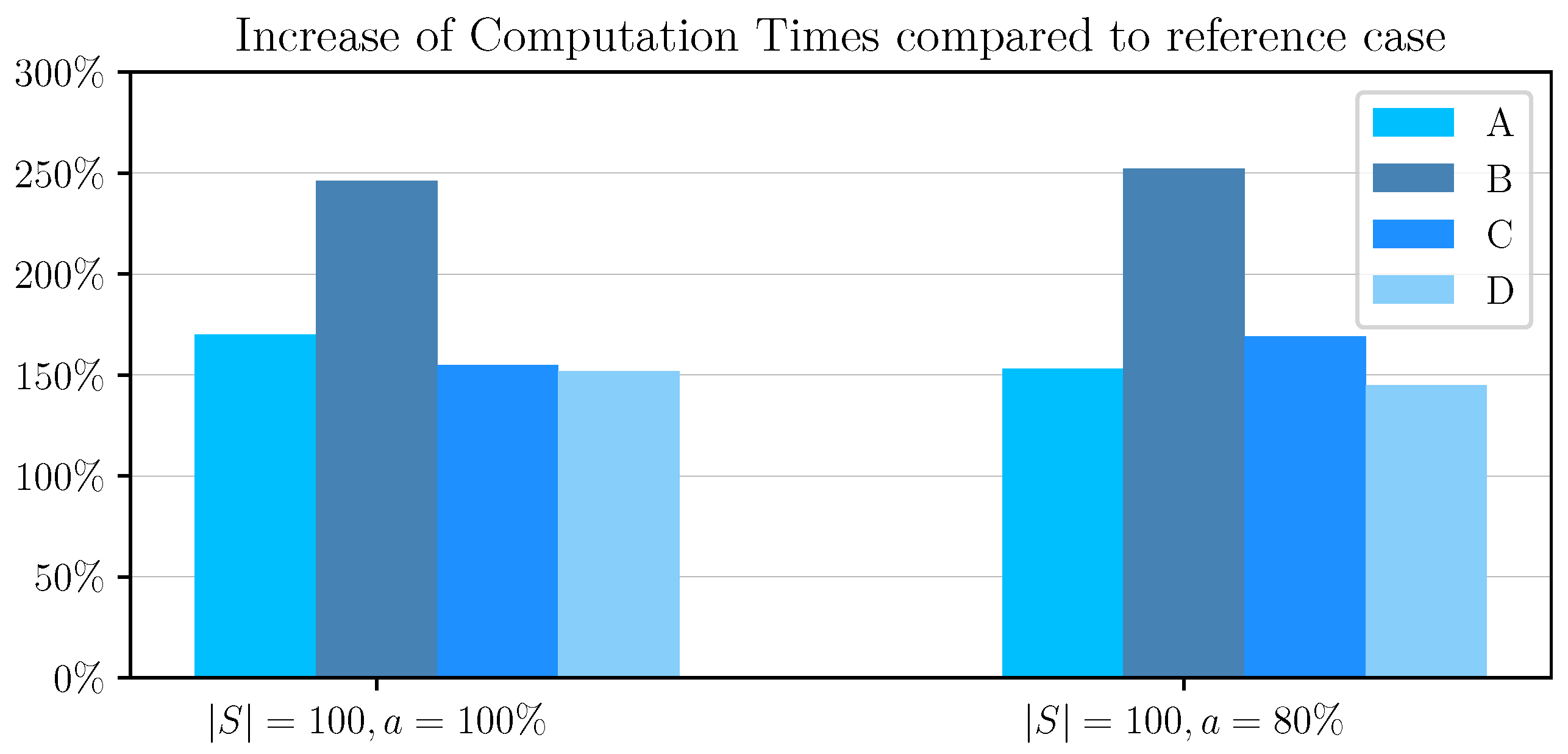
As presented in Table 7, when solving the stochastic optimization problem considering $\left|S\right|=100$ travel time outcomes, computation times are approximately 150 to 250 times greater than the corresponding computation times for solving the deterministic model ($\left|S\right|=1$). The use of the chance constraint does not significantly change the computation times compared to the case of not using the chance constraint, as we can also observe in Figure 4.

Table 7. Computation time results by scheduling case and evaluation method (in minutes).

Scheduling Case	|S| = 1	|S| = 100 a = 100%	|S| = 100 a = 80%
A	2.15	368.13	331.93
B	1.45	358.1	366.38
C	2.42	377.34	411.43
D	3.17	483.2	462.94

Sensitivity Analysis Based on the Variation in Travel Time Standard Deviation

The aim of this subsection is to investigate the variation in the operational costs of a schedule resulting from a scheduling case as the standard deviation of travel times ${\xi }_i$ changes. Thus, Monte Carlo simulations are performed according to the following equation:

$$\begin{array}{c}\hfill {\displaystyle \frac{1}{\left|S\right|}}(\sum _{s\in S}\sum _{k\in K}\sum _{(i,j)\in A_k|i\in V^k}\left(b_{ij}^k+\lambda (T_j^k-T_i^k-{\tilde{t}}_i^s-t_{ij})\right)x_{ij}^k\\ \hfill +\sum _{s\in S}\sum _{k\in K}\sum _{(i,j)\in A_k|i\in F}\left(b_{ij}^k+\lambda (T_j^k-T_i^k-{\tau }_i^k-t_{ij})\right)x_{ij}^k\\ \hfill +\sum _{s\in S}\sum _{k\in K}\sum _{(i,j)\in A_k|i=o_k}\left(b_{ij}^k+\lambda (T_j^k-T_i^k-t_{ij})\right)x_{ij}^k)\end{array}$$

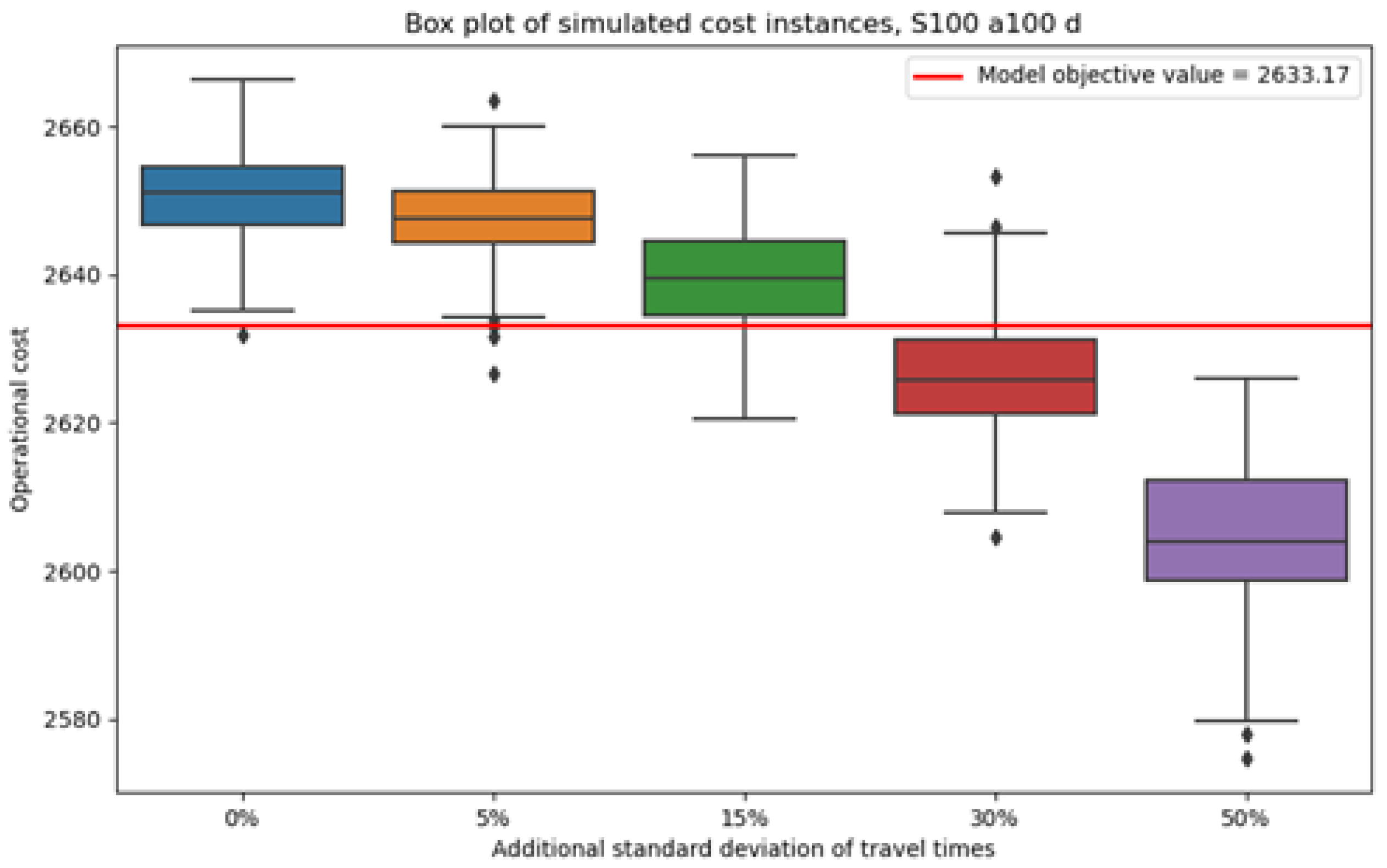
In more detail, for every schedule that was constructed considering stochastic travel times, 200 simulations are computed for a 0%, 5%, 15%, 30%, and 50% increase in the standard deviation of the natural logarithms of the service travel times.

In each simulation, 100 travel time outcomes are computed for each service node. The mean values of the normal distribution of the natural logarithms of the travel times are equal to those of the numerical experiment, while the standard deviations receive their respective increase. The seed value is random for each simulation. The values of the parameters $b_{ij}^k$, $\lambda$, $t_{ij}$ are identical to those of the numerical experiment, while for the parameters $T_i^k$,${\tau }_i^k$ and $x_{ij}^k$, the values of the corresponding decision variables are used from the evaluation results of the relevant schedule.

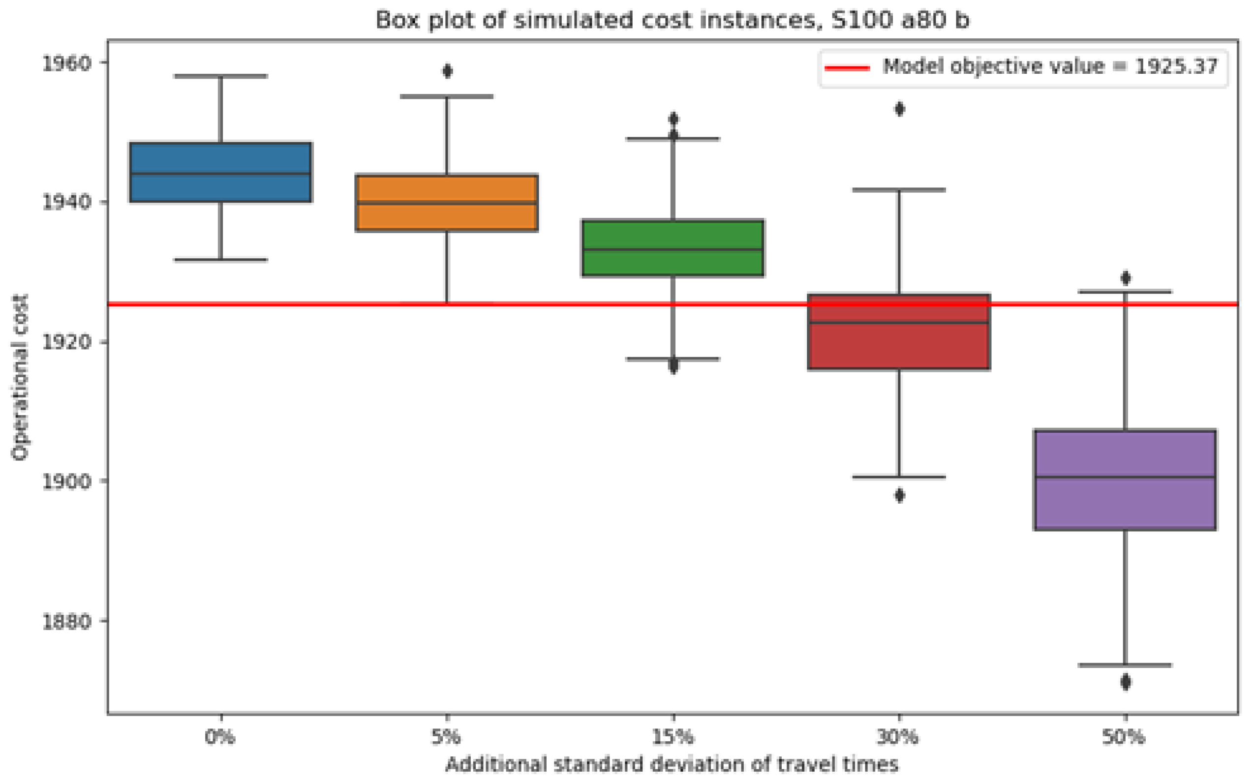
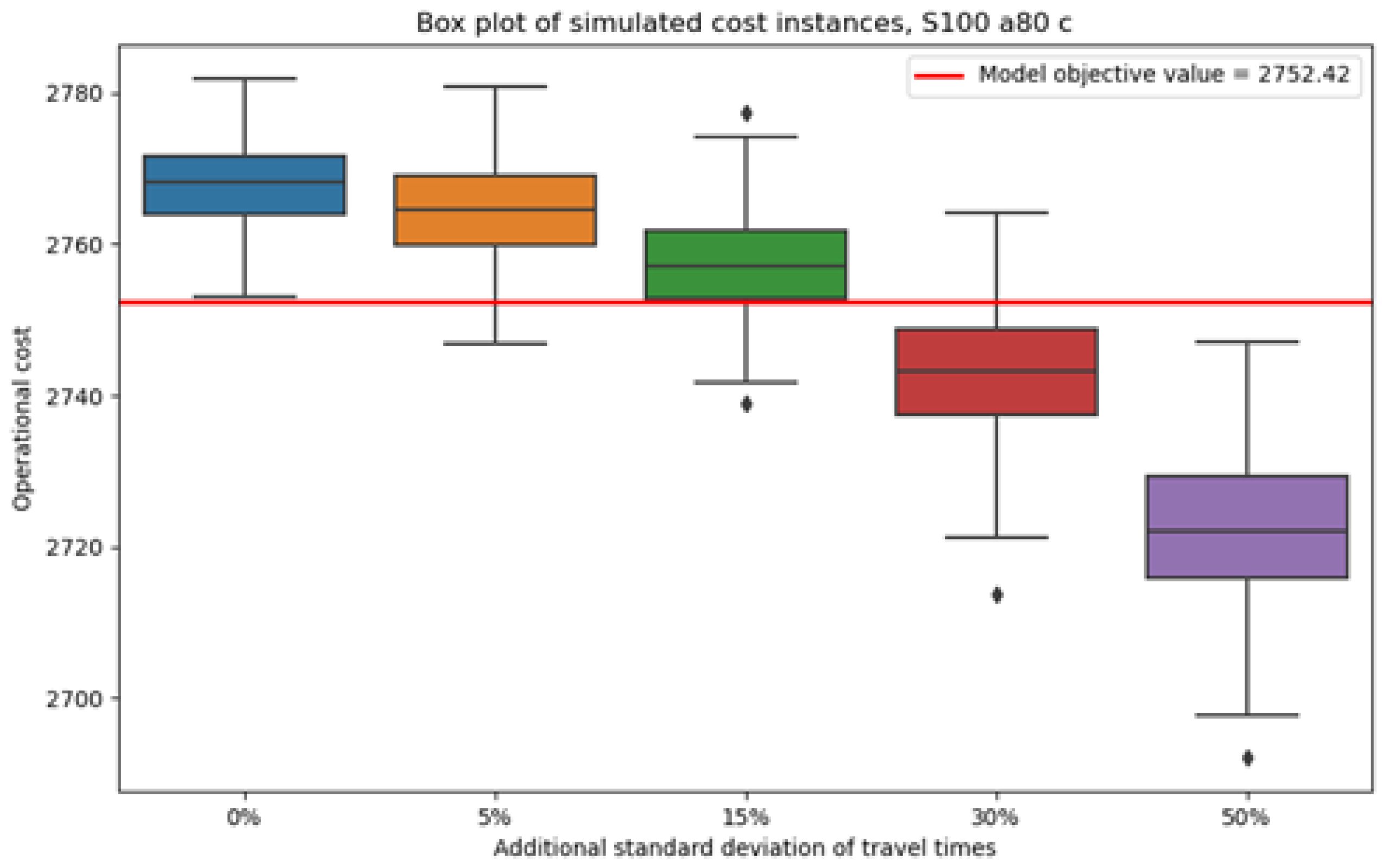
The box plots of the operational costs simulations are presented below in Figure 5, Figure 6, Figure 7, Figure 8, Figure 9, Figure 10, Figure 11 and Figure 12. In each case, the box is defined as the inter-quartile range (IQR) of the corresponding sample, while the whiskers extend to the values that have a $1.5\times$ IQR difference from the median. The median is shown as a black line that intersects the box and the outlier values are shown as diamond-shaped points.

Figure 5. Values of simulated operational costs for the schedule that corresponds to the scheduling case A and evaluation without the chance constraint.

Figure 6. Values of simulated operational costs for the schedule that corresponds to the scheduling case A and evaluation with the chance constraint.

Figure 7. Values of simulated operational costs for the schedule that corresponds to the scheduling case B and evaluation without the chance constraint.

Figure 8. Values of simulated operational costs for the schedule that corresponds to the scheduling case B and evaluation with the chance constraint.

Figure 9. Values of simulated operational costs for the schedule that corresponds to the scheduling case C and evaluation without the chance constraint.

Figure 10. Values of simulated operational costs for the schedule that corresponds to the scheduling case C and evaluation with the chance constraint.

Figure 11. Values of simulated operational costs for the schedule that corresponds to the scheduling case D and evaluation without the chance constraint.

Figure 12. Values of simulated operational costs for the schedule that corresponds to the scheduling case D and evaluation with the chance constraint.

According to the above results, for a certain schedule, if the increase in the standard deviation of the natural logarithms of the service travel times is less than 15%, then the change in operational costs is negligible. That is because the change in the median operational costs is around 10 cost units, which in all cases amounts to a change of less than 1%. However, the median operational costs do decrease exponentially as the standard deviation of service travel times increases; thus, for changes greater than 15%, the variations in operational costs stop being negligible. However, for an increase in the standard deviation performed in the present analysis, the change in the median operational costs remains small. In all cases, the standard deviation of the simulated operational costs does not vary considerably, and the inter-quartile ranges do not increase significantly as the standard deviation of the service travel time increases. Lastly, the simulated operational costs remain relatively similar to the operational costs that result from the evaluation of the numerical experiments.

5. Conclusions

The battery electric bus scheduling problem is complex, with many factors that must be taken into consideration. The most critical ones are the limited energy capacity of batteries and the time that is required to charge them. Additionally, there are matters such as passenger demand, road traffic uncertainties, and possible variations in energy costs during the day, which further complicate scheduling decisions.

This paper provides a MILP model with the goal of minimizing operational costs while considering time windows, multiple depots, and multiple charging stations, along with charging events. These time windows are available for charging the buses from the start of the operating time of the examined network, enabling us to explore the entire solution space to find the globally optimal solution without excluding any possible optimal results. Furthermore, valid inequalities are utilized for the reduction in the solution space. We assume stochastic travel times that follow the log-normal distribution. The aim of this is to construct schedules that provide transit operators with a service resilient to extreme conditions at a reasonable operational cost. If, however, a transit operator prefers reduced coverage in extreme events—without a total disregard for them—in exchange for a reduction in cost, then the variant of the model with the chance constraint can satisfy that demand. The chance constraint is formulated in a linear form, such that the model can be evaluated with a commercial solver.

The two variants of the model and the reference paper model are evaluated with indicative synthetic scheduling scenarios of 10 trips each. The variant of the model without the chance constraint produces schedules with operational costs $49\%$ to $75\%$ higher than the case where stochastic travel times are not considered. However, the variant of the model with the chance constraint and a probability value of $a=80\%$ (which means that there is a probability of $80\%$ that a trip starts with no delays) produces schedules with only $20\%$ to $33\%$ higher operational costs. At this point, it should be mentioned that the solution time for 100 outcomes for each trip travel time increases by approximately 150 to 250 times for both variants of the model compared to the reference model. Both variants of the model are sensitive to variations in travel times’ standard deviation, but the values of the mean operational costs do not vary significantly for reasonable variations in the travel times’ standard deviation. Indeed, the inclusion of travel time stochasticity in scheduling considerations increases operational costs. However, this method of scheduling reveals operational costs that are closer to the ones in real-life situations for transit operators that aim to achieve a high level of service, meaning smooth operation during unfavorable scheduling conditions. For transit operators that are more sensitive to operational costs but desire a level of coverage in unfavorable scheduling conditions, the variant of the model with the chance constraint provides a higher level of flexibility.

Electrical vehicle battery deterioration is a phenomenon that should be considered during the scheduling procedure and should affect the planning strategy for the implementation of electric buses in the public network. The developed model presented above strives to minimize the operational costs while taking into consideration the limitations of the energy level of the vehicles. In the case of electric vehicle battery deterioration, which arises after some years of the operation of the bus, the model would assign the bus for charging more often while also trying to minimize the itineraries required for charging. Certainly, after some years of battery deterioration, the operational cost would be increased, but again, it would be the minimum possible.

Considering the benefits for the users, the developed model—which handles the uncertainty regarding the travel times of the buses—could offer a more robust timetable for the examined network. Consequentially, the punctuality of the itineraries would be improved and the waiting time variation for the passengers would be decreased. This could also affect how trustworthy (reliable) passengers consider the bus network to be and would encourage them to use public transport more, hopefully leading to an environmentally friendly solution for this form of transportation.

In future research, our approach can also be applied to larger networks, examining its scalability and potential computational limits of the model.