

Benchmarking Methods for Pointwise Reliability

 , ,
, , 
Abstract
1. Introduction
2. Related Work
3. Methodology
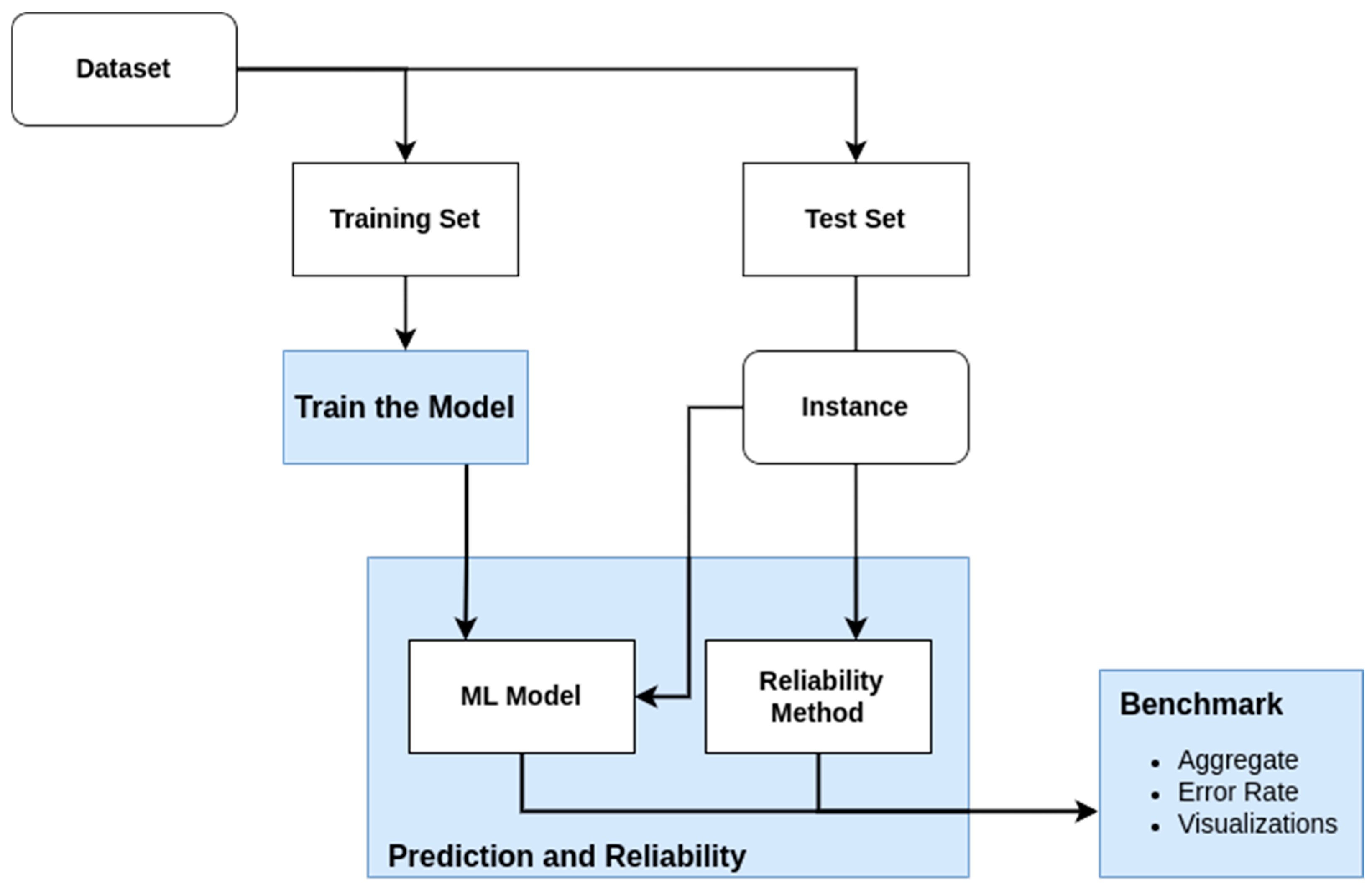
3.1. Benchmark
- Correct (0): true label 0 with correct prediction.
- Incorrect (0): true label 0 with incorrect prediction.
- Correct (1): true label 1 with correct prediction.
- Incorrect (1): true label 1 with incorrect prediction.
3.2. Dataset
3.3. Pointwise Reliability Methods
3.3.1. Subtractive Clustering
- Parameter Optimization: A grid search was performed over the parameter (starting with the values 0.05 and ending with 0.5, with 18 additional values in between) to maximize the number of valid clusters, ensuring that no cluster contained fewer than a predefined minimum number (3) of members.
- Clustering and Assignment: Using the optimal , the algorithm assigned each data point to the nearest cluster if it was within the range; otherwise, points were marked as unassigned.
- Reliability Computation: Reliability for each new instance is computed based on the following:
3.3.2. DBSCAN Method
- Parameter Optimization: A grid search was performed on the “eps” (10 values ranging from 0.01 to 0.5 in equal intervals) and “min samples” (4 values, starting at 2 and increasing by 2 in each iteration) to maximize the number of clusters.
- Clustering and Assignment: Using optimal parameters, DBSCAN assigned points to clusters or labeled them as noise.
3.3.3. Distance-Based Method
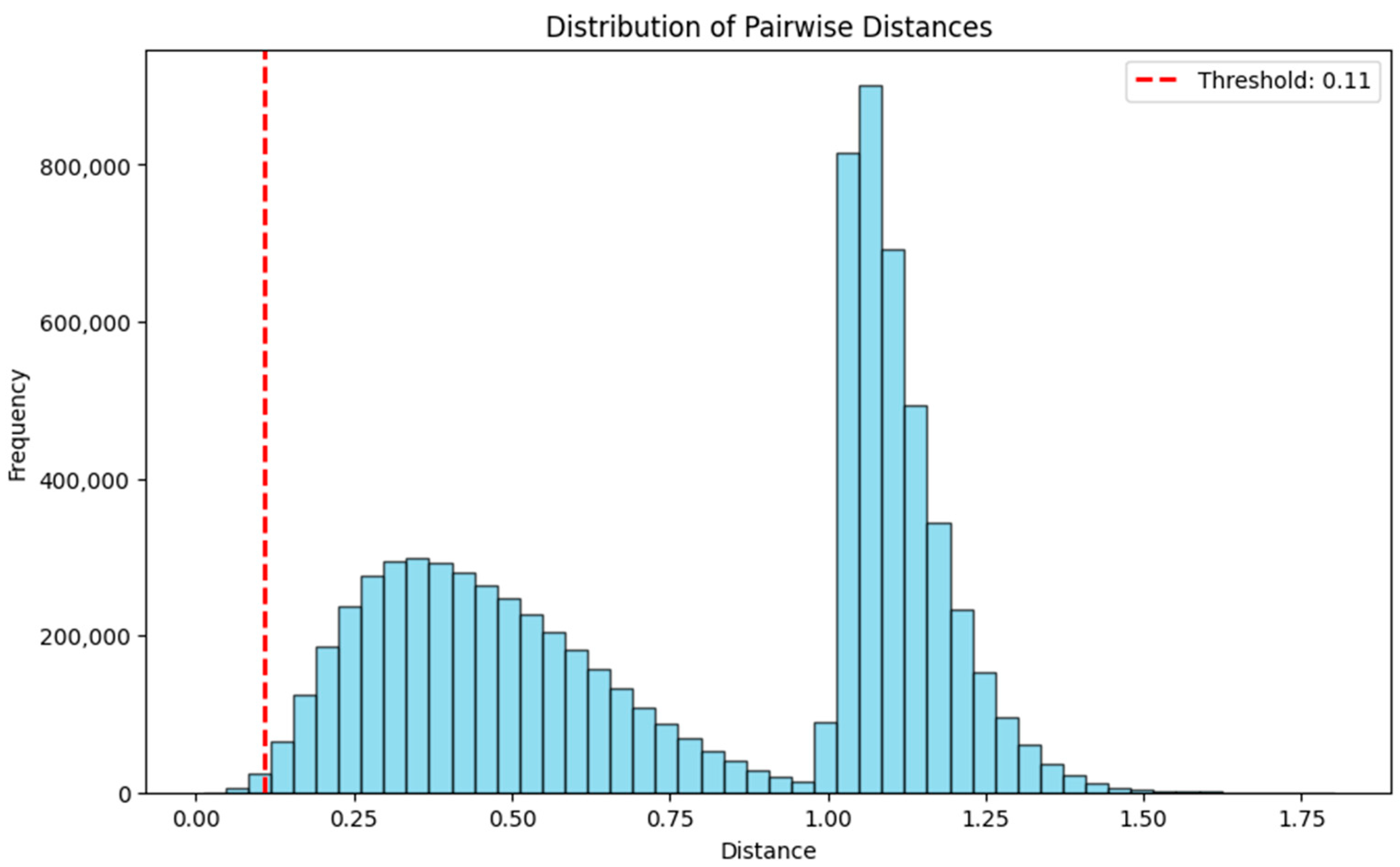
- Distance Calculation: The Euclidean distances from the new instance to all points in the training data are computed.
- Neighbor Identification: Points belonging to the same predicted class as the new instance are identified, and the number of these points within the defined distance threshold is calculated.
- Reliability Computation: Reliability is calculated as the total number of neighbors of the same class within the distance, divided by the “minimum cluster size” parameter. Reliability scores are capped at 1 for sufficiently dense regions.
3.3.4. ICM Method
- Neighbor Selection: The k-nearest neighbors of the new instance are identified from the training data using the Euclidean distance. These neighbors are then divided into two groups: representing neighbors that share the predicted label, and , representing neighbors with a label different from the predicted one.
- Sigma Calculation: is computed as the mean squared distance between the new instance x and its neighbors as shown inwhere N (x) is the set of all k-nearest neighbors.
- Weight Calculation: Each neighbor is assigned a weight based on its distance to the new instance, with the closer neighbors having greater influence. The weight of a neighbor is computed using
- Weighted Contributions for Support and Opposition: The average weighted contributions of the supporting () and opposing () neighbors are calculated as follows:where and denote the number of elements in and , respectively.
- Reliability Computation: The confidence score, C (x), is calculated as the difference between the weighted contributions of the supporting and opposing neighbors:
- The confidence score is then rescaled to the range [0, 1] using
3.3.5. Density and Local Fit Method
- Density Component: The density is computed by counting how many training data points fall within a predefined (Euclidean) distance threshold around the new instance. The count is limited to a maximum number of neighbors (“minimum cluster units”), ensuring that the density score is normalized to a range between 0 and 1.
- Data Agreement Component: The data agreement is calculated as the proportion of neighbors that share the same label as the predicted label of the new instance based on the distance threshold.
- ML Agreement Component: The ML agreement measures the consistency between the model’s predictions for the neighbors and the predicted label of the new instance (based on neighbors with consistent predictions divided by total neighbors within the threshold).
- Reliability Computation: The final reliability score is calculated by multiplying the three components. This formulation ensures that all three aspects contribute to reliability.
3.4. Parameter Selection for Methods
4. Experimental Results
4.1. Subtractive Clustering Method
4.2. DBSCAN Method
4.3. Distance-Based Method
4.4. ICM-Based Method
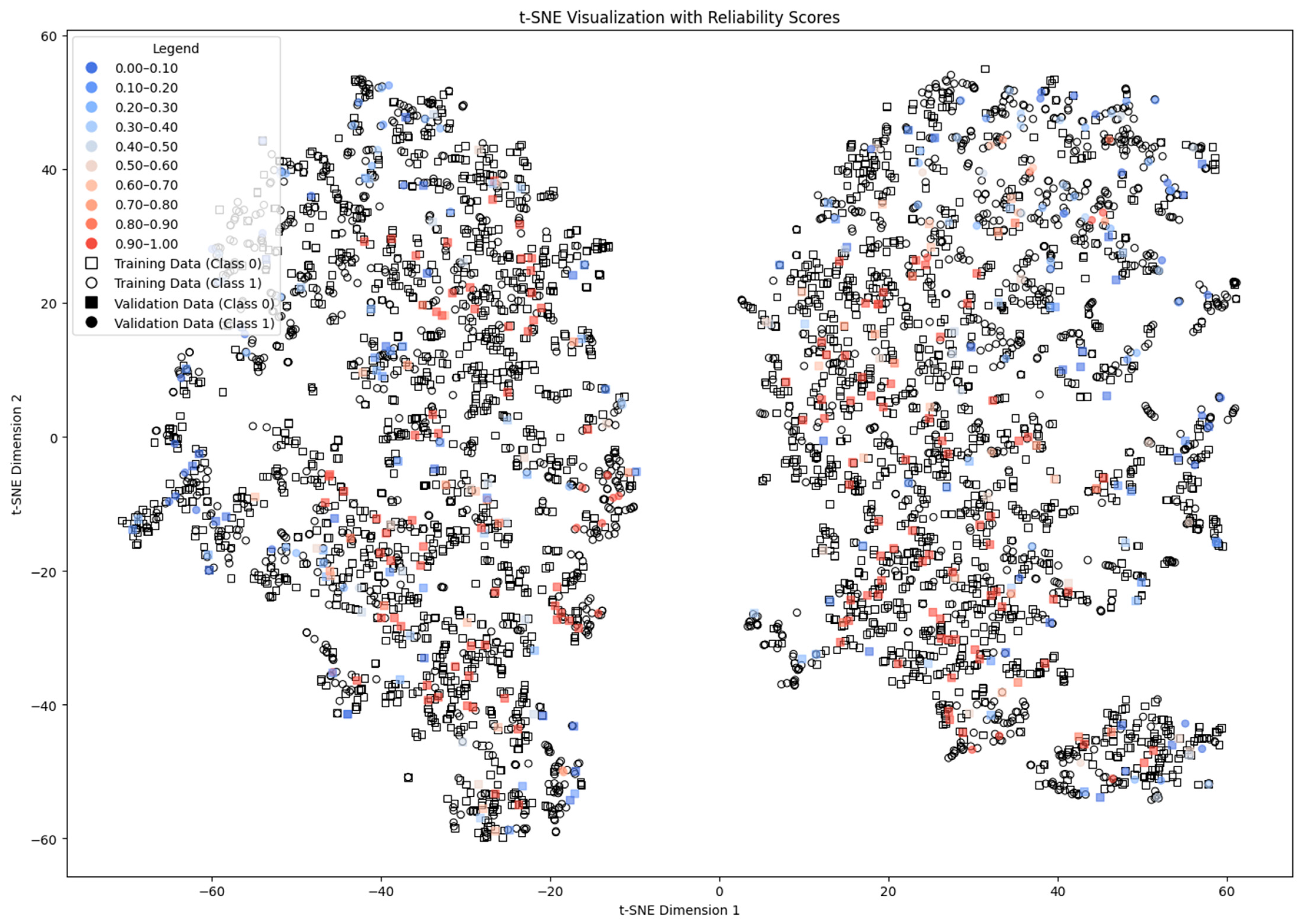
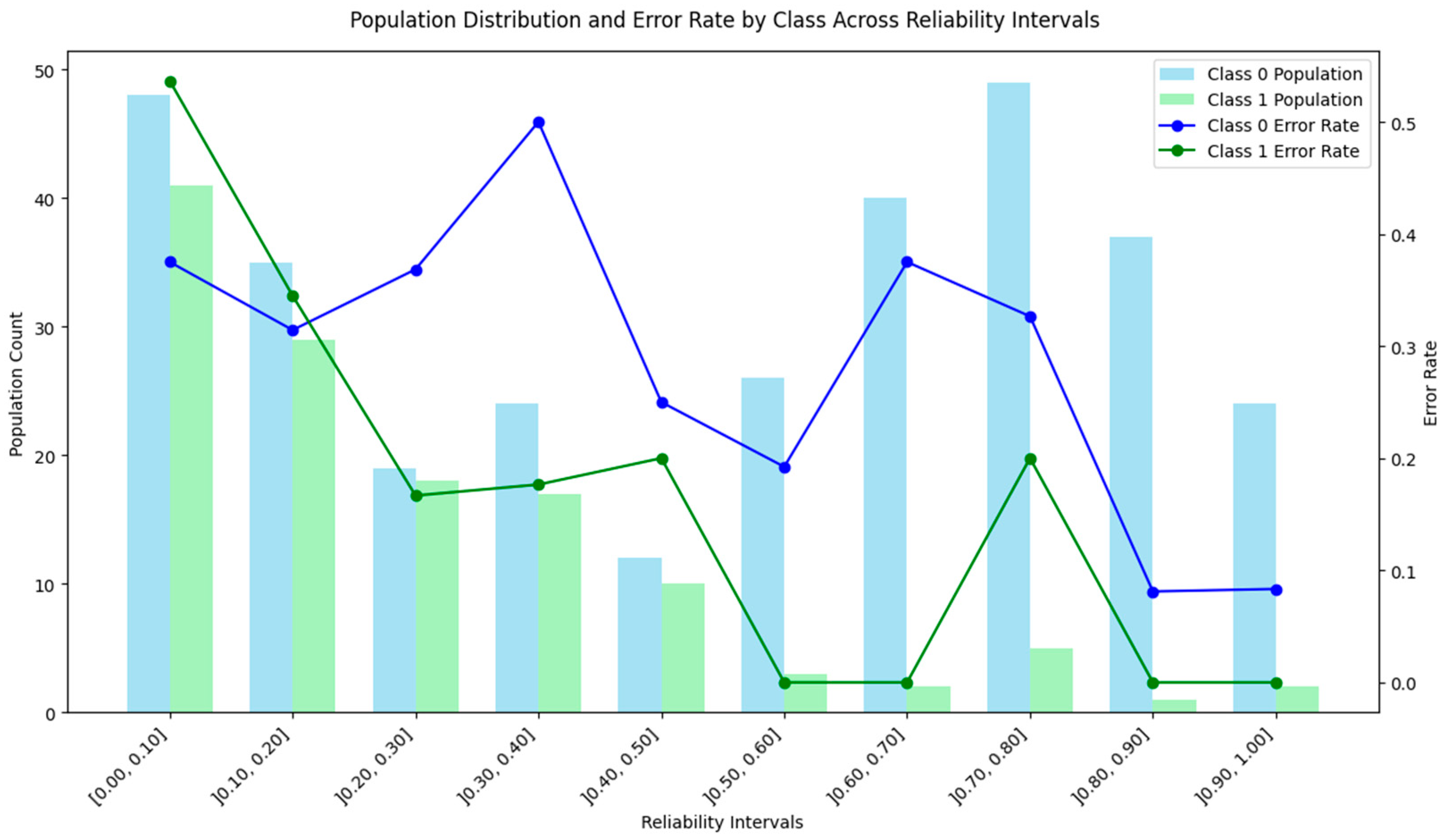
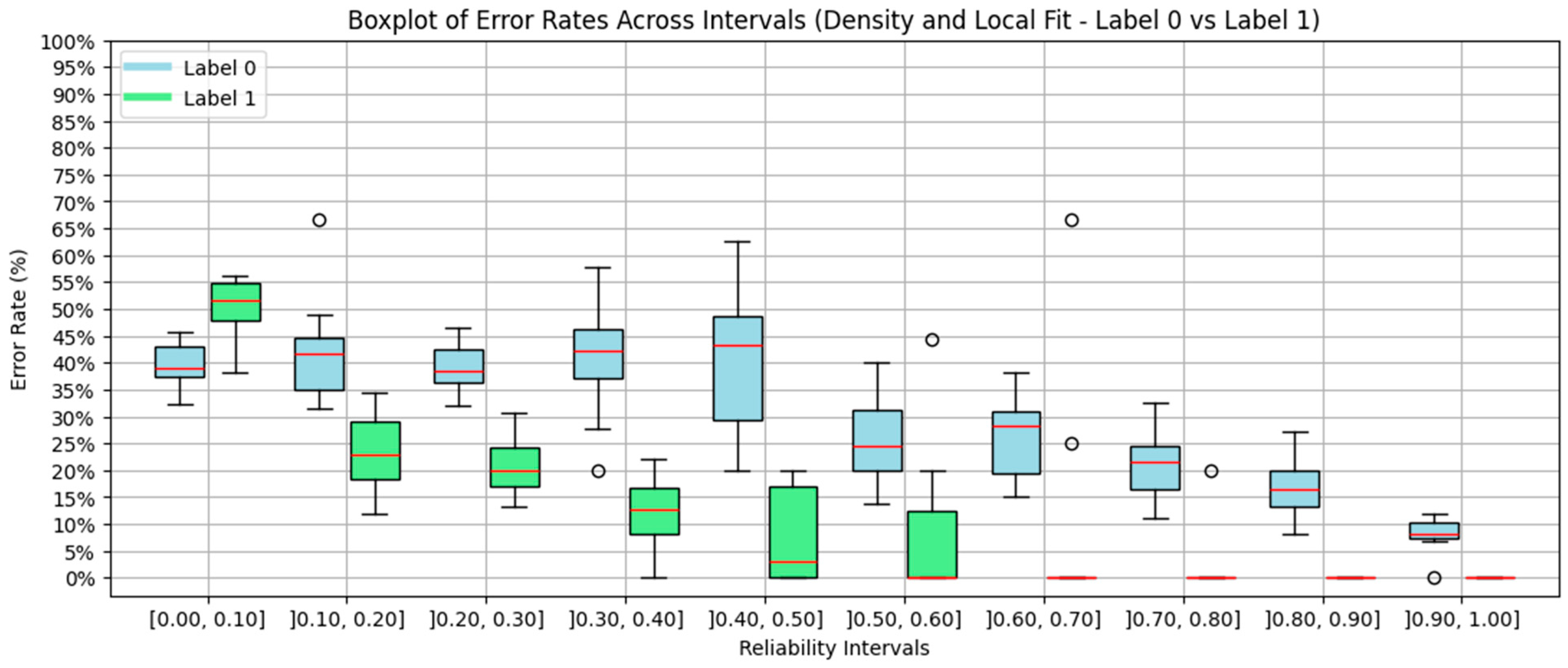
4.5. Density and Local Fit Combination Method
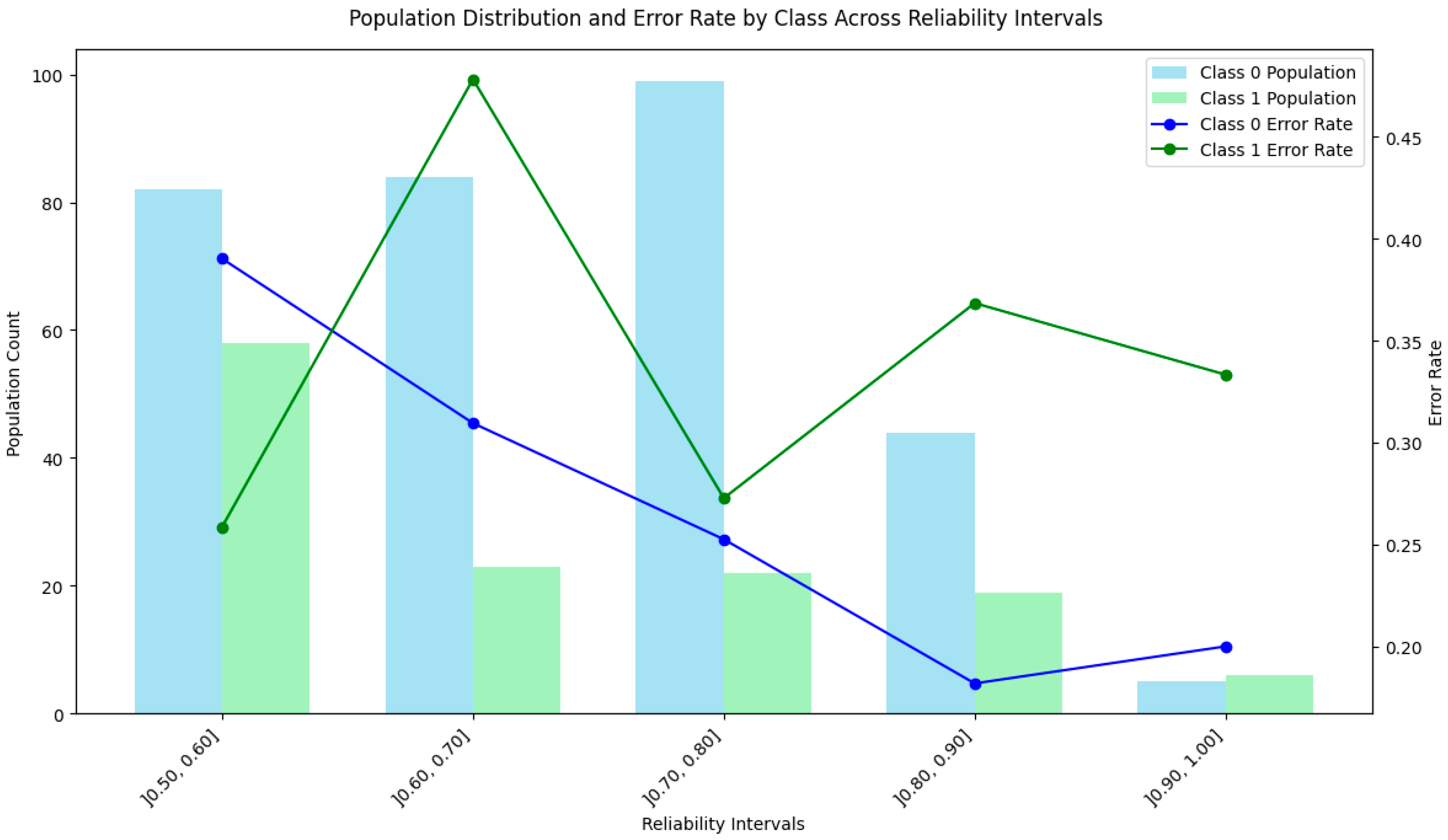
4.6. Aggregate Performance
4.7. Discussion of the Results
5. Conclusions and Future Work
Author Contributions
Funding
Institutional Review Board Statement
Informed Consent Statement
Data Availability Statement
Conflicts of Interest
Abbreviations
| DBSCAN | Density-Based Spatial Clustering of Applications with Noise |
| ICM | Interpretable confidence measure |
| ML | Machine learning |
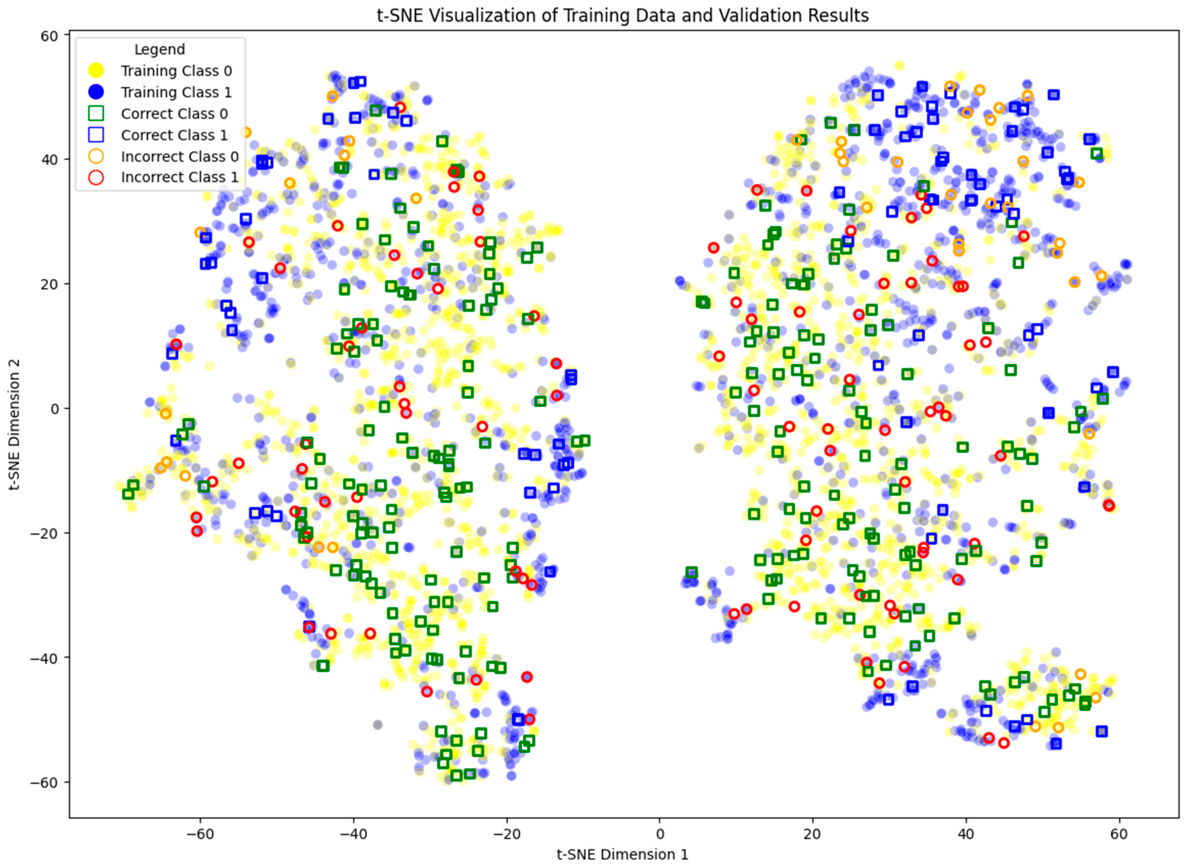
| t-SNE | t-distributed Stochastic Neighbor Embedding |
References
- Qayyum, A.; Qadir, J.; Bilal, M.; Al-Fuqaha, A. Secure and Robust Machine Learning for Healthcare: A Survey. IEEE Rev. Biomed. Eng. 2021, 14, 156–180. [Google Scholar] [CrossRef] [PubMed]
- Javaid, M.; Haleem, A.; Pratap Singh, R.; Suman, R.; Rab, S. Significance of Machine Learning in Healthcare: Features, Pillars and Applications. Int. J. Intell. Netw. 2022, 3, 58–73. [Google Scholar] [CrossRef]
- Schulam, P.; Saria, S. Can You Trust This Prediction? Auditing Pointwise Reliability after Learning. In Proceedings of the AISTATS 2019—22nd International Conference on Artificial Intelligence and Statistics, Okinawa, Japan, 16–18 April 2019. [Google Scholar]
- Nicora, G.; Rios, M.; Abu-Hanna, A.; Bellazzi, R. Evaluating Pointwise Reliability of Machine Learning Prediction. J. Biomed. Inform. 2022, 127, 103996. [Google Scholar] [CrossRef] [PubMed]
- Henriques, J.; Rocha, T.; Paredes, S.; Gil, P.; Loureiro, J.; Petrella, L. Pointwise Reliability of Machine Learning Models: Application to Cardiovascular Risk Assessment. In 9th European Medical and Biological Engineering Conference, Portorož, Slovenia, 9–13 June 2024; Jarm, T., Šmerc, R., Mahnič-Kalamiza, S., Eds.; Springer Nature: Cham, Switzerland, 2024; pp. 213–222. [Google Scholar]
- Saraygord Afshari, S.; Enayatollahi, F.; Xu, X.; Liang, X. Machine Learning-Based Methods in Structural Reliability Analysis: A Review. Reliab. Eng. Syst. Saf. 2022, 219, 108223. [Google Scholar] [CrossRef]
- Bud, M.A.; Moldovan, I.; Radu, L.; Nedelcu, M.; Figueiredo, E. Reliability of Probabilistic Numerical Data for Training Machine Learning Algorithms to Detect Damage in Bridges. Struct. Control Health Monit. 2022, 29, e2950. [Google Scholar] [CrossRef]
- van der Waa, J.; van Diggelen, J.; Neerincx, M.; Raaijmakers, S. ICM: An Intuitive Model Independent and Accurate Certainty Measure for Machine Learning. In 10th International Conference on Agents and Artificial Intelligence, Funchal, Portugal, 16–18 January 2018; SCITEPRESS—Science and Technology Publications: Setúbal, Portugal, 2018; pp. 314–321. [Google Scholar]
- van der Waa, J.; Schoonderwoerd, T.; van Diggelen, J.; Neerincx, M. Interpretable Confidence Measures for Decision Support Systems. Int. J. Hum. Comput. Stud. 2020, 144, 102493. [Google Scholar] [CrossRef]
- Hellman, M.E. The Nearest Neighbor Classification Rule with a Reject Option. IEEE Trans. Syst. Sci. Cybern. 1970, 6, 179–185. [Google Scholar] [CrossRef]
- Ester, M.; Kriegel, H.P.; Sander, J.; Xu, X. A Density-Based Algorithm for Discovering Clusters A Density-Based Algorithm for Discovering Clusters in Large Spatial Databases with Noise. In Proceedings of the Proceedings—2nd International Conference on Knowledge Discovery and Data Mining, KDD 1996, Portland, OR, USA, 2–4 August 1996. [Google Scholar]
- Nicora, G.; Bellazzi, R. A Reliable Machine Learning Approach Applied to Single-Cell Classification in Acute Myeloid Leukemia. AMIA Annu. Symp. Proc. 2021, 2020, 925. [Google Scholar] [PubMed]
- Kailkhura, B.; Gallagher, B.; Kim, S.; Hiszpanski, A.; Han, T.Y.J. Reliable and Explainable Machine-Learning Methods for Accelerated Material Discovery. NPJ Comput. Mater. 2019, 5, 108. [Google Scholar] [CrossRef]
- Bahrami, S.; Tuncel, E. An Efficient Running Quantile Estimation Technique alongside Correntropy for Outlier Rejection in Online Regression. In Proceedings of the 2020 IEEE International Symposium on Information Theory (ISIT), Los Angeles, CA, USA, 21–26 June 2020; IEEE: New York, NY, USA, 2020; pp. 2813–2818. [Google Scholar]
- Briesemeister, S.; Rahnenführer, J.; Kohlbacher, O. No Longer Confidential: Estimating the Confidence of Individual Regression Predictions. PLoS ONE 2012, 7, e48723. [Google Scholar] [CrossRef] [PubMed]
- Adomavicius, G.; Wang, Y. Improving Reliability Estimation for Individual Numeric Predictions: A Machine Learning Approach. INFORMS J. Comput. 2022, 34, 503–521. [Google Scholar] [CrossRef]
- Myers, P.D.; Ng, K.; Severson, K.; Kartoun, U.; Dai, W.; Huang, W.; Anderson, F.A.; Stultz, C.M. Identifying Unreliable Predictions in Clinical Risk Models. NPJ Digit. Med. 2020, 3, 8. [Google Scholar] [CrossRef] [PubMed]
- Valente, F.; Henriques, J.; Paredes, S.; Rocha, T.; de Carvalho, P.; Morais, J. A New Approach for Interpretability and Reliability in Clinical Risk Prediction: Acute Coronary Syndrome Scenario. Artif. Intell. Med. 2021, 117, 102113. [Google Scholar] [CrossRef] [PubMed]
- Correia, C. Pointwise-Benchmark. Available online: https://github.com/Oak10/pointwise-benchmark/releases/tag/1.1.1 (accessed on 17 April 2025).
- Cervati Neto, A.; Levada, A.L.M.; Ferreira Cardia Haddad, M. Supervised T-SNE for Metric Learning With Stochastic and Geodesic Distances. IEEE Can. J. Electr. Comput. Eng. 2024, 47, 199–205. [Google Scholar] [CrossRef]
- Li, K.; DeCost, B.; Choudhary, K.; Greenwood, M.; Hattrick-Simpers, J. A Critical Examination of Robustness and Generalizability of Machine Learning Prediction of Materials Properties. NPJ Comput. Mater. 2023, 9, 55. [Google Scholar] [CrossRef]
- Sadikin, M. EHR Dataset for Patient Treatment Classification. Mendeley Data 2020, 1, 2020. [Google Scholar]
- Chiu, S.L. Fuzzy Model Identification Based on Cluster Estimation. J. Intell. Fuzzy Syst. 1994, 2, 267–278. [Google Scholar] [CrossRef]
- Chandar, S.K. Stock Market Prediction Using Subtractive Clustering for a Neuro Fuzzy Hybrid Approach. Clust. Comput. 2019, 22, 13159–13166. [Google Scholar] [CrossRef]


| std) | Min | Max | Unique Values | |
|---|---|---|---|---|
| HAEMOGLOBINS | 3.8 | 18.9 | 126 | |
| ERYTHROCYTE | 1.4 | 7.8 | 425 | |
| LEUCOCYTE | 1.1 | 76.6 | 269 | |
| THROMBOCYTE | 10.0 | 1183.0 | 542 | |
| MCHC | 26.0 | 39.0 | 103 | |
| MCV | 54.0 | 115.6 | 401 | |
| AGE | 1 | 98.0 | 94 |
| Percentile | Distance Threshold | Minimum Cluster Unit |
|---|---|---|
| 0.1 | ~0.087 | 3 |
| 0.25 | ~0.107 | 9 |
| 0.5 | ~0.124 | 19 |
| 0.75 | ~0.136 | 29 |
| 5 | ~0.223 | 198 |
| Noise | Cluster 1 | Cluster 2 | Cluster 3 | Cluster 4 | Cluster 5 | |
|---|---|---|---|---|---|---|
| No.Instances | 2136 | 233 | 146 | 90 | 71 | 32 |
| Count Label 0 | 1291 | 202 | 109 | 68 | 55 | 15 |
| Count Label 1 | 845 | 31 | 37 | 22 | 16 | 17 |
| [0.0, 0.1] | ]0.1, 0.2] | ]0.2, 0.3] | ]0.3, 0.4] | ]0.4, 0.5] | ]0.5, 0.6] | ]0.6, 0.7] | ]0.7, 0.8] | ]0.8, 0.9] | ]0.9, 1.0] | |||
|---|---|---|---|---|---|---|---|---|---|---|---|---|
| Subtractive | Cases | Y = 0 | ||||||||||
| Y = 1 | ||||||||||||
| Error (%) | Y = 0 | |||||||||||
| Y = 1 | 0 | |||||||||||
| DBSCAN | Cases | Y = 0 | ||||||||||
| Y = 1 | ||||||||||||
| Error (%) | Y = 0 | |||||||||||
| Y = 1 | ||||||||||||
| Distance | Cases | Y = 0 | ||||||||||
| Y = 1 | ||||||||||||
| Error (%) | Y = 0 | |||||||||||
| Y = 1 | ||||||||||||
| ICM | Cases | Y = 0 | ||||||||||
| Y = 1 | ||||||||||||
| Error (%) | Y = 0 | |||||||||||
| Y = 1 | 2 | |||||||||||
| D. Local | Cases | Y = 0 | ||||||||||
| Y = 1 | ||||||||||||
| Error (%) | Y = 0 | |||||||||||
| Y = 1 |
Disclaimer/Publisher’s Note: The statements, opinions and data contained in all publications are solely those of the individual author(s) and contributor(s) and not of MDPI and/or the editor(s). MDPI and/or the editor(s) disclaim responsibility for any injury to people or property resulting from any ideas, methods, instructions or products referred to in the content. |
© 2025 by the authors. Licensee MDPI, Basel, Switzerland. This article is an open access article distributed under the terms and conditions of the Creative Commons Attribution (CC BY) license (https://creativecommons.org/licenses/by/4.0/).
Share and Cite
Correia, C.; Paredes, S.; Rocha, T.; Henriques, J.; Bernardino, J. Benchmarking Methods for Pointwise Reliability. Information 2025, 16, 327. https://doi.org/10.3390/info16040327
Correia C, Paredes S, Rocha T, Henriques J, Bernardino J. Benchmarking Methods for Pointwise Reliability. Information. 2025; 16(4):327. https://doi.org/10.3390/info16040327
Chicago/Turabian StyleCorreia, Cláudio, Simão Paredes, Teresa Rocha, Jorge Henriques, and Jorge Bernardino. 2025. "Benchmarking Methods for Pointwise Reliability" Information 16, no. 4: 327. https://doi.org/10.3390/info16040327
APA StyleCorreia, C., Paredes, S., Rocha, T., Henriques, J., & Bernardino, J. (2025). Benchmarking Methods for Pointwise Reliability. Information, 16(4), 327. https://doi.org/10.3390/info16040327