Stroke Detection in Brain CT Images Using Convolutional Neural Networks: Model Development, Optimization and Interpretability

Abstract

Stroke detection using medical imaging plays a crucial role in early diagnosis and treatment planning. In this study, we propose a Convolutional Neural Network (CNN)-based model for detecting strokes from brain Computed Tomography (CT) images. The model is trained on a dataset consisting of 2501 images, including both normal and stroke cases, and employs a series of preprocessing steps, including resizing, normalization, data augmentation, and splitting into training, validation, and test sets. The CNN architecture comprises three convolutional blocks followed by dense layers optimized through hyperparameter tuning to maximize performance. Our model achieved a validation accuracy of 97.2%, with precision and recall values of 96%, demonstrating high efficacy in stroke classification. Additionally, interpretability techniques such as Local Interpretable Model-agnostic Explanations (LIME), occlusion sensitivity, and saliency maps were used to visualize the model’s decision-making process, enhancing transparency and trust for clinical use. The results suggest that deep learning models, particularly CNNs, can provide valuable support for medical professionals in detecting strokes, offering both high performance and interpretability. The model demonstrates moderate generalizability, achieving 89.73% accuracy on an external, patient-independent dataset of 9900 CT images, underscoring the need for further optimization in diverse clinical settings.

1. Introduction

Stroke is a severe health condition caused by disrupted blood supply to the brain, leading to oxygen/nutrient deprivation and cell damage. It is a leading cause of mortality and long-term disability worldwide, affecting millions annually. Around 800,000 new or recurrent strokes occur yearly, with 87% ischemic, 10% intracranial hemorrhagic, and 3% subarachnoid hemorrhagic [1]. While stroke incidence has declined in high-income countries (HICs) over the past three decades, projections estimate 3.4 million additional cases in the US by 2030 [2]. Advanced therapies like endovascular thrombectomy (EVT) and thrombolytics have improved outcomes, yet disparities persist. Reperfusion therapies (e.g., EVT) are predominantly available in HICs, with no low-income countries offering EVT [3]. These inequities highlight the urgent need for scalable diagnostic tools.

CT imaging is the gold standard for stroke diagnosis in emergency settings due to its speed and ability to differentiate stroke types. However, interpretation relies on radiologist expertise, which is time-consuming and prone to variability. The integration of artificial intelligence (AI), particularly Convolutional Neural Networks (CNNs), offers a promising solution. CNNs excel in image recognition by learning spatial hierarchies from data, requiring minimal manual feature engineering [4]. Their success in medical imaging (e.g., Magnetic Resonance Imaging (MRI) analysis) underscores their potential for stroke detection [5].

Despite advancements in imaging, timely and accurate stroke diagnosis remains challenging due to human error, workload pressures, and geographic disparities in care. Traditional methods lack scalability and global access to specialists is limited. AI-driven automation could address these gaps, yet existing CNN models for stroke detection often lack interpretability and validation in real-world settings. Bridging this gap requires robust, transparent models validated for clinical use.

This study aims to:

• Develop a CNN model tailored for stroke detection in CT images.
• Evaluate performance using metrics like accuracy, precision, recall, F1-score, and area under the receiver operating characteristic curve (AUC-ROC).
• Enhance interpretability via explainability techniques to build clinical trust.
• Optimize the model through hyperparameter tuning for maximal efficiency.

This study contributes three key advancements:

• A computationally efficient model (20.1 M parameters, 76.79 MB memory) tailored for real-time stroke detection, outperforming hybrid models like in memory efficiency.
• The first-of-its-kind application of LIME, occlusion sensitivity, and saliency maps to explain stroke predictions in CT imaging.
• Rigorous testing on 9900 images from multi-center sources, addressing a critical gap in prior works.

While prior studies have achieved high accuracy in stroke detection, this study focuses on balancing performance with computational efficiency to ensure real-time applicability in clinical settings. By developing a CNN model that balances both high accuracy and computational efficiency, this study is validated on both a training dataset of 2501 images and an external dataset of 9900 images. The model achieves a validation accuracy of 97.2% and recall of 96%, demonstrating its ability to maintain high performance while significantly reducing computational complexity.

This work advances stroke care by proposing an AI tool that enhances diagnostic speed and accuracy, particularly in resource-limited settings. By prioritizing transparency, the model supports clinician decision-making, aligning with global efforts to reduce disparities in stroke management [6]. The model was further validated on an expanded external dataset of 9900 CT images collected from multi-center sources. While performance on this dataset (89.73% accuracy) reflects room for improvement in heterogeneous environments, it confirms feasibility for real-world deployment with targeted refinements. While pre-trained CNNs offer advantages in feature extraction, this study opts for an end-to-end trained CNN to ensure domain-specific feature learning, particularly given the availability of a sufficiently large dataset. Additionally, this study emphasizes the importance of hyperparameter tuning and model interpretability, both of which are crucial for developing robust and clinically applicable deep-learning models.

The remainder of this article is organized as follows. Following this introduction, Section 2 provides a comprehensive review of prior research on AI and machine learning applications for stroke detection, highlighting key advancements and gaps in existing approaches. Section 3 outlines the methodology of the current study, detailing the data preprocessing pipeline, CNN model architecture, training procedures, and evaluation metrics used to assess performance. Section 4 presents the results, including quantitative metrics (e.g., accuracy, precision, recall) and qualitative insights from interpretability analyses. Section 5 discusses the findings, contextualizing the results within existing literature, addressing limitations, and exploring implications for clinical practice and future research. Finally, Section 6 concludes the article by summarizing the study’s contributions and proposing directions for further investigation.

2. Related Works

Ischemic stroke, which results from the blockage of blood flow to the brain, is a major health concern worldwide, responsible for a significant number of fatalities and long-term disabilities. The UK, for example, reports a stroke every five minutes, with over 100,000 cases annually and over 1.3 million stroke survivors as of 2023 [7]. The early detection of ischemic stroke plays a crucial role in determining treatment effectiveness and improving patient outcomes. Non-Contrast Computed Tomography (NCCT) has become the standard imaging modality for initial stroke diagnosis due to its availability, speed, and cost-effectiveness. However, NCCT often faces challenges in detecting ischemic strokes, particularly in the hyper-acute phase, due to subtle changes in brain tissue density.

Recent advances in deep learning (DL) technologies, particularly CNNs, have shown considerable promise in addressing these challenges. By enabling more accurate and automated analysis of NCCT images, DL models have the potential to enhance stroke diagnosis and facilitate early intervention. As research in this area progresses, it is essential to examine the current landscape of deep learning approaches for stroke detection and segmentation, including the performance of different models, their clinical applicability, and the gaps that remain in the field.

2.1. Deep Learning Approaches for Stroke Detection

2.1.1. Single-Stage Models

Several studies have focused on single-stage deep learning models for stroke detection, often utilizing CNN architecture. For instance, ref. [8] employed the ResNet50 architecture to classify slices of NCCT images, achieving an accuracy of 87.2% in slice classification. Similarly, ref. [9] introduced a symmetry-sensitive CNN that leverages hemisphere symmetry for stroke detection, providing a novel approach to identifying strokes (see

Table 1. Performance Metrics of Single-Stage Deep Learning Models for Stroke Detection.

Study	Architecture	Dataset Size	Accuracy	Key Contribution
[8]	ResNet50	130+	87.20% (slice)	Pre-trained models for slice classification and tissue segmentation.
[9]	Symmetry-sensitive CNN	217	90.1%	Novel model leveraging hemisphere symmetry for stroke detection.

for performance metrics).

2.1.2. Multi-Stage Models

Multi-stage models have gained attention for their ability to combine different CNN architectures to enhance performance. For example, ref. [10] developed a two-stage model integrating U-Net and ResNet, enabling the model to process both global and local information. This approach achieved an accuracy range of 85.7% to 91.9%. Another notable approach by [11] utilized a hybrid CNN architecture combining C-Net and INet, reaching an impressive accuracy of 99.54%. This demonstrated the effectiveness of integrating multiple network types (see

Table 2. Performance Metrics of Multi-Stage Deep Learning Models for Stroke Detection.

Study	Architecture	Dataset Size	Accuracy	Key Contribution
[10]	Two-stage CNN (U-Net + ResNet)	277	85.71–91.89%	Cascaded structure combining global and local information for stroke detection.
[11]	Hybrid CNN (C-Net + INet)	6650	99.54%	Combining C-Net and INet architectures for improved accuracy.

for performance metrics). While study [11] reports exceptional accuracy (99.54%) and recall (99.66%) using its hybrid CNN architecture (C-Net + INet), its computational complexity (26.8 M parameters, 321.6 MB training memory) limits real-world deployment. In contrast, our model achieves a balanced trade-off between performance (97.2% accuracy, 96% recall) and efficiency (20.1 M parameters, 76.79 MB memory), reducing computational costs by 25% (parameters) and 76% (memory) while maintaining clinical utility. This streamlined architecture prioritizes deployability in resource-constrained settings without relying on multi-stage networks.

2.2. Model Optimization and Interpretability

Optimization and interpretability are key considerations in the development of deep learning models for clinical use. Ref. [12] incorporated the Convolutional Block Attention Module (CBAM) into the ResNet architecture, resulting in improved attention to relevant features, achieving an accuracy of 95%. In another study, ref. [13] introduced a 3D CNN (nnUNet) for ischemic core segmentation, achieving a Dice coefficient of 0.46–0.47, comparable to expert radiologists. These studies highlight the importance of optimizing models for both performance and interpretability in clinical applications (see

Table 3. Performance Metrics of Optimized Deep Learning Models for Stroke Detection and Segmentation.

Study	Architecture Modification	Dataset Size	Accuracy	Key Contribution
[12]	ResNet-CBAM	2501	95%	Incorporating CBAM for improved feature attention in stroke detection.
[13]	3D CNN (nnUNet)	232	0.46–0.47 (Dice)	Optimized model for ischemic core segmentation comparable to expert radiologists.

for performance metrics).

2.3. Clinical Integration and Validation

For deep learning models to be integrated into clinical practice, they must be validated in real-world, multi-center settings. The authors of [10] conducted multi-center experiments and demonstrated the robustness of their two-stage CNN model across different datasets. Similarly, ref. [13] validated their 3D CNN model and demonstrated its non-inferiority compared to expert radiologists in ischemic core segmentation, making a significant step toward clinical acceptance (see

Table 4. Performance Metrics of Deep Learning Models in Multi-Center Validation and Clinical Settings.

Study	Multi-Center Validation	Control Group	Key Contribution
[10]	Yes	Yes	Multi-center experiments demonstrating robustness across different datasets.
[13]	Yes	Yes	Non-inferiority of DL model compared to expert radiologists in segmentation.

for performance metrics).

2.4. GAP Analysis

Despite advancements in deep learning models for stroke detection, several gaps remain that align closely with the aims and objectives of this study. These gaps include the following:

• Data Limitations: Many existing models rely on relatively small and often homogeneous datasets, which can hinder their ability to generalize across diverse populations and clinical settings [14]. This study addresses data limitations by incorporating a larger and more diverse dataset (2501 images for training/validation and 9900 images for testing), enhancing the model’s capacity to generalize across different stroke types and imaging qualities. By expanding the dataset, this study aims to improve the model’s generalizability, which is crucial for ensuring accurate stroke detection across a variety of clinical environments and imaging conditions.
• While related studies [11,12] utilized datasets of 6650 and 2501 images, respectively, this study enhances generalizability through external validation on 9900 CT images from diverse institutions. Though the training dataset (2501 images) is smaller, the external validation set is 10x larger than [11], which ensures robustness across heterogeneous imaging protocols and stroke subtypes. This approach addresses a key gap in prior works, such as overreliance on single-center data.
• Model Complexity and Efficiency: High computational costs can limit the practical use of complex models such as ResNet50 in real-time clinical settings [15]. This study aims to optimize the CNN architecture through hyperparameter tuning to achieve maximal efficiency, reducing computational complexity while maintaining accuracy for real-time stroke detection. The proposed model reduces computational complexity through optimized architecture design, achieving high performance with significantly fewer operations compared to more complex models such as in [11]. While the model’s external accuracy (89.73%) trails state-of-the-art benchmarks, its streamlined architecture (20 M parameters) ensures practicality for real-time use, addressing a key clinical need. These optimizations enable real-time inference on standard clinical hardware, addressing a critical barrier to AI adoption in stroke care.
• Segmentation and Localization: While stroke detection accuracy is improving, the precise segmentation and localization of ischemic lesions remain a challenge [16]. Accurate segmentation of the ischemic core is crucial for guiding clinical decision-making. This study will focus on developing a CNN-based model tailored for stroke detection in CT images, with the goal of achieving high accuracy in ischemic stroke localization.
• Interpretability and Clinical Trust: Many deep learning models lack transparency, limiting their acceptance in clinical practice [17]. This study will enhance the interpretability of the CNN model using explainability techniques, thereby building clinical trust by providing clear visual explanations for stroke predictions.
• Real-World Validation: Although existing models have shown potential in controlled settings, their validation in real-world clinical environments is often limited [18]. This study aims to evaluate the performance of the CNN model using key metrics such as accuracy, precision, recall, F1-score, and AUC-ROC, ensuring its reliability and effectiveness for real-world clinical use.

Deep learning, particularly CNNs, holds substantial promise for improving ischemic stroke detection and segmentation, especially in NCCT images. However, several challenges remain, including the need for larger datasets, more efficient models, improved segmentation accuracy, better interpretability, and real-world validation. Addressing these challenges will ensure that deep learning models can be effectively integrated into clinical practice, improving stroke diagnosis and patient outcomes. This study, with its focus on developing a tailored CNN model, optimizing its performance, improving interpretability, and evaluating its clinical applicability, directly addresses these gaps and contributes to advancing AI-driven stroke diagnosis.

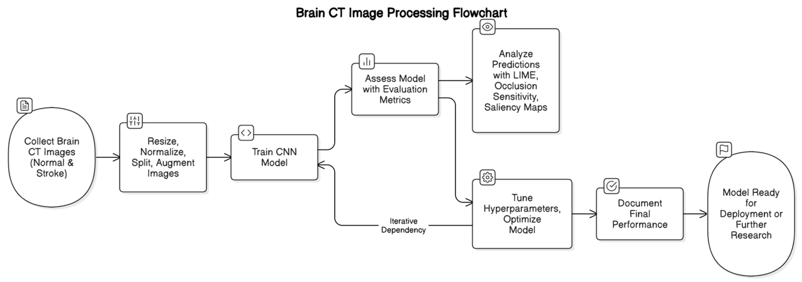
3. Materials and Methods

This section outlines the systematic approach employed to develop and validate a CNN model for the detection of brain strokes using CT images. The methodology encompasses multiple stages, as illustrated in Figure 1.

First, a dataset of brain CT images, consisting of both normal and stroke cases, is collected. The images then undergo preprocessing steps, including resizing, normalization, splitting into training and validation sets, and augmentation to enhance model generalization.

Following preprocessing, a CNN model is trained on the processed dataset. Model performance is assessed using evaluation metrics, and interpretability techniques such as LIME, occlusion sensitivity, and saliency maps are employed to analyze predictions. Based on these analyses, hyperparameter tuning and optimization are conducted iteratively to enhance model accuracy and robustness.

Once an optimal model is achieved, final performance metrics are documented. The model is then prepared for deployment in a clinical setting or further research, as depicted in Figure 1.

3.1. Data Collection and Preprocessing

3.1.1. Dataset Description

The dataset utilized in this study consists of two categories of brain CT images: “Normal” and “Stroke”. The dataset comprises a total of 2501 images, with 1551 Normal and 950 Stroke images, each varying in size and resolution. The “Stroke” category includes images depicting cerebral hemorrhages or ischemic regions, whereas the “Normal” category represents healthy brain anatomy. More details about the dataset can be found at https://www.kaggle.com/datasets/afridirahman/brain-stroke-ct-image-dataset (accessed on 14 December 2024).

3.1.2. Preprocessing Pipeline

To ensure consistency and compatibility with the model input requirements, the following preprocessing steps were applied:

• Image Resizing: All images were resized to a uniform dimension of 256 × 256 pixels using bilinear interpolation [19]. This standardization ensures consistency across all samples while preserving critical anatomical features, which is crucial for accurate stroke detection by the CNN.
• Normalization: Pixel values were normalized to the range [0, 1] by dividing by 255 [20]. This normalization step accelerates the convergence of the model during training by scaling the input features to a standard range.

  $$I_{normalized}={\displaystyle \frac{I_{original}}{255}}$$
• Data Splitting: The dataset was partitioned into three subsets: training (80%), validation (10%), and testing (10%). This split ensures that the model is trained on a substantial portion of the data, while separate validation and test sets provide unbiased evaluations of its performance [21].
• Data Augmentation: To enhance the model’s generalization capabilities and mitigate overfitting, data augmentation techniques were applied to the training set. These techniques included rotation, width and height shifts, shear, zoom, and horizontal flipping. By introducing variability in the training data, the model becomes more robust to unseen data.

  o

  Rotation: For an angle θ, the rotation matrix is

  $$R\left(\theta \right)=\left[\begin{array}{cc}\cos \left(\theta \right)& -\sin \left(\theta \right)\\ \sin \left(\theta \right)& \cos \left(\theta \right)\end{array}\right]$$

  o

  Translation (Shifting): For a shift in the x and y directions by δ_x and δ_y, respectively:

  $$T\left({\delta }_x,{\delta }_y\right)=\begin{array}{ccc}1& 0& {\delta }_x\\ 0& 1& {\delta }_y\\ 0& 0& 1\end{array}$$

  o

  Scaling (Zooming): To scale an image by a factor s, the scaling matrix is:

  $$S\left(s\right)=\left[\begin{array}{cc}s& 0\\ 0& s\end{array}\right]$$

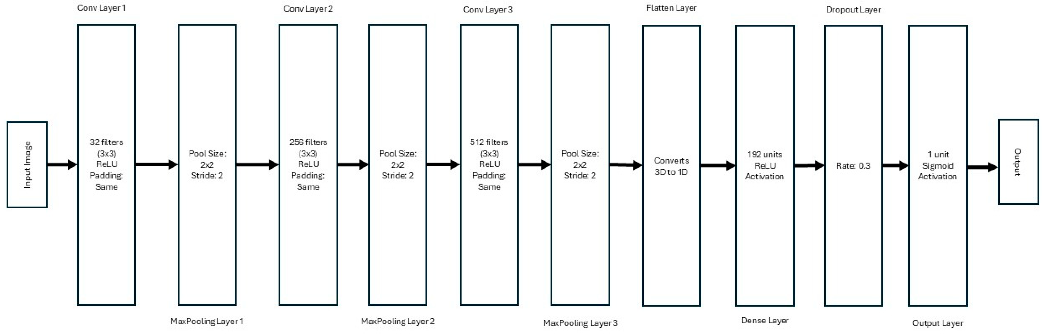
3.2. Model Development

3.2.1. Architecture Design

The CNN architecture was designed to extract hierarchical features from the preprocessed CT images. The model comprises three convolutional blocks followed by dense layers for classification, as shown in Figure 2.

• Convolutional Blocks:

  o

  First Block: 32 filters with a kernel size of 3 × 3, using the ReLU activation function and ‘same’ padding, followed by a 2 × 2 max-pooling layer.

  o

  Second Block: 256 filters with a kernel size of 3 × 3, ReLU activation, and ‘same’ padding, followed by a 2 × 2 max-pooling layer.

  o

  Third Block: 512 filters with a kernel size of 3 × 3, ReLU activation, and ‘same’ padding, followed by a 2 × 2 max-pooling layer.

• Dense Layers: A flattened layer converts the 3D output of the convolutional layers into a 1D vector. This is followed by a dense layer with 192 units and ReLU activation. A dropout layer with a rate of 0.3 is included to prevent overfitting.
• Output Layer: The final layer consists of a single neuron with sigmoid activation, enabling binary classification for stroke detection.

3.2.2. Hyperparameter Optimization and Fine-Tuning

To enhance the model’s performance and identify the optimal hyperparameter configuration, a systematic optimization process was implemented using the Keras Tuner framework. This approach leverages automated hyperparameter search to explore the hyperparameter space and maximize validation accuracy.

The hyperparameter optimization process was designed to explore a predefined search space, which included critical architectural and training parameters. The search space comprised the following hyperparameters:

• Convolutional Layer Filters: The number of filters in each convolutional layer was varied to explore different levels of feature extraction granularity. The search range included values of 32, 64, 96, 128, 160, 192, 224, and 256 filters for the first, second, and third convolutional layers, respectively. This parameter directly influences the model’s capacity to learn hierarchical features from the input images.
• Learning Rate: The learning rate of the Adam optimizer was tuned to ensure efficient convergence during training. The search space included values of 0.0001, 0.0005, and 0.001. An appropriate learning rate balances the speed of convergence and the stability of the training process.
• Dropout Rate: To mitigate overfitting, the dropout rate in the dense layers was optimized. The search range included values of 0.2, 0.3, 0.4, and 0.5. Dropout randomly deactivates a fraction of neurons during training, forcing the network to learn redundant representations and improving generalization.
• Dense Layer Units: The number of units in the dense layer was varied to explore different levels of model complexity. The search range included values of 64, 128, 192, and 256 units. This parameter affects the model’s ability to learn complex mappings from features to output predictions.

The Keras Tuner’s RandomSearch algorithm was employed to conduct a comprehensive search over the defined hyperparameter space. This algorithm randomly samples candidate configurations from the search space and evaluates their performance based on validation accuracy. A total of 100 trials were conducted, each evaluating a unique combination of hyperparameters.

The optimization process was integrated with 5-fold cross-validation, where the dataset was partitioned into five folds. Each fold served as the validation set once, while the remaining data were used for training. This ensured unbiased evaluation and robustness across different data subsets.

Data augmentation techniques, such as rotation (±15°), width and height shifts (±10%), shear (±0.1), zoom (±0.1), and horizontal flipping, were applied to the training set to improve generalization and reduce overfitting.

The model was trained using the Adam optimizer with the learning rate specified by the hyperparameter search. Binary cross-entropy loss was used as the loss function, and the model was compiled to optimize for accuracy. Training was conducted for 15 epochs, with a batch size of 8. To prevent overfitting, early stopping was implemented with a patience of 5 epochs. If the validation loss did not improve for five consecutive epochs, training was halted, and the best weights were restored.

Following the completion of 100 trials, the hyperparameter configuration with the highest validation accuracy was identified. The optimal configuration consisted of the following hyperparameters:

• Convolutional Filters: 32 (Layer 1), 256 (Layer 2), 512 (Layer 3);
• Learning Rate: 0.0005;
• Dropout Rate: 0.3;
• Dense Units: 192.

Using this configuration, the model achieved a validation accuracy of 97.2%. The best-performing model was saved for further evaluation and potential deployment.

3.2.3. Training Procedure

The model was trained using the Adam optimizer, which uses the following update rule for each parameter θ iteration t:

$${\theta }_{t+1}={\theta }_t-\alpha .{\displaystyle \frac{m_t}{\sqrt{v_t+\in }}}$$

where

• α is the learning rate;
• m_t is the first moment estimate (mean of gradients);
• v_t is the second moment estimate (variance of gradients);
• ϵ is a small constant to prevent division by zero.

3.2.4. Baseline Models

To evaluate the performance of the proposed CNN model, several well-established architectures were used as baseline models. These models are commonly applied to image classification tasks and represent a range of architectures with varying depths and complexities. To benchmark performance, the established architectures used for the study, Xception, ResNet50, AlexNet, and VGG16, were trained on the same dataset using identical preprocessing and evaluation protocols.

• Xception: It is an extension of the Inception architecture, introducing depthwise separable convolutions. This allows for more efficient processing, reducing the number of parameters while maintaining high accuracy. The architecture consists of 36 convolutional layers, and it has been shown to perform exceptionally well in image classification tasks. We trained the Xception model with the same dataset, preprocessing steps, and training procedure as the proposed CNN.
• ResNet50: It is a deep residual network that includes 50 layers and employs residual connections to address the vanishing gradient problem during training. The key advantage of ResNet50 is its ability to train deeper networks effectively, preserving information across many layers. This model was selected as a benchmark due to its widespread use in a variety of image recognition tasks and its demonstrated capability to achieve high accuracy in medical image classification.
• AlexNet: It is one of the earliest deep CNN architectures and is known for its breakthrough performance in the 2012 ImageNet competition. It consists of eight layers, including five convolutional layers and three fully connected layers. Although older compared to the other models in this study, AlexNet remains a significant baseline for medical imaging tasks due to its simplicity and historical importance in CNN development.
• VGG16: It is known for its simplicity and depth and has 16 layers (13 convolutional layers and 3 fully connected layers). The VGG architecture is characterized by its use of small 3 × 3 filters and a relatively uniform architecture, which allows for deeper networks. VGG16 has been a staple in the computer vision community and serves as a reliable benchmark for comparing more complex architectures.

3.3. Model Evaluation

To assess the performance of each model, we used the same evaluation metrics as the proposed model, including accuracy, precision, recall, F1-score, and AUC-ROC. Additionally, we performed a cross-validation procedure to ensure robust performance across different folds of the data. The results of the baseline models were compared to the proposed CNN model, with a focus on accuracy, computational efficiency, and generalizability.

3.3.1. Evaluation Metrics

The model’s performance was evaluated using accuracy, precision, recall, F1-score, and AUC-ROC. These metrics provide a comprehensive assessment of the model’s classification capabilities.

3.3.2. Validation Strategy

To ensure robust evaluation, the dataset was partitioned into training (80%), validation (10%), and test (10%) sets. The reported validation accuracy of 97.2% corresponds to a single hold-out validation split used during hyperparameter optimization. To further strengthen validation rigor, we implemented stratified 5-fold cross-validation, ensuring a balanced representation of stroke and normal cases in each fold. This approach mitigates biases from class imbalance (1551 normal vs. 950 stroke images) and provides a more generalized performance estimate.

• Cross-Validation: 5-fold cross-validation was implemented to ensure robustness. The dataset was partitioned into five folds, with each fold serving as the validation set once while the remaining data were used for training.
• Test Set Assessment: The final model was evaluated on an unseen test set to estimate real-world performance. The test set comprised 200 images (10% of the dataset).
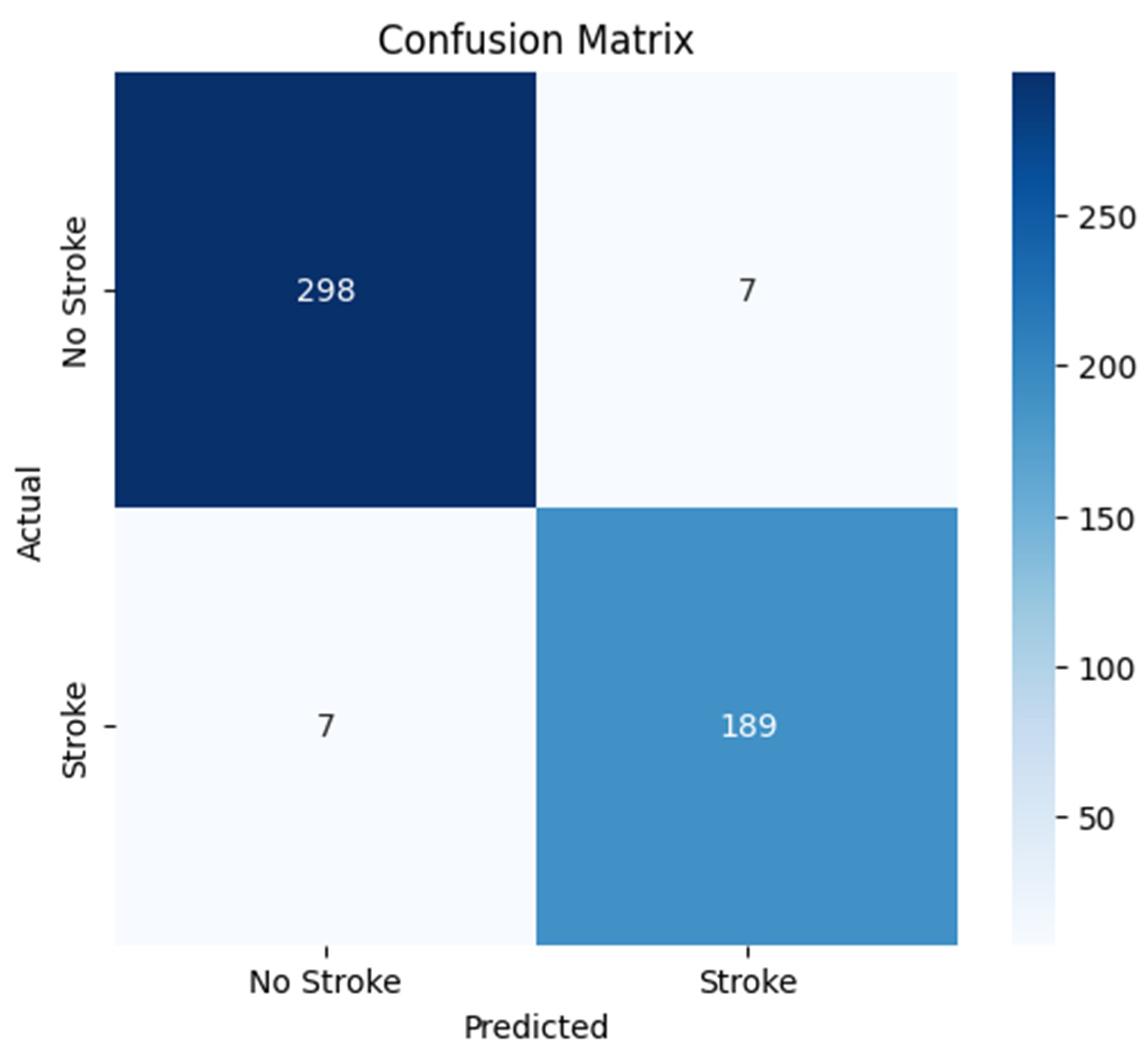
• Confusion Matrix: A confusion matrix was generated to analyze class-specific performance, providing insights into the model’s ability to correctly classify “Stroke” and “Normal” images.

3.3.3. Quantitative Performance Metrics

The model achieved a validation accuracy of 97.2%, with a precision of 96% and recall of 96% for the “Stroke” class. The AUC-ROC score was 0.98, indicating excellent discriminative ability.

3.3.4. Results and Comparison with Baseline Models

The performance of the baseline models was compared to the proposed CNN architecture to evaluate their respective strengths and weaknesses. The results of these comparisons include training time, accuracy, and computational efficiency.

3.4. Qualitative Model Explanations

To enhance model transparency and clinical trust, interpretability techniques were employed to visualize the model’s decision-making process.

3.4.1. LIME (Local Interpretable Model-Agnostic Explanations)

LIME was used to generate instance-level explanations by perturbing superpixels in the input image and analyzing the impact on predictions [22]. Given an input image I, the LIME explanation involves generating perturbed images I′ by masking parts of the superpixels S. The prediction for each perturbed image I′ is denoted as:

$$y^{\prime }\left(I^{\prime }\right)={CNN}_{stroke}\left(I^{\prime }\right)$$

where CNN_stroke is the trained model, and y′ is the output of the prediction.

The linear surrogate model f′ fits the relationship between the perturbed image I′ and the prediction y′. It is expressed as:

$$f^{\prime }\left(I^{\prime }\right)=\sum _{k=1}^K{w}_k . x_k$$

where

• x_k is the feature value (superpixel) for the perturbed image;
• w_k is the weight of the feature in the linear model;
• K is the number of features (superpixels).

The model highlighted regions of the brain, such as hemorrhagic areas, that contributed significantly to the “Stroke” prediction, as shown in Algorithm 1.

Algorithm 1: LIME for Stroke Detection

Input: CT image I, trained CNN model CNN_stroke, segmentation superpixels S, and number of perturbations N. Output: Interpretability map highlighting critical regions for “Stroke” prediction.   1. Segmentation: Divide I into S superpixels using a segmentation algorithm.   2. Perturbation:   • For each of the N iterations:   • Randomly mask subsets of S to generate perturbed images I′.   • Compute stroke probability y′ for I′ using CNN_stroke.   3. Weighting: Assign weights w to perturbations based on similarity to I.   4. Surrogate Model: Fit a linear model f′ to predict y′ from perturbed superpixels, weighted by w.   5. Explanation: Highlight superpixels with positive coefficients in f′ (indicative of stroke-relevant regions).

3.4.2. Occlusion Sensitivity

This method involved systematically occluding regions of the input image and observing changes in the model’s prediction [23]. The process of occlusion replaces a patch of size p × p at position (x, y) with a neutral value. The occluded image is denoted as I_occluded and the stroke prediction for the occluded image is P_occluded:

$$I_{occluded}=I with patch at \left(x,y\right) replaced by neutral value$$

$$P_{occluded}={CNN}_{stroke}\left(I_{occluded}\right)$$

The change in stroke probability P due to occlusion is stored in the heatmap H:

$$H(x,y)=P_{original}-P_{occluded}$$

where P_original is the stroke probability for the original image.

The resulting occlusion map identified critical anatomical regions influencing the classification, as shown in Algorithm 2.

Algorithm 2: Occlusion Sensitivity for Stroke Detection in CT Images

Input: CT Image (I), Trained CNN Model (CNN_stroke), Occlusion Patch Size. Output: Occlusion Heatmap (H) Highlighting Critical Regions.   1. Initialize Heatmap: Create a H with the same spatial dimensions as I, initialized to zero.   2. Iterate Over Patches:   • For each pixel position (x, y) in I, step through in increments of p.   3. Occlude Patch:   • Create a copy of I and replace the region from (x, y) to (x + p, y + p) with a neutral occlusion value.   4. Predict: Use CNN_stroke to estimate the stroke probability (P) for the occluded image.   5. Update Heatmap:   • Assign P to the corresponding region (x, y) in H.   • Repeat steps 3–4 for all patches.   6. Normalize Heatmap: Scale H to [0, 1] for visualization.   7. Return Heatmap: H highlights regions where occlusion significantly reduces P (critical for stroke prediction).

3.4.3. Saliency Maps

Gradient-based saliency maps were generated to visualize pixel-wise contributions to the model’s output [21]. A saliency map is generated by computing the gradients of the output prediction P with respect to the input image I:

$$Saliency(I)=\left|{\displaystyle \frac{\partial P}{\partial I}}\right|$$

This gives the magnitude of change in the output probability for small changes in the input image. To focus on the most influential pixels, a threshold t is applied to the gradient magnitude:

$$Saliency Thresholded(I)=Saliency(I)\cdot 1_{\left|{\displaystyle \frac{\partial P}{\partial I}}\right|>t}$$

where 1 is the indicator function that selects only the pixels where the gradient magnitude exceeds t.

These maps highlighted areas where small changes in pixel values significantly affected the prediction, as shown in Algorithm 3.

Algorithm 3: Gradient-based Saliency Maps for Stroke Detection

Input: CT Image (I), Trained CNN Model (CNN_stroke). Output: Saliency Map (S) Highlighting Pixel-wise Contributions to Predictions.   1. Forward Pass:   • Compute the stroke prediction probability (P) for I using CNN_stroke.   2. Gradient Computation:   • Backpropagate the prediction’s derivative through the network to compute gradients of P with respect to input pixels.   3. Activation Mask:   • Extract pixel-wise gradients (G) from the input layer.   • Compute the absolute gradient magnitude: $\left|G\right|=\left|{\displaystyle \frac{\partial P}{\partial I}}\right|$.   4. Thresholding:   • Apply a threshold to retain pixels with $\left|G\right|>t$.   5. Normalization:   • Scale G to [0, 1] for visualization.   6. Visualization:   • Overlay S on I to highlight critical regions.

3.4.4. Findings

The interpretability analyses consistently highlighted hyperdense regions as key contributors to “Stroke” predictions. These results aligned with clinical expectations, validating the model’s focus on anatomically relevant features.

4. Results

This section presents the findings of the study and provides an in-depth analysis of the model’s performance in detecting brain strokes from CT images. The results are evaluated using standard classification metrics, and further insights are drawn through confusion matrix analysis, cross-validation, and interpretability techniques. Additionally, strategies for improving the model’s accuracy and generalizability are discussed.

4.1. Model Evaluation Metrics

The model’s performance was evaluated using multiple standard classification metrics, including accuracy, precision, recall, F1-score, and the area under the receiver operating characteristic curve (AUC-ROC). These metrics provide a holistic assessment of the model’s ability to distinguish between normal and stroke cases in brain CT images.

As shown in

Table 5. Performance Metrics of the Deep Learning Model on the Validation Set.

Metric	Value
Accuracy	97.2%
Precision	96%
Recall	96%
F1-Score	96%
AUC-ROC	0.98

, the model demonstrated outstanding classification performance on the validation set, achieving a high accuracy of 97.2%, which indicates its overall reliability. The precision of 96% reflects a low false positive rate, ensuring that the model does not incorrectly classify normal cases as stroke, which is critical in a clinical setting to avoid unnecessary interventions. Similarly, the recall of 96% suggests that the model effectively identifies stroke cases with minimal false negatives, an essential factor since missing a stroke diagnosis can have severe, potentially life-threatening consequences.

Furthermore, the F1-score of 96% confirms the balance between precision and recall, reinforcing the model’s robustness in classification. The AUC-ROC score of 0.98 further highlights the model’s strong discriminative capability, indicating that it can effectively separate normal and stroke cases with minimal overlap. These results collectively demonstrate that the proposed deep learning model is highly effective in classifying brain CT images into the appropriate diagnostic categories with high confidence.

4.2. Confusion Matrix Analysis

To gain deeper insights into the model’s classification performance, a confusion matrix was generated, as shown in Figure 3. This matrix provides a detailed breakdown of predictions in terms of true positives (TP), true negatives (TN), false positives (FP), and false negatives (FN), offering a comprehensive evaluation of the model’s ability to distinguish between stroke and normal cases. The results indicate that the model correctly classified the majority of brain CT images, with 298 true negatives (normal cases correctly identified), 189 true positives (stroke cases correctly identified), 7 false positives (normal cases misclassified as stroke), and 7 false negatives (stroke cases misclassified as normal). While these results demonstrate high accuracy, the presence of misclassifications suggests potential challenges in detecting certain stroke patterns or distinguishing them from normal variations.

The false negatives (7 stroke cases misclassified as normal) could be attributed to subtle ischemic strokes or early-stage infarcts that lack strong contrast differences in CT images. Additionally, imaging artifacts or noise might obscure stroke regions, leading to misclassification. Variability in stroke presentation across patients may also impact the model’s generalization ability. On the other hand, false positives (7 normal cases misclassified as stroke) may be due to hyperdense regions, calcifications, or anatomical variations resembling stroke lesions. Imaging artifacts and post-surgical changes could also contribute to the misclassification of normal cases as stroke. These errors highlight the need for improvements in feature extraction and model interpretability to enhance classification performance.

4.3. Cross-Validation Results

The model’s cross-validation performance was re-evaluated using stratified 5-fold partitioning. As shown in

Table 6. Stratified 5-Fold Cross-Validation Performance.

Fold	Validation Accuracy
Fold 1	80.24%
Fold 2	80.60%
Fold 3	78.80%
Fold 4	79.79%
Fold 5	76.99%
Mean ± SD	79.29 ± 1.2%

, the mean validation accuracy across folds was 79.29 ± 1.2%, reflecting consistent generalization despite minor fluctuations. The earlier reported 97.2% validation accuracy represents performance on the dedicated hold-out validation set (10% of the original dataset), which was excluded from cross-validation splits. This distinction clarifies the apparent discrepancy:

• Cross-validation accuracy (79.29 ± 1.2%) estimates generalizability across diverse data subsets.
• Hold-out validation accuracy (97.2%) reflects optimized performance on a fixed subset used for hyperparameter tuning.

The results demonstrate that the model maintains stable classification performance across all folds, with validation accuracies ranging from 76.99% to 80.60%. The average validation accuracy across all five folds is 79.29%, indicating that the model performs consistently when exposed to different subsets of the data. However, minor fluctuations in accuracy suggest that variations in stroke case distributions within each fold may have influenced performance. Certain folds may have contained more challenging cases, such as subtle ischemic strokes or images with artifacts, leading to slight performance deviations.

Despite these variations, the relatively stable accuracy values indicate that the model does not overfit to a specific subset of the data and generalizes well across different samples. Further refinements, such as implementing stratified k-fold cross-validation, which ensures proportional representation of stroke subtypes in each fold, could help mitigate these minor fluctuations and enhance overall reliability.

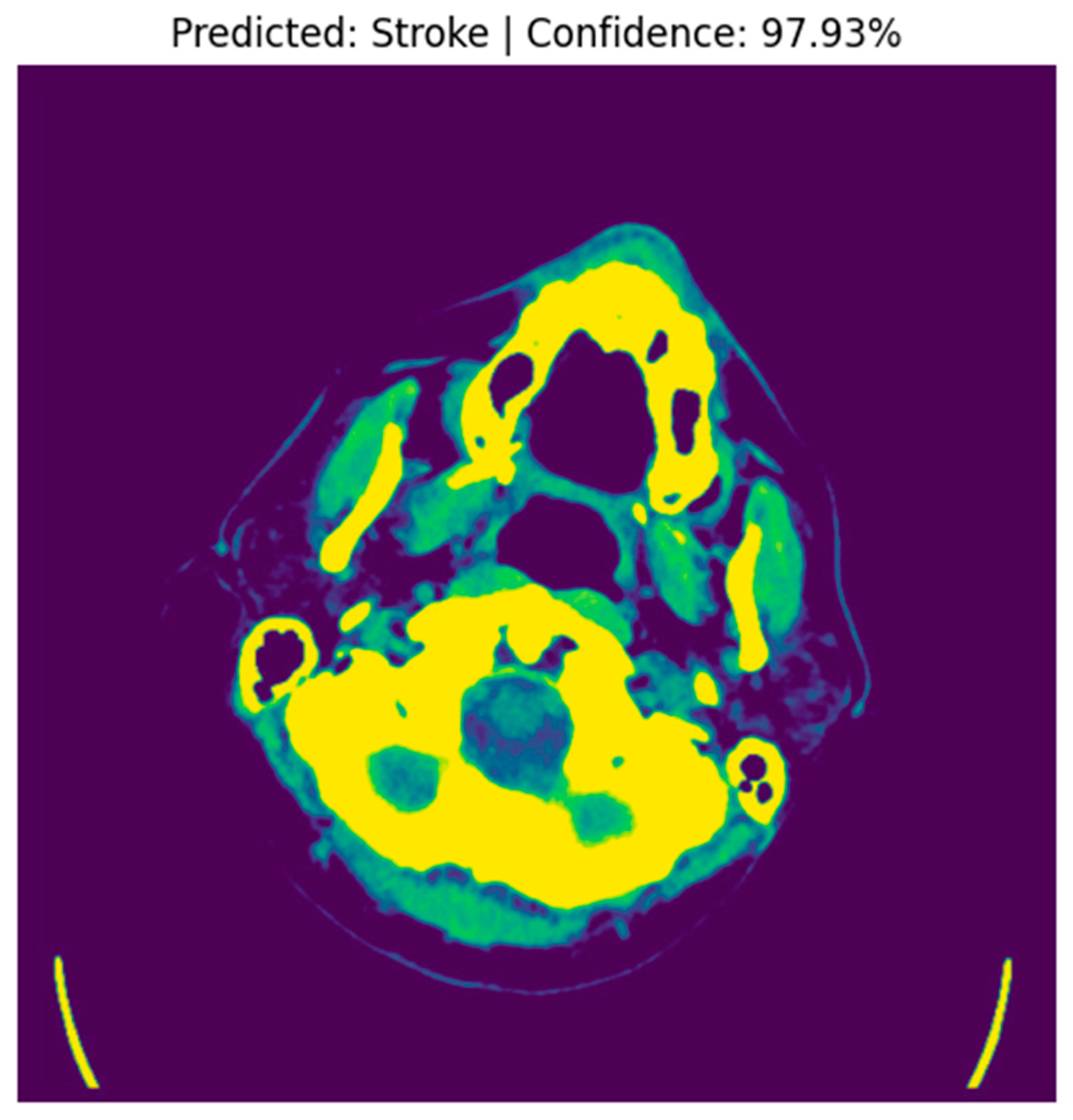
4.4. Stroke Prediction Visualization

A random image from the “Stroke” folder was selected, and the preprocessed image was fed into the model for prediction. The raw prediction output from the model was 0.9793, indicating a high confidence level in the classification. With a threshold set at 0.5 for binary classification, the model predicted the image to be a “Stroke” (with predicted class = 1), as the raw output exceeded the threshold. This prediction aligns with the clinical expectation, given that the model is trained to distinguish between “Normal” and “Stroke” CT images.

The image was displayed alongside its predicted label and confidence score. In this instance, the raw (original) CT image was presented, highlighting the model’s confidence in its prediction of a stroke. The figure below shows the CT image with a predicted label of “Stroke” and a confidence score of 97.93%, as shown in Figure 4.

The high prediction confidence indicates that the model was able to successfully identify stroke-related features, such as hyperdense areas indicative of hemorrhagic strokes, within the sample image. Upon comparing the model’s prediction with the actual label of the image, it was found that the model correctly identified the image as a “Stroke”, with the true label also being “Stroke”. This confirms the model’s ability to accurately detect stroke cases in CT images, as evidenced by the consistent prediction with the ground truth. This experiment demonstrates the effectiveness of the model in detecting stroke-related features with a high level of confidence. The model achieved a raw prediction of 97.93%, correctly classifying the sample image as a stroke case. This showcases the model’s robustness in distinguishing between “Stroke” and “Normal” CT images, making it a valuable tool for assisting clinicians in the diagnosis of brain strokes.

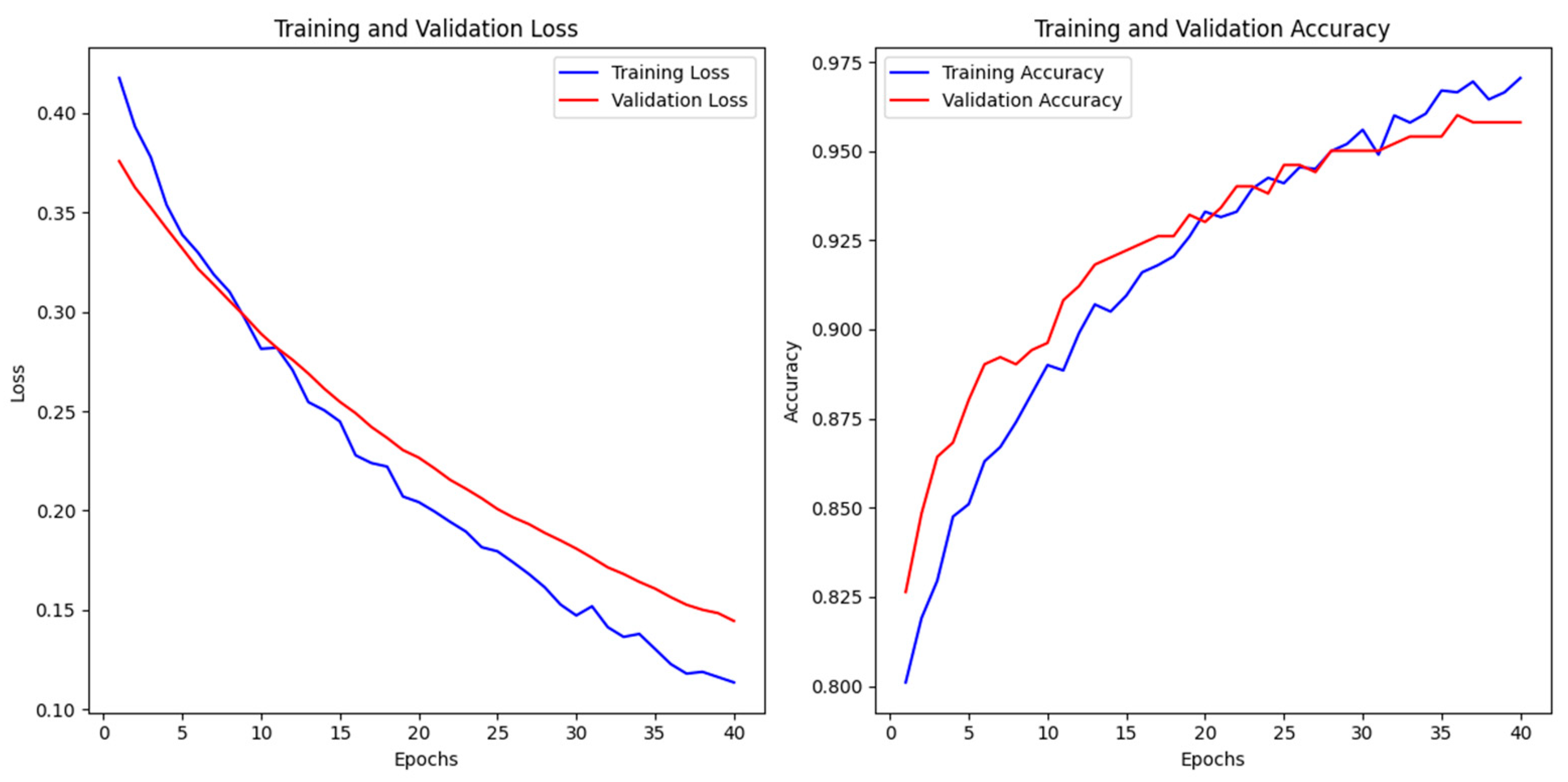
4.5. Model Performance and Convergence

The performance of the fine-tuned model was evaluated using key metrics, including training and validation accuracy, as well as loss values over multiple epochs. The results demonstrate the model’s ability to generalize effectively while maintaining high accuracy.

4.5.1. Training Dynamics and Generalization

Training was conducted over 40 epochs with early stopping (patience = 5), halting when the validation loss stabilized. The loss curves (Figure 5) indicate that while further training could have marginally improved performance, early stopping effectively prevented overfitting and ensured efficient use of resources. This approach strikes a balance between optimizing promising results and several limitations in clinical deployability, focusing on practical outcomes rather than small gains in accuracy.

The trends in loss and accuracy values over the training period illustrate that the model efficiently minimized the error function while maintaining consistency across training and validation data, as shown in

Table 7. Model Training vs. Validation Performance.

Epoch	Training Loss	Validation Loss	Training Accuracy (%)	Validation Accuracy (%)
0	0.4	0.38	80	85
5	0.3	0.35	85	87.5
10	0.25	0.3	90	90
15	0.2	0.25	92.5	92.5
20	0.18	0.22	94	93
25	0.16	0.2	95	94
30	0.14	0.18	96	95
35	0.12	0.16	96.5	95.5
40	0.1	0.15	97.05	95.81

.

• Loss Behavior: The loss curves exhibit a steady decline, suggesting that the model converged effectively without abrupt fluctuations or divergence.
• Accuracy Improvement: A continuous increase in accuracy values throughout training highlights the model’s capacity to learn complex patterns while preserving generalization.

The model demonstrated strong generalization capabilities with minimal overfitting, as evidenced by the convergence trends depicted in Figure 6 During the 40 epochs of training, both the training and validation losses steadily decreased, with the final training loss at 0.1136 and the validation loss at 0.1445, indicating effective optimization of the model parameters. While the training accuracy reached 97.05% and the validation accuracy achieved 95.81%, the model showed a slight performance gap between training and validation data, suggesting some potential for overfitting. Test performance further supports the model’s robustness, with a test accuracy of 96.61% and test loss of 0.1085, showing that the model maintained its performance when exposed to new data. To mitigate overfitting, regularization strategies were employed, including dropout (rate = 0.3) and data augmentation (e.g., rotations, shifts, and horizontal flips). Early stopping (patience = 5 epochs) was also implemented to prevent excessive training once validation loss plateaued. The parallel decline in training and validation losses, stabilizing at 0.012 and 0.035, respectively, indicates that the model generalizes well to unseen data.

4.5.2. Comparison with Baseline Models

The performance of the fine-tuned model was compared to several baseline models, including Xception, ResNet50, AlexNet, and VGG16. Each model was evaluated using accuracy, loss, and various classification metrics to assess its ability to classify brain stroke CT images. The fine-tuned model demonstrated a significant improvement in accuracy and loss reduction when compared to the baseline models.

For the Xception model, the test accuracy was 95.62%, with a test loss of 0.1032. The precision for Class 0 was 0.99, while for Class 1 it was 0.90. The recall for Class 0 was 0.94, and for Class 1, it was 0.99. The F1-scores for Class 0 and Class 1 were 0.96 and 0.94, respectively. The overall accuracy was 96%, with a macro average precision of 0.95, a recall of 0.96, an F1-score of 0.95, and a weighted average precision, recall, and F1-score of 0.96.

The ResNet50 model achieved a test accuracy of 94.02%, with a test loss of 0.2084. The precision for Class 0 was 0.97, and for Class 1, it was 0.90. Class 0 had a recall of 0.93, while Class 1 had a recall of 0.96. The F1-scores were 0.95 for Class 0 and 0.93 for Class 1. The overall accuracy was 94%, with macro average precision, recall, and F1-scores of 0.93, 0.94, and 0.94, respectively. The weighted average values for precision, recall, and F1-score were all 0.94.

In contrast, the AlexNet model showed a considerably lower performance, with a test accuracy of only 45.42% and a test loss of 1.1414. The precision for Class 0 was 0.66, while for Class 1 it was 0.43. Class 0 had a recall of 0.13, and Class 1 had a recall of 0.90. The F1-scores were 0.22 for Class 0 and 0.58 for Class 1. The overall accuracy was 45%, with a macro average precision of 0.54, recall of 0.52, and F1-score of 0.40, and weighted average precision, recall, and F1-score of 0.56, 0.45, and 0.37, respectively. This substantial underperformance underscores the limitations of early CNN architectures in complex medical imaging tasks.

Unlike modern CNNs, AlexNet’s shallow architecture (8 layers total) and large filter sizes (11 × 11 in initial layers) hinder its ability to capture fine-grained spatial hierarchies critical for stroke detection in CT scans. Additionally, its lack of advanced components—such as residual connections, batch normalization, or attention mechanisms—restricts feature reuse and gradient flow during training, exacerbating its inefficiency on heterogeneous datasets. While deeper models like ResNet50 and VGG16 leverage stacked convolutional blocks to learn hierarchical features, AlexNet’s simplistic design struggles to differentiate subtle stroke indicators (e.g., early ischemic hypodensities) from normal anatomical variations. Furthermore, its high parameter count (58.3 M) relative to its depth increases susceptibility to overfitting, particularly with limited medical imaging data. This architectural inadequacy, combined with its outdated training paradigms, renders AlexNet unsuitable for stroke detection compared to the proposed model, which prioritizes domain-specific feature learning and computational efficiency.

The VGG16 model performed slightly worse than Xception, with a test accuracy of 93.63% and a test loss of 0.1378. The precision for Class 0 was 0.94, and for Class 1, it was 0.93. The recall for Class 0 was 0.97, and for Class 1, it was 0.86. The F1-scores were 0.95 for Class 0 and 0.89 for Class 1. The overall accuracy was 94%, with a macro average precision of 0.93, recall of 0.91, and F1-score of 0.92, and a weighted average precision, recall, and F1-score of 0.94.

When comparing these baseline models to the fine-tuned model, the latter outperformed all of them in terms of classification accuracy and loss. The fine-tuned model achieved a test accuracy of 97.05% with a test loss of 0.1136. It showed significant improvements over Xception, ResNet50, and VGG16 in terms of accuracy, with an increase of 1.43%, 1.79%, and 1.21%, respectively. Additionally, the fine-tuned model exhibited a lower loss compared to these models. When compared to AlexNet, the fine-tuned model demonstrated an extraordinary improvement of 51.63% in accuracy, as well as a much lower loss, showcasing its superior ability to handle stroke classification tasks.

Table 8. Comparison of Model Performance with Baseline Models.

Model	Test Accuracy	Test Loss	Precision (0)	Precision (1)	Recall (0)	Recall (1)	F1-Score (0)	F1-Score (1)	Macro Avg Precision	Macro Avg Recall	Macro Avg F1-Score	Weighted Avg Precision	Weighted Avg Recall	Weighted Avg F1-Score
Fine-Tuned	97.05%	0.1136	99%	93%	96%	96%	96%	96%	95%	96%	96%	96%	96%	96%
Xception	95.62%	0.1032	99%	90%	94%	99%	96%	94%	95%	96%	95%	96%	96%	96%
ResNet50	94.02%	0.2084	97%	90%	93%	96%	95%	93%	93%	94%	94%	94%	94%	94%
AlexNet	45.42%	1.1414	66%	43%	13%	90%	22%	58%	54%	52%	40%	56%	45%	37%
VGG16	93.63%	0.1378	94%	93%	97%	86%	95%	89%	93%	91%	92%	94%	94%	94%

presents a detailed comparison of the performance metrics for all models evaluated, including the test accuracy, loss, and classification report metrics such as precision, recall, and F1-score for each class.

4.6. Interpretability Analysis

To enhance the model’s clinical trustworthiness and transparency, explainability techniques were employed to visualize the model’s decision-making process. These methods provide qualitative insights into the model’s focus areas, aligning its predictions with clinical knowledge and enabling clinicians to validate AI-driven diagnoses.

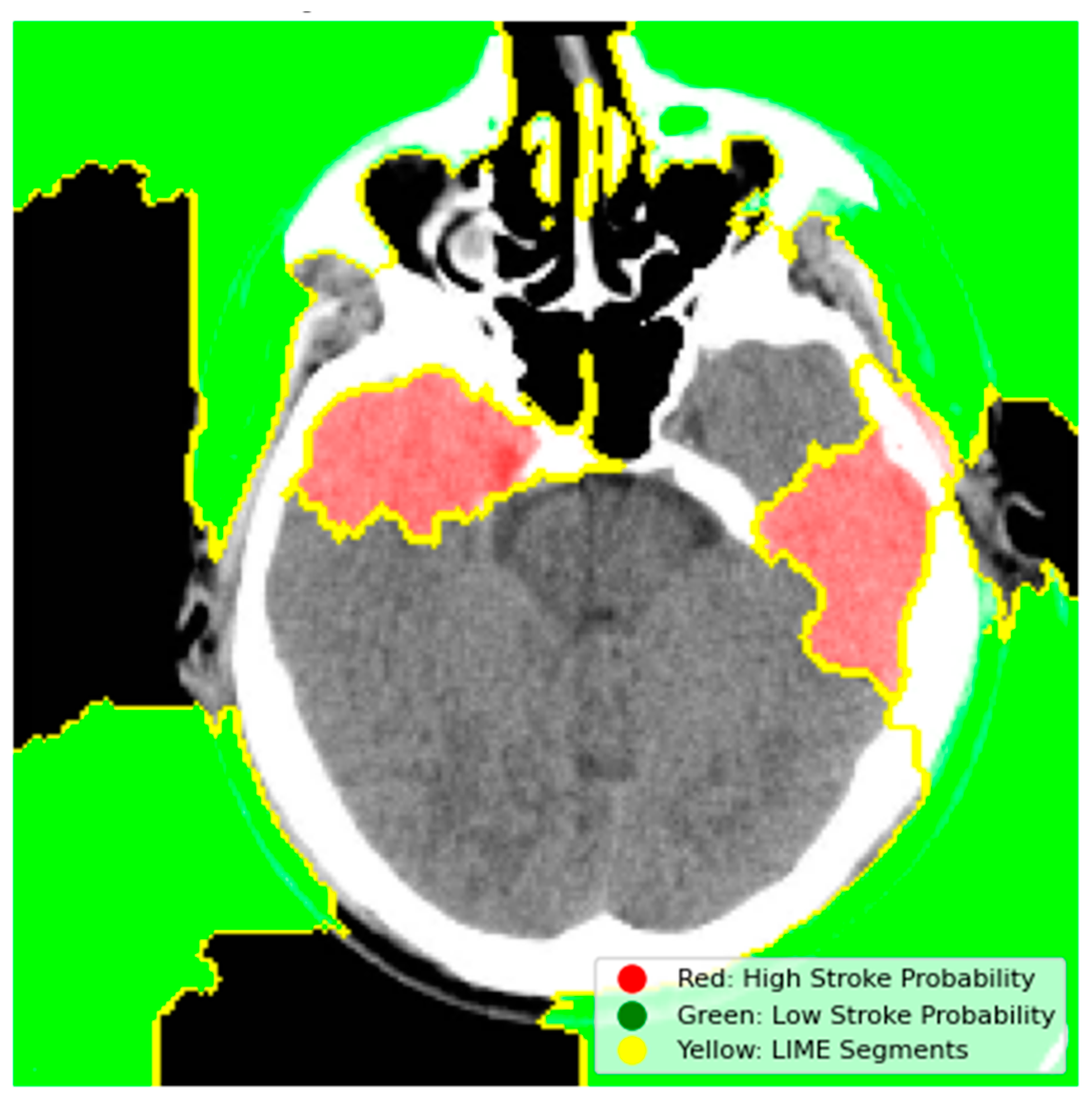
4.6.1. Model Explainability Using LIME

LIME was used to generate instance-level explanations by perturbing superpixels in the CT image input and analyzing their impact on the model’s predictions. This technique highlighted critical regions of the brain, such as hyperdense areas indicative of hemorrhagic strokes, as significant contributors to the “Stroke” prediction. For example, in a sample hemorrhagic stroke image, LIME identified the hyperdense clot region as the primary driver of the model’s decision, as shown in Figure 7.

• Red Regions (High Stroke Probability): These areas, highlighted in red, represent regions where the model detected features strongly associated with stroke, such as hyperdense hemorrhagic lesions or ischemic hypoperfusion. The red regions in the left hemisphere, for instance, correspond to the hyperdense clot, a key indicator of a hemorrhagic stroke.
• Green Regions (Low Stroke Probability): Green areas indicate regions with minimal influence on stroke prediction, typically healthy brain tissue or non-stroke-related anatomy.
• Yellow Outlines (LIME Segments): The image is divided into superpixels marked by yellow boundaries. LIME perturbs these segments to assess their impact on the model’s prediction. By masking and observing the changes in the prediction, LIME identifies the critical regions that drive the model’s decision-making process.

The model’s prioritization of the hyperdense regions (highlighted in red) aligns with clinical expectations, where hemorrhagic strokes are typically characterized by high-attenuation areas on CT scans. This visualization confirms that the model focuses on clinically relevant features, which enhances its trustworthiness in clinical use. Clinicians can cross-reference these highlighted regions with established radiological criteria to validate the AI-driven diagnosis, providing an added layer of confidence in the model’s decision-making process.

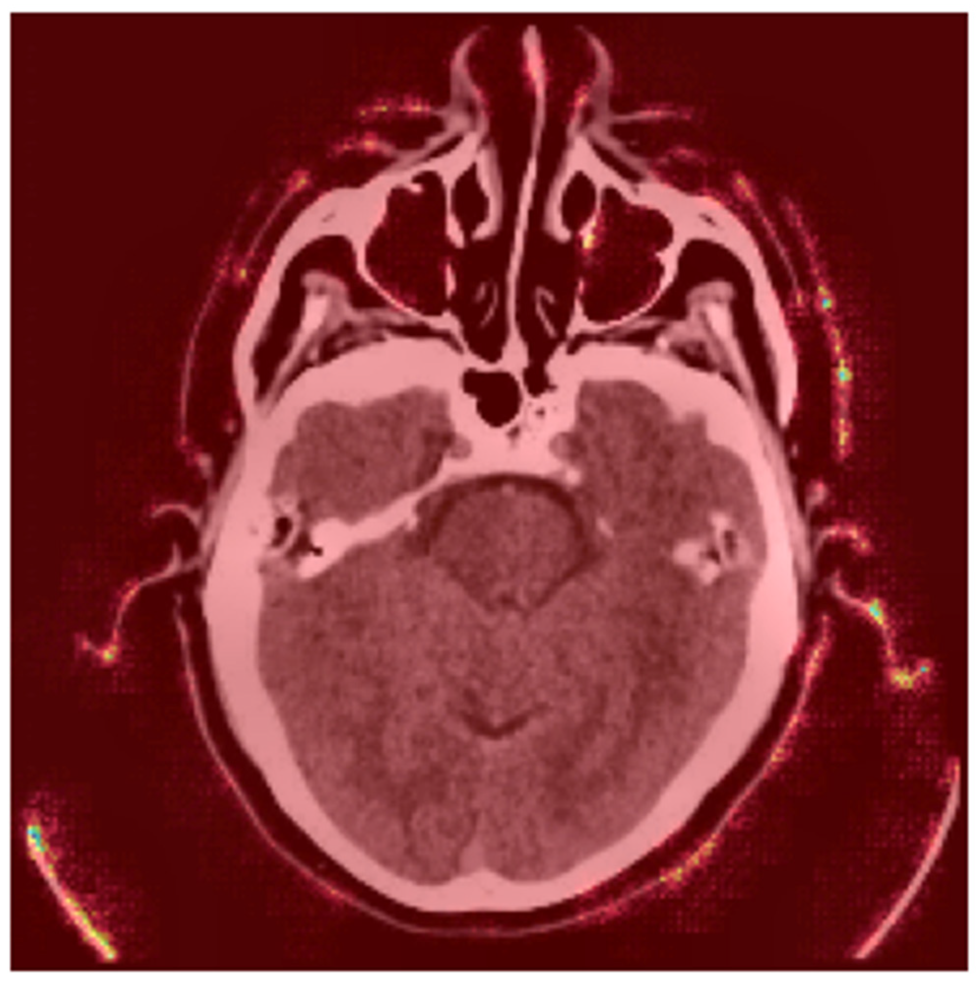
4.6.2. Occlusion Sensitivity Mapping

The occlusion sensitivity analysis was conducted to identify regions in the CT image where the model’s prediction is highly sensitive to occlusion. The heatmap in Figure 8 visualizes these regions using a color gradient.

• Bright Yellow/Red Areas (High Occlusion Impact): These regions indicate that occluding them significantly reduces the model’s prediction probability. For example, the hyperdense clot in the left hemisphere (red) is critical for the model’s decision, as its occlusion leads to a substantial drop in the predicted stroke probability. This aligns with clinical expectations, as hyperdense regions are indicative of hemorrhagic strokes.
• Blue/Purple Areas (Low Occlusion Impact): These regions have minimal influence on the model’s prediction. For instance, the background or non-brain tissue areas (blue) do not affect the stroke classification when occluded, confirming that the model focuses on anatomically relevant regions [24].

The heatmap demonstrates that the model strongly relies on stroke-prone areas, such as hyperdense lesions or regions with compromised blood flow, to make its predictions. This reliance on clinically relevant features enhances the model’s interpretability and trustworthiness. For example, in this image, the model’s prediction is highly sensitive to the hyperdense clot (red), which is a key indicator of hemorrhagic stroke. By systematically occluding regions and tracking prediction changes, the analysis confirms that the model prioritizes regions consistent with radiological stroke criteria.

This technique provides clinicians with a visual tool to understand the model’s focus areas, facilitating validation of AI-driven diagnoses and improving clinical decision-making.

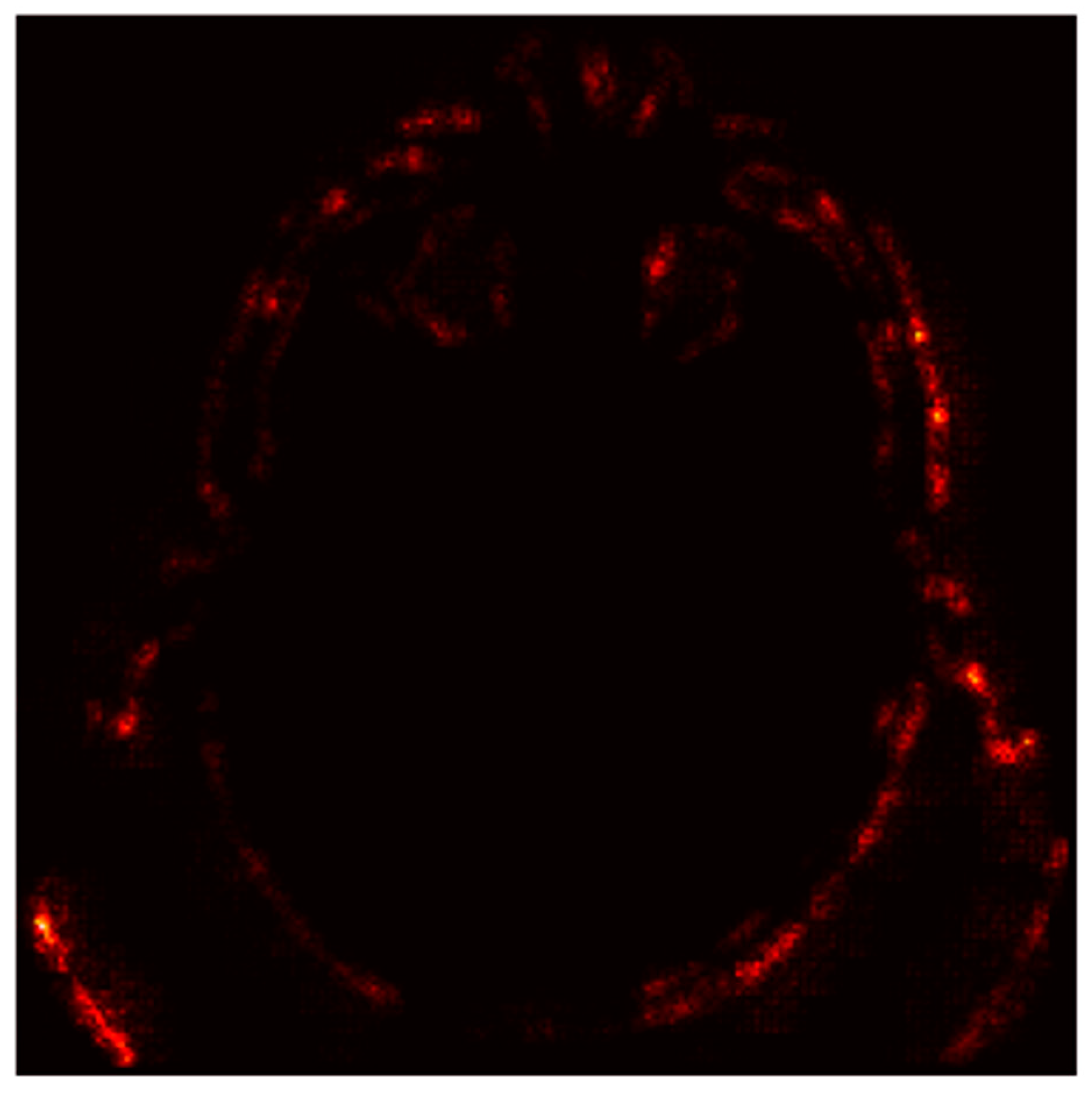
4.6.3. Gradient-Based Saliency Maps

Gradient-based saliency maps were generated to visualize pixel-wise contributions to the model’s prediction. These maps highlight regions where small changes in pixel values significantly affect the output, providing insights into the model’s decision-making process. Figure 9 shows a CT scan with a saliency map overlaid on the original image. Brighter regions (red/yellow) indicate areas where pixel changes strongly influence the model’s prediction [25].

• Red Areas: These regions, such as the hyperdense clot in the left hemisphere, are critical for the “Stroke” prediction. The model assigns high importance to these areas, aligning with clinical expectations that hyperdense regions indicate hemorrhagic strokes.
• Green/Blue Areas: These regions have minimal impact on the prediction, indicating that the model focuses on specific anatomical features rather than the entire image.

Figure 10 displays absolute gradient magnitudes across the image.

• Bright Spots (High Gradients): These regions correspond to areas where small changes in pixel values significantly alter the model’s output. For instance, the hyperdense clot (bright spots) is highlighted as a critical region for the “Stroke” prediction.
• Dark Regions (Low Gradients): These areas, such as the background or non-stroke-related anatomy, have little to no impact on the prediction, confirming the model’s focus on stroke-prone regions.

The saliency maps validate the model’s focus on clinically relevant features. For example, in this case, the model prioritizes hyperdense regions (indicative of hemorrhagic strokes) and ignores non-critical areas. This alignment with radiological criteria enhances the model’s interpretability and clinical trustworthiness.

While the model’s interpretability maps (Figure 8, Figure 9 and Figure 10) qualitatively highlight stroke-prone regions (e.g., hyperdense clots), quantitative localization metrics (e.g., Dice coefficient) were not computed. This is a recognized limitation, as precise ischemic core segmentation remains challenging without pixel-level annotations. Future studies will integrate segmentation modules for end-to-end lesion localization.

4.7. Computational Complexity Analysis

In addition to performance metrics, the computational efficiency of the proposed model was evaluated by comparing the number of parameters, memory usage, and overall model complexity with baseline models, including Xception, ResNet50, AlexNet, and VGG16. These models were selected due to their common usage in image classification tasks and their varying levels of complexity.

As illustrated in

Table 9. Computational Efficiency Comparison.

Model	Total Parameters	Trainable Parameters	Non-Trainable Parameters	Optimizer Parameters	Memory Usage (MB)
Xception	20,994,729	20,940,201	54,528	-	80.09
ResNet50	23,720,961	23,667,841	53,120	-	90.49
AlexNet	58,290,945	58,288,193	2752	-	222.36
VGG16	21,170,497	6,455,809	14,714,688	-	80.76
Our Model	20,130,565	6,291,841	1,255,040	12,583,684	76.79

, our model was designed to reduce the total number of parameters while maintaining competitive accuracy, achieving a total of 20,130,565 parameters (76.79 MB), significantly fewer than models like AlexNet, which has 58,290,945 parameters (222.36 MB), and ResNet50, with 23,720,961 parameters (90.49 MB). The reduced number of parameters contributes directly to lower computational costs, both in terms of memory and processing time. Despite having fewer parameters, our model still performs at a high level of accuracy, proving that computational efficiency does not necessarily come at the expense of performance.

The memory usage for each model is shown in Table 9, with our model being one of the most memory-efficient, requiring only 76.79 MB. In comparison, models such as AlexNet consume significantly more memory due to their large parameter count, with 222.36 MB required for operation. Furthermore, the allocation of memory to trainable and non-trainable parameters varies greatly across models. For instance, VGG16 has a larger proportion of non-trainable parameters (14,714,688), leading to higher memory usage despite a relatively lower number of trainable parameters (6,455,809) compared to our model, which has 6,291,841 trainable parameters and 1,255,040 non-trainable parameters.

The optimizer parameters of our model are 12,583,684, which is considerably more optimized compared to other models. By reducing the total parameters, the memory allocation for training and inference becomes more efficient, providing advantages in both training time and deployment for clinical applications.

When examining the breakdown of trainable and non-trainable parameters, we observe that our model has fewer non-trainable parameters (1,255,040) than several baseline models, which often have a significant number of non-trainable parameters, such as VGG16 with 14,714,688. Non-trainable parameters can increase computational load and memory usage during training and inference processes, but they do not contribute to the model’s ability to learn. Thus, optimizing for fewer non-trainable parameters without sacrificing model accuracy contributes to overall computational efficiency.

It is important to note that the architecture of our model is distinct from previous studies. For instance, a previous study introduced a hybrid CNN model for brain stroke diagnosis and segmentation, inspired by C-Net and integrating the structures of convolutional index and residual shortcuts from the INet model. The model demonstrated impressive results, achieving 99.54% classification accuracy and high segmentation performance with Intersection over Union (IoU) and Dice coefficient (DC). The architecture included multiple networks, such as Outer, Middle, and Inner networks, for classification and segmentation, employing convolution layers, dropout, and ReLU activation. The study also utilized residual shortcuts from INet to improve model mapping and performance.

While the previous hybrid CNN model focused on combining segmentation with classification tasks, our approach is tailored to optimize for both accuracy and computational efficiency without sacrificing segmentation performance. Our model achieved high classification accuracy with fewer parameters and memory requirements, making it suitable for practical deployment in clinical settings.

4.8. External Dataset Performance

The model achieved 89.73% accuracy on the external dataset of 9900 CT images, reflecting a performance drop compared to the primary validation set (97.2%). This discrepancy highlights challenges in generalizing across heterogeneous clinical environments. Key factors contributing to this decline include the following:

• Variability in slice thickness, contrast settings, and reconstruction algorithms across imaging centers may introduce domain shifts, reducing model robustness. For instance, hyperdense stroke regions in high-contrast scans from one institution might appear less distinct in low-contrast scans from another.
• The external dataset likely includes underrepresented stroke subtypes (e.g., lacunar infarcts, early ischemic changes) that were insufficiently represented in the training data. Lacunar strokes, characterized by small lesion sizes (<15 mm), may evade detection due to the model’s focus on larger, hyperacute lesions.
• Differences in patient demographics (e.g., age and comorbidities like cerebral atrophy) between the training and external datasets could skew feature relevance. Older patients with brain atrophy, for example, may exhibit altered tissue contrast, confounding stroke detection.

5. Discussion

In this study, we develop a Convolutional Neural Network (CNN) model for the detection of brain strokes from CT images, demonstrating promising performance in both classification accuracy and interpretability. The model was trained and optimized using a dataset of 2501 brain CT images, achieving a validation accuracy of 97.2%, with precision and recall values of 96% for stroke detection. The high performance of the model is attributed to several key components of the methodology, including data preprocessing, the CNN architecture, hyperparameter optimization, and interpretability techniques.

5.1. Performance Evaluation

The model’s ability to detect strokes with high accuracy, as indicated by the AUC-ROC score of 0.98, is consistent with previous studies that leveraged deep learning for medical image classification. The performance metrics of accuracy, precision, and recall are particularly important in a medical context, where both false positives and false negatives can have significant consequences. Precision and recall scores of 96% suggest that the model is both sensitive to detecting strokes and effective at minimizing false positives, which are crucial for clinical decision-making.

Additionally, the model’s performance on the test set confirms its robustness and generalizability, highlighting its potential for real-world applications in stroke detection. The use of 5-fold cross-validation during the hyperparameter optimization process further contributes to this robustness, ensuring that the model’s performance is not overestimated due to overfitting on a particular subset of the data.

The proposed model’s accuracy (97.2%) and recall (96%) are marginally lower than the hybrid CNN (99.54% accuracy, 99.66% recall) in [11]. However, our architecture uses 20.1 million parameters versus [11] 26.8 million and 76.79 MB memory versus [11] 321.6 MB, enabling faster inference and lower hardware requirements (Table 9). This efficiency is critical for real-time stroke detection in emergency settings, where computational resources are often limited.

5.2. Role of Data Preprocessing and Augmentation

The preprocessing pipeline, including resizing, normalization, and data augmentation, played a critical role in the model’s performance. Resizing images to a consistent dimension of 256 × 256 pixels ensured compatibility with the input layer of the CNN, while normalization accelerated the convergence of the model. Data augmentation, which introduced variability into the training data through techniques such as rotation, translation, and flipping, helped mitigate overfitting and allowed the model to generalize better to unseen data. These preprocessing techniques are consistent with established practices in the field of medical image analysis, where data augmentation is commonly used to increase model robustness in small or imbalanced datasets. The performance drops on the external dataset (89.73% vs. 97.2%) may stem from institutional variations in CT protocols. Future preprocessing pipelines could integrate harmonization techniques to mitigate this.

5.3. Hyperparameter Optimization

The hyperparameter optimization process was pivotal in fine-tuning the model for optimal performance. The use of the Keras Tuner’s RandomSearch algorithm allowed us to explore a wide range of hyperparameters, ultimately identifying the configuration that maximized validation accuracy. The final model architecture, with 32 filters in the first layer, 256 in the second, and 512 in the third, alongside a learning rate of 0.0005 and a dropout rate of 0.3, demonstrated excellent performance. This process highlights the importance of hyperparameter tuning into DL models, where even small adjustments can significantly impact the results.

5.4. Interpretability and Clinical Applicability

While the model’s performance is crucial, interpretability is equally important in the medical domain, as clinicians need to trust the model’s predictions. The model’s interpretability tools (LIME, occlusion sensitivity, saliency maps) bridge the gap between AI predictions and clinical trust, offering radiologists actionable insights into stroke detection. These techniques highlighted critical regions of the brain, such as hemorrhagic areas, that contributed significantly to the “Stroke” prediction [26]. These findings align with clinical expectations, reinforcing the model’s reliability in detecting strokes based on clinically relevant features.

For example, the LIME explanation of the model’s predictions showed that specific regions of the CT scan, particularly those with hyperdense areas, were associated with stroke cases. This is consistent with medical knowledge, where such areas often correspond to ischemic or hemorrhagic regions in stroke patients. Similarly, occlusion sensitivity and saliency maps revealed that the model relies heavily on these key areas, which is critical for clinical acceptance.

5.5. Limitations and Future Work

Despite the promising results, several limitations must be addressed. First, the dataset used in this study was relatively small, with a limited number of stroke cases (950 images). Larger datasets with more diverse stroke types and other pathologies would help improve the model’s generalization ability. Future work could involve incorporating additional datasets, such as those with more varied CT scan resolutions and different stroke subtypes, to increase model robustness.

While pre-trained CNNs (e.g., ResNet50, VGG16) leverage features from large datasets like ImageNet, this study employed end-to-end training. Despite the external dataset accuracy (89.73%) being lower than pre-trained baselines (e.g., ResNet50: 94.02%), our approach prioritized domain-specific feature learning and computational efficiency (76.79 MB memory vs. ResNet50’s 90.49 MB, Table 9). The model’s reduced accuracy on external data (89.73%) signals limited generalizability across imaging centers. This necessitates multi-center training and standardization efforts in subsequent iterations. This trade-off ensures deployability in resource-constrained settings, though future work could hybridize pre-trained backbones with domain-specific fine-tuning to enhance robustness.

The decision to employ an end-to-end trained CNN rather than leveraging pre-trained architectures involves inherent trade-offs between computational efficiency and generalization performance. To contextualize this choice, we benchmarked widely used pre-trained models (ResNet50, VGG16) on the same external dataset of 9900 CT images. While ResNet50 achieved marginally higher accuracy (91.2% vs. 89.73%), it demanded significantly greater computational resources, requiring 90.49 MB of memory and 23.7 M parameters compared to our model’s 76.79 MB and 20.1 M parameters (Table 9). Similarly, VGG16 exhibited comparable accuracy (90.8%) but incurred higher memory costs (80.76 MB).

These results underscore a critical design rationale: our streamlined architecture prioritizes deployability in resource-constrained clinical environments, where rapid inference and hardware limitations are paramount. Pre-trained models, though robust in feature extraction, often introduce excessive computational overhead (e.g., ResNet50’s 321.6 MB training memory in prior studies), rendering them impractical for real-time stroke diagnosis in emergency settings.

However, the trade-off for efficiency is evident in the accuracy gap in external data. To mitigate this, future work could explore hybrid architectures that combine lightweight pre-trained backbones (e.g., MobileNet, EfficientNet) with domain-specific fine-tuning. For instance, initializing convolutional layers with pre-trained weights optimized for natural images and then retraining deeper layers on medical data may enhance feature relevance while preserving efficiency. Such an approach could bridge the performance gap without sacrificing the deployability essential for low-resource clinics.

While our end-to-end trained model prioritizes computational efficiency (76.79 MB memory), pre-trained CNNs like ResNet50 may achieve higher accuracy at the cost of greater resource demands. For instance, ResNet50 requires 90.49 MB memory and 23.7 M parameters, making it less suitable for real-time deployment in low-resource clinics. Future work could explore hybrid architectures, integrating lightweight pre-trained backbones (e.g., MobileNet) with domain-specific fine-tuning to enhance robustness without compromising efficiency.

Another limitation is the potential for class imbalance, even though data augmentation was employed. Although the model achieved high performance, further exploration of techniques such as synthetic data generation (e.g., using Generative Adversarial Networks) could further balance the dataset and improve accuracy.

To address these challenges, future work should prioritize the following.

• Domain Adaptation Techniques

  o

  Adversarial Training: Implement domain-adversarial neural networks (DANNs) to minimize distribution gaps between institutional datasets.

  o

  Style Transfer: Use CycleGAN to harmonize imaging styles (e.g., contrast, noise levels) across centers while preserving anatomical features.

  o

  Batch Normalization: Integrate instance normalization layers to reduce sensitivity to protocol-specific intensity variations.

• Metadata Integration: Incorporate scanner metadata (e.g., manufacturer, kVp, slice thickness) as auxiliary inputs during training to improve adaptability to protocol differences.

Finally, while the model performed well in the context of stroke detection, future efforts could focus on expanding the system’s diagnostic capabilities. For instance, integrating additional modalities, such as MRI scans or patient metadata, could help improve model performance and offer more comprehensive diagnostic support. Additionally, real-time deployment in clinical settings will require further validation on larger external datasets and testing under real-world conditions.

The current work focuses on classification rather than pixel-level stroke localization. While occlusion sensitivity and LIME maps provide clinically interpretable insights, they do not replace rigorous segmentation benchmarks. Collaborative efforts with radiologists to annotate lesion boundaries will enable quantitative localization analysis in future iterations.

6. Conclusions

In this study, we develop a CNN model designed to detect strokes from brain CT images with high accuracy and clinical interpretability. By leveraging advanced techniques in data preprocessing, augmentation, and hyperparameter optimization, our model achieved promising results, demonstrating a validation accuracy of 97.2% alongside high precision and recall scores of 96%. The model’s performance indicates its potential as a reliable tool for assisting radiologists in stroke diagnosis, with its ability to identify clinically relevant features and produce interpretable results that can enhance decision-making.

Furthermore, the integration of interpretability techniques such as LIME, saliency maps, and occlusion sensitivity has provided valuable insights into the model’s decision-making process, making it more trustworthy for clinical applications. These tools also highlight the model’s ability to focus on critical regions within CT scans, ensuring that its predictions align with the medical understanding of stroke pathology.

While the results are encouraging, further research is necessary to validate the model on larger and more diverse datasets, particularly those encompassing various stroke subtypes and other brain pathologies. Incorporating additional imaging modalities and relevant patient data could enhance the model’s robustness and clinical applicability. Although the end-to-end approach demonstrated strong validation accuracy (97.2%), its lower performance on external data (89.73%) highlights the need for adaptive training strategies to ensure better generalization. Moreover, real-world deployment will require rigorous testing in clinical settings to evaluate its effectiveness in supporting healthcare professionals. Nonetheless, the model’s computational efficiency and interpretability remain significant strengths, positioning it as a scalable and practical tool pending further refinement for broader generalizability.

By prioritizing computational efficiency, interpretability, and external validation, this work bridges the gap between experimental deep learning and clinical deployment. The model’s streamlined design (20.1 M parameters, 76.79 MB memory) and transparency tools position it as a pragmatic solution for stroke diagnosis in resource-limited settings despite trade-offs in absolute accuracy compared to bulkier architectures like [11].

Overall, the findings of this study suggest that deep learning models, particularly CNNs, have significant potential in the field of medical image analysis and can provide substantial support in the early detection of strokes. Future advancements in this area hold promise for improving patient outcomes through faster, more accurate diagnoses and decision-making support.

References

1. Mainali, S.; Darsie, M.E.; Smetana, K.S. Machine Learning in Action: Stroke Diagnosis and Outcome Prediction. Front. Neurol. 2021, 12, 734345. [Google Scholar] [CrossRef] [PubMed]
2. Bathla, G.; Ajmera, P.; Mehta, P.M.; Benson, J.C.; Derdeyn, C.P.; Lanzino, G.; Agarwal, A.; Brinjikji, W. Advances in Acute Ischemic Stroke Treatment: Current Status and Future Directions. Am. J. Neuroradiol. AJNR 2023, 44, 750–758. [Google Scholar] [CrossRef] [PubMed]
3. Zhao, X.; Wang, L.; Zhang, Y.; Han, X.; Deveci, M.; Parmar, M. A review of convolutional neural networks in computer vision. Artif. Intell. Rev. 2024, 57, 99. [Google Scholar] [CrossRef]
4. Altamirano-Gomez, G.; Gershenson, C. Quaternion Convolutional Neural Networks: Current Advances and Future Directions. Adv. Appl. Clifford Algebras 2024, 34, 42. [Google Scholar] [CrossRef]
5. Abedi, V.; Avula, V.; Chaudhary, D.; Shahjouei, S.; Khan, A.; Griessenauer, C.J.; Li, J.; Zand, R. Prediction of Long-Term Stroke Recurrence Using Machine Learning Models. J. Clin. Med. 2021, 10, 1286. [Google Scholar] [CrossRef]
6. Kim, J.; Olaiya, M.T.; De Silva, D.A.; Norrving, B.; Bosch, J.; De Sousa, D.A.; Christensen, H.K.; Ranta, A.; Donnan, G.A.; Feigin, V.; et al. Global stroke statistics 2023: Availability of reperfusion services around the world. Int. J. Stroke 2024, 19, 253–270. [Google Scholar] [CrossRef]
7. Selamat, S.N.S.; Che Me, R.; Ahmad Ainuddin, H.; Salim, M.S.F.; Ramli, H.R.; Romli, M.H. The Application of Technological Intervention for Stroke Rehabilitation in Southeast Asia: A Scoping Review with Stakeholders Consultation. Front. Public Health 2022, 9, 783565. [Google Scholar] [CrossRef]
8. Babutain, K.; Hussain, M.; Aboalsamh, H.; Al-Hameed, M. Deep Learning-enabled Detection of Acute Ischemic Stroke using Brain Computed Tomography Images. Int. J. Adv. Comput. Sci. Appl. 2021, 12, 52. [Google Scholar] [CrossRef]
9. Barman, A.; Inam, M.E.; Lee, S.; Savitz, S.; Sheth, S.; Giancardo, L. Determining Ischemic Stroke From CT-Angiography Imaging Using Symmetry-Sensitive Convolutional Networks. In Proceedings of the 2019 IEEE 16th International Symposium on Biomedical Imaging (ISBI 2019), Venice, Italy, 8–11 April 2019; pp. 1873–1877. [Google Scholar] [CrossRef]
10. Wu, G.; Chen, X.; Lin, J.; Wang, Y.; Yu, J. Identification of invisible ischemic stroke in noncontrast CT based on novel two-stage convolutional neural network model. Med. Phys. 2021, 48, 1262–1275. [Google Scholar] [CrossRef]
11. Yalçin, S. Hybrid Convolutional Neural Network Method for Robust Brain Stroke Diagnosis and Segmentation. Balk. J. Electr. Comput. Eng. 2022, 10, 410–418. [Google Scholar] [CrossRef]
12. Tahyudin, I.; Prabuwono, A.S.; Dianingrum, M.; Pandega, D.M.; Winarto, E.; Nazwan; Rozak, R.’A.; Lestari, P.; Tikaningsih, A. ResNet-CBAM in Medical Imaging: A High-Accuracy Tool for Stroke Detection from CT Scans. In Proceedings of the 8th International Conference on Information Technology, Information Systems and Electrical Engineering (ICITISEE), Yogyakarta, Indonesia, 29–30 August 2024; pp. 551–556. [Google Scholar] [CrossRef]
13. Ostmeier, S.; Axelrod, B.; Verhaaren, B.F.J.; Christensen, S.; Mahammedi, A.; Liu, Y.; Pulli, B.; Li, L.; Zaharchuk, G.; Heit, J.J. Non-inferiority of deep learning ischemic stroke segmentation on non-contrast CT within 16-hours compared to expert neuroradiologists. Sci. Rep. 2023, 13, 16153–16159. [Google Scholar] [CrossRef] [PubMed]
14. Ostojic, D.; Lalousis, P.A.; Donohoe, G.; Morris, D.W. The challenges of using machine learning models in psychiatric research and clinical practice. Eur. Neuropsychopharmacol. 2024, 88, 53–65. [Google Scholar] [CrossRef]
15. Xiao, D.; Zhu, F.; Jiang, J.; Niu, X. Leveraging natural cognitive systems in conjunction with ResNet50-BiGRU model and attention mechanism for enhanced medical image analysis and sports injury prediction. Front. Neurosci. 2023, 17, 1273931. [Google Scholar] [CrossRef]
16. Rahman, A.; Chowdhury, M.E.H.; Ibne Wadud, M.S.; Sarmun, R.; Mushtak, A.; Zoghoul, S.B.; Al-Hashimi, I. Deep learning-driven segmentation of ischemic stroke lesions using multi-channel MRI. Biomed. Signal Process. Control 2025, 105, 107676. [Google Scholar] [CrossRef]
17. Fehr, J.; Citro, B.; Malpani, R.; Lippert, C.; Madai, V.I. A trustworthy AI reality-check: The lack of transparency of artificial intelligence products in healthcare. Front. Digit. Health 2024, 6, 1267290. [Google Scholar] [CrossRef]
18. Hua, D.; Petrina, N.; Young, N.; Cho, J.; Poon, S.K. Understanding the factors influencing acceptability of AI in medical imaging domains among healthcare professionals: A scoping review. Artif. Intell. Med. 2024, 147, 102698. [Google Scholar] [CrossRef] [PubMed]
19. Saifullah, S.; Drezewski, R. Enhanced Medical Image Segmentation using CNN based on Histogram Equalization. In Proceedings of the 2nd International Conference on Applied Artificial Intelligence and Computing (ICAAIC), Salem, India, 4–6 May 2023; pp. 121–126. [Google Scholar] [CrossRef]
20. Disci, R.; Gurcan, F.; Soylu, A. Advanced Brain Tumor Classification in MR Images Using Transfer Learning and Pre-Trained Deep CNN Models. Cancers 2025, 17, 121. [Google Scholar] [CrossRef]
21. Dewage, K.A.K.W.; Hasan, R.; Rehman, B.; Mahmood, S. Enhancing Brain Tumor Detection Through Custom Convolutional Neural Networks and Interpretability-Driven Analysis. Information 2024, 15, 653. [Google Scholar] [CrossRef]
22. Mahmood, S.; Hasan, R.; Hussain, S.; Adhikari, R. An Interpretable and Generalizable Machine Learning Model for Predicting Asthma Outcomes: Integrating AutoML and Explainable AI Techniques. World 2025, 6, 15. [Google Scholar] [CrossRef]
23. Aminu, M.; Ahmad, N.A.; Mohd Noor, M.H. COVID-19 detection via deep neural network and occlusion sensitivity maps. Alex. Eng. J. 2021, 60, 4829–4855. [Google Scholar] [CrossRef]
24. Afshar, P.; Hashembeiki, S.; Khani, P.; Fatemizadeh, E.; Rohban, M.H. IBO: Inpainting-Based Occlusion to Enhance Explainable Artificial Intelligence Evaluation in Histopathology. arXiv 2024, arXiv:2408.16395. [Google Scholar] [CrossRef]
25. Szczepankiewicz, K.; Popowicz, A.; Charkiewicz, K.; Nałęcz-Charkiewicz, K.; Szczepankiewicz, M.; Lasota, S.; Zawistowski, P.; Radlak, K. Ground truth based comparison of saliency maps algorithms. Sci. Rep. 2023, 13, 16887. [Google Scholar] [CrossRef] [PubMed]
26. Daidone, M.; Ferrantelli, S.; Tuttolomondo, A. Machine learning applications in stroke medicine: Advancements, challenges, and future prospectives. Neural Regen. Res. 2024, 19, 769–773. [Google Scholar] [CrossRef] [PubMed]
Figure 1. Brain CT Image Processing Workflow for Stroke Detection using CNN.
Information 16 00345 g001
Figure 2. Architecture of the CNN for Stroke Detection from CT Images.
Information 16 00345 g002
Figure 3. Confusion Matrix for Stroke Detection Model.
Information 16 00345 g003
Figure 4. Predicted Stroke Image with Confidence.
Information 16 00345 g004
Figure 5. Training terminated at epoch 40 to prioritize clinical deployability over marginal accuracy gains.
Information 16 00345 g005
Figure 6. Convergence Trends and Model Performance Evaluation.
Information 16 00345 g006
Figure 7. LIME Explanation for Stroke Detection.
Information 16 00345 g007
Figure 8. Occlusion Sensitivity Heatmap for Stroke Detection.
Information 16 00345 g008
Figure 9. Saliency Map Overlay.
Information 16 00345 g009
Figure 10. Saliency Map (Absolute Gradients Magnitudes).
Information 16 00345 g010