High-Frequency Cryptocurrency Price Forecasting Using Machine Learning Models: A Comparative Study

Abstract

The cryptocurrency market presents immense opportunities and significant risks due to its high volatility. Accurate price forecasting is crucial for informed investment decisions, enabling investors to optimize portfolio allocation, mitigate risk, and potentially maximize returns. Existing forecasting methods often struggle with the inherent non-stationarity and complexity of cryptocurrency price dynamics. This study addresses this challenge by developing a system for high-frequency forecasting of the closing prices of ten leading cryptocurrencies. We compare various machine learning models, including recurrent neural networks (RNNs), time series analysis (ARIMA), and conventional regression algorithms, using minute-step Bitcoin price data over a 30-day period to predict prices 60 min ahead. Our findings demonstrate that the GRU neural network exhibits superior predictive accuracy (MAPE = 0.09%, MSE = 5954.89, RMSE = 77.17, MAE = 60.20), outperforming other models considered. This improved forecasting accuracy contributes to the existing literature by providing empirical evidence for GRU’s effectiveness in the volatile cryptocurrency market and offers practical insights for investment strategies. A web application integrating the best-performing model further facilitates real-time price prediction for multiple cryptocurrencies.

1. Introduction

Cryptocurrencies have emerged as a highly attractive yet volatile investment market, attracting both experienced and new investors. This high volatility, coupled with the lack of traditional regulatory oversight and the decentralized nature of cryptocurrencies, creates unique challenges for investors seeking to make informed decisions. The inherently unpredictable nature of cryptocurrency prices, often characterized by rapid and significant fluctuations, is a key factor in this volatility. These price movements indexed over time can be modelled as non-stationary time series, meaning their statistical properties (like mean and variance) change over time, making traditional forecasting methods less effective [1].

The performance of forecasting methods depends critically on several factors: the quantity and quality of the available data, the selection of predictor attributes, and the desired forecasting horizon. Furthermore, the non-stationary nature of cryptocurrency prices means that historical patterns observed over longer time horizons (five or ten years ago) may not accurately reflect current market behavior. Conversely, relying on a very short time horizon may yield insufficient data for reliable model forecasting [2].

This study directly addresses this challenge. Our primary objective is to develop and evaluate a high-frequency cryptocurrency price forecasting system capable of predicting short-term price movements (1–4 h) with improved accuracy. We achieve this by employing various machine learning algorithms—algorithms that learn patterns from data to make predictions—including recurrent neural networks (RNNs), such as the GRU and LSTM, and more traditional time series models like ARIMA. These models are applied to minute-step price data for ten major cryptocurrencies—Bitcoin, Ethereum, Binance Coin, Cardano, Solana, XRP, Polkadot, USD Coin, Dogecoin, and Avalanche—chosen to represent a diverse portfolio regarding market presence and trading activity, thereby ensuring a comprehensive and representative dataset for our analysis. The secondary objective is to develop a user-friendly web application that integrates the best-performing model, providing accessible real-time price predictions. By providing improved forecasting accuracy, we aim to contribute practical insights to both investment strategies and the broader field of cryptocurrency price prediction.

This paper organizes the remaining sections as follows: Section 2 reviews prior research on cryptocurrency price prediction. The next section will detail the entire work methodology, which includes data acquisition, data preparation, developed prediction models, and their evaluation. In the next section, the results are discussed. The model deployment and the created web application are covered in Section 5. The final section discloses the main conclusions and prospects for future work.

2. State of the Art

For the literature review, a systematic search was conducted to identify relevant scientific papers on cryptocurrency price forecasting using machine learning techniques. The search was limited to the Springer and IEEE databases due to their comprehensive coverage of computer science, engineering, and related fields, ensuring a focus on methodologically rigorous and technically sound research. The search terms used were “cryptocurrency”, “machine learning”, and “forecasting”. To ensure relevance and quality, the following selection criteria were applied:

• Main Focus on Price Forecasting: Papers were included if they focused on cryptocurrency price forecasting using machine learning or statistical methods; however, volatility forecasting or rentability tax were also considered. Studies on other aspects of cryptocurrencies, such as security and regulation, were excluded.
• Empirical Analysis: Papers were included only if they presented empirical results based on real-world data. Theoretical studies or simulations without empirical validation were excluded.
• Peer-Reviewed Publications: Only peer-reviewed journal articles and conference proceedings were included to ensure the quality and validity of the research.
• English Language: Only papers published in English were included due to language limitations.

This process resulted in the selection of 56 papers that met the specified criteria, providing a representative overview of the current state of research in this field.

2.1. Bitcoin

Bitcoin is the first and most significant cryptocurrency on the market, being the most relevant among the selected for this study. Bitcoin was introduced in 2008 by an anonymous group under the pseudonym Satoshi Nakamoto and became operational in 2009 as an open-source network for peer-to-peer digital transactions [3]. It paved the way for Blockchain technology, which ensures transaction security through advanced cryptography. Its success led to the creation of other cryptocurrencies, and by 2021, the cryptocurrency market capitalization surpassed USD 1.5 trillion [4].

Bitcoin and other cryptocurrencies are considered speculative assets, with idiosyncratic prices driven by behavioral factors not correlated with major financial assets. This attracted the interest of fund managers and researchers, especially in the use of machine learning algorithms for trading [5].

Bitcoin transactions are recorded in a public database (Blockchain) and verified by miners, who are rewarded with newly created Bitcoins. Unlike traditional systems, Bitcoin transactions are irreversible, reducing fraud, while the system provides high liquidity, low costs, and fast transactions [6].

Therefore, the Bitcoin ecosystem includes characteristics such as being immaterial, decentralized, accessible, transparent, economical, and irreversible, with fast and secure transactions. The currency is divisible (with the smallest unit being the satoshi) and resistant to attacks, with a total supply limited at 21 million units [5].

2.2. Time Series

Time series forecasting problems are challenging due to many unpredictable factors, resulting in complex temporal dependencies. Time series are present in various real-world applications, such as commercial transactions, econometrics, and finance [7].

These data consist of a sequence of discrete points obtained at regular time intervals. The main difference between time series and other types of data is that their characteristics must remain invariant over time. However, many real-world time series are non-stationary, meaning that properties such as mean and variance change over time, leading to high volatility and trend [7].

Time series forecasts can be univariate, using only past values of a single dependent variable, or multivariate, when N features are correlated with each other. In the case of cryptocurrencies, these features include opening, closing, high and low prices, and the traded volume within a given time interval [4].

2.3. Related Work

The works presented in this section are only those that focus on forecasting the future behavior of cryptocurrencies using machine learning models. Other studies could also be added, particularly those on predicting stock market behaviors, real estate markets, and other assets that also use machine learning models. This is especially relevant because some articles, such as [7,8], among others, use different objects for prediction beyond cryptocurrencies. However, cryptocurrencies exhibit distinct characteristics that result in different behaviors due to their decentralized nature, as there is no global organism for their regulation.

From the research conducted, which includes a total of 56 articles, it is clear that the most studied cryptocurrency is Bitcoin, as it is the most relevant cryptocurrency with the largest market share. As shown in Figure 1, out of the 56 articles analyzed, 26 use only Bitcoin as the prediction object, 21 use Bitcoin alongside other assets or cryptocurrencies, and only 9 use other cryptocurrencies besides Bitcoin, including Ethereum, the second most relevant cryptocurrency in the market.

Another observed aspect relates to the type of forecasting that is performed, whether it is price prediction using regression models or signal classification (positive or negative), is whether the value will rise or fall. The classification can also take the form of instructions or recommendations, such as Hold/Buy/Sell, as in [9], functioning as a decision support system. Other types of forecasts found include profitability rates and volatility predictions.

The forecasting time horizon varies widely, ranging from minutes, hours, days, weeks, to even months. In the cryptocurrency market, thousands of transactions are made every second, 24 h per day, seven days a week, with prices fluctuating by the second.

The vast majority of articles, 47, focus on price predictions, 4 on signal classification, and the remaining 7 perform other types of forecasting, as shown in Figure 2. In this case, as in others that will be presented, the total does not sum to 56 because some articles, such as [10], use more than one type of forecast type.

Another relevant aspect of the analyzed studies is the predictor attributes used in the developed models (see Figure 3). Thirteen articles present models that use only the cryptocurrency price or quotation; this price is the closing price of the time interval (timestep) in the dataset used. The time interval in the datasets can range from seconds to minutes and hours to days. Eighteen articles only use the common attributes, typically provided in market quotation datasets, namely Open, High, Low, Close, and Volume. In addition to those previously mentioned, other studies use other attributes, quotations from different cryptocurrencies or other assets, and text attributes that reflect sentiment analysis, positive or negative, regarding the cryptocurrency conducted on headlines, news articles, or social media posts, such as Twitter.

Another relevant aspect that may also influence the performance of the models is the time periods of the datasets. It is not guaranteed that a model that performs well in one specific period will have the same performance in another distinct period. This is an aspect that varies significantly and is nearly unique to each article. The periods covered, the time horizon, and the interval of the records (seconds, minutes, hours, days) all vary. Articles such as [1] use a dataset that spans 8 years, or [11], which uses a 7-month range, with some articles using either broader or more restricted periods.

In general, the distribution of the periods used is as shown in Figure 4, where it can be seen that the year with the greatest presence in the datasets is 2018, and only 5 articles use datasets that include the year 2022, even though 30 of the 56 articles were already published in 2022/2023. This can be explained by the time required for data collection, processing, model development, and testing, in addition to the writing of the respective articles.

From the analysis of the related works, the machine learning models used can also be highlighted (Figure 5), with the LSTM model being the most used, appearing in 26 articles. Support vector machines (SVMs or SVRs) are the second most commonly used, appearing in 20 articles, and Random Forest completes the top 3 with 15 articles. The ARIMA model, the most common for time series forecasting, is found in 10 articles. Other models that also stand out with good performances are the GRU recurrent neural networks, with 11 articles, and models such as Gradient Boosting/Extreme Gradient Boosting, which is present in 12 articles. Other models used in the studies include Facebook Prophet, ELM (extreme learning machine), and LASSO (least absolute shrinkage and selection operator). These models are not emphasized because they are used less often in this way of thinking and do not produce standout results.

Lastly, it is necessary to highlight the metrics used to evaluate the performance of the models. Among these metrics, RMSE, MAPE, MAE, MSE, and $R^2$ stand out as regression metrics, while the F1 score and accuracy are used as classification metrics. From the analysis of Figure 6, it is clear that error metrics are more common than classification metrics.

Comparison graphs between the actual values and the values predicted by the models are frequently used. However, comparing the articles is somehow difficult to achieve, as they do not use the same metrics, and the objects of study (cryptocurrencies) are not the same, nor are the time periods used in the training and testing datasets. It is impossible to ensure that the results would hold using a different cryptocurrency and a different dataset.

While the existing literature provides valuable insights into cryptocurrency price forecasting, a synthesis of these studies reveals several key trends and limitations. First, recurrent neural networks (RNNs), particularly LSTMs and GRUs, have emerged as promising techniques for capturing the temporal dependencies and non-linear patterns in cryptocurrency price data. While many studies have demonstrated the potential of both LSTMs and GRUs, their performance is highly dependent on careful hyperparameter tuning and data preprocessing techniques, as highlighted in [4,7,8]. Our study builds upon this research by demonstrating that a carefully optimized GRU model can achieve superior performance compared to other methods, particularly in the context of high-frequency forecasting.

Second, traditional time series models, such as ARIMA, often struggle to adapt to the non-stationary nature of cryptocurrency prices, resulting in lower forecasting accuracy compared to RNNs. However, some studies have shown that hybrid approaches combining ARIMA with machine learning techniques can improve performance [11,12]. According to other studies [3,11] that compare multiple machine learning models, reported SVM and ensemble methods like Random Forests often perform well across different studies.

Third, the choice of input features significantly impacts the accuracy of price forecasts [13]. Studies incorporating sentiment analysis from social media or news articles have reported improved results [12], suggesting that external factors can influence cryptocurrency prices. However, the reliability and validity of sentiment analysis data remain a challenge.

Finally, the evaluation metrics used to assess model performance vary across studies, making it difficult to directly compare the results. While RMSE and MAE are commonly used, MAPE provides a more interpretable measure of forecasting accuracy. Furthermore, few studies address the statistical significance of their findings, limiting the generalizability of the results.

Overall, the existing literature suggests that RNNs are well-suited for cryptocurrency price forecasting, but further research is needed to address the challenges of hyperparameter tuning, data preprocessing, and model validation. Future studies should also explore the use of hybrid approaches and incorporate external factors to improve forecasting accuracy and robustness.

3. Methodology

This section details the methodology employed for cryptocurrency price forecasting, encompassing data acquisition, preprocessing, model development, and evaluation. The analysis was conducted using Python vs. 3.12.2 and its associated machine learning libraries, leveraging their extensive capabilities for time series analysis and model implementation.

3.1. Datasets

For the training and testing of the models, different datasets were collected, which include the minute step price values of Bitcoin, Ethereum, Binance Coin, Cardano, Solana, XRP, Polkadot, USD Coin, Dogecoin, and Avalanche. The data were obtained using the Python library yfinance vs. 0.2.55, which allows the extraction of cryptocurrency prices, as well as other financial assets, available on the portal finance.yahoo.com. We collected data from 12 May 2024 to 11 June 2024 to train and test the models’ minute step price values over a 30-day period.

The records include the attributes Datetime, Open, High, Low, Close, Adj. Close, and Volume, corresponding to the date and time of the price, opening value of the period, highest value traded during the period, lowest value traded during the period, closing value of the period, adjusted closing value of the period, and volume traded during the period. These fields, or attributes, are common across all financial asset quotations, from cryptocurrencies to stock market or Forex prices.

As can be seen in

Table 1. Datasets—closing prices.

	Count	Min.	Max.	Average	Std. Dev.
Bitcoin	33,781.00	60,787.36	71,907.85	67,948.15	2425.81
Ethereum	38,216.00	2864.56	3969.70	3570.00	340.87
Binance	37,923.00	561.14	720.60	617.54	41.25
Cardano	37,182.00	0.42	0.51	0.46	0.02
Solana	37,032.00	138.05	188.47	165.35	9.15
XRP	38,102.00	0.47	0.56	0.52	0.01
Polkadot	31,670.00	6.17	7.76	7.05	0.34
USD Coin	37,104.00	1.00	1.00	1.00	0.00
Dogecoin	38,052.00	0.14	0.17	0.16	0.01
Avalanche	37,076.00	31.37	41.68	35.76	2.28

Source: Yahoo Finance API. values from 12 May 2024 until 11 June 2024.

and

Table 2. Datasets—volume traded.

	Count	Min	Max	Average	Std. Dev.
Bitcoin	33,781.00	0.00	5,678,329,856.00	8,879,468.76	39,919,958.68
Ethereum	38,216.00	0.00	5,627,247,616.00	5,314,865.10	35,036 398.49
Binance	37,923.00	0.00	160 288 384.00	562,017.98	2,164,262.32
Cardano	37,182.00	0.00	36,492,032.00	124,569.45	544,606.32
Solana	37,032.00	0.00	495,197,696.00	915,416.00	3,743,308.07
XRP	38,102.00	0.00	210,166,016.00	367,591.09	2,000,541.95
Polkadot	31,670.00	0.00	18,362,512.00	76,259.87	305,245.21
USD Coin	37,104.00	0.00	994,848,256.00	1,986,002.90	12,395,098.23
Dogecoin	38,052.00	0.00	272,368,768.00	442,564.52	2,284,956.51
Avalanche	37,076.00	0.00	67, 825,056.00	135,487.50	627,208.87

Source: Yahoo Finance API. Values from 12 May 2024 until 11 June 2024.

, although the same function with the same parameters is used to retrieve the data, the number of records is not the same for all cryptocurrencies, varying between 31,670 for Polkadot and 38,216 for Ethereum.

All values are in USD, and the prices vary significantly depending on the cryptocurrency. The average value for Dogecoin is 0.16 USD, the cryptocurrency with the lowest price, while the average value for Bitcoin is 67,948.15 USD, the highest-priced cryptocurrency. In terms of trading volume per minute, Polkadot has the lowest average value, at 76,259.87 USD, while Bitcoin has the highest, at 8,879,468.76 USD. 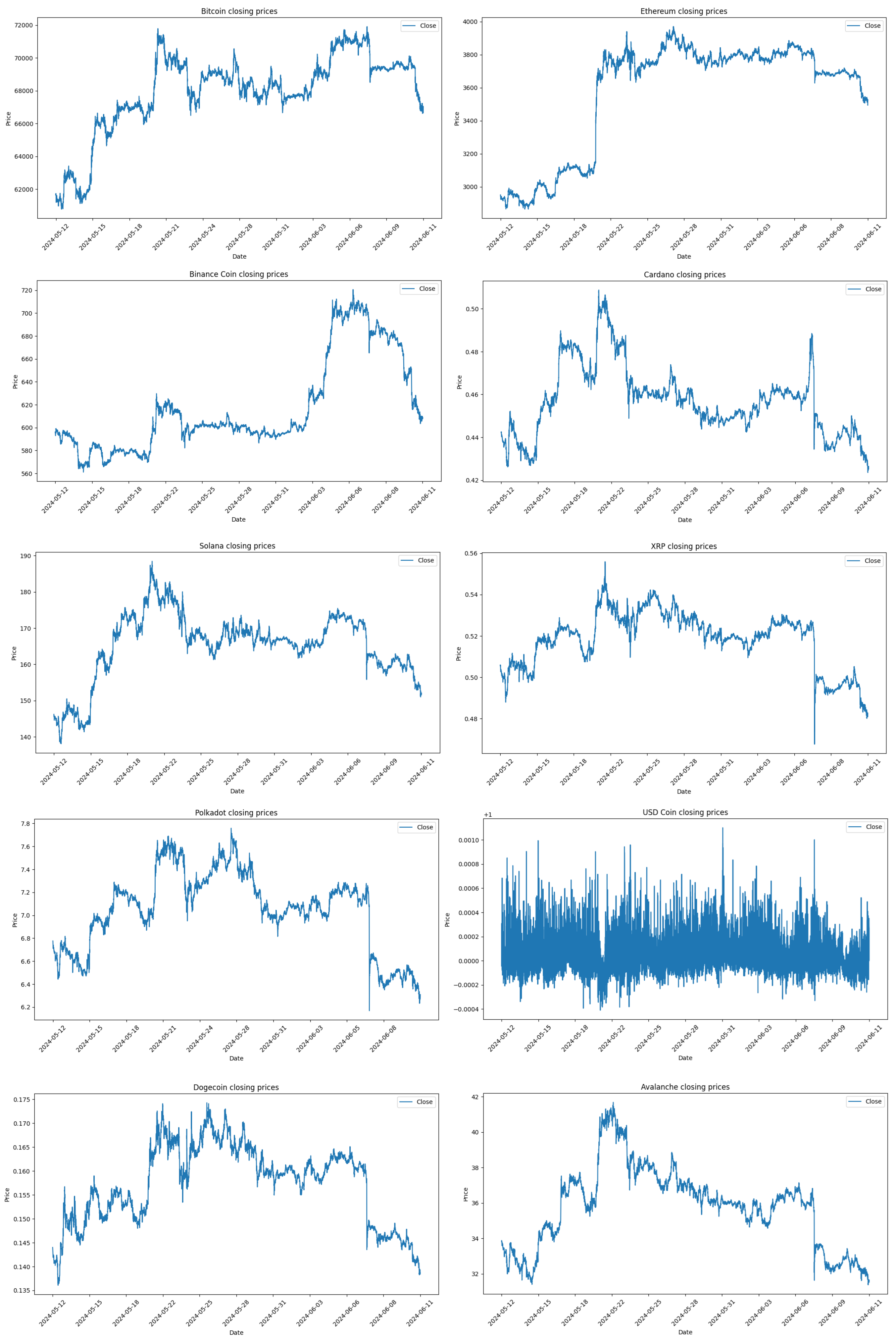Figure 7 displays the daily closing prices for Bitcoin (BTC), Ethereum (ETH), Binance Coin (BNB), Cardano (ADA), Solana (SOL), XRP, Polkadot (DOT), USD Coin (USDC), Dogecoin (DOGE), and Avalanche (AVAX) over the 30-day data collection period. Most cryptocurrencies, including BTC, ETH, BNB, ADA, SOL, XRP, DOT, DOGE, and AVAX, exhibit a general downward trend in their closing prices over this period. Cryptocurrencies like ADA, XRP, and AVAX show higher short-term volatility compared to BTC and ETH. Stablecoins like USDC stand out for their resilience during such market conditions. The figure highlights a challenging period for most cryptocurrencies with declining prices and varying levels of volatility.

3.2. Data Preprocessing

The data, obtained from the YFinance API, comprised minute-step price data for ten cryptocurrencies from 12 May 2024 to 11 June 2024. The dataset was initially examined for missing values; none were found. The Datetime attribute served as the index for the records, and its sorting guaranteed that the records remained sequential according to date and time. The Adj. Close column was eliminated from all cryptocurrency datasets due to its redundancy, as it includes equal values to the Close attribute.

A thorough examination was conducted for outliers using the interquartile range (IQR) method. Outliers were present and removed since they are likely to be due to market anomalies, which would affect the model performance. The removal of outliers did not significantly impact the dataset size.

To ensure data consistency across all cryptocurrencies and time periods, a series of checks was performed before data normalisation. These included verifying data alignment with other publicly available sources. Data consistency across different sources was confirmed before proceeding to data scaling.

While differencing is a common method for handling non-stationary time series, it was not employed in this study. Many GRU/LSTM implementations use normalisation techniques instead of differencing. This approach was chosen because the normalization method effectively handles data scaling issues without altering the inherent time series patterns. All features except the date and time were scaled using MinMaxScaler [14] to ensure consistent ranges (0–1) for all attributes across the different cryptocurrencies prior to applying the models. We selected this specific scaler because it effectively handles data with varying scales, thereby preventing features with larger values from dominating the learning process. This scaling was reversed during the model testing and validation phases.

Following data preprocessing, the dataset was then split for training, testing, and validation (80%, 10%, and 10%, respectively), with the last 60 data points reserved for validation, ensuring the models were thoroughly evaluated. This splitting strategy ensured that the model evaluation was based on unseen data.

3.3. Evaluation Metrics

After training the machine learning models, error metrics are calculated using the test dataset to evaluate the performance of regression models. The performance metrics measure how close the actual results are to the predicted values, with the most common ones being the mean absolute error (MAE), mean squared error (MSE), root mean squared error (RMSE), and mean absolute percentage error (MAPE) [15].

$$MSE={\displaystyle \frac{1}{n}}\sum _{i=1}^n\left(\right|y_i-{\hat{y}}_i{|}^2)$$

(1)

$$RMSE=\sqrt{{\displaystyle \frac{1}{n}}\sum _{i=1}^n\left(\right|y_i-{\hat{y}}_i{|}^2)}$$

(2)

$$MAE={\displaystyle \frac{1}{n}}\sum _{i=1}^n|y_i-{\hat{y}}_i|$$

(3)

$$MAPE={\displaystyle \frac{100}{n}}\sum _{i=1}^n{\displaystyle \frac{|y_i-{\hat{y}}_i|}{y_i}}$$

(4)

where $y_i$ represents the actual value, and ${\hat{y}}_i$ represents the value predicted by the model [16].

3.4. Models

First, we compare the performance of the eight different regression algorithms using the Bitcoin records for 60 min forecasts. This choice is due to the fact that Bitcoin is the most relevant and commonly used cryptocurrency in the analyzed studies. We selected the 60 min timeframe because it is the shortest time horizon under analysis, thereby ensuring optimal performance.

The comparative tests were based on the use of all attributes—Open, High, Low, Close, and Volume—as well as on just the Close attribute. The SARIMA model was only trained and tested using the Close attribute because it has some particularities that distinguish it from the other models, which will be explained next.

In general, the models can be used with data from different time intervals. The records are available through the YFinance API, which allows downloading records by the minute, hour, or day. For minute-level data, the last 30 days of data can be retrieved. For hourly intervals, data from the last 365 days can be retrieved, and for daily records, there are no restrictions. The decision to use minute-level data allows for a much larger amount of records for model training. Some models, such as neural networks, require a large amount of data to achieve better performance. In 30 days, there can be up to 43,200 records, while in one year of hourly data, there can be up to 8760 records, and in five years of daily records, there could only be up to 1825 records. Another relevant aspect of minute-step records is that the variation in values between records is less significant, which also helps to make predictions more accurate. Except for the SARIMA model, where values are trained minute by minute, for all the other models, there is a function to create forecasts in 60 min sequences, also known as sliding windows. This function is adjusted according to the forecast time horizon. Thus, the last 60 min are used to predict the next 60 min.

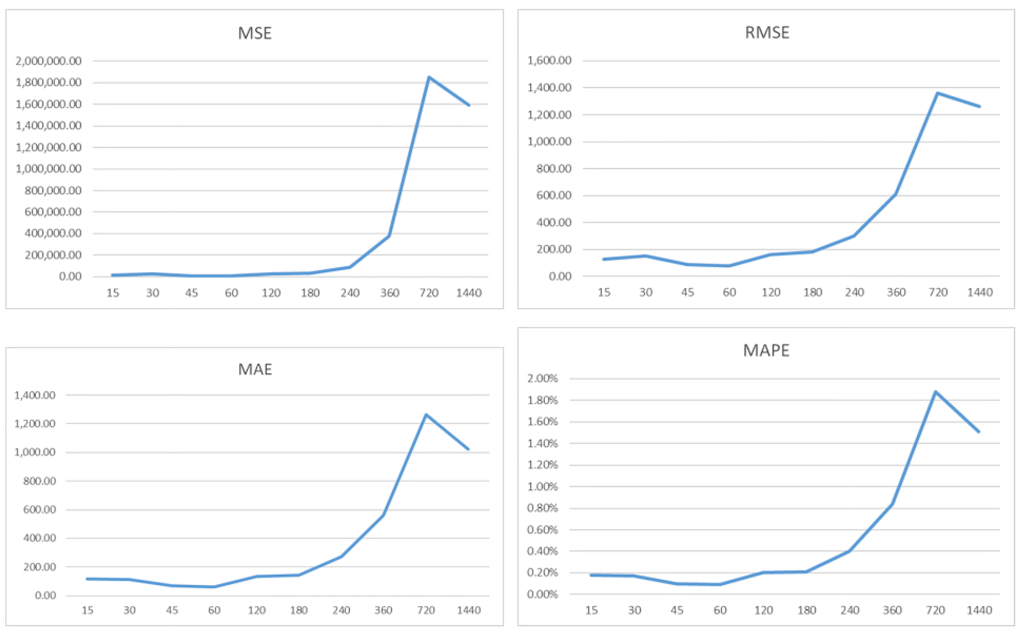
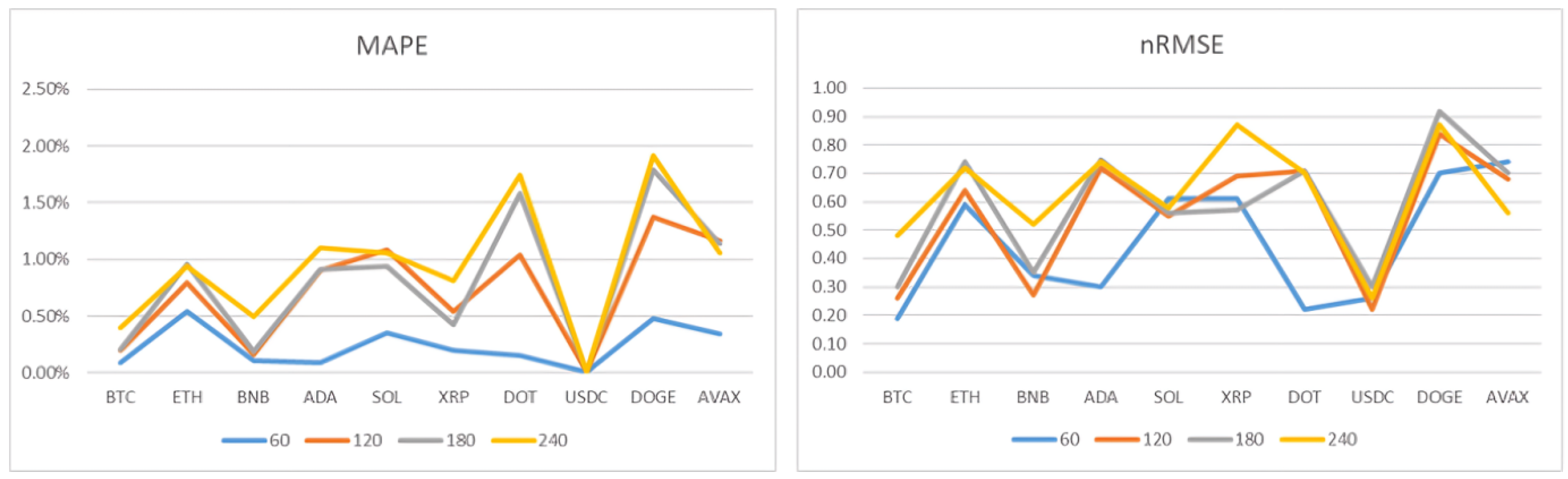
The model’s performance is measured using the metrics previously mentioned: MSE, RMSE, MAE, and MAPE. Additionally, the nRMSE metric is introduced, which corresponds to the RMSE metric but is obtained from normalized values, allowing for a better comparison of model performance across different cryptocurrencies, as each one has different magnitude values.

From the Keras library of the TensorFlow API, long short-term memory (LSTM) [17] and gated recurrent unit (GRU) [18] models were trained and evaluated using a grid search to identify the optimal hyperparameters. A 5-fold cross-validation was employed. The hyperparameters considered included the number of neurons (30, 50, 75, 100) and the number of layers (1, 2, 3) with the Adam optimizer. Model performance was evaluated using MAE, RMSE, and MAPE. Based on the results obtained, an architecture of 50 neurons and 2 layers was selected for both LSTM and GRU models, as it provided the best balance between model performance and computational cost. However, for computational reasons (limited resources: Intel i7 12650H 2.30 GHz processor, 16 GB RAM, NVIDIA GeForce RTX 3080 graphics card, from Taipei, Taiwan), a comprehensive hyperparameter search was not feasible for all models. For the remaining models (ARIMA, etc.), the default parameters were employed, providing reasonable baselines against which to compare the performance of the optimized LSTM and GRU models. This approach allowed for a focused analysis of the performance differences between the various model types while managing computational constraints.

The auto-regressive integrated moving average (ARIMA) [19] model is obtained through the Statsmodels library. The model used is actually SARIMAX, which is used to prepare seasonality and exogenous variables in the ARIMA model, but in this case, there are no exogenous variables in the data obtained, and for that reason, the model is referred to as SARIMA, and not ARIMA or SARIMAX. This model is very resource-intensive, and on the machine where it was tested, it was not even possible to load the entire dataset to train the model. Therefore, subsets of the records were loaded, and the point where the best results were achieved was with only 360 records, meaning the price of the last 360 min. Even so, the model takes a long time to train, which makes it impractical for deployment in an application, as it needs to be retrained with new data to make predictions, unlike the other models that can be saved and reused to make predictions with new data without requiring training the model again.

Linear regression (LR) [20] is the simplest regression model, and despite its simplicity, its performance was quite interesting. The previous model was observed to more or less follow the price trends but did not predict the major peaks in value variation. LR tends to be even more of a straight line when presented graphically. The main advantage is that it is a very simple and fast model to train.

The Random Forest [21] model is not very common for time series forecasting, and the training process is also quite heavy when used with a large amount of data. To avoid overloading the training process too much, a model with 100 decision trees was applied. The performance of this model was slightly worse than the previous models.

The support vector machine (SVM) [22] model, support vector regressor for regression problems, was tested with the kernel parameter set to RBF. This model is also heavy to train with large datasets, but it performs well, especially when trained with all attributes.

The XGBoost [23] model, in terms of training, is quite fast; however, its performance in validation fell well short of the previous models, especially when trained with all attributes. In the parameters, 100 decision trees, or predictors, were used, along with a learning rate of 0.1.

Lastly, LightGBM [24], a model derived from XGBoost [23], achieves better results with faster training. Using default configuration values, its performance, although not as good as neural networks, is better than XGBoost when used with all predictor attributes, but worse when used with only the closing price.

3.4.1. Analysis of Models Performance

Table 3. Models performance on a 60-min forecast of Bitcoin price.

	MSE	RMSE	MAE	MAPE	nRMSE
Using all attributes
LSTM	8163.73	90.35	71.87	0.11%	0.22
GRU	5954.89	77.17	60.20	0.09%	0.19
SARIMA	-	-	-	-	-
Lin. Reg.	6979.26	83.54	64.36	0.10%	0.20
RF	387,460.75	622.46	572.41	85.55%	1.50
SVM	10,301.07	101.49	83.40	0.12%	0.24
XGBoost	420,6051.13	2050.87	1053.07	1.57%	4.95
LightGBM	29,859.99	172.80	137.39	0.21%	0.42
Using just the Close attribute
LSTM	7237.85	85.08	67.87	0.10%	0.21
GRU	9307.22	96.47	75.98	0.11%	0.23
SARIMA	19476.59	139.56	114.16	0.16%	0.23
Lin. Reg.	6722.40	81.99	62.49	0.09%	0.20
RF	38281.06	195.66	167.82	25.09%	0.47
SVM	121987.11	349.27	338.49	0.51%	0.84
XGBoost	37715.50	194.20	148.61	0.22%	0.47
LightGBM	38132.43	195.28	165.60	0.25%	0.47

presents the performance of eight machine learning models developed for predicting Bitcoin prices over a 60-min horizon, with the gated recurrent unit (GRU) model emerging as the top performer across all metrics.

In contrast, models like SARIMA, while suitable for stationary time series, may struggle with the non-stationary nature of cryptocurrency price data, leading to lower prediction accuracy. The LR model demonstrated surprisingly strong performance, indicating the presence of some underlying linear trends in the data. The model’s RMSE of 83.54 and MAPE of 0.10% show the extent of this linear behavior. Although LSTM also demonstrates reasonable accuracy, its greater computational complexity, relative to GRU, does not compensate. The significantly worse performance of ensemble methods (XGBoost, LightGBM) underscores the limitations of traditional and ensemble methods in handling the high volatility and intricate dynamics of cryptocurrency prices.

The GRU model was rigorously evaluated by comparison with the second most efficient model, the LR model. We use MAE as the primary metric for statistically comparing both models because MAE is a more reliable way to measure the overall performance of cryptocurrency data, which can sometimes have huge price changes. MAE is more robust to outliers than MSE or RMSE, is easy to interpret, provides a clear understanding of the model’s typical prediction error, and focuses on the magnitude of the errors, which is directly relevant to assessing the practical usefulness of the model for investment decisions.

We performed two statistical tests on the MAE values obtained from the GRU and LR models applied to the last hour of 10 days in the period 1/09/2024 to 10/09/2024, as presented in

Table 4. Model comparison—MAE values.

	01/09	02/09	03/09	04/09	05/09	06/09	07/09	08/09	09/09	10/09
GRU	40.03	30.23	112.78	47.46	262.22	289.99	67.93	480.49	97.67	66.63
LR	42.66	35.23	138.41	49.88	268.38	295.91	69.90	488.42	99.29	69.95

.

To assess the statistical significance of the GRU model’s superior performance compared to linear regression, the normality assumption was first checked using the Shapiro–Wilk test on the differences in MAE between the two models. The Shapiro–Wilk test yielded a p-value of 0.000144, which is less than the significance level of $\alpha =0.05$, indicating a violation of the normality assumption. Therefore, the non-parametric Wilcoxon signed-rank test was used. The Wilcoxon signed-rank test resulted in a p-value of 0.00195, which is less than $\alpha =0.05$. We conclude that the MAE of the GRU model was significantly lower than that of the linear regression model (p < 0.001), confirming the superiority of the GRU model.

The GRU model’s superior performance can be attributed to several factors. First, the GRU architecture is particularly well-suited for handling sequential data, such as time series, due to its ability to capture long-term dependencies. This capability is crucial in cryptocurrency markets, where price fluctuations often exhibit complex patterns and temporal correlations. Second, the simplified architecture of the GRU, compared to LSTM, allows for faster training times without compromising accuracy. Third, the optimized hyperparameters identified during our grid search further enhanced the GRU’s performance. This careful optimization ensured that the GRU could effectively model both short-term and long-term patterns in the data.

In conclusion, the GRU model is not only the most accurate model tested but also the most practical for deployment in real-time forecasting systems, where computational efficiency is critical. Its performance highlights the potential for deep learning models to provide accurate, short-term predictions in highly volatile markets like cryptocurrencies.

3.4.2. Time Horizons

It is observed that the performance significantly decreases as the forecast horizon increases when using high-frequency data, which was expected, as forecasting so many steps ahead is much more difficult. Especially when the model is unable to predict major drops or peaks in value and cannot foresee changes in trend direction. In other words, if a cryptocurrency is in an upward trend, the model will make predictions in the same direction, and if there is a change in the trend, the model will not predict it, as there are no predictor attributes indicating such a change might occur.

In order to study the performance of the GRU network across different forecast time horizons, the GRU was configured to run up to 50 learning cycles (epochs); however, with the EarlyStopping method configured to tolerate 5 epochs if the loss function values start increasing, the process generally does not exceed 20 cycles in each training process.

Initially, shorter forecast horizons of 30 and 45 min were planned, but the performance did not improve enough to justify making them available in the web application. Longer horizons of 6, 12, and 24 h were also considered, but here, the performance dropped too much. Most likely, for these longer forecast horizons, the models would train better with hourly data instead of minute-level data.

The model’s performance was compared across all time horizons for Bitcoin, and as can be seen in Figure 8 and

Table 5. GRU model performance for different forecasting horizons.

Min.	30	45	60	120	180	240	360	720	1440
MSE	23,634	7786	955	25,713	33,575	89,106	375,233	1,854,184	1,589,417
RMSE	153.73	88.24	77.17	160.35	183.23	298.51	612.56	1361.68	1260.72
MAE	113.55	69.99	60.20	135.11	141.82	270.26	561.15	1264.40	1024.31
MAPE	0.17%	0.10%	0.09%	0.20%	0.21%	0.40%	0.84%	1.88%	1.51%
nRMSE	0.37	0.21	0.19	0.26	0.30	0.48	0.62	0.73	0.36

, the performance metric values remain stable up to the 240 min forecast. However, when extended to 1440 min, these values increase considerably.

4. Results Discussion

The GRU neural network, recognized as the most effective prediction method, was used to develop forecasting models for all selected cryptocurrencies throughout time horizons ranging from 60 to 240 min.

In terms of performance comparison between the different cryptocurrencies with varying magnitudes, the only comparable metrics are MAPE, which is a percentage metric, and nRMSE, which is a normalized RMSE value. As can be seen from Figure 9 and

Table 6. MAPE and nRMSE values of the GRU model for all cryptocurrencies.

	MAPE				nRMSE
Cripto	60	120	180	240	60	120	180	240
BTC	0.09%	0.20%	0.21%	0.40%	0.19	0.26	0.30	0.48
ETH	0.54%	0.79%	0.96%	0.94%	0.59	0.64	0.74	0.72
BNB	0.11%	0.16%	0.19%	0.50%	0.34	0.27	0.35	0.52
ADA	0.09%	0.90%	0.91%	1.10%	0.30	0.72	0.75	0.74
SOL	0.35%	1.08%	0.94%	1.06%	0.61	0.55	0.56	0.58
XRP	0.20%	0.54%	0.42%	0.81%	0.61	0.69	0.57	0.87
DOT	0.15%	1.04%	1.58%	1.74%	0.22	0.71	0.71	0.70
USDC	0.01%	0.01%	0.01%	0.01%	0.26	0.22	0.30	0.26
DOGE	0.48%	1.37%	1.79%	1.91%	0.70	0.84	0.92	0.87
AVAX	0.34%	1.16%	1.14%	1.06%	0.74	0.68	0.70	0.56

, an overall increase in forecast error values is observed from the 60-min prediction to bigger time horizons, with the exception of USD Coin, which has such subtle price variations and shows little difference across forecasts with different time horizons.

Except for USD Coin, the following observations stand out from the tests performed: Bitcoin achieved the best performance in terms of nRMSE across all four time horizons. Also, in terms of the nRMSE metric, the worst performances were with Avalanche at 60 min and with Dogecoin at 120, 180, and 240 min, along with XRP in the last case. In terms of MAPE values, Bitcoin and Cardano had the best performance at 60 min, Binance Coin at 120 and 180 min, and Bitcoin again at 240 min. The Ethereum forecast had the worst MAPE values at 60 min, followed by Dogecoin at 120, 180, and 240 min.

Table 7. Performance comparison to related work.

Ref.	Cripto	Forecast	RMSE	MAPE	MAE	MSE
[4]	Bitcoin	Price in 21 days	251.61	0.31%	164.49	63,307.31
[25]	Bitcoin	Daily price	458.02	-	345,512	209,778.00
[8]	Bitcoin	Daily price	217.53	3.26%	79.25	-
[10]	Bitcoin	Daily price	0.01	0.01%	0.01	-
[26]	Bitcoin	Daily price	7527.30	0.16%	6631.80	-
[27]	Bitcoin	Daily price	-	2.42%	0.00	1.41
[28]	Bitcoin	Daily price	0.07	0.03%	-	-
[29]	Bitcoin	Daily price	1987.11	0.18%	-	-
[30]	Bitcoin	Daily price	1447.65	0.03%	-	-
[31]	Bitcoin	Daily price	3599.17	-	-	2139.91
[32]	Bitcoin	Daily price	-	0.07%	-	0.04
[33]	Bitcoin	Daily price	1469.41	-	-	2,159,166.25
[13]	Bitcoin	Daily price	372.84	-	-	-
[34]	Bitcoin	5 min price	1.44	-	-	-
[35]	Bitcoin	3 months price	673.00	-	-	-
[36]	Bitcoin	Daily price	5251.20	-	-	-
[37]	Bitcoin	Daily price	6720.14	-	-	-
[38]	Bitcoin	Daily price	367.00	-	-	-
[16]	Bitcoin	Daily price	-	0.14%	-	-
[6]	Bitcoin	Daily price	-	1.56%	-	-
[39]	Bitcoin	Daily price	-	1.69%	-	-
[40]	Bitcoin	10 days price	-	-	83.27	-
[41]	Bitcoin	Daily price	-	-	0.02	-
[42]	Bitcoin	Daily price	-	-	0.02	-
[43]	Bitcoin	1 month price	-	-	-	271.00
[44]	Ethereum	Daily price	253.68	-	115.91	64,355.56
[45]	Litecoin	Daily price	0.01	-	0.00	0.00
[46]	Ethereum	Daily price	-	0.75%	-	-
[47]	Cardano	Daily price	0.60	-	-	-

offers a comparison of performance metrics from several related works in the field of cryptocurrency price forecasting. While it is not possible to make direct comparisons due to the diversity in datasets, forecast horizons, and machine learning models used, we can draw several important conclusions from this table that highlight the uniqueness and strengths of our approach.

This study’s GRU-based approach, uniquely tailored for minute-level data, excels in short-term predictions within the highly volatile cryptocurrency market—a context less explored in prior research. While the GRU model inherently handles non-stationary time series, the inherent unpredictability of cryptocurrency prices remains a challenge. To mitigate the impact of abrupt market shifts, we utilized a recent 30-day dataset, focusing on relatively stable, short-term patterns.

Unlike many studies focused on daily or multi-day forecasts, our results demonstrate the GRU’s superior performance over traditional models (ARIMA, Random Forest) for minute-level predictions, achieving lower RMSE, MAE, and MAPE values. Furthermore, our study extends beyond Bitcoin, proving the scalability of the GRU-based system across multiple cryptocurrencies within a broader financial context.

These findings highlight both the novelty and value of our work, addressing a gap in the literature by tackling high-frequency forecasting challenges. This study contributes to the field of cryptocurrency forecasting, particularly for real-time applications, by demonstrating the effectiveness and scalability of a GRU-based approach in capturing short-term price dynamics.

5. Deployment

The cryptocurrency price forecasting system is deployed as a user-friendly web application, accessible at https://crypto-mm.streamlit.app/ (accessed on 4 April 2025). The application leverages a trained GRU model and retrieves minute-step data from the YFinance API to generate predictions for 1, 2, 3, and 4-hour horizons. A key feature is the ability for users to trigger model retraining, allowing the system to adapt to shifting market conditions. The data are loaded onto the server, where all the processing is also performed. In terms of functionality, the system can be divided into three modules (Figure 10).

Data—In this first module, the application uses the YFinance API to transfer minute step data from the last 30 days to the application and then saves them in a CSV file. The application allows the loading and graphical visualization of this data.

Models—The models can be retrained, which can be beneficial for performance, as data patterns may change over time, as previously mentioned, see Figure 11. However, retraining the models is not mandatory to make new forecasts because there is an independent model for each cryptocurrency and for each forecast horizon. Once the models are trained, they are stored to be used later when new forecasts are made.

Forecasts—This module executes the forecasts for the selected cryptocurrency and time horizon, displaying the predicted future price trend.

The application is hosted on a secure Amazon Web Services (AWS) EC2 t3.large instance (2 vCPUs, 8 GB RAM, 100 GB SSD storage, Ubuntu 22.04 LTS). This configuration balances cost-effectiveness and processing power. While the current infrastructure is sufficient, significant increases in user traffic or model complexity could necessitate future infrastructure upgrades, which will be closely monitored.

Robust security measures to protect user data and application integrity are inherent to the application due to its development using Streamlit (vs. 1.20.) and its deployment through GitHub (vs. 3.4.16). These include HTTPS encryption for data transmission, the use of firewalls and intrusion detection systems on the AWS server, and regular security audits. No personally identifiable information (PII) is collected because the application does not require user registration or authentication. However, to ensure continuous improvement and address potential issues, users are encouraged to provide feedback via email at crypto.mm.feedback@gmail.com.

6. Discussion and Limitations

The findings of this study have several significant practical implications for cryptocurrency investors and traders. The high accuracy achieved by the GRU model in forecasting short-term price movements (up to 4 h) allows for the development of more effective trading strategies. The real-time price prediction web application provides investors with an accessible tool for making more informed decisions, potentially mitigating risks and improving profit opportunities. Furthermore, the identified superior performance of the GRU model compared to other algorithms, such as LR, LSTM, and conventional machine learning models, offers valuable insights for future research and development in algorithmic trading systems.

The reliance on a 30-day dataset of minute-level data is a limitation of this study. While this timeframe allowed us to focus on high-frequency dynamics, it may not fully capture longer-term trends or structural market changes that could influence forecasting accuracy. To address this limitation, future research should validate the findings using longer datasets spanning several months or years. This would provide a more robust assessment of the model’s performance under various market conditions and its ability to adapt to evolving market dynamics. Furthermore, incorporating techniques for handling concept drift, where the statistical properties of the time series change over time, could improve the model’s long-term forecasting accuracy.

While this study primarily focuses on an empirical analysis of GRU performance in high-frequency cryptocurrency forecasting, it is important to acknowledge the limited theoretical advancements presented. Our findings align with the theoretical understanding of recurrent neural networks, particularly GRUs, in handling time-series data. GRUs are designed to capture temporal dependencies and learn complex patterns from sequential data, making them well-suited for forecasting in dynamic environments. Their gating mechanisms (reset and update gates) enable them to selectively remember or forget information from previous time steps, allowing them to adapt to evolving patterns and filter out irrelevant noise. This is particularly relevant in cryptocurrency markets, where prices are influenced by a multitude of factors and exhibit complex, non-linear dynamics. The GRU’s ability to capture these dependencies, while computationally efficient, is a key factor in its superior performance compared to other models. Future research could explore more theoretical aspects, such as analyzing the model’s learned representations or developing novel architectures specifically tailored for cryptocurrency forecasting.

7. Conclusions

This study presented a high-frequency cryptocurrency price forecasting system using various machine learning models, with a specific focus on short-term prediction horizons. After extensive experimentation, the gated recurrent unit (GRU) neural network was found to be the most effective model for predicting 60-min price movements across multiple cryptocurrencies. Compared to alternative approaches, including LSTM, ARIMA, and traditional regression models, GRU consistently delivered superior results, achieving the lowest error rates across several key metrics such as MSE, RMSE, MAE, and MAPE.

The high volatility and non-stationary nature of cryptocurrency prices make accurate forecasting a challenging task. Nevertheless, the results demonstrated that deep learning models, particularly GRU, are capable of effectively capturing complex patterns in minute-level data, making them well-suited for real-time applications. The integration of these models into a web application highlights the practical implications of this research, offering users the ability to generate real-time cryptocurrency forecasts across various time horizons.

Future research could explore several avenues to build upon this work. First, incorporating external data sources (financial news sentiment, macroeconomic indicators) could enhance predictive power. Second, expanding the forecast horizon to 6–12 h would provide further insights into longer-term predictability. Finally, while the GRU model performed best here, exploring transformer models or attention mechanisms, which have shown promise in other time series applications, could yield further improvements in cryptocurrency price prediction.