1. Introduction
Broadcast audio transmissions like Frequency Modulation (FM) or web radios carry different kinds of content like commercial music tracks, advertising spots, talk shows, news, etc. Within this context, being able to differentiate the nature of the audio being broadcast is crucial for commercial or reporting reasons such as monitoring, metadata, and royalties. Depending on national regulations, radio stations can be asked to produce periodic reports containing all the songs played within a requested time range, providing metadata such as the date and time when each song has been played or the duration.
To automate the process, there currently are systems able to automatically recognize what song is being played, which at least removes the necessity for a human operator. Such systems are usually based on extracting identifying features from the audio and matching them against a large pre-existing song database, and they have to work 24/7, wasting resources on non-music content [
1].
Automatic song identification technologies typically rely on “audio fingerprinting”, which is based on hashing unique landmarks or features of the signal and is designed to be robust to audio degradations (e.g., equalization, noise, etc.) and even handle pitch or tempo deviations [
2]. As an example, one of the most commercially famous solutions called Shazam (formerly Shazam Entertainment Ltd., now owned by Apple, Inc., Cupertino, CA, USA) [
3] is based on the identification of landmarks as peaks on the spectrogram, with the basic idea that the sequence of distinct time-frequency pairs is an identifier for a specific song. Once the audio has been fingerprinted it is then compared against a database using fast hash table lookups.
Other solutions employ more advanced or more diverse input features, with technologies that include the following [
2]:
Constellation maps which take into account relationships between fingerprints, thus also considering their sequential nature;
High-level musical features such as the tempo, chord progression or lyrics. The usage of such metadata implies the existence of high-level models able to infer data such as harmony or to recognize (sung) voice and convert it into text (lyrics);
Feature-based high-level Machine Learning, which may employ classifiers trained on acoustic features usually derived from the spectrum, cepstrum (MFCC) [
4] or pitch domain;
Deep Learning (DL) is usually implemented with Convolutional Neural Networks (CNNs) trained on spectrogram images, which automatically extract relevant features [
5].
Identifying specific songs is a task that current technologies such as Shazam handle relatively well, making them suitable for automating the tracking of songs played on radio broadcasts in order to count them and produce reports and statistics. However, this approach requires the identifier to operate continuously, 24/7, leading to numerous service calls. This remains true even during times when the radio station is not streaming music, such as during talk shows or advertisements. In these instances, the song identification service may be invoked unnecessarily, prompting interest in a preliminary method to differentiate between commercially played tracks and other content, such as ads, speech or non-music segments.
Incorporating such a discrimination system, which we will refer to as a “music vs. non-music” discrimination problem, helps reduce the inefficient use of resources for monitoring radio broadcasts, lowering operational costs.
As previously mentioned, the primary challenges in developing such systems stem from the presence of music in advertisements and background soundtracks during talk shows. The fragmented structure of talk shows, where pauses in speech allow the music to become more prominent, along with the variability in advertisements—some of which include jingles—further complicate the task.
The aim of this paper is to propose a system that distinguishes commercially played tracks (“music”) from everything else that is being broadcast (“non-music”) on radios, to be used as a preliminary filter for reducing service calls to song identifiers, in turn, used to automate the reporting process.
Currently, the problem of preliminarily identifying if a radio station is playing a commercial track can also be partially faced by relying on broadcast metadata. However, such a solution is not definitive or robust because it is unsuitable for AM and FM without RDS (Radio Data System), as well as smaller stations where metadata is not transmitted, and in general even with bigger stations there is a number of human annotation errors and gaps.
The ACRCloud SDK service (by Google LLC, Mountain View, CA, USA) includes a radio broadcast suite, which reports “Cover Song Identification” and “Audio Fingerprinting” as their main resources, and includes services like unidentified content detection and music-vs-speech classification [
6]. ACRCloud’s services are mainly directed towards song and custom content identification, self-reportedly based on fingerprinting technologies and, to the knowledge of the authors, with no alleged preliminary filter for avoiding unnecessary service calls: as stated by Mediarealm, “listens to your internet stream in real-time, detects the songs you are playing, and sends the song data through to a service” [
7]. Other notable services are Gracenote (Gracenote Inc., Emeryville, CA, USA) [
8], which specializes in the addition of contextual metadata and allows for easier discrimination if paired with SMD, and TuneSat (TuneSat LLC, New York, NY, USA) [
9], which distinguishes when a song is being used for plain commercial broadcast versus when it is part of an ad, and it is a royalty service based on fingerprinting.
Other automatic solutions employ some kind of Speech-Music Discrimination (SMD) algorithms to distinguish between music and human speech, which may then be enhanced by radio metadata (if available) or fingerprinting. In a seminal 1997 work, Raj et al. [
10] explore the effects of background music corrupting speech recognition, which reflects the problem in this paper, finding out that algorithms that have been successfully applied to noisy speech are also helpful in improving recognition for background music [
11].
Many more complex solutions nowadays employ some kind of Deep Learning (DL) systems, often based on Convolutional Neural Networks (CNNs). CNN systems are based on a backpropagation neural network architecture where each layer performs multidimensional convolution (filtering) instead of simple dot products, to the point that each “neuron” is actually a filter matrix, and its pivots are the learnable (weights) [
12]. This behavior makes CNNs very suitable for image analysis because its filtering nature allows the identification of graphically localized features within a pixel matrix, and its multi-layer architecture performs an automatic feature extraction. Therefore, when dealing with audio analysis, it is customary to transform the signals into an image file (pixel matrix) that holds useful characteristics of the sound, leading to spectrograms being a gold standard [
13]. Spectrogram CNN-based deep learning systems have become a standard in audio analysis for various applications, including industrial-grade voice analysis [
14], speaker recognition [
15] and music classification [
16].
As anticipated, most studies on the subject either focus on inter-song classification (by genre, cover identification, etc.) or music-vs-speech with no mention of ads or talk shows with background soundtracks.
A preliminary work from Wieser et al. [
17] used an MFCC+SVM pipeline to distinguish music from speech from radio podcasts, notably finding issues when songs had no clear harmonic context and featured mainly rhythmic elements. One of the considered approaches is the one using a CNN developed by Jang et al. [
18], using two public audio datasets featuring music, speech and noise samples: the “Mirex 2015 MuSpeak” [
19] and the GTZAN set [
20]. These samples have been mixed artificially in order to obtain three different combinations: music with speech, music with noise and speech with noise. The developed system reached accuracies spanning from 86.5% to 95.9%, but sources varied from CD tracks to internet videos, with little attention to the eventual presence of audio artifacts typical of radio transmissions (distortion, compression), and most notably, overlaps were made artificially without reflecting real talk shows or ads.
Another approach is based on the Temporal Convolutional Network (TCN) developed by Lemaire and Holzapfel [
21]. TCN is a recently developed technology based on a common Convolutional Neural Network, but it is also able to take into consideration temporal factors of data, so it is able to infer rhythmic elements. Different public audio datasets have been used to develop the proposed system: the MUSAN Corpus [
22], the GTZAN music dataset [
20], Scheirer–Slaney Music Speech Corpus [
23], Mirex 2015 MuSpeak [
19], OFAI Speech and Music Detection Dataset [
24] and ESC-50: Dataset for Environmental Sound Classification [
25]. Moreover, an ad hoc developed dataset featuring music, speech and noise samples has been used: the Sveriges Radio dataset [
21]. Both real broadcast samples and artificially generated samples mixing music, speech and noise have been used. Samples have been resampled to 22,050 Hz and split into 90 s-length files. Data augmentation has been used, with music and speech randomly overlapping in order to train the system on those cases deemed “borderline”. The developed system reached an accuracy of 96.8%.
The implementation by Tsipas et al. [
26] diverges from neural network-based methods, instead utilizing classical machine learning classifiers such as Support Vector Machines (SVMs), Random Forest and Logistic Regression on acoustic features representing temporal, spectral and cepstral characteristics. Although the maximum accuracy reaches 97.7%, the dataset is limited by being composed of under three hours of material composed speech and music samples artificially mixed to re-create “non-music” in broadcasts.
A recent study by Bhattacharjee et al. [
27] deals with the specific problem of music overlapped with speech and describes an interesting feature extraction pipeline yet again centered on the presence of percussive elements but has no direct implications with radio broadcasts.
The main difference between plain “music vs. speech” and “music vs. non-music” is that in most radio content, there actually is some kind of music background, be it a jingle in ads or background tracks in talk shows. Thus, different sources are overlapped, and the problem is redefined as contextual analysis, where the non-music bits have to be identified by the explicit or implicit identification of complex patterns such as the presence of speech (non-rhythmic and not sung voices), the more frequent changes in pace or sound, the pauses in speech, etc.
To the knowledge of the authors, there currently are no reliable, publicly available systems for preliminary filtering of the broadcasted content, which in turn allows greatly reduced service calls to identifier software, minimizing cost and net traffic.
With these premises, the authors anticipate that very system proposed and implemented within this work is currently being employed in the Italian industry with success, embedded in the solution called “Compilerò X Radio” [
28] by DaVinci Solutions S.r.l., offering an automatic music report generation system for Italian radios and web-radios compatible with the requirements of Italian royalties collecting authorities like SIAE [
29], SCF [
30] and LEA [
31,
32].
As far as technology goes, in line with the previously mentioned studies, we decided to implement our solution with a custom Convolutional Neural Network (CNN) applied to spectrogram images. A common criticality with the existing literature is related to the datasets used, which often only employ music or speech that the authors try to mix or do not come from real radio broadcasts.
With the aim of building a reliable, case-specific dataset without having to rely on artificial data generation or excessive augmentation, we strive to collect audio from real radio broadcasts from various stations and thus employ our custom dataset made of 139 h of audio containing music and “non-music”.
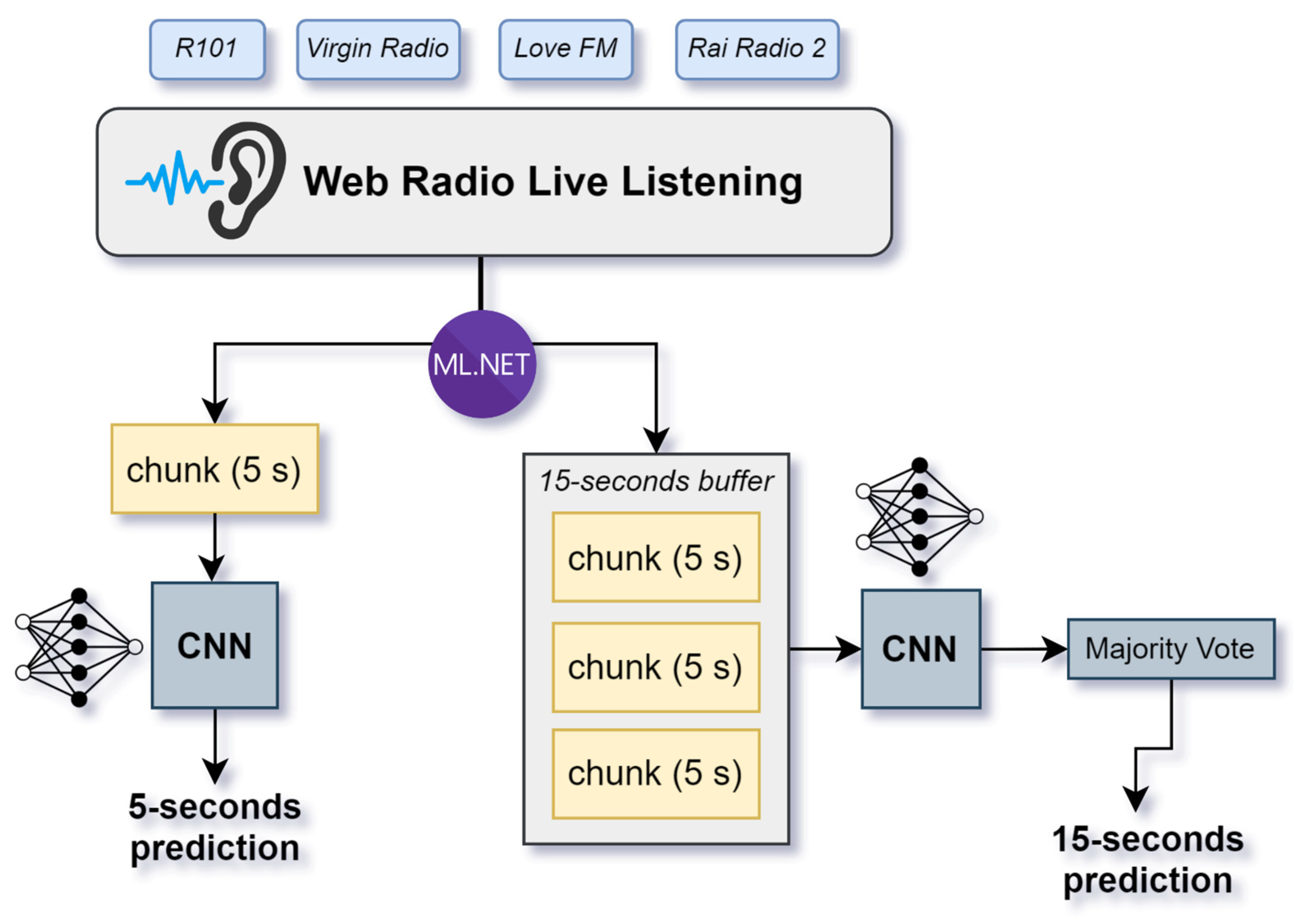
The developed system is based on a custom architecture CNN trained on spectrograms with the aim of distinguishing “music” as in commercially played tracks versus “non-music” as in everything else, including speech, talk shows or ads. The system has to work in a robust way and with a fast inference because its use case requires it to be able to discriminate audio content on 15 s length samples in order to decide whether to make service calls to song identifiers. In our case, the 15 s sample is split into three 5 s chunks, and the final prediction is based on the most recurrent prediction among the three. Additional experimentations have been carried out and presented regarding the usage of data augmentation and radio-like pre-processing on the raw audio data.
2. Materials and Methods
2.1. Dataset
The dataset was developed specifically for the subject of this paper and consists of audio from radio broadcasts mined from internet streams. It has been developed following a partnership with an Italian local FM radio named Love FM [
33], which granted access to its broadcast database. Part of the dataset was also developed by recording other famous Italian FM radios, with Rai Radio 2 [
34] used as an additional source for training samples and two other radios only used in the test set (Virgin Radio [
35], R101 [
36]) to check the performances of the models on material coming from previously unseen radio broadcasts.
More than 300 h of the broadcast were recorded and stored, but not all of them were used as training/testing material because we wanted to avoid the usage of “consecutive” chunks coming from the same source, which could bias the training set or, especially, the testing performances if chunks from the same source appeared in both training and test set. All recordings were manually annotated and classified into two classes: music and non-music. In general, the music class only contains commercially played tracks, whereas non-music entails everything else, including speech or ads. As for mixed content, it was classified according to the predominant source both volume and context-wise. As an example, a talk show where a speaker talks over some background music is classified as non-music as the predominant part is the speaker’s voice.
A borderline case is represented by all-music jingles. Although they do not represent commercially sold music tracks, they ultimately can be considered original songs, and their structure and sound are identical to them. Therefore, they have to be considered as “music”, also taking into account the fact that they would be impossible to classify otherwise for a model trained to distinguish pure music from other elements.
All samples were ultimately recorded in the .wav PCM format with a 44,100 Hz sampling frequency and a bit-depth of 16 bits, but the nature of the sources was various and each different radio sounded different. In order to equalize the dataset, a pre-processing pipeline was applied.
Moreover, because radio broadcasting usually involves additional processing when sending data over FM instead of web radios, a radio preset was also applied in order to check the performances of the models.
All the audio material will then be converted into mel-spectrograms, so the final dataset will be made only by spectrogram images, keeping the 2 subsets classification in music and non-music. The 2 subsets will be made of the same number of samples in order to have a balanced trained model.
Finally, as a benchmark, we also evaluated our system on the GTZAN dataset, which contains 1000 music tracks of 30 s in length each [
20].
2.2. Pre-Processing
All the audio material has been cut into 5 s length samples with a sample rate of 44,100 Hz and a bit-depth of 16 bits, storing them in the non-compressed WAV PCM format.
Having a huge amount of source material, it has been possible to generate 5 s length samples randomly selecting different parts of the audio in order to have non-continuous sequences that could end up creating biases. In the end, a grand total of 100,000 non-consecutive broadcast chunks were used in the training set, for a total of roughly 139 h of audio material.
Audio samples are stored after formatting and pre-processing with the following specifications:
Non-compressed WAV PCM format;
Mono channel;
Original sample rate: 44,100 Hz, then reduced to 22,050 Hz by decimation;
Bit-depth: 16 bit;
Fade-in and fade-out made with rapid volume envelopes of 0.5 s at the beginning and at the end of the sample, resulting in a windowing process used to remove any possible artifacts introduced by the cutting process.
Because different radio stations provided audio with different wide bands, we opted to reduce everything to the 20–11,025 Hz band. This was done by decimation (downsampling with an anti-aliasing low-pass filter) by simply reducing the original sampling rate, which has the added advantage of reducing file size as well as the amount of information for the CNN.
Acoustic information above 11 kHz is less critical for distinguishing between songs and non-music segments. This is because speech typically contains much less significant information beyond 8 kHz [
37], whereas musical elements often do [
38]. Consequently, audio segments categorized as “non-music” and consisting solely of speech remain clearly distinguishable from music due to the lack of relevant spectral information above 8 kHz. However, when background jingles are present, high-frequency information becomes less relevant compared with detecting overlapping voices and analyzing rhythmic elements, whose transient features reside predominantly in lower-frequency bands [
38].
This pre-processing is applied indiscriminately to all samples entering our models in the training, test or inference phase.
Differently from web stations, in radio broadcasting, especially in the FM industry, it is customary to process audio in order to reduce the dynamic range and reach a very high loudness. This processing was usually carried out by using heavy compressors, limiters or stereo image controllers, and is now also implemented digitally [
39]. Of course, this is a destructive process for the audio and creates noticeable differences in volume, dynamic range and even equalization because it inherently creates distortion. Therefore, we chose to also experiment by introducing this processing to our dataset in order to check if performances would reduce the inputs taken by FM radio and to check the robustness of the models. In order to process audios with a real radio broadcast pipeline, we used a digital preset provided by Love FM radio and used in their own broadcast, relying on a software named Thimeo Stereo Tool (v10.10) [
40]. The preset includes the following audio processing chain:
Heavy multi-band compression in order to reduce dynamic and get a very high loudness;
Equalization that emphasizes low, mid-low and high frequencies and reduces the presence of mid-high frequencies (roughly between 800 and 5000 Hz);
Hard-limiting to 0 dB, avoiding any clipping;
Stereo widening. This is applied before converting audio to mono by simple channel averaging. Stereo wideners work by manipulating the phase, timing, or EQ differences between the left and right channels to create a sense of wider stereo imaging, and in general, this may bring to more phase cancellation between the channels, resulting in a less rich, duller-sounding mono signal.
For consistency, models trained on processed versions of the dataset will also make inferences on audios that endured the same processing pipeline.
In order to transform audio into images suitable for CNN training, we opted to use mel-spectrograms [
41]. Differently from “classical” spectrograms, they are generated using the Mel scale, which is a spectral re-weighing whose main aim is to reproduce the human sound perception, which is not linear across the whole spectrum. Due to this behavior, it is one of the most used solutions for Machine Learning applications [
42], and it follows this formula:
Spectrograms were generated from 5 s chunks and were saved as square images with a resolution of 256 × 256 pixels. Square images are chosen because of the filtering nature of the 2D convolutional layers of the CNN, which then require no padding.
Mel spectrograms are generated with the following characteristics:
Sample rate of 44,100 Hz, same as the source audios;
FFT size of 8192 in order to have a high-quality representation of the audio;
FFT step size of 828, whose value influences the image width;
FFT bin count of 256, whose value is equal to the image height;
Maximum frequency of 11,025 Hz, same as the input bandpass filtering;
Color scale set to grayscale, in order to simplify work for the CNN [
43] by generating a 1-channel input.
Figure 1 details some Mel-spectrogram examples used for the CNN training.
2.5. CNN Architecture
We implemented custom CNN models trained on grayscale, 256 × 256-pixel mel-spectrogram images. We experimented with several architectures, changing the number of hidden layers and neurons/filters, using shallower or deeper nets. We also experimented by using pre-trained CNN structures, namely the ResNet50 [
48] pre-trained on the ImageNet dataset, which has already been proven effective in audio analysis. However, after several attempts, a custom architecture was chosen, as it was the best performing on experimental subsets and was subsequently used in all the different training scenarios of the present paper. Many different models were trained on the same architecture in order to better assess performances and generalization power over different variations of datasets: reduced, radio-processed and extended.
The CNN has been developed using the Tensorflow framework [
49] and the custom architecture is described in
Figure 3 with a flowchart.
The network architecture consists of a repeated sequence of three layers, applied four times, with the only variation being the filter size parameter in each repetition. The final three layers are responsible for flattening the data and reducing them to the target number of output classes, which in this case is two. A Conv2D layer applies convolution with ReLu activation to extract features, followed by BatchNormalization for stability and MaxPooling2D to downsample. The Flatten layer converts data into a 1D array for Dense layers, which perform classification with the final output layer.
An 80-20 training-test split has been performed so that each model was evaluated on 20% of the initial training set. As mentioned earlier, trained models were then re-evaluated on external validation data gathered from other radio stations.
Tensorflow checkpoints are used in order to save only the model with the highest accuracy regardless of the reached epoch iteration number, and they have been configured to store the model only if its accuracy is higher than 90%. A stopping criterion over the epoch iterations was set in order to stop training after reaching max accuracy on the test set without improvements over the next 5 epochs. The authors anticipate that no checkpoint/stop was reached after the 50th epoch.
The net was trained with 64-sample mini-batches, chosen as a compromise between a reasonably high number of samples for a more comprehensive gradient and the fact that, with hundreds of thousands of data, there is enough room for iterations and generalization. We used an adaptive learning rate Adam optimizer [
50] over an initial learning rate of 0.001, with rates for each parameter being computed using the first and second moments of the backpropagation gradients:
where
’ represent the new learnable set for the network, updated from
with an adaptive learning rate of
scaled by the momentums
and
;
is an arbitrarily small value. The momentums
and
refer to the first and second moment of the gradient (computed using the Hadamard product [
51] of the gradient of the loss function), normalized by the beta values to the power of the iteration.
The learning rate adapts following two hyperparameters
b1 and
b2, usually initialized as values close to 1 (like 0.99) and raised to the power of the iteration:
where
t is the
t-th iteration.
3. Results
Three different models of the selected CNN architecture were trained on different versions of the dataset: the first one involves 70,000 initial samples, a 10× data augmentation that leads to 700,000 samples and applies the previously mentioned broadcast pre-processing to the same dataset. The second one features the same dataset and augmentation but without additional processing. The last one employs an extended version of the dataset, for a total of 100,000 initial samples and a 7× data augmentation (leading to 700,000) to check the importance of the data augmentation and of the ratio between augmented and non-augmented.
The statistical analysis brought an MMD of 0.0142 for the comparison of the distribution of the augmented vs. original dataset, which suggests similarity between the two sets. All intermediate possibilities (less/more augmentation, applying broadcast processing to the extended dataset, etc.) were tried as well but did not lead to noticeable results in terms of accuracy increase or decrease. Training results and a synopsis of the models are reported in
Table 1.
The training accuracy value is the value returned by Tensorflow at the end of the epoch, and it is not the accuracy of a real-world scenario, which will be calculated by testing these models against live, real radio recordings.
As for validation, we used the inference system we described in the “Inference” section live on web radio streaming, which resulted in newly acquired audio samples from four radios: Love FM, Rai Radio 2, Virgin Radio and R101.
Only the first two radios provided samples used in the training set, whereas Virgin and R101 were previously unseen by the models. A total of 1360 samples, i.e., 2 h of validation audio, were gathered by our live test and were annotated by human operators with the following criteria that mirror those used in the training dataset:
Every bit of a commercially played music track is considered “music”;
Music-only jingles, which ultimately consist of an “original” song (albeit commercial), are also considered “music”;
Talk shows with background music are considered “non-music”;
Ads with slogans, pre-recorded voices or non-musical elements are considered “non-music” regardless of the background;
Speech-only, or noise, are considered “non-music” for obvious reasons.
Inference model used (broadcast processing, no-broadcast, extended);
Radio (Love FM, Rai Radio 2, Virgin, R101);
Aggregated 5 s or 15 s input. In the latter case, the final accuracy refers to predictions obtained by majority voting between the three consecutive 5 s chunks of predictions.
Validation results are reported in
Table 2,
Table 3,
Table 4,
Table 5,
Table 6 and
Table 7 and contain the results of our models applied on new recordings of stations that were included in the training set, as well as new datasets recorded from new radio stations, namely R101 and Virgin (with different schedules and audio pre-processing).
Table 8 reports the results on the GTZAN dataset for the task of detecting music, with the same division into genres originally featured in the dataset metadata. Because all samples in GTZAN are music, the best possible scenario was obtaining 100% accuracy in its detection, which was achieved on 15 s buffers.
4. Discussion
With the aim to build a solid pipeline and train on real-world data with no artificial audios and with the right dimensionality, we collected 139 h of non-consecutive audio chunks from two radio broadcasts, trained a custom CNN architecture and validated it with a custom system running live on web radios.
In the literature, there is a certain scarcity of examples of automatic systems that detect music or non-music from radio broadcasts. Although some studies report promising performances, their criticality lies in the dataset, which is often too small or synthetic, built by manually adding background to speech data. However, the “non-music” data built this way do not reflect what is usually broadcast on radio stations, which includes peculiar covariates such as professionally recorded and compressed speech uttered by voice professionals in a controlled environment, mixed with background music and/or sound effects, and ultimately processed for broadcasting.
Table 9 displays a brief comparison of studies alongside ours.
Three main versions of the CNN were trained in order to explore different aspects: the first one is on a reduced dataset (70,000 samples) whose number is increased by a 10× data augmentation. The second one employs radio-like processing that features heavy compression and similar artifacts, made using a real radio preset: this net was used in order to check if our systems would still work were they to be applied on FM radios where audio is processed. The third net uses more training data and less augmented ones.
Before dealing with the results, some considerations are due regarding the input data: as anticipated, we strive to collect many real-world, uncorrelated, non-consecutive samples. The differences between radio stations, even in web streaming, lead to the need for a “normalization” pre-processing procedure, which brought us to convert all audios to mono .wav to tame artifacts due to cuts with windowing—fade-in and fade-out and to reduce the passband to a max frequency of 11,025 Hz. This operation also facilitates computation for the CNN, as the spectrogram contains less potentially misleading information: most of the high-frequency (>10 KHz) content is either hiss, negligible frequencies of some distorted or wide-band instruments, or high components of transients typical of percussions in music or consonants in speech [
38]. Moreover, some radio stations already low-pass their material, so it was necessary to find a common frequency to cut.
Audio data augmentation procedures were carried out using artifacts that reflect real-world modifications on radio audio data, especially when taken from streaming or FM stations: pitching, rate change and noise. Graphical SpecAugment procedures were also used to mask parts of the spectrograms as they have proven efficient in other studies.
The underlying distribution of the augmented data was compared to the original one and achieved an MMD of 0.01421, which indicates similarity between the two distributions and reflects the desired result when performing augmentation, considering that synthetic data should reflect the original distribution to some degree to avoid biasing the models without being too similar (MMD < 0.01) to avoid redundancy [
47].
Looking at the prediction results, it is safe to say that, with accuracies topping 97%, the proposed system works sufficiently well to be implemented and put in production.
The models were tested live on newly recorded chunks, with consecutiveness limited to three chunks for a total of 15 s. They were tested on radios whose material was used in the training set as well as new stations, and the performances were only negligibly lower for the latter case. We also experimented using material from just one radio (Love FM) as a training set, and in this case, results were much worse, with an average accuracy of 72.80% on 5 s chunks and 70.58% on 15 s chunks. This suggests that the differences in material and audio processing between different radio stations are not negligible, and a comprehensive dataset should come from multiple sources.
The best-performing model was the one that implemented broadcast-like processing on the training data, with a maximum accuracy of 98.23% on 15 s chunks from Love FM and an average accuracy of 96.47% throughout all radio stations. The broadcast-like processing was performed using a real radio preset and reflects exactly the material that goes on FM stations. Whenever validation chunks were taken from web streaming where processing was not applied, then we re-applied it before inference.
This is a promising result because it not only ensures that the system works even on FM streaming and heavily processed/noisier audio, but it even offers higher performances. We impute this to the fact that the information lost through heavy compression and stereo expansion are not crucial to the differentiation between music and non-music and may, in fact, simplify the task for CNNs because it now has to deal with fewer variations in dynamics. These advantages have to be weighed against the fact that the additional processing has obvious computational costs and leads to less lightweight models.
The worst performing model among the three was the one without broadcast processing and where data augmentation was more present, which leads to the quite obvious speculation that it is always better to enlarge the dataset with new, real audio data. However, the differences in performances are low, which in turn confirms the effectiveness of data augmentation.
The use case for the proposed system allows for longer latencies, which brought us to predict every 15 s of audio instead of 5 to check if the majority voting between three chunks would perform better than the single one. Results between different windowing tables are not fully consistent because even though a single 5 s prediction may be correct, the overall result of the 15 s prediction group could be incorrect, or vice versa. Thus, the start time of the window group can directly influence the results.
The advantage of using longer samples resides in the fact that for a few seconds of audio, content like talk shows or ads may have pauses in which only the background music is present, leading to misclassification. In fact, using 15 s brought higher accuracies and the current product sold by DaVinci S.r.l. employs that version with success and client satisfaction.
As far as errors are concerned, musical jingles, which are only made of original songs, have been labeled as “music” and are usually predicted as such. Most of the classification errors came from advertising spots featuring music overlapped with normal speech, being wrongly classified as music. In general, it is safe to say that the more intrusive the background music is, the higher the risk of making an unnecessary service call when a talk show or ad is actually featured. The model performs well when tested on the public GTZAN dataset containing samples of commercial songs. Using 5 s chunks brings to sub-optimal performances for genres that contain a lot of spoken parts, such as hip hop. However, the 15 s model achieves perfect accuracy on the whole dataset demonstrating the power of our system to detect music. We argue that such a system should not be evaluated on non-music data that are synthetic or comprised of home recordings of pure speech because broadcast transmissions exhibit drastically different characteristics, especially related to the professional recording and pre-processing of speech mixed at the source with music and sound effects, then re-processed in order to enter a broadcast.
Although the nature of errors is different if the misclassified bit is music or non-music, the authors believe that they are both non-critical cases, especially when a music bit is misclassified as non-music. Wrongfully detecting talk shows/ads as “music” leads to an unnecessary service call, but with 5% error rates, the increase in service cost is negligible, and from a logistic point of view, the issue is solved when the identifier simply finds out that there is no commercial track. On the other hand, wrong detections of music as non-music, less present and mostly linked to spoken bits in songs or rap tracks, may lead to a lack of detection for a song for royalty purposes; however, considering that commercial tracks are a few minutes long, it is almost impossible to miss them analyzing 15 s chunks: it only takes one correct chunk over few minutes of song to make a call to the identifier service, which will in turn correctly label the song.
5. Conclusions and Future Work
This paper aimed to develop an intelligent system able to predict if a broadcast stream is playing music or not, with the specific use case to employ it as a proprietary, preliminarily monitoring system that reduces service calls to music identifiers in order to minimize cost and to avoid having them running 24/7.
For this purpose, we collected over 139 h of audio in the form of 5 s chunks from two radio stations and trained three versions of a custom CNN architecture, the first one employing a 10× data augmentation, the second including a broadcast-like pre-processing and the third using more real data and a 7× data augmentation.
Results show how the proposed models all perform well for the use case: we validated the system by building a live tool that listens and records audio from web radios and calls the CNN for inference. The best-performing model is the one that involves broadcast-like processing and analyses three consecutive chunks for a total of 15 s of audio. This is possible because the latencies requested for calling music identifier services are usually longer than that. Maximum accuracy is 98.23% reached on a single radio station, whereas average accuracy is 96.47%.
Preliminary conclusions suggest that heavy pre-processing is a convenient solution as it not only improves accuracy by removing unnecessary information for the CNN but also adapts the system to FM broadcasts. Training on audios that all come from a single radio station brings worse performances, which confirms the importance of multifaceted input data for DL systems. Using real data instead of augmented ones brings negligible improvements when the dimensionality is 70,000 samples versus 100,000, but still leads to a slight increase in accuracy. With this premise, it can be seen that the most accurate model for 5 s long windows is the “Extended” model, peaking at 97.35%.
To the knowledge of the authors and after a brief literature review, no other studies have concentrated on music versus non-music on broadcast with this big a dataset, especially considering that most contributions manually crafted training data by artificially mixing music with speech, replicating talk shows.
One of the inherent limitations of such a study is represented by the borderline case of jingles, which resemble original songs in structure and sound, making them impossible to classify differently from music by models trained to separate music from non-music elements. As of today, jingles still unavoidably lead to service calls to music identifiers, which mark them as “unrecognized”, closing the issue. Preliminarily reducing those calls can only be solved by contextual analysis embedding radio metadata (not the scope of this paper), or refinement of inference models by re-training on the specific jingles of the considered radio station, or the addition of more complex models, which can attempt contextual analysis by the detection of lyrics while still being subject to errors.
The promising results displayed in this paper and their value are confirmed by the fact that a commercial product was made, and it is currently in use by several clients; however, the results also suggest that better systems could be built by training on more radio stations.
Future works and perspectives include the expansion of the dataset, the improvement of performances in terms of latency and model dimensions, and especially the refinement of the classification with the possible addition of radio metadata and contextual analysis. Due to the peculiar nature of non-music bits in radio broadcasts, we do not consider artificial mixes of public speech and music or noise to be comparable. Therefore, every dataset extension should be performed by including a different radio station in the dataset, which in turn brings different show formats, voice/music balance and processing solutions. However, the artificial mix of (professionally recorded) speech with music could be a promising solution for data augmentation.
Because our system showed promising performances to the point that it is being used on the market, we would like to also concentrate our future works on improving its computational performances, especially from the point of view of file size and ease of deployment, because latency is not an issue considering that songs usually last a few minutes.
The system proposed in this paper is embedded in a product on the market called “Compilerò X Radio”, sold by DaVinci Solutions S.r.l. and currently in use by various Italian clients in association with a song identifier for royalties.


