Article

MRF-Mixer: A Simulation-Based Deep Learning Framework for Accelerated and Accurate Magnetic Resonance Fingerprinting Reconstruction

1
School of Electrical Engineering and Computer Science, The University of Queensland, Brisbane, QLD 4072, Australia
2
School of Computer Science and Engineering, Central South University, Changsha 410083, China
3
Donders Centre for Cognitive Neuroimaging, Radboud University, 6525 Nijmegen, The Netherlands
4
Centre for Advanced Imaging, The University of Queensland, Brisbane, QLD 4072, Australia
5
School of Engineering, University of Newcastle, Callaghan, NSW 2308, Australia
*
Author to whom correspondence should be addressed.
Information 2025, 16(3), 218; https://doi.org/10.3390/info16030218
Submission received: 4 February 2025 / Revised: 24 February 2025 / Accepted: 9 March 2025 / Published: 11 March 2025

Abstract

:
MRF-Mixer is a novel deep learning method for magnetic resonance fingerprinting (MRF) reconstruction, offering 200× faster processing (0.35 s on CPU and 0.3 ms on GPU) and 40% higher accuracy (lower MAE) than dictionary matching. It develops a simulation-driven approach using complex-valued multi-layer perceptrons and convolutional neural networks to efficiently process MRF data, enabling generalization across sequence and acquisition parameters and eliminating the need for extensive in vivo training data. Evaluation on simulated and in vivo data showed that MRF-Mixer outperforms dictionary matching and existing deep learning methods for T1 and T2 mapping. In six-shot simulations, it achieved the highest PSNR (T1: 33.48, T2: 35.9) and SSIM (T1: 0.98, T2: 0.98) and the lowest MAE (T1: 28.8, T2: 4.97) and RMSE (T1: 72.9, T2: 13.67). In vivo results further demonstrate that single-shot reconstructions using MRF-Mixer matched the quality of multi-shot acquisitions, highlighting its potential to reduce scan times. These findings suggest that MRF-Mixer enables faster, more accurate multiparametric tissue mapping, substantially improving quantitative MRI for clinical applications by reducing acquisition time while maintaining imaging quality.

1. Introduction

Quantitative MRI (qMRI) methods enable the extraction of MRI tissue parameter maps that are independent of acquisition parameters and that can be consistently processed and analyzed according to the same criteria. As such, qMRI shows potential to improve diagnostic power and enhance clinical trials by enabling consistent large-scale analysis [1]. However, conventional qMRI methods require multiple acquisitions for each parameter-encoding dimension, leading to impractically long scan times [2].
In 2013, magnetic resonance fingerprinting (MRF) was proposed to help make routine qMRI more tractable [3]. MRF introduced a new approach to data acquisition and processing, one which allows for the quantification of multiple tissue properties simultaneously in a single, short, scan [3]. Simulated signal dynamics (i.e., dictionaries) shaped by various T1, T2, and off-resonance frequency combinations were generated based on Bloch equations. During the dictionary matching (DM) process, the signal evolution observed in each voxel, termed a “tissue fingerprint”, is compared with the precomputed dictionary to identify the best-fitting tissue parameters. The traditional DM approach allows for the reconstruction of tissue properties, including T1, T2, and off-resonance frequency, and can also estimate partial volumes of white matter, grey matter, and cerebrospinal fluid from the signal evolution [3,4].
However, there are significant limitations in the DM process for MRF reconstruction. As the number of parameters increases, the computational load increases exponentially [5]. This process requires a balance between accuracy, computational load, and reconstruction speed. Traditional methods have focused on reducing the dictionary size using time-domain compression techniques such as singular value decomposition (SVD), which can accelerate the matching process by balancing computational efficiency and information retention [6,7,8,9,10].
Recently the field has started to shift towards alternatives to conventional DM methods, with deep learning techniques coming to the forefront [5,11,12,13,14,15,16,17,18,19,20,21,22,23,24]. Notable advancements include the DRONE model, a four-layer, fully connected neural network using a sparse set of dictionary entries [11]. This approach demonstrated the possibility to quickly map MRF signal magnitudes to their corresponding tissue parameter values using neural networks. However, this method only uses predefined dictionaries for training while ignoring the undersampling aliasing effect and only uses the magnitude intensities of the signal evolution for training, ignoring the complex-valued nature for the MRF signals.
To improve on this, SCQ was developed. SCQ combines a feature extraction module with a spatially constrained quantification module [12]. This approach first extracts higher-level information from the input signals and then leverages spatial information from multiple neighboring pixels. This two-step deep learning model enhances both the efficiency and accuracy of MRF processing. However, training requires densely sampled in vivo MRF data collected using long scans. This need for reference data diminishes generalizability and binds the accuracy to that of the conventional reconstruction methods used to generate the reference data.
The CNN architecture with input channel attention network (CONV-ICA), represents the first attention-based approach to MRF reconstruction [19]. This architecture implements an attention mechanism prior to channel size reduction, which helps preserve temporal information and enhance reconstruction quality. While CONV-ICA introduced important innovations, its development and validation focused solely on 2D single-slice images and utilized only magnitude signal values. The method’s applicability to in vivo data remains to be thoroughly evaluated.
In this work, we introduce a novel simulation-based data generation pipeline alongside a powerful deep neural network pipeline to fully decode the MRF signals. More importantly, the data generation and network training pipeline can be generalized to any sequence parameters without the need to collect in vivo data for each sequence protocol. Preliminary results have been published in ISMRM as abstracts [25,26]. Our key contributions are listed below:
  • Our work is fully simulated, data-driven and employs an end-to-end training pipeline, starting with realistic tissue property maps of the brain and culminating in simulated MRF k-space data that incorporate undersampling patterns.
  • A complex-valued neural network that preserves and models the inter-relationship between the real and imaginary components of the complex-valued MRF signal evolution.
  • A spatio-temporal network architecture combining a voxel-based fully connected network with a patch-based multi-branch convolutional neural network.

2. Methods

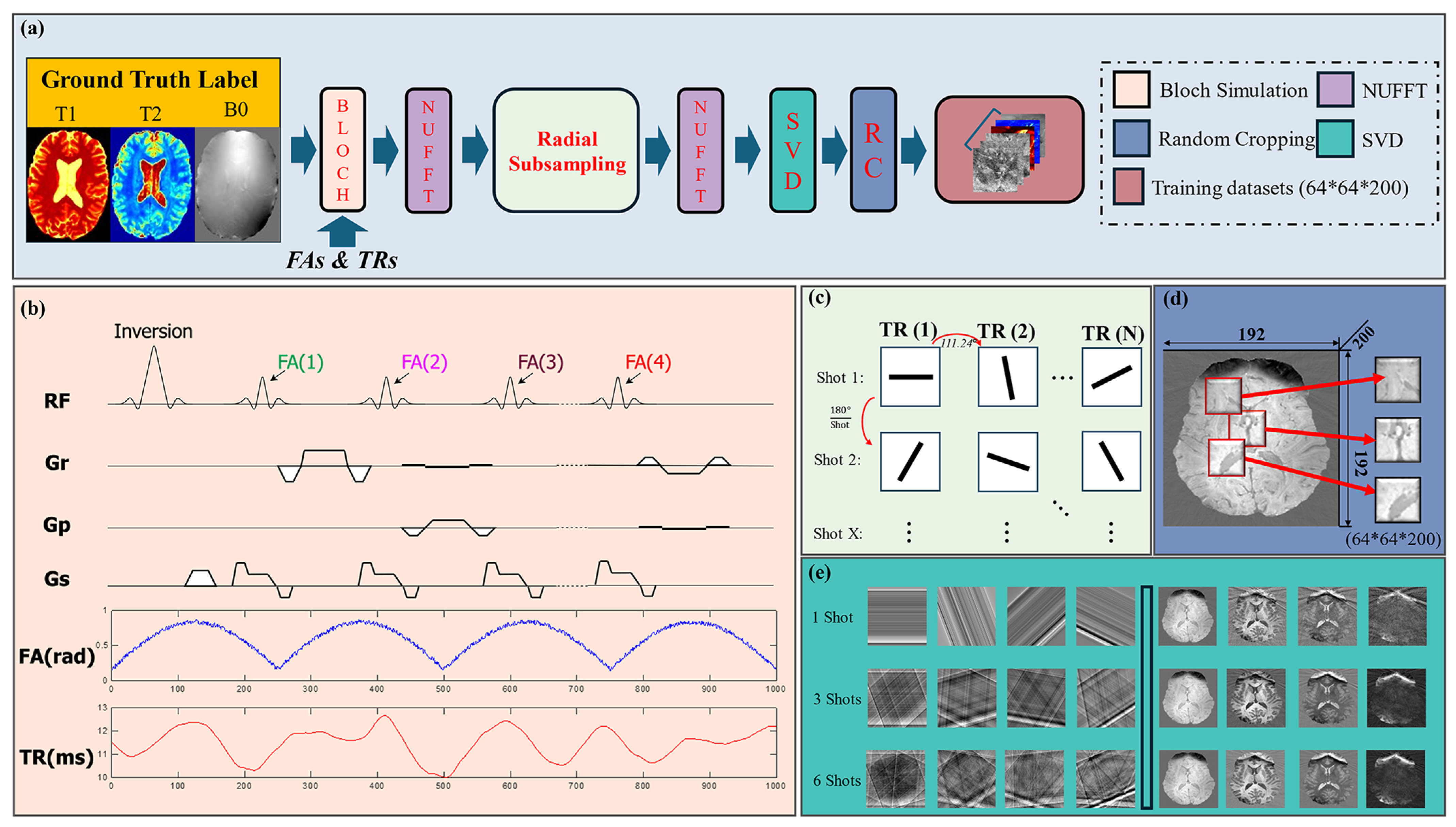
2.1. MRF Pulse Sequences and Simulations

In this study, we implemented the inversion-recovery balanced steady-state free precession (IR-bSSFP) sequence as proposed in the original MRF paper [3], and which is particularly sensitive to T1, T2, and off-resonance frequencies. Figure 1a shows the whole self-supervised dataset generation process.
The sequence consists of 1000 IR-bSSFP repetitions with varying flip angles (FAs) and repetition times (TRs). Voxel-wise signal evolution for any given tissue parameter set (i.e., T1, T2, and off-resonance frequency B0) can be synthesized using the Bloch equation:
S I m a g e = Bloch T 1 , T 2 , B 0 , F A s , T R s

2.2. Undersampling and Aliasing Effects

To accelerate the MRF scans, each image at a given time point in the MRF series needs to be highly undersampled. In this study, we implemented a radial undersampling scheme, as described in [27]. Each radial readout is rotated by the golden angle relative to the previous one. The k-space sampling trajectory is denoted as k t r j . A single-shot MRF acquisition is completed after 1000 TR. Severe aliasing artifacts, as a result of the aggressive undersampling, can be seen in Figure 1e. To mitigate these effects, multiple-shot acquisitions can be performed at the cost of increased scan time. In this study, we also conducted 3-shot and 6-shot acquisitions by repeating the single-shot acquisition 3 and 6 times, respectively, with a signal recovery period of 10 s between shots and rotating the radial readout arms by 60 (3 shots) degrees and 30 (6 shots) degrees between consecutive shots. The sampling trajectories of the multi-shot scans were formed by merging the individual k t r j from each shot. Simulated k-space acquisitions can be modelled using the NUFFT package as follows:
S K s p a c e _ r a d i a l = NUFFT ( S I m a g e ,   k t r j )
where S K s p a c e _ r a d i a l represents the simulated radial MRF k-space acquisition, and the N U F F T operation computes the radial undersampled k-space for different radial arm trajectories. The aliased image from the direct inverse NUFFT is generated as follows:
S I m a g e _ a l i a s e d = N U F F T 1 ( S K s p a c e _ r a d i a l ,   k t r j )

2.3. Synthetic Training Dataset

The training datasets were simulated through a high-resolution ME-MP2RAGE [28] dataset to construct T1, T2*, and B0 images from ten healthy volunteers. Institutional ethics board approval was obtained, and all subjects gave informed written consent. The T2 labels for the MRF simulation were synthesized from the T2* images by scaling with a factor of 1.5. As shown in Figure 1, we then employed steps (1) to (3), as described above, to synthesize the training datasets. A total number of 1500 paired training samples of a size of 192 × 192 pixels were generated, with the aliased MRF image series as input, and with sources T1 and T2 as labels.

2.4. Time Series Dimension Reduction

To optimize the reconstruction quality, singular value decomposition (SVD) was applied to compress the temporal dimension from 1000 to 200 [7]. By reducing the size of the temporal dimension, computational resources are conserved, as smaller datasets demand less memory and processing power during training and inference. Additionally, the compression allows for the generation of an expanded training dataset, as the reduced size enables more samples to fit within the same computational budget. Importantly, the accuracy of the MRF reconstruction using SVD is well maintained [7]. The singular metric was derived from the dictionary. This compression yields a refined training dataset with dimensions of 192 × 192 × 200. Three highly subsampled acquisitions (1, 3, and 6 radial sampling arms, respectively) were simulated in this work to mimic the real-world radial MRF acquisitions. For in vivo scans, the 1000-timepoint MRF signal was also reduced to 200 timepoints using the same SVD method as in the MRF simulation dataset.

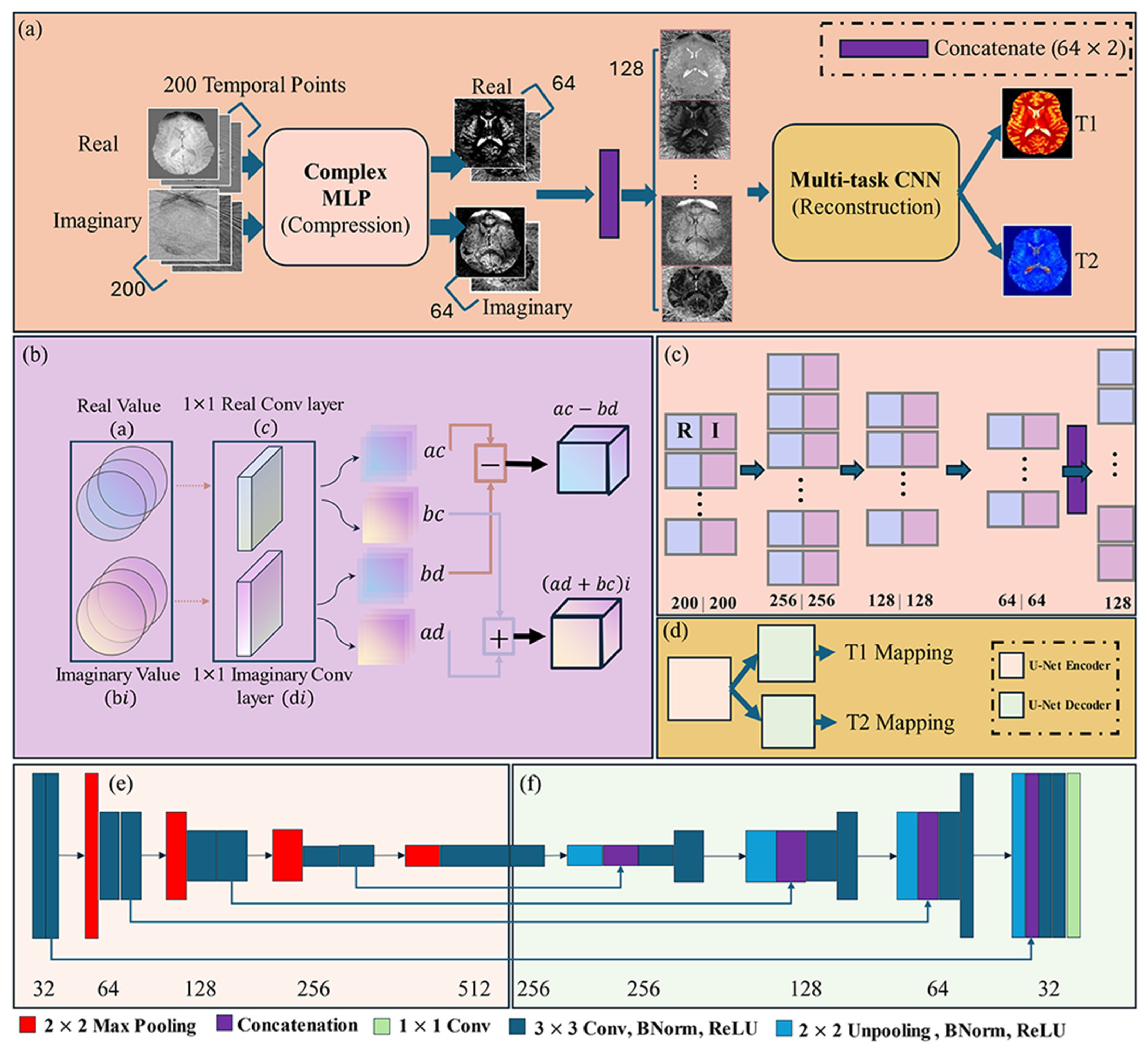
2.5. MRF-Mixer Neural Network

Figure 2 illustrates our proposed MRF-Mixer network architecture, which integrates two key components. These two components efficiently handle the complex spatio-temporal nature of MRF data. The complex MLP performs compression, and extracts relevant temporal features, and the multi-task U-Net refines spatial consistency in the reconstructed parameter maps, addressing the limitations of previous methods.

2.5.1. Complex-Valued Multi-Layer Perceptron (cMLP)

The complex-valued MLP (cMLP), implemented by the convolutional operation with kernel size of 1 × 1, consists of two hidden layers that reduce the input from 200 to 64 channels. During this dimension reduction process, and as shown in Algorithm 1, the operations in these two hidden layers are performed on both the real and imaginary components, following the procedures detailed in Algorithm 2.
Algorithm 1 MRF-Mixer Complex-MLP Block
Input:  X r ,   X i R b × 200 × H × W
Hyperparameters:
                                EncodingDepth = 2, n 0 = 256
1Step 1: Initial Complex Convolution
2                                    X r , X i C C o n v L a y e r   X r , X i , 200 , n 0
3for  l = 1  to EncodingDepth do
4           n l n 0 2 l 1
5          Step 2: Complex Conv Layer with n l output channels
6                                                Y r , Y i C C o n v L a y e r   X r , X i , n l , n l / 2
7          Step 3: Residual Connection
8                                       X r , X i C C o n v L a y e r   Y r + X r , Y r + X i , n l / 2 , n l / 2
9end for
Output:  X r , X i R b × 64 × H × W
Algorithm 2 Complex Convolution (CCovnLayer) with 1 × 1 Kernel Size
Input: Complex feature map X = a + i b   ( X r , X i )
Trainable Parameters:
                                    Complex convolution weights
                                     W = c + i d
1Step 1: Complex Convolution
2Compute Y r = a c b d
3                                                      ➢    denotes standard real-valued convolution
4Compute Y i = a d b c
5                                                      ➢    denotes standard real-valued convolution
6Step 2: Batch Normalization
7 Y r B a t c h N o r m   Y r
8 Y i B a t c h N o r m   Y i
Output:  Y = Y r + i Y i
The basic network layer can be written as follows:
y 0 = R e L U B N W 0 x 0 + b 0
Take the first layer as example, W 0 C 256 × 200 × 1 × 1 and b 0 C 256 × 1 represent the complex convolutional kernel and bias, respectively, and C is the complex number set; B N and R e L U represent the conventional batch-normalization operation and the rectified linear unit activation function, which are applied separately to the real and imaginary components of the complex feature maps; is the complex convolution operation; and y 0 represents the output features of this layer.
Figure 2b demonstrates the proposed complex MLP-like convolution. The introduced complex convolutional layer with 1 × 1 convolution kernel, which is developed based on the multiplication rules of complex numbers [29,30] and DCRNet [31]. The complex convolution between a complex input X = a + b i and a complex 1 × 1 convolution kernel W = c + d i is represented as follows:
Y = X W
The complex multiplication in the MLP structure also allows interconnected processing of real and imaginary components, retaining all of the information present in the training data. The necessity to employ a complex convolutional operation stems from several considerations. This can be supported by the existing literature [12], which showcased that both the real and imaginary components of data harbor critical information, making it beneficial to utilize them conjointly for tissue property reconstruction. Prior studies [12] have also demonstrated that leveraging both real and imaginary parts of complex MRF signals can significantly reduce quantification errors compared with methods that use only the magnitude of signals.

2.5.2. Multi-Task CNN (U-Net)

The CNN-based U-Net processes spatial information and reconstructs tissue parameter maps. It consists of a shared encoder that receives the output from the cMLP, branching into two distinct decoders—each focused on reconstructing one of the tissue properties (T1 and T2). As demonstrated in Algorithm 3, the detailed structure of the Multi-Task U-Net addresses the challenge of inter-parameter effects, enabling more targeted and accurate parameter estimation.
Algorithm 3 Multi-Task U-Net
Input:  X R b × 128 × H × W                                                       ➢   Output from cMLP
Hyperparameters:
             EncodingDepth = 4, I n   c h a n n e l s = 128 ,   O u t   c h a n n e l s = 1
1unet  Unet (EncodingDepth, In channels, Out channels)
2Step 1: Encoding in U-Net:
3                                                 X , s t a t e s U n e t _ E n c o d e r   ( X )
4Step 2: Multi Decoders for T1, T2, B0 & PVs:
                                                X T 1 U n e t _ D e c o d e r T 1   ( X , s t a t e s )
                                                X T 2 U n e t _ D e c o d e r T 2   ( X , s t a t e s )
                                      X P V s S o f t m a x ( U n e t _ D e c o d e r P V s   ( X , s t a t e s ) )
Output:  X T 1 , X T 2 , ( X P V s )                                 ➢   Only T1, T2 maps in this work
Furthermore, the Multi-Task U-Net architecture demonstrates flexibility for expansion to reconstruct additional tissue maps simultaneously. The architecture shows promising potential for partial volume estimation applications, as indicated by the framework in Algorithm 3. The incorporation of a dedicated layer with appropriate training data could enable partial volume quantification, though this remains as future work to be explored.

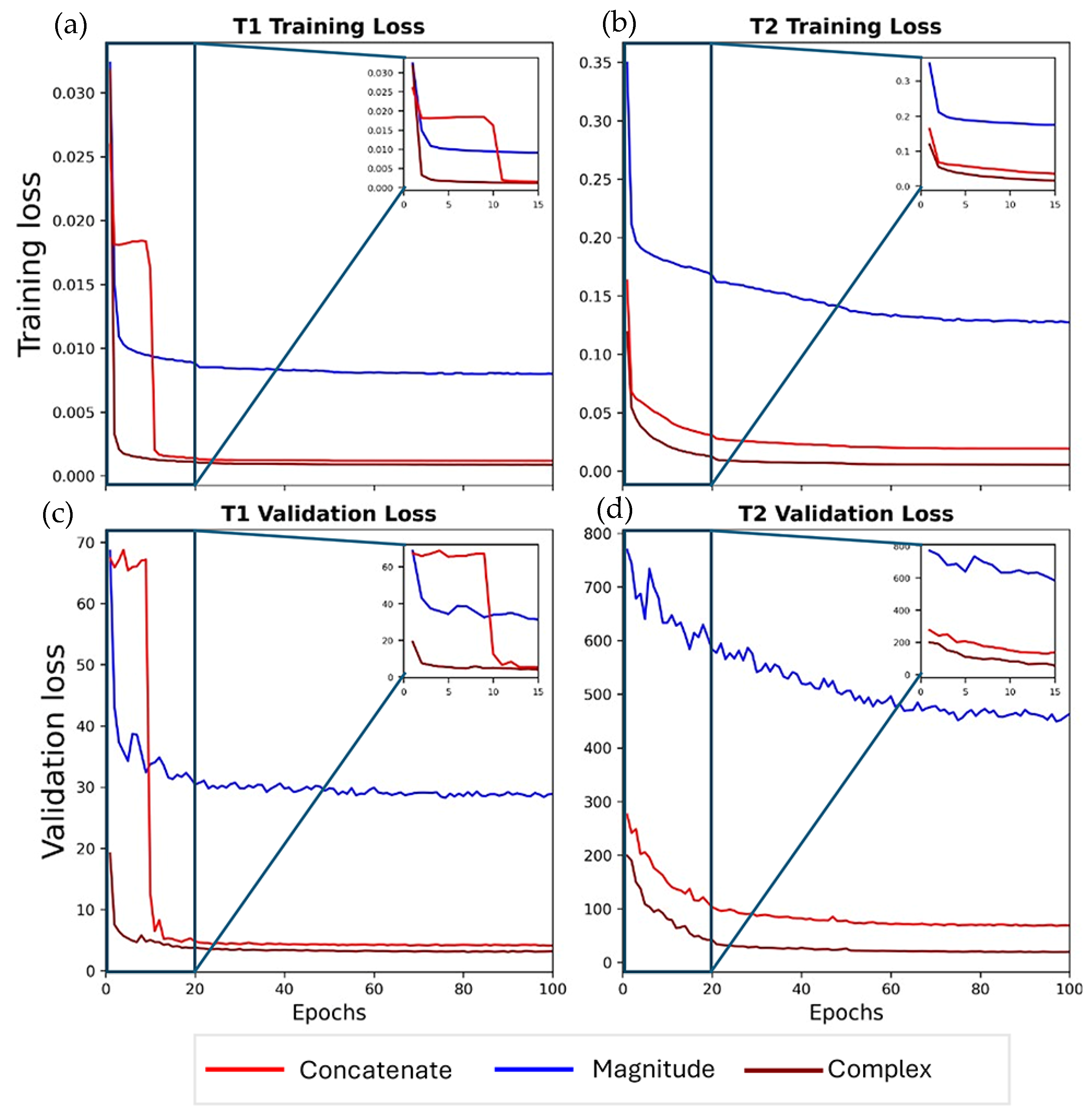
2.6. Network Training

A total of 1500 images (each 192 × 192 pixels) was simulated from ten ME-MP2RAGE brain scans and then randomly cropped into 30,000 image patches of size 64 × 64 for network training. All network parameters were initialized with normally distributed random numbers (mean = 0, standard deviation = 0.01). For training MRF-Mixer, we used the ADAM optimizer with a mean squared error (MSE) loss function and trained for 100 epochs on an Nvidia Tesla H100 GPU. The training process took approximately 13 h. We set the batch size to 8 and the initial learning rate to 0.001, which decayed by half every 25 epochs.

2.7. Evaluation Experiments

To evaluate the performance of MRF-Mixer, we conducted three ablation studies to demonstrate the necessity of our proposed approach. In the first study, we compared the effect of SVD for model training. In the second ablation study, we compared training and validation loss when using a complex-valued multiplication process versus using the magnitude of the signal and concatenating real and imaginary values for training. All methods employed a similar network structure, maintaining consistent input and output channels. The third ablation study examined whether using multiple U-Net decoders improves performance compared with using a single U-Net decoder or no U-Net. The model without U-Net refers to the cMLP model from the first ablation study, where the channels are reduced to two (i.e., T1 and T2) via several hidden complex convolutional layers.

2.7.1. Simulation Dataset

A synthetic evaluation test set was generated using the same process as for training, but from a different volunteer, one who was not included in the training data. This dataset was used to assess model performance through quantitative and qualitative analysis of simulation results.

2.7.2. In Vivo Experiments

In vivo data were acquired from a healthy volunteer using a 3T scanner (Siemens Prisma, Erlangen, Germany) with a 32-channel head coil. The volunteer was scanned across 32 slices using a 1000-timepoint IR-bSSFP pulse sequence with a 1 mm in-plane resolution and a 3 mm slice thickness and varying radial sampling arms. Written informed consent was obtained from the volunteer prior to participating in this study. The in vivo dataset was used to compare the reconstruction quality of different models in real-world conditions.

2.7.3. Comparison with Other Methods

To compare with conventional dictionary-matching (DM) methods, we created an MRF dictionary using the Bloch equation simulator, containing 643,200 MRF dictionary pairs (T1 range: 100–4000 ms, with 100 ms step, T2 range: 10–800 ms with 10 ms step, and B0 range: −200–200 Hz, with 2 Hz step).
For the deep learning method, we conducted comparative analyses against three established deep learning methods: DRONE [11], SCQ [12], CONV-ICA [19] and cMLP. In implementing DRONE, we adhered to its standard framework, utilizing magnitude data as the training input. For the SCQ method, we adopted the two-step model architecture as described in their work but trained it on our synthetic dataset due to the unavailability of their pre-trained dataset. For CONV-ICA, we diverged from the original methodology, which employed magnitude values from MRF signals, and instead trained the network using our synthetic dataset. Notably, for DRONE [11], the original study used the FISP sequence, whereas we employed the IR-bSSFP sequence, resulting in differences in the dictionaries. Training with our dictionary produced suboptimal results compared with using our synthetic dataset. Similarly, for SCQ [12], we were unable to replicate their pre-training step entirely, so we limited our adaptation to their network structure. Our implementation instead employed complex values, as this modification demonstrated superior performance in our experiments.

2.8. Evaluation Metrics

To evaluate the quality of the reconstructed parametric maps, we use four widely adopted metrics: root mean square error (RMSE), mean absolute error (MAE), peak signal-to-noise ratio (PSNR), and structural similarity index (SSIM).
To evaluate the in vivo experimental results, we compare the tissue parameter maps of different methods from 1, 3, and 6 shots to validate the consistency among different shots. We compare these methods both qualitatively and quantitively on their artifact reduction, noise improvement, and report their quantitative T1, and T2 values and standard deviations of multiple brain regions.

3. Results

3.1. Ablation Study

We evaluated the impact of using complex-valued operations versus magnitude-based methods and concatenation-based methods for MRF reconstruction, as shown in Figure 3.
The results demonstrate that the complex method outperforms the magnitude-based method in both training and validation across T1 and T2 estimations. The complex method achieves faster convergence and lower final losses, particularly for T2, where the magnitude method shows significant fluctuations and slower convergence. The concatenation method (i.e., concatenate the real and imaginary channels as an input for real-valued operation) performs similarly to the complex method, yielding slightly higher training and validation losses. These findings highlight the importance of using complex-valued representations for improved accuracy and stability in MRF parameter estimation.
Table 1 compares the performance of cMLP (without U-Net), single-branch (Single Encoder-Single Decoder U-Net), and MRF-Mixer (Multi-Decoder U-Net) models for estimating T1 and T2. While both U-Net variants significantly outperform cMLP across all metrics, the multi-task MRF-Mixer demonstrates distinct advantages in T1 estimation with statistically significant improvements over the single-branch U-Net. For T2 estimation, both U-Net architectures achieve comparable performance, with no statistically significant differences observed.

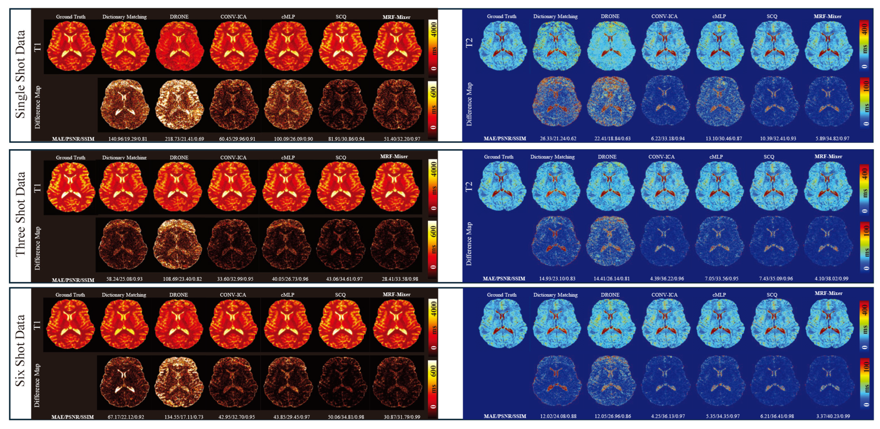
3.2. Simulation Results

Figure 4 provides a comparative evaluation of DM, DRONE, CONV-ICA, cMLP, SCQ and MRF-Mixer using single-shot, three-shot, and six-shot MRF datasets.
While our proposed MRF-Mixer demonstrates strong overall performance in both T1 and T2 mapping, achieving the lowest MAE and highest PSNR and SSIM in most cases, it is important to note that certain results from the SCQ method slightly outperform the MRF-Mixer. Nonetheless, the MRF-Mixer maintains a PSNR of more than 31 and an SSIM above 0.97 in T1 mapping, and a PSNR exceeding 34 with an SSIM of 0.97 in T2 mapping, illustrating its robustness and reliability compared with other methods overall.
Table 2 and Table 3 provides a quantitative comparison of the performance of the different methods under varying shot numbers for both T1 and T2 maps.
The metrics considered include MAE, PSNR, SSIM, and RMSE. MRF-Mixer achieves the best results, followed by CONV-ICA, for most of these metrics, as highlighted in bold. For the one-shot scenario, MRF-Mixer achieves the lowest MAE of 48.63 ± 5.03 for T1 and 9.25 ± 3.34 for T2, outperforming other models. The PSNR and SSIM values for MRF-Mixer are also the highest, reaching 30.81 ± 1.35 and 0.96 ± 0.00, respectively, in T1 mapping, indicating more accurate signal reconstruction and structural similarity to ground truth data. For the three-shot and six-shot scenarios, MRF-Mixer continues to outperform other methods, with the lowest MAE and RMSE values, indicating improved accuracy in both T1 and T2 mapping as shot numbers increase.

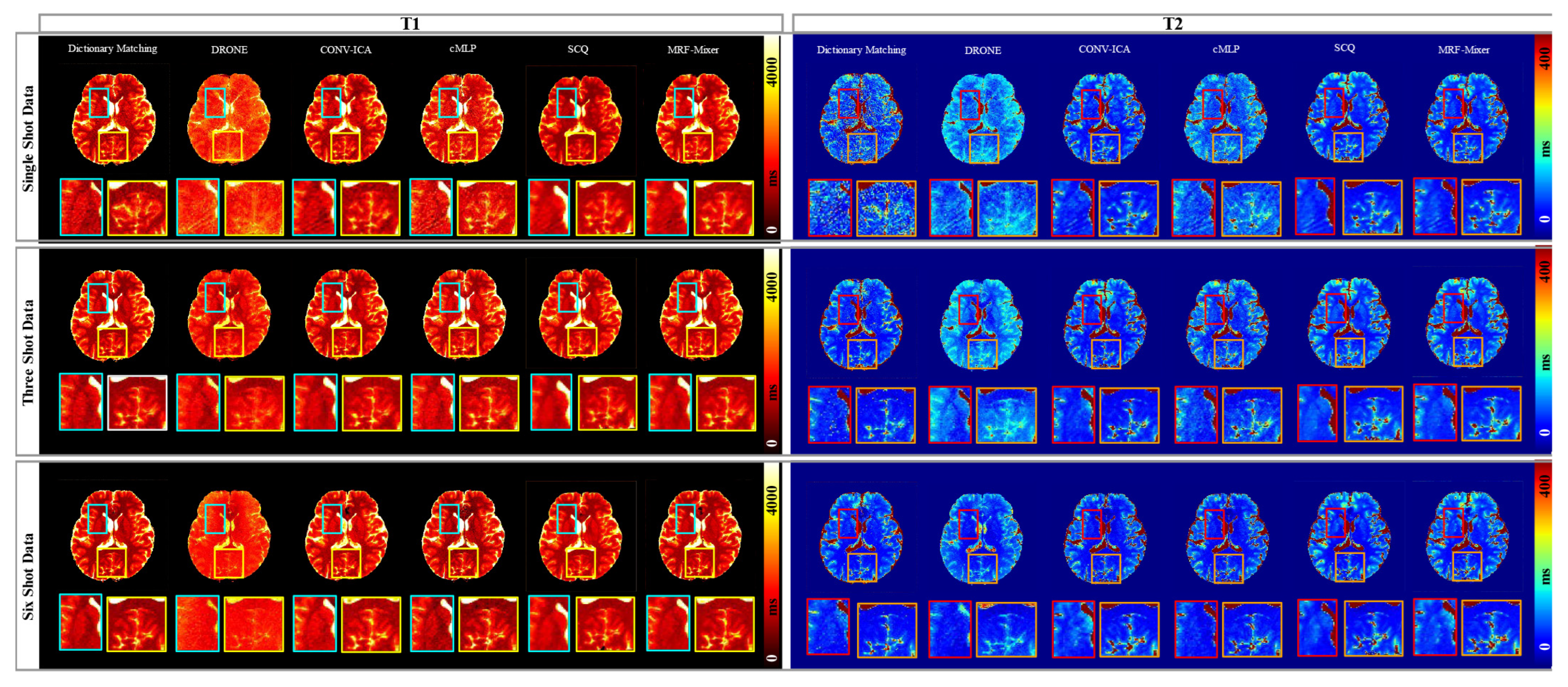
3.3. In Vivo Experimental Results

Figure 5 illustrates the comparison of DM, DRONE, CONV-ICA, cMLP, SCQ and MRF-Mixer of in vivo quantitative T1 and T2 brain mappings of a healthy volunteer at 3T with 1 mm isotropic resolution in 1, 3, and 6 radial arms. The proposed MRF-Mixer method reveals significant advantages, particularly in single-shot acquisition scenarios. The MRF-Mixer secures two key benefits: it facilitates the reconstruction of high-quality T1 and T2 maps from single-shot data, and it sustains consistent performance across single-, three- and six-shot acquisitions. Additionally, the quality of single-shot reconstructions by MRF-Mixer is comparable to that of the six-shot reconstructions by DM (as a gold-standard reference result).
Table 4 and Table 5 present T1 and T2 values for all evaluated methods across three combined tissue regions as shown in Figure A1. In the WM region, MRF-Mixer showed improved precision with single-shot acquisition, yielding T1 values of 969.52 ± 48.33 ms compared with DM’s 909.28 ± 134.35 ms, suggesting reduced variance. The mean ± SD values obtained by MRF-Mixer for CSF, WM, and GM regions appear consistent with previously reported literature values [14,32,33] and show similarity with measurements from CONV-ICA SCQ, and cMLP methods, supporting the method’s accuracy. One potential limitation of the conventional DM method can be observed in the CSF value of 4000 ± 0 ms in six-shot acquisition, indicating that the matching result may be constrained by the dictionary range. This constraint could potentially affect accuracy in more complex scenarios.
The improved precision of MRF-Mixer is reflected in the reduced standard deviations across various acquisition protocols. This trend suggests a possible relationship between increased acquisition information and enhanced reconstruction precision. The results indicate that MRF-Mixer tends to provide more precise measurements across the three tissue types and acquisition methods, as suggested by the generally smaller standard deviations in both T1 and T2 measurements compared with the DM method. These observations point to the potential reliability of the MRF-Mixer approach in quantitative tissue characterization.

4. Discussion

This study presents a novel deep learning method, MRF-Mixer, aimed at overcoming limitations in conventional dictionary matching approaches for MRF reconstruction. Our work addresses several key challenges in existing techniques, including the computational burden of dictionary matching (DM) and potential inaccuracies in deep learning models that rely on DM for training label construction.
The implementation of a complex-valued neural network preserves both real and imaginary information and, when combined with our spatio-temporal network structure, maximizes information extraction from MRF datasets, contributing to the superior performance observed in our results. This integrated design capitalizes on the complementary strengths of each component: the former encoder excels at modeling intricate spatial relationships, while the U-Net architecture provides robust multi-scale feature extraction. The synergy between these components significantly enhances both spatial representation capabilities and overall reconstruction accuracy.
Our proposed simulation-based data generation pipeline uses real subject data rather than random values, ensuring consistency in data preparation and enabling unbiased comparisons across different sequences, ultimately enhancing reproducibility. This approach not only demonstrates the robustness of our study but also its potential for extension to more complex tissue characterization tasks using comprehensive biophysical models in the future.
Our findings demonstrate that MRF-Mixer consistently outperforms conventional DM and existing deep learning methods like DRONE [11] SCQ [12] and CONV-ICA [19] in both simulated and in vivo experiments. Furthermore, the ability for MRF-Mixer to achieve high-quality reconstructions from single-shot acquisitions represents a significant advancement, potentially reducing scan times without compromising image quality. This is particularly evident in the comparable quality between single-shot reconstructions using our methods and six-shot reconstructions using DM.
Moreover, the analysis of quantitative T1 and T2 relaxation times in various brain regions reveals that our proposed methods produce values consistent with the literature [14,32,33], while potentially offering a more nuanced representation of tissue characteristics. The consistent performance of MRF-Mixer across different ROIs suggests enhanced precision in quantitative tissue characterization. The reduced variability in T1 and T2 estimations highlights the method’s potential for more reliable and accurate tissue property assessments in clinical and research settings.
The results of our methodology demonstrate significant promise, yet we acknowledge the need for further validation using larger and more diverse datasets to establish true generalizability. Furthermore, evaluation across various pathological conditions and anatomical structures remains an essential next step in validating our approach. Future research directions should focus on further optimization of these models, exploration of their applicability to a wider range of tissue types, and investigation of their potential for partial volume estimation in MRF signal evolution. The expansion of pulse sequence investigations beyond IR-bSSFP would provide valuable insights into sequence-dependent performance variations. The integration of these advanced reconstruction techniques with emerging MRF acquisition strategies, coupled with architectural optimizations to reduce parameter counts, could lead to even more significant improvements in quantitative MRI while enhancing clinical applicability and reducing computational demands.

5. Conclusions

MRF-Mixer represents a significant advancement in quantitative MRI by enhancing both reconstruction accuracy and computational efficiency compared with conventional dictionary matching and existing deep learning approaches. The ability to achieve high-quality single-shot reconstructions further underscores its potential to reduce scan times without compromising image fidelity. Future work will focus on expanding validation across diverse anatomical structures and pathological conditions, refining network architecture for greater efficiency, and extending investigations to additional pulse sequences.

Author Contributions

Methodology, T.D., Y.G. and H.S.; Software, Y.G.; Validation, Z.X.; Investigation, T.D., Y.G. and Z.X.; Resources, H.S.; Data curation, M.A.C.; Writing—original draft, T.D.; Writing—review & editing, M.A.C. and H.S.; Visualization, T.D.; Supervision, F.L. and H.S.; Funding acquisition, F.L. and H.S. All authors have read and agreed to the published version of the manuscript.

Funding

This work was supported in part by the Australian Research Council under Grant DE210101297 and Grant DP230101628, and by the National Health and Medical Research Council of Australia under Grant 2030157, and by National Natural Science Foundation of China under Grant 62301616, and by Natural Science Foundation of Hunan under Grant 2024JJ6530.

Institutional Review Board Statement

The study was conducted in accordance with the Declaration of Helsinki, and approved by the Institutional Review Board of the University of Queensland (Centre for Advanced Imaging development ethics, 26 March 2021).

Informed Consent Statement

Informed consent was obtained from all subjects involved in the study.

Data Availability Statement

The data presented in this study are available on request from the corresponding author.

Conflicts of Interest

The authors declare no conflict of interest.

Appendix A

Selected ROI for T1 and T2 values in Table 4 and Table 5
Figure A1. Selected ROI for Table 4 and Table 5.
Information 16 00218 g0a1

References

  1. Cashmore, M.T.; McCann, A.J.; Wastling, S.J.; McGrath, C.; Thornton, J.; Hall, M.G. Clinical quantitative MRI and the need for metrology. Br. J. Radiol. 2021, 94, 20201215. [Google Scholar] [CrossRef] [PubMed]
  2. Gómez, P.A.; Cencini, M.; Golbabaee, M.; Schulte, R.F.; Pirkl, C.; Horvath, I.; Fallo, G.; Peretti, L.; Tosetti, M.; Menze, B.H.; et al. Rapid three-dimensional multiparametric MRI with quantitative transient-state imaging. Sci. Rep. 2020, 10, 13769. [Google Scholar] [CrossRef] [PubMed]
  3. Ma, D.; Gulani, V.; Seiberlich, N.; Liu, K.; Sunshine, J.L.; Duerk, J.L.; Griswold, M.A. Magnetic resonance fingerprinting. Nature 2013, 495, 187–192. [Google Scholar] [CrossRef] [PubMed]
  4. Deshmane, A.; McGivney, D.F.; Ma, D.; Jiang, Y.; Badve, C.; Gulani, V.; Seiberlich, N.; Griswold, M.A. Partial volume mapping using magnetic resonance fingerprinting. NMR Biomed. 2019, 32, e4082. [Google Scholar] [CrossRef]
  5. McGivney, D.F.; Boyacıoğlu, R.; Jiang, Y.; Poorman, M.E.; Seiberlich, N.; Gulani, V.; Keenan, K.E.; Griswold, M.A.; Ma, D. Magnetic resonance fingerprinting review part 2: Technique and directions. J. Magn. Reson. Imaging 2020, 51, 993–1007. [Google Scholar] [CrossRef]
  6. Cauley, S.F.; Setsompop, K.; Ma, D.; Jiang, Y.; Ye, H.; Adalsteinsson, E.; Griswold, M.A.; Wald, L.L. Fast group matching for MR fingerprinting reconstruction. Magn. Reson. Med. 2015, 74, 523–528. [Google Scholar] [CrossRef]
  7. McGivney, D.F.; Pierre, E.; Ma, D.; Jiang, Y.; Saybasili, H.; Gulani, V.; Griswold, M.A. SVD Compression for Magnetic Resonance Fingerprinting in the Time Domain. IEEE Trans. Med Imaging 2014, 33, 2311–2322. [Google Scholar] [CrossRef]
  8. Zhao, B.; Setsompop, K.; Adalsteinsson, E.; Gagoski, B.; Ye, H.; Ma, D.; Jiang, Y.; Ellen Grant, P.; Griswold, M.A.; Wald, L.L. Improved magnetic resonance fingerprinting reconstruction with low-rank and subspace modeling. Magn. Reason. Med. 2018, 79, 933–942. [Google Scholar] [CrossRef]
  9. Assländer, J.; Cloos, M.A.; Knoll, F.; Sodickson, D.K.; Hennig, J.; Lattanzi, R. Low rank alternating direction method of multipliers reconstruction for MR fingerprinting. Magn. Reson. Med. 2018, 79, 83–96. [Google Scholar] [CrossRef]
  10. Yang, M.; Ma, D.; Jiang, Y.; Hamilton, J.; Seiberlich, N.; Griswold, M.A.; McGivney, D. Low rank approximation methods for MR fingerprinting with large scale dictionaries. Magn. Reson. Med. 2018, 79, 2392–2400. [Google Scholar] [CrossRef]
  11. Cohen, O.; Zhu, B.; Rosen, M.S. MR fingerprinting deep reconstruction network (DRONE). Magn. Reason. Med. 2018, 80, 885–894. [Google Scholar] [CrossRef] [PubMed]
  12. Fang, Z.; Chen, Y.; Liu, M.; Xiang, L.; Zhang, Q.; Wang, Q.; Lin, W.; Shen, D. Deep Learning for Fast and Spatially Constrained Tissue Quantification From Highly Accelerated Data in Magnetic Resonance Fingerprinting. IEEE Trans. Med. Imaging 2019, 38, 2364–2374. [Google Scholar] [CrossRef] [PubMed]
  13. Barbieri, M.; Brizi, L.; Giampieri, E.; Solera, F.; Manners, D.N.; Castellani, G.; Testa, C.; Remondini, D. A deep learning approach for magnetic resonance fingerprinting: Scaling capabilities and good training practices investigated by simulations. Phys. Med. 2021, 89, 80–92. [Google Scholar] [CrossRef] [PubMed]
  14. Chen, Y.; Fang, Z.; Hung, S.-C.; Chang, W.-T.; Shen, D.; Lin, W. High-resolution 3D MR Fingerprinting using parallel imaging and deep learning. NeuroImage 2020, 206, 116329. [Google Scholar] [CrossRef]
  15. Golbabaee, M.; Chen, D.; Gomez, P.A.; Menzel, M.I.; Davies, M.E. Geometry of Deep Learning for Magnetic Resonance Fingerprinting. In Proceedings of the ICASSP 2019—2019 IEEE International Conference on Acoustics, Speech and Signal Processing (ICASSP), Brighton, UK, 12–17 May 2019; pp. 7825–7829. [Google Scholar]
  16. Lundervold, S.; Lundervold, A. An overview of deep learning in medical imaging focusing on MRI. Z. Med. Phys. 2019, 29, 102–127. [Google Scholar] [CrossRef]
  17. Hoppe, E.; Körzdörfer, G.; Würfl, T.; Wetzl, J.; Lugauer, F.; Pfeuffer, J.; Maier, A. Deep learning for magnetic resonance fingerprinting: A new approach for predicting quantitative parameter values from time series. In German Medical Data Sciences: Visions and Bridges; IOS Press: Oldenburg, Germany, 2017; Volume 243, pp. 202–206. [Google Scholar] [CrossRef]
  18. Oksuz, I.; Cruz, G.; Clough, J.; Bustin, A.; Fuin, N.; Botnar, R.M.; King, A.P.; Schnabel, J.A. Magnetic Resonance Fingerprinting Using Recurrent Neural Networks. In Proceedings of the IEEE 16th International Symposium on Biomedical Imaging (ISBI 2019), Venice, Italy, 8–11 April 2019; pp. 1537–1540. [Google Scholar]
  19. Soyak, R.; Navruz, E.; Ersoy, E.O.; Cruz, G.; Prieto, C.; King, A.P.; Unay, D.; Oksuz, I. Channel Attention Networks for Robust MR Fingerprint Matching. IEEE Trans. Biomed. Eng. 2022, 69, 1398–1405. [Google Scholar] [CrossRef]
  20. Balsiger, F.; Konar, A.S.; Chikop, S.; Chandran, V.; Scheidegger, O.; Geethanath, S.; Reyes, M. Magnetic resonance fingerprinting reconstruction via spatiotemporal convolutional neural networks. In Machine Learning for Medical Image Reconstruction; Springer: Cham, Switzerland, 2018; pp. 39–46. [Google Scholar]
  21. Cao, P.; Cui, D.; Vardhanabhuti, V.; Hui, E.S. Development of fast deep learning quantification for magnetic resonance fingerprinting in vivo. Magn. Reson. Imaging 2020, 70, 81–90. [Google Scholar] [CrossRef]
  22. Song, P.; Eldar, Y.C.; Mazor, G.; Rodrigues, M.R.D. Magnetic Resonance Fingerprinting Using a Residual Convolutional Neural Network. In Proceedings of the ICASSP 2019—2019 IEEE International Conference on Acoustics, Speech and Signal Processing (ICASSP), Brighton, UK, 12–17 May 2019; pp. 1040–1044. [Google Scholar]
  23. Li, P.; Hu, Y. Deep magnetic resonance fingerprinting based on Local and Global Vision Transformer. Med. Image Anal. 2024, 95, 103198. [Google Scholar] [CrossRef]
  24. Li, P.; Hu, Y. Deep graph embedding based on Laplacian eigenmaps for MR fingerprinting reconstruction. Med. Image Anal. 2025, 101, 103481. [Google Scholar] [CrossRef]
  25. Gao, Y.; Ding, T.; Cloos, M.; Sun, H. MRF-mixer: A self-supervised deep learning MRF framework. In Proceedings of the 2023 ISMRM & ISMRT Annual Meeting, Toronto, ON, Canada, 3–8 June 2023. [Google Scholar]
  26. Ding, T.; Gao, Y.; Xiong, Z.; Cloos, M.; Sun, H. Multi Complex-valued Spatio-temporal Fusion Networks for Robust MRF Reconstruction. In Proceedings of the 2024 ISMRM & ISMRT Annual Meeting, Singapore, 4–9 May 2024. [Google Scholar]
  27. Cloos, M.A.; Assländer, J.; Abbas, B.; Fishbaugh, J.; Babb, J.S.; Gerig, G.; Lattanzi, R. Rapid Radial T1 and T2 Mapping of the Hip Articular Cartilage with Magnetic Resonance Fingerprinting. J. Magn. Reson. Imaging 2019, 50, 810–815. [Google Scholar] [CrossRef]
  28. Sun, H.; Cleary, J.O.; Glarin, R.; Kolbe, S.C.; Ordidge, R.J.; Moffat, B.A.; Pike, G.B. Extracting more for less: Multi-echo MP2RAGE for simultaneous T1-weighted imaging, T1 mapping, mapping, SWI, and QSM from a single acquisition. Magn. Reson. Med. 2020, 83, 1178–1191. [Google Scholar] [CrossRef] [PubMed]
  29. El-Rewaidy, H.; Neisius, U.; Mancio, J.; Kucukseymen, S.; Rodriguez, J.; Paskavitz, A.; Menze, B.; Nezafat, R. Deep complex convolutional network for fast reconstruction of 3D late gadolinium enhancement cardiac MRI. NMR Biomed. 2020, 33, e4312. [Google Scholar] [CrossRef] [PubMed]
  30. Wang, S.; Cheng, H.; Ying, L.; Xiao, T.; Ke, Z.; Zheng, H.; Liang, D. DeepcomplexMRI: Exploiting deep residual network for fast parallel MR imaging with complex convolution. Magn. Reson. Imaging 2020, 68, 136–147. [Google Scholar] [CrossRef] [PubMed]
  31. Gao, Y.; Cloos, M.; Liu, F.; Crozier, S.; Pike, G.B.; Sun, H. Accelerating quantitative susceptibility and R2* mapping using incoherent undersampling and deep neural network reconstruction. NeuroImage 2021, 240, 118404. [Google Scholar] [CrossRef]
  32. Ma, S.; Wang, N.; Fan, Z.; Kaisey, M.; Sicotte, N.L.; Christodoulou, A.G.; Li, D. Three-dimensional whole-brain simultaneous T1, T2, and T1ρ quantification using MR Multitasking: Method and initial clinical experience in tissue characterization of multiple sclerosis. Magn. Reson. Med. 2021, 85, 1938–1952. [Google Scholar] [CrossRef]
  33. Deoni, S.C. High-resolution T1 mapping of the brain at 3T with driven equilibrium single pulse observation of T1 with high-speed incorporation of RF field inhomogeneities (DESPOT1-HIFI). J. Magn. Reson. Imaging 2007, 26, 1106–1111. [Google Scholar] [CrossRef]
Figure 1. (a) Self-supervised synthetic MRF data generation process. (b) Pulse sequences, FAs and TRs. (c) Radial subsampling demonstration. (d) Random cropping for simulated dataset. (e) First four timepoint images before and after SVD.
Information 16 00218 g001
Figure 2. (a) Overall MRF-Mixer structure. (b) Complex number multiplication. (c) Complex MLP (cMLP). (d) Multi-task CNN (U-Net). (e) U-Net encoder. (f) U-Net decoder.
Information 16 00218 g002
Figure 3. Training and validation loss comparison for concatenate, magnitude and complex methods: (a) T1 training loss, (b) T2 training loss, (c) T1 validation loss, and (d) T2 validation loss.
Information 16 00218 g003
Figure 4. Comparison of T1 and T2 mapping results using different methods for single-shot, three-shot, and six-shot data.
Information 16 00218 g004
Figure 5. In vivo T1 and T2 mappings for DM, DRONE, CONV-ICA, SCQ, cMLP and MRF-Mixer.
Information 16 00218 g005
Table 1. Comparison of model performance for T1 and T2 estimation. Arrows indicate whether higher ( ) or lower (↓) values are better. Best values are highlighted in bold.
ModelPropertyMAE ( )PSNR (dB) ( )SSIM ( )RMSE ( )
cMLP
(without U-Net)
T1 110.05 ± 7.62 28.75 ± 0.53 0.92 ± 0.01 168.92 ± 13.89
T2 20.37 ± 4.48 29.61 ± 1.47 0.90 ± 0.02 35.26 ± 8.18
Single-Branch
(single decoder U-Net)
T1 79.26 ± 6.66 *** 31.68 ± 0.46 *** 0.96 ± 0.00 *** 120.50 ± 9.88 ***
T2 11.27 ± 3.57 34.00 ± 2.11 0.96 ± 0.01 21.69 ± 7.44
MRF-Mixer
(multi decoder U-Net)
T1 66.49 ± 4.25 33.03 ± 0.30 0.97 ± 0.00 103.03 ± 6.09
T2 11.25 ± 3.52 33.98 ± 2.10 0.96 ± 0.01 21.74 ± 7.45
*** indicates statistically significant differences ( p < 0.001 ) between single-branch and MRF-Mixer for T1 metrics (MAE, PSNR, SSIM, RMSE). No significant differences were found for T1 metrics.
Table 2. Performance comparison of different models under varying shot numbers for T1 metrics. Arrows indicate whether higher ( ) or lower (↓) values are better. Best values are highlighted in bold.
Shot ModelT1 Metrics
MAE ( )PSNR ( )SSIM ( )RMSE ( )
1-shotMRF-Mixer48.63  ±  5.0330.81  ±  1.350.96  ±  0.00102.01  ±  9.63
cMLP94.56 ± 10.3621.70 ± 1.810.88 ± 0.02179.71 ± 18.95
CONV-ICA58.04 ± 8.12 ***27.5 ± 2.49 ***0.81 ± 0.06 ***116.97 ± 13.75 ***
DRONE221.86 ± 33.1916.57 ± 1.650.41 ± 0.06404.07 ± 50.95
DM105.96 ± 13.3723.31 ± 0.650.85 ± 0.01260.29 ± 25.64
SCQ76.34 ± 9.61 30.13 ± 0.690.92 ± 0.01120.87 ± 13.00
3-shotMRF-Mixer33.42  ±  4.8633.01  ±  1.910.98  ±  0.0078.68  ±  9.53
cMLP46.06 ± 8.6225.99 ± 2.650.95 ± 0.02103.72 ± 15.38
CONV-ICA39.92 ± 6.27 ***29.59 ± 2.45 ***0.97 ± 0.01 ***88.27 ± 10.95 ***
DRONE126.09 ± 21.2016.90 ± 2.020.53 ± 0.02275.60 ± 42.21
DM61.64 ± 9.2625.95 ± 0.920.93 ± 0.01182.62 ± 23.60
SCQ52.41 ± 9.7333.21 ± 1.030.96 ± 0.0185.22 ± 12.90
6-shotMRF-Mixer28.80  ±  4.5133.48  ±  1.830.98  ±  0.0172.90  ±  9.19
cMLP40.46 ± 7.9526.45 ± 2.800.96 ± 0.0195.32 ± 14.36
CONV-ICA35.98 ± 6.02 ***30.56 ± 2.35 ***0.83 ± 0.08 ***83.93 ± 10.87 ***
DRONE117.64 ± 28.0218.10 ± 1.700.55 ± 0.04239.19 ± 43.61
DM55.10 ± 8.2526.79 ± 0.970.94 ± 0.01162.76 ± 21.18
SCQ44.47 ± 8.3634.33 ± 1.010.97 ± 0.0174.84 ± 11.01
*** indicates statistically significant differences ( p < 0.001 ) between CONV-ICA and MRF-Mixer for T1 metrics (MAE, PSNR, SSIM, RMSE). No significant differences were found for T1 metrics.
Table 3. Performance comparison of different models under varying shot numbers for T2 metrics. Arrows indicate whether higher ( ) or lower (↓) values are better. Best values are highlighted in bold.
Shot ModelT2 Metrics
MAE ( )PSNR ( )SSIM ( )RMSE ( )
1-shotMRF-Mixer9.25 ± 3.3431.09 ± 2.610.95 ± 0.0224.00 ± 7.97
cMLP16.84 ± 3.9027.65 ± 2.100.87 ± 0.0235.68 ± 8.53
CONV-ICA9.04 ± 3.08 ***31.25 ± 2.070.90 ± 0.04 ***22.43 ± 6.94 ***
DRONE28.31 ± 6.9720.65 ± 1.350.42 ± 0.0458.83 ± 15.35
DM32.60 ± 6.0619.11 ± 0.670.65 ± 0.0390.88 ± 8.11
SCQ14.49 ± 4.7229.40 ± 2.400.93 ± 0.0230.20 ± 9.06
3-shotMRF-Mixer5.99 ± 2.2534.47 ± 2.690.98 ± 0.0116.24 ± 5.57
cMLP8.67 ± 2.6932.10 ± 1.950.96 ± 0.0120.81 ± 5.69
CONV-ICA5.97 ± 2.0334.63 ± 2.370.97 ± 0.03 ***15.28 ± 4.81 ***
DRONE15.58 ± 4.3822.32 ± 3.530.57 ± 0.0634.79 ± 9.49
DM20.40 ± 6.4221.22 ± 1.160.84 ± 0.0174.59 ± 11.67
SCQ9.76 ± 3.2032.66 ± 2.380.97 ± 0.0120.76 ± 6.33
6-shotMRF-Mixer4.97 ± 1.8735.90 ± 2.480.98 ± 0.0213.67 ± 4.62
cMLP6.90 ± 2.3533.55 ± 2.330.97 ± 0.0117.71 ± 5.34
CONV-ICA5.21 ± 1.79 ***35.33 ± 2.420.93 ± 0.04 ***13.59 ± 4.27
DRONE11.72 ± 3.1425.00 ± 2.800.64 ± 0.0526.33 ± 6.72
DM18.54 ± 6.5321.96 ± 1.400.86 ± 0.0169.71 ± 12.85
SCQ8.45 ± 2.8933.75 ± 2.560.97 ± 0.0118.42 ± 5.90
*** indicates statistically significant differences ( p < 0.001 ) ) between CONV-ICA and MRF-Mixer for T1 metrics (MAE, PSNR, SSIM, RMSE). No significant differences were found for T1 metrics.
Table 4. T1 values (ms) for each method in selected ROI.
MethodDMDRONECONV-ICAcMLPSCQMRF-Mixer
CSF1-shot3988.89 ± 21.713158.63 ± 289.794393.15 ± 277.234363.95 ± 126.973957.03 ± 141.403961.73 ± 81.46
3-shot3983.33 ± 42.832615.96 ± 320.374009.75 ± 121.584251.35 ± 132.433859.29 ± 153.103938.06 ± 82.70
6-shot4000.00 ± 0.003712.80 ± 283.224700.96 ± 113.694270.01 ± 113.104092.38 ± 48.873817.02 ± 51.93
GM1-shot1571.30 ± 196.881599.84 ± 85.381588.21 ± 138.151703.32 ± 219.841569.50 ± 111.991585.94 ± 116.21
3-shot1496.30 ± 106.711524.83 ± 90.971516.34 ± 98.451574.81 ± 104.451546.38 ± 90.601582.99 ± 103.90
6-shot1436.11 ± 126.891613.06 ± 75.641459.22 ± 103.031440.22 ± 118.101463.40 ± 30.231486.05 ± 99.85
WM1-shot909.28 ± 134.351288.99 ± 175.66912.35 ± 60.171157.50 ± 129.68946.76 ± 19.12969.52 ± 48.33
3-shot935.42 ± 71.131151.71 ± 54.82963.98 ± 66.02987.41 ± 110.88965.79 ± 45.52956.03 ± 38.14
6-shot903.47 ± 66.371361.15 ± 91.60882.75 ± 84.03875.16 ± 71.46927.48 ± 40.06916.90 ± 38.26
Table 5. T2 values (ms) for each method in selected ROI.
MethodDMDRONECONV-ICAcMLPSCQMRF-Mixer
CSF1-shot590.56 ± 98.67509.70 ± 75.66798.48 ± 40.98646.65 ± 67.85870.35 ± 37.90773.82 ± 47.57
3-shot586.94 ± 45.24450.44 ± 64.00981.58 ± 55.45774.48 ± 33.01906.94 ± 26.82883.86 ± 40.69
6-shot565.28 ± 33.09595.98 ± 54.461092.98 ± 37.41774.48 ± 33.01920.62 ± 20.78993.97 ± 28.44
GM1-shot108.61 ± 47.19111.58 ± 13.41112.61 ± 18.16124.27 ± 18.76113.15 ± 17.76120.60 ± 18.97
3-shot98.70 ± 21.00137.77 ± 13.63105.74 ± 15.46120.07 ± 21.95114.72 ± 13.99117.19 ± 17.55
6-shot83.61 ± 9.61108.01 ± 14.87100.14 ± 13.09120.07 ± 21.95101.18 ± 12.08101.96 ± 12.69
WM1-shot76.64 ± 43.5576.27 ± 16.4356.76 ± 5.7982.48 ± 15.6159.30 ± 3.5660.38 ± 5.54
3-shot56.35 ± 20.1390.64 ± 6.5155.38 ± 5.2167.15 ± 10.0661.81 ± 3.7962.35 ± 4.17
6-shot49.22 ± 7.3476.55 ± 12.9852.69 ± 5.8067.15 ± 10.0652.03 ± 3.0452.99 ± 2.88
Disclaimer/Publisher’s Note: The statements, opinions and data contained in all publications are solely those of the individual author(s) and contributor(s) and not of MDPI and/or the editor(s). MDPI and/or the editor(s) disclaim responsibility for any injury to people or property resulting from any ideas, methods, instructions or products referred to in the content.

