Time Scale in Alternative Positioning, Navigation, and Timing: New Dynamic Radio Resource Assignments and Clock Steering Strategies ^†

Abstract

Terrestrial and satellite communications, tactical data links, positioning, navigation, and timing (PNT), as well as distributed sensing will continue to require precise timing and the ability to synchronize and disseminate time effectively. However, the supply of space-qualified clocks that meet Global Navigation Satellite Systems (GNSS)-level performance standards is limited. As the awareness of potential disruptions to GNSS due to adversarial actions grows, the current reliance on GNSS-level timing appears costly and outdated. This is especially relevant given the benefits of developing robust and stable time scale references in orbit, especially as various alternatives to GNSS are being explored. The onboard realization of clock ensembles is particularly promising for applications such as those providing the on-demand dissemination of a reference time scale for navigation services via a proliferated Low-Earth Orbit (pLEO) constellation. This article investigates potential inter-satellite network architectures for coordinating time and frequency across pLEO platforms. These architectures dynamically allocate radio resources for clock data transport based on the requirements for pLEO time scale formations. Additionally, this work proposes a model-based control system for wireless networked timekeeping systems. It envisions the optimal placement of critical information concerning the implicit ensemble mean (IEM) estimation across a multi-platform clock ensemble, which can offer better stability than relying on any single ensemble member. This approach aims to reduce data traffic flexibly. By making the IEM estimation sensor more intelligent and running it on the anchor platform while also optimizing the steering of remote frequency standards on participating platforms, the networked control system can better predict the future behavior of local reference clocks paired with low-noise oscillators. This system would then send precise IEM estimation information at critical moments to ensure a common pLEO time scale is realized across all participating platforms. Clock steering is essential for establishing these time scales, and the effectiveness of the realization depends on the selected control intervals and steering techniques. To enhance performance reliability beyond what the existing Linear Quadratic Gaussian (LQG) control technique can provide, the minimal-cost-variance (MCV) control theory is proposed for clock steering operations. The steering process enabled by the MCV control technique significantly impacts the overall performance reliability of the time scale, which is generated by the onboard ensemble of compact, lightweight, and low-power clocks. This is achieved by minimizing the variance of the chi-squared random performance of LQG control while maintaining a constraint on its mean.

1. Introduction

The rapid development of pLEO constellations, composed of small satellites, has revolutionized communications and navigation services [1,2,3]. The global coverage afforded by these innovative pLEO constellations opens up unparalleled opportunities for alternative positioning, navigation, and timing (AltPNT) solutions that can reshape our technological landscape.

Navigation services utilizing one-way time-of-flight with GNSS hinge upon the meticulous monitoring of stable clocks that send out ranging signals. Each satellite houses multiple highly stable microwave clocks, all integrated into a robust timekeeping system. Managing the performance of these satellite clocks and synchronizing them with laboratory-based standards is crucial for creating an accurate time scale. This synchronization allows for reliable tracking of GNSS signals from ground reference stations worldwide. Furthermore, essential corrections are made for each satellite clock to ensure alignment with the reference time scale that is distributed to users [4,5,6].

However, it is essential to recognize that the principles underpinning GNSS are not easily applicable to LEO spacecraft, which operate with shorter lifetimes. GNSS depends on large, heavy atomic clocks, which are continuously monitored by a global network of ground stations to enable precise positioning and timing. These ground stations also upload clock corrections to maintain user accuracy. Unfortunately, managing the onboard clocks for a LEO constellation places a substantial burden on the ground network. Effectively providing global navigation services from LEO necessitates comprehensive coordination and operational oversight.

To truly tackle the challenges of achieving global coverage with dedicated networks for precise positioning, such a ground infrastructure must deploy over 100 stations worldwide and add several hundred more in specific regions to ensure optimal real-time performance. This ambitious objective demands a thorough reevaluation of the foundational elements of GNSS time scales to unlock the potential for enhanced navigation and positioning capabilities in the modern era.

Recent advancements, as noted in [7], indicate that a hybrid architecture that combines the Galileo constellation of Medium Earth Orbiting (MEO) satellites with a small constellation of LEO satellites—augmented by selected optical inter-satellite links (ISLs)—has the potential to greatly diminish our dependence on terrestrial infrastructure. This innovative approach allows for direct synchronization among satellites, thereby eliminating the need for MEO satellites to carry onboard clocks. Furthermore, as demonstrated in [8], a comprehensive series of simulations used the Galileo constellation as a benchmark, progressively adding features like LEO satellites, ISLs, and synchronized clocks. The goal was to assess how these enhancements impact orbit signal-in-space errors and essential geodetic quality Earth parameters such as polar coordinates, the length of the day, and geo-center coordinates.

However, a significant challenge remains: the limited supply of space-qualified clocks that meet GNSS-level performance standards. Currently, only a handful of U.S. suppliers can manufacture about five of these clocks per year. Additionally, today’s GNSS-quality space clocks tend to be bulky, heavy, and power-consuming. This combination of size, weight, and power (SWaP) requirements creates obstacles when deploying smaller systems in proliferated LEO constellations.

For addressing the pressing need for GNSS-quality clocks in proliferated constellations, one promising approach is to develop an ensemble of clocks onboard a single space vehicle. This vehicle could then disseminate accurate time to other satellites based on its performance and holdover capabilities. Alternatively, a constellation-wide ensemble could be formed, which distributes precise time to other assets as needed. This strategy not only optimizes resources but also enhances the feasibility of implementing advanced satellite systems.

In the second challenge, it was observed that monitoring each onboard clock across a pLEO constellation creates a bottleneck for resilient GNSS performance. Therefore, finding an alternative solution to establish a precise timing ensemble across the constellation is essential. This ensemble must maintain accurate timing for operational users while ensuring traceability to UTC (Coordinated Universal Time). Achieving GNSS timing accuracy without relying solely on GNSS itself is a primary objective of recent initiatives.

To address this, two-way time and frequency transfers between pLEO platforms are implemented, enabling the use of low Size, Weight, and Power (SWaP) clocks without a heavy dependence on extensive ground monitoring or GNSS availability. This approach is critical for maximizing the existing connectivity among these cooperating platforms, which are currently utilized in various primary data transport applications [9,10].

As anticipated, the radio frequency antennas and terminals on each pLEO platform will support both in-plane and cross-plane connections [11]. Importantly, establishing networks with inter-satellite links to connect different pLEO platforms allows for data transport, ranging measurements, and clock comparisons. Leveraging these inter-satellite links enables clock comparisons among small atomic clocks onboard each pLEO satellite, potentially reducing the need for ground monitoring. This feature allows differential clock phase measurements to be directly integrated into clock ensembling algorithms. Such capabilities are vital for the on-demand generation of the local realizations of pLEO time (pLEOT), which functions as a constellation time scale similar to GPST (GPS Time).

This article introduces a novel conformance framework essential for facilitating seamless interactions and realizing composable and reference time scales within a distributed architecture. This architecture enables the direct synchronization of pLEO satellite transmissions. Synchronization is achieved by measuring time offsets using two-way signaling, propagating differential clock measurements to all pLEO satellites, computing the clock offsets within a common reference frame, and accurately correcting these offsets during signal generation.

The structure of the article is as follows: Section 2 examines how principles of control engineering can address the key question of how each participating pLEO platform can effectively manage ad hoc clock data transfer requests. This is accomplished by enhancing decision-making autonomy and increasing the reprogrammability of integrated broadcasting signals to ensure their integrity, robustness, and security.

Section 3 presents the concept of a pLEO time scale, detailing its critical clock dynamics and frequency standards for various types of low SWaP clocks. The objective is to establish an autonomous and robust pLEO time scale, which can serve as primary clock reference signals if needed. This section discusses a networked clock system comprising a limited number of free-running clocks onboard cooperating pLEO platforms, which are interconnected through clock-to-clock difference measurements. These measurements are coordinated via multi-way time transfer and synchronization.

Section 4 demonstrates that implicit ensemble mean (IEM) estimation is crucial for creating a “paper clock” that operates on an anchor platform within the pLEO constellation. Each corrected clock in the pLEO constellation can accurately represent the IEM. Section 5 indicates that synchronizing satellites within the pLEO constellation with the pLEOT requires a real clock onboard each platform. This physical clock must be adjusted against the paper clock to achieve a composite clock. Therefore, maintaining network update rates along with distributed IEM information is essential for steering commands while minimizing reliance on IEM realizations.

Section 6 introduces a novel clock steering technique based on MCV control theory. This approach aims to improve the understanding of stochastic control for achieving autonomous realizations of the IEM time scale onboard each platform, thereby enhancing performance and robustness in the face of stochastic clock anomalies. Finally, Section 7 offers concluding remarks and reflections on the findings discussed throughout the article.

2. Concept of Operations

The use of inter-satellite networks featuring radio frequency crosslinks to connect various orbital platforms within a multi-orbit, multi-waveform constellation is rapidly increasing. However, any wireless network can introduce operational latencies and bandwidth limitations. Several approaches have been proposed to address these challenges. For instance, the application of control-theoretic resource allocation has been suggested to enable multi-functional radio frequency capabilities that combine navigation and communication functions [12].

This research effort herein aims to explore how to integrate potential networking and clock performance with ensemble algorithms to achieve GNSS timing accuracy without relying solely on GNSS. As illustrated in Figure 1, significant progress has been made by treating asynchronous interactions among ad hoc, non-dedicated pLEOT formations and primary radio communication services within a pLEO constellation as dynamic resource allocation. This approach focuses on optimizing data link and medium access control layers rather than just employing specialized methods for physical-layer optimization.

Furthermore, by utilizing both a data regulator and an integrated communication and clock framework, an autonomous agent onboard its orbital asset can flexibly allocate radio frequency resources to meet various simultaneous service requirements with minimal interference. Insights into the limited capacities of existing orbital assets are gained at the data link layer, supporting additional ad hoc, non-dedicated clock data services, such as free-running clock states, clock difference observables, and IEM estimates during scheduled pLEOT operations.

Additionally, situational awareness regarding achievable link capacities is beneficial for managing data regulators and for integrating communication with clock services more deeply. Lastly, principles of control engineering and local agent autonomy facilitate handling reprogrammability and flexibility.

As shown in Figure 1, all free-running clocks onboard participating assets collectively form a clock ensemble to generate a unified time scale. During the pLEOT generation window, these member clocks and their signal outputs are measured against one another using non-dedicated inter-satellite radio links and inter-platform time transfer and synchronization protocols. The resulting clock-to-clock difference measurements are then input into a clock-ensemble Kalman filter running on a selected anchor asset. This filter estimates the time for each ensemble clock and distributes the necessary signal generation components for the onboard pLEOT time scale formation among all participating assets while remaining mindful of the underlying constraints of the crosslink network.

2.1. Integrated Broadcasting Signal Structure

Due to the limited communication capacity of any given pLEO platform i (where $i=1,\dots ,N$), a non-dedicated, low-power signal for coordinating clock comparisons and ensemble clock estimates is introduced alongside its primary communication functions. It is assumed that both the non-dedicated clock signal and the primary communication data utilize different pseudo-random-number (PRN) sequences that are orthogonal to one another. These two types of signals are then transmitted at the same frequency and phase over crosslinks

$$\begin{array}{c}\hfill s^i\left(k\right)=s_c^i\left(k\right)+s_{clk}^i\left(k\right),\end{array}$$

(1)

where an on-demand pLEOT service horizon T is discretized to some constant quanta of the size $\Delta T$, e.g., $\Delta T=1$ minute and each unit of $\Delta T$ represents one time step k.

As shown in (1), the signal integration method presented here is characterized by three key properties: (i) a low-latency yet discreet physical-layer approach that embeds the clock signal $s_{clk}^i\left(k\right)$ into the existing communication signal $s_c^i\left(k\right)$ without needing additional bandwidth or power resources; (ii) radio backward compatibility, which allows existing communication receivers and remote timing systems to continue functioning as intended without any modifications; (iii) the use of the same radio frequency coupled with different PRN sequences, which enables the use of traditional communication receivers’ radio frequency circuits.

2.2. CN0 of Clock and Communication Data Signals

The power spectral density of the signal generated by the method discussed is depicted in Figure 2. This figure importantly highlights the distinctive characteristics of power and bandwidth associated with communication and clock signals. Understanding these differences is crucial: the communication signal is hindered by interference, whereas the clock or navigation signal suffers due to noise. Thus, rather than fixate on precise signal strength values on the vertical axis of Figure 2, it is aimed to emphasize these significant distinctions. Furthermore, the characterization of ICaC performance for an on-demand and non-dedicated pLEOT formation is illustrated through a comprehensive analysis of the carrier-to-noise power spectral density ratio (CN0) margins and communication capacity, among other critical factors.

An integrated clock and communication (ICaC) signal from the orbital platform i can be detected with sufficient strength to generate usable measurements as long as the value of $CN0$ meets the threshold required to acquire and track the signal and there is an unobstructed line of sight. For any duration for which the signal is available, the clock-to-interference-plus-noise ratio (CIR) denoted as ${\gamma }_{clk}^i$ associated with the connection to the platform i is one of the key factors influencing the performance of clock data transfer.

$$\begin{array}{c}\hfill {\gamma }_{clk}^i\left(k\right)={\displaystyle \frac{p_{clk}^i\left(k\right)}{\frac{p_c^i\left(k\right)}{B^i}+N_0^i}},\end{array}$$

(2)

where $p_{clk}^i\left(k\right)$ and $p_c^i\left(k\right)$ are, respectively, the powers of the clock and communication signals at the time instant $k\in \mathbb{T}$. Also relevant are the total bandwidth $B^i$ and double-sided noise power-spectral density $N_0^i$.

It is important to note that the primary communication signal interferes with the non-dedicated clock signal at a relatively high power level. However, as demonstrated in (2), we can take advantage of two key factors: the very low power of the signal and the significant processing gain derived from the characteristics of the direct sequence spread spectrum. In simpler terms, the communication signal is effectively treated as white noise, meaning its power is equivalent to the total power across the entire frequency band. As a result, the interference from the communication signal is much weaker than the background noise $N_0^i$. Therefore, the design of communication signal transmission can be optimized to minimize its impact on the clock data.

Given the differing design requirements, any ICaC signaling system aboard the participating orbital platform i must strike a balance between two aspects: clock data transfer and communication data transport, or may choose to focus on one more than the other. For instance, the communications-to-noise ratio (CNR) denoted as ${\gamma }_c^i$ serves as a performance metric that indicates the expected quality of communication services while facilitating non-dedicated clock data transfers in the realization of precise pLEOT

$$\begin{array}{c}\hfill {\gamma }_c^i\left(k\right)={\displaystyle \frac{p_c^i\left(k\right)}{N_0^i}}.\end{array}$$

(3)

Based on the analysis shown in (2) and (3), the trade-offs and interactions between CN0 values associated with communication and clock data services, namely $CN{0}_{clk}^i$ and $CN{0}_c^i$ are utilized to determine the performance of the non-dedicated clock data transfer service running onboard orbital platform i

$$\begin{array}{c}\hfill {\gamma }_{clk}^i\left(k\right)={\displaystyle \frac{CN{0}_{clk}^i\left(k\right)}{\frac{CN{0}_c^i\left(k\right)}{B^i}+1}}\end{array}$$

(4)

and

$$\begin{array}{c}\hfill {\gamma }_c^i\left(k\right)=CN{0}_c^i\left(k\right),\end{array}$$

(5)

where, in total, the parametric variable CN0 for clock and communication data should be optimally selected to enhance the performance of non-dedicated clock data transfers and primary communication services while maintaining specific quality of service standards.

2.3. Robustness and Integrity

As an early initiative to develop low-latency and discreet clock data transfer, the shift toward a non-dedicated pLEOT time scale enhances programmability and flexibility. This involves the efficient allocation of radio resources for communication and clock data transports and the superimposition of both communication and clock signal energies. Achieving the desired integrity, robustness, and security properties for the ICaC signal, as described in (1), requires careful power allocation. This approach ensures that the proposed ICaC paradigm remains transparent and unobtrusive to the orbital platform equipment that may be unaware of its operation.

To achieve deep integration of communication and clock radio functions at the physical layer, the local agent i located at the ith orbital platform asset in the non-dedicated pLEOT constellation will independently and autonomously respond to transient power allocations for communication and clock data transfer requirements.

In the framework of dynamic power allocation based on integral control, the allocated powers $p_c^i(k+1)$ and $p_{clk}^j(k+1)$ for both communication and clock data transfer services at the time instant $k+1$ will be adjusted in proportion to the current shares ${\alpha }_c^i\left(k\right)$ and ${\beta }_{clk}^i\left(k\right)$, along with the adjustment amounts $u_c^i\left(k\right)$ and $u_{clk}^i\left(k\right)$ for communication rates and clock accuracy levels

$$\begin{array}{cc}\hfill p_c^i(k+1)& =({\alpha }_c^i\left(k\right)+u_c^i\left(k\right))P_{total}^i\hfill \\ \hfill & =p_c^i\left(k\right)+P_{total}^i{u}_c^i\left(k\right)\hfill \end{array}$$

(6)

provided that $p_c^i\left(k\right)={\alpha }_c^i\left(k\right)P_{total}^i$ and ${\alpha }_c^i\left(k\right)+{\beta }_{clk}^i\left(k\right)=1$ for $0<{\alpha }_c^i\left(k\right),{\beta }_{clk}^i\left(k\right)<1$.

Similarly, it follows that

$$\begin{array}{cc}\hfill p_{clk}^i(k+1)& =({\beta }_{clk}^i\left(k\right)+u_{clk}^i\left(k\right))P_{total}^i\hfill \\ \hfill & =p_{clk}^i\left(k\right)+P_{total}^i{u}_{clk}^i\left(k\right),\hfill \end{array}$$

(7)

where $p_{clk}^i\left(k\right)={\beta }_{clk}^i\left(k\right)P_{total}^i$ and $P_{total}^i$ is the total power available at the ith-orbital platform.

Considering Equations (6) and (7), it seems feasible that the powers of received signals can be customized for both communication and clock data service solutions. The adjustment of interoperable CN0 at the ith orbital platform is expressed as

$$\begin{array}{c}\hfill CN{0}_c^i(k+1)=CN{0}_c^i\left(k\right)+CN{0}_{total}^i{u}_c^i\left(k\right)\end{array}$$

(8)

and

$$\begin{array}{c}\hfill CN{0}_{clk}^i(k+1)=CN{0}_{clk}^i\left(k\right)+CN{0}_{total}^i{u}_{clk}^i\left(k\right),\end{array}$$

(9)

where in the context of orbital platforms, $CN{0}_{total}^i$ refers to the total power rate of the i-th orbital platform. It is important to note that $CN{0}_{clk}^i\left(k\right)$ and $CN{0}_c^i\left(k\right)$ are critical parameters for ensuring integrity and robustness in communications. These parameters contribute to reliable communication through sufficient CNR and facilitate unobtrusive clock data transfers with an appropriate CIR.

2.3.1. Robustness

One essential prerequisite for achieving ICaC is conducting a feasibility analysis. In this context, appropriate power allocation is framed as a nonlinear tracking problem that aims to achieve the desired signal-to-noise ratio, denoted as ${\gamma }_{clk}^{\ast i}$, for the clock data transfer service. This problem can be transformed into a linear power reference tracking issue by selecting a suitable error function

$$\begin{array}{c}\hfill e_{clk}^i\left(k\right)=\left[1-{\displaystyle \frac{{\gamma }_{clk}^{\ast i}}{{\gamma }_{clk}^i\left(k\right)}}\right]CN{0}_{clk}^i\left(k\right).\end{array}$$

(10)

In view of (4), one can obtain

$$\begin{array}{cc}\hfill e_{clk}^i\left(k\right)& =CN{0}_{clk}^i\left(k\right)-{\displaystyle \frac{{\gamma }_{clk}^{\ast i}}{B^i}}CN{0}_c^i\left(k\right)-{\gamma }_{clk}^{\ast i}\hfill \end{array}$$

(11)

$$\begin{array}{cc}\hfill & =CN{0}_{clk}^i\left(k\right)-{\overline{CN0}}_{clk}^i\left(k\right),\hfill \end{array}$$

(12)

where in fact, the power allocation associated with the clock data transfer service is employed to emulate a time-varying virtual power reference ${\overline{CN0}}_{clk}^i\left(k\right)$ to achieve the desired ${\gamma }_{clk}^{\ast i}$; i.e.,

$$\begin{array}{c}\hfill {\overline{CN0}}_{clk}^i\left(k\right)={\gamma }_{clk}^{\ast i}\left[{\displaystyle \frac{1}{B^i}}CN{0}_c^i\left(k\right)+1\right].\end{array}$$

(13)

It is important to recognize that there is a fundamental trade-off between robustness and integrity. By enhancing the paradigm’s robustness through an increase in the value of the virtual power reference (13), we improve the effectiveness of communication services. However, this can inadvertently affect clock data receivers that are not aware of these changes. Furthermore, the resulting linear feedback loop (10) or (12) for the clock data transfer service can be deduced to the dynamic update of the step size; i.e.,

$$\begin{array}{c}\hfill e_{clk}^i(k+1)=e_{clk}^i\left(k\right)+CN{0}_{total}^i{u}_{clk}^i\left(k\right)-{\displaystyle \frac{{\gamma }_{clk}^{\ast i}}{B^i}}CN{0}_{total}^i{u}_c^i\left(k\right)\end{array}$$

(14)

by leveraging the results stated in (8) and (9).

2.3.2. Integrity

For integrated communication and pLEOT services, non-dedicated clock data signals can interfere with existing communication systems. This interference is likely to increase the bit-error-rate (BER) performance, which means that the power of these clock data signals should be limited to meet the BER performance requirements. To address this issue, it is beneficial to subtly integrate clock data signals within a range of noise distributions that have unknown parameters, which communication receivers need to estimate.

This work presents the non-dedicated clock data service as a type of Gaussian distributed signal. Consequently, clock data signals are observed within additive white Gaussian noise. According to the results presented in Equation (4), communication receivers need to test whether the observed data follows a Gaussian distribution. If the CIR of ${\gamma }_{clk}^i$, as shown in (4), is maintained at a specific threshold, denoted as ${\overline{\gamma }}_{clk}^i$, then the cumulative distribution function of the observations will appear indistinguishable from a normal distribution.

Advancements in achieving programmability and flexibility for integrated communication and pLEOT services largely depend on the effectiveness of the feedback loop in achieving the minimum unobtrusive guarantee. Additionally, this progress is contingent on the feasibility of the steady-state errors that define the explicit relationship between the current CNR, denoted as ${\gamma }_c^i$, and the desired unobtrusive threshold, represented as ${\gamma }_c^{\ast i}$

$$\begin{array}{c}\hfill e_c^i\left(k\right)={\gamma }_c^i\left(k\right)-{\gamma }_c^{\ast i}.\end{array}$$

(15)

In the light of (8), it follows that the increment of $CN{0}_{total}^i$, i.e., $u_c^i$ for communications can effectively affect the transient behavior of (15)

$$\begin{array}{c}\hfill e_c^i(k+1)=e_c^i\left(k\right)+CN{0}_{total}^i{u}_c^i\left(k\right).\end{array}$$

(16)

To eliminate potential steady-state errors, an integrator of the errors, as governed by (15), is added to the integral control-based CN0 allocation by the local agent i at the ith host orbital platform

$$\begin{array}{c}\hfill q_c^i(k+1)=q_c^i\left(k\right)+e_c^i\left(k\right).\end{array}$$

(17)

Please note that the selection of ${\overline{\gamma }}_n^i$ underscores the need for pLEOT information that is distributed as noise. However, the focus remains on non-dedicated clock data with low-power CN0, which can have minimal effects on primary communication receivers that are uninformed or unaware.

2.4. Local Rate Regulators for Communications and Clock Data Services

What follows is a flexible framework for managing control autonomy to maintain the advantages of spread spectrum technology and the performance of multiple access for a family of physical-layer communication systems and pLEOT integration. In practice, only relevant and locally available information of orbital platform i is necessary for making adaptive CN0 allocations for communication and pLEOT based on ad hoc, non-dedicated demands. This information includes $P_{total}^i$, ${\gamma }_{clk}^{\ast i}$, ${\gamma }_c^{\ast i}$, and $CN{0}_{total}^i$.

Each local agent i has a periodic opportunity to compute increment policies concerning the total CN0 for integrated communication and clock data transfer services at orbital platform i. The main value of the difference equations, as governed by Equations (8), (9), (14), (16) and (17), lies in their utility as a physical modeling tool. These equations help develop a discrete-time state-space model where the dynamics to be managed focus on the Quality of Service (QoS) satisfaction for communication and pLEOT services.

$$\begin{array}{cc}\hfill \left[\begin{array}{c}CN{0}_{clk}^i(k+1)\\ CN{0}_c^i(k+1)\\ e_{clk}^i(k+1)\\ e_c^i(k+1)\\ q_c^i(k+1)\\ CN{0}_{total}^i\end{array}\right]& =\left[\begin{array}{cccccc}1& 0& 0& 0& 0& 0\\ 0& 1& 0& 0& 0& 0\\ 0& 0& 1& 0& 0& 0\\ 0& 0& 0& 1& 0& 0\\ 0& 0& 0& 1& 1& 0\\ 0& 0& 0& 0& 0& 1\end{array}\right]\left[\begin{array}{c}CN{0}_{ckl}^i\left(k\right)\\ CN{0}_c^i\left(k\right)\\ e_{clk}^i\left(k\right)\\ e_c^i\left(k\right)\\ q_c^i\left(k\right)\\ CN{0}_{total}^i\end{array}\right]\hfill \\ \hfill & +\left[\begin{array}{cc}CN{0}_{total}^i& 0\\ 0& CN{0}_{total}^i\\ CN{0}_{total}^i& -{\displaystyle \frac{{\gamma }_{clk}^{\ast i}}{B^i}}\\ 0& CN{0}_{total}^i\\ 0& 0\\ 0& 0\end{array}\right]\left[\begin{array}{c}{u}_{clk}^i\left(k\right)\\ u_c^i\left(k\right)\end{array}\right].\hfill \end{array}$$

(18)

In reference to the developed model, the aggregate state $x_i\left(k\right)$ and control input $u_i\left(k\right)$ vectors, along with the corresponding matrix coefficients of (18), are defined as follows

$$\begin{array}{cc}\hfill x_i\left(k\right)& \triangleq \left[\begin{array}{c}CN{0}_{clk}^i\left(k\right)\\ CN{0}_c^i\left(k\right)\\ e_{clk}^i\left(k\right)\\ e_c^i\left(k\right)\\ q_c^i\left(k\right)\\ CN{0}_{total}^i\end{array}\right];A_i\triangleq \left[\begin{array}{cccccc}1& 0& 0& 0& 0& 0\\ 0& 1& 0& 0& 0& 0\\ 0& 0& 1& 0& 0& 0\\ 0& 0& 0& 1& 0& 0\\ 0& 0& 0& 1& 1& 0\\ 0& 0& 0& 0& 0& 1\end{array}\right]\hfill \end{array}$$

(19)

$$\begin{array}{cc}\hfill B_i& \triangleq \left[\begin{array}{cc}CN{0}_{total}^i& 0\\ 0& CN{0}_{total}^i\\ CN{0}_{total}^i& -{\displaystyle \frac{{\gamma }_{clk}^{\ast i}}{B^i}}\\ 0& CN{0}_{total}^i\\ 0& 0\\ 0& 0\end{array}\right];u_i\left(k\right)\triangleq \left[\begin{array}{c}{u}_{clk}^i\left(k\right)\\ u_c^i\left(k\right)\end{array}\right]\hfill \end{array}$$

(20)

then, the linear time-invariant state-space model (18), as shown in Figure 3, provides the advantage of applying the control engineering framework for CN0-based on-demand procedures at local agents

$$\begin{array}{cc}\hfill x_i(k+1)& =A_i{x}_i\left(k\right)+B_i{u}_i\left(k\right)\hfill \end{array}$$

(21)

$$\begin{array}{cc}\hfill y_i\left(k\right)& =C_i{x}_i\left(k\right)+D_i{u}_i\left(k\right),\hfill \end{array}$$

(22)

where, in this case, the output coefficient $C_i$ is an identity matrix of appropriate size and the feedthrough or feedforward $D_i$ is a zero matrix.

In CN0-based control protocols, the local agent i has a vital mission: to optimize the increments of total CN0 to ensure effective regulatory performance and accurate reference tracking. It is important to understand that the total power available for communications and clock data transfers is finite. At times, the total CN0 resource can be excessively provisioned, leading to inefficiencies. Therefore, we must strategically maintain a balance between precision and CN0 margins—these margins indicate the discrepancies between the CN0 levels of our communications and clock data transfers and the standards set by traditional satellite communications and AltPNT. Furthermore, the efficiency of utilization is assessed while respecting established constraints, ensuring optimal performance in our integrated signal system.

$$\begin{array}{c}\hfill CN{0}_{total}^i-CN{0}_c^i\left(k\right)-CN{0}_{clk}^i\left(k\right)\ge 0,\end{array}$$

(23)

where both $CN{0}_{clk}^i\left(k\right)$ and $CN{0}_c^i\left(k\right)$ are the 1st and 2nd-vector components of the distributed system state vector $x_i\left(k\right)$ at time instant k.

2.4.1. Performance Specifications

The novelty of this work lies in its control performance analysis, which explicitly addresses the dynamic variations in both communication requirements and pLEOT implementation. It effectively adapts the increments of the total CN0 available at the ith orbital platform. Specifically, the scenario examined in this study involves the participation of subsystems (8) and (9), which are subject to the constraint (23). This approach ensures satisfactory performance with minimal transient and steady-state errors, as described in Equations (14), (16) and (17).

In this context, each local agent i autonomously determines an optimal decision sequence for resource sharing, denoted as $u^i\left(l\right)$. This decision-making process aims to minimize a performance index governed by the following quadratic cost function over an infinite optimization horizon

$$\begin{array}{c}\hfill J_i\left(l_0\right)=\sum _{l=l_0+1}^{\infty }\{x_i^T\left(l\right)Q_i{x}_i\left(l\right)+u_i^T\left(l\right)R_i{u}_i\left(l\right)\},\end{array}$$

(24)

where $l_0$ denotes an initial system state whereas $Q_i\in {\mathbb{R}}^{6\times 6}$ and $R_i\in {\mathbb{R}}^{2\times 2}$ are, respectively, symmetric, positive semi-definite and positive definite weighting matrices representing the degrees of freedom; e.g., $w_{11}^i$, $w_{22}^i$, $w_{33}^i$, $w_{44}^i$, $r_{11}^i$, and $r_{22}^i$

$$\begin{array}{cc}\hfill Q_i& \triangleq \left[\begin{array}{cccccc}{w}_{11}^i& w_{11}^i& 0& 0& 0& -w_{11}^i\\ w_{11}^i& w_{11}^i& 0& 0& 0& -w_{11}^i\\ 0& 0& w_{22}^i& 0& 0& 0\\ 0& 0& 0& w_{33}^i& 0& 0\\ 0& 0& 0& 0& w_{44}^i& 0\\ -w_{11}^i& -w_{11}^i& 0& 0& 0& w_{11}^i\end{array}\right]\ge 0\hfill \end{array}$$

(25)

$$\begin{array}{ll}\hfill R_i& \triangleq \left[\begin{array}{cc}{r}_{11}^i& 0\\ 0& r_{22}^i\end{array}\right]>0.\hfill \end{array}$$

(26)

By properly selecting the parameters $Q_i$ and $R_i$, the stability of the closed-loop system described in Equations (21) and (22) can be ensured. When the first quadratic term in Equation (24) is small, most transient errors related to tracking the desired CIR and CNR thresholds and the CN0 allowance available at the ith orbital platform are effectively addressed. Furthermore, it is advisable to reinforce these guarantees by allocating just enough clock data and communication power resources, even if it means incurring some costs as indicated by the second quadratic term in Equation (24).

2.4.2. Integrated Communication and Clock Data Regulators

As illustrated in Figure 4, the next contribution of this work emphasizes the systematic disclosure of procedures for composition, feedback design, and optimal control of linear discrete-time regulators aimed at enhancing wireless communication rates and clock data transport services. In the previous section, it has been noted that the dynamic CN0 allocation by the local autonomous agent i is treated as a distributed controlled system, specifically the subsystem ${\mathcal{S}}_i$ for $i=1,\cdots ,N$. This is described by Equations (21) and (22), where $x_i\left(l\right)\in {\mathbb{R}}^6$ represents the state vector and $u_i\left(l\right)\in {\mathbb{R}}^2$ denotes the control input. The constant matrices $A_i\in {\mathbb{R}}^{6\times 6}$ and $B_i\in {\mathbb{R}}^{6\times 2}$ characterize the dynamics of the controlled subsystem ${\mathcal{S}}_i$. Furthermore, the pairs $(A_i,B_i)$ and $(A_i,C_i)$ are completely controllable and observable. The regulation performance of each subsystem ${\mathcal{S}}_i$ is evaluated using an associated quadratic cost function as described in Equation (24).

It is important to note that the locally controlled systems ${\mathcal{S}}_i$, where $i=0,1,\cdots ,N$, are decoupled. The local optimal control $u_i^{*}\left(l\right)$, which minimizes $J_i$ as described in (24), is now determined by the dynamic constraints (21) and (22)

$$\begin{array}{c}\hfill u_i^{*}\left(l\right)=-{(R_i+B_i^T{K}_i^{*}{B}_i)}^{-1}{B}_i{K}_i^{*}{A}_i{x}_i\left(l\right),\end{array}$$

(27)

where $K_i^{*}\ge 0$ is a unique stabilizing solution for the algebraic Riccati equation; i.e.,

$$\begin{array}{c}\hfill K_i^{*}=(A_i^T{K}_i^{*}{A}_i+C_i)-A_i^T{K}_i^{*}{B}_i{(R_i+B_i^T{K}_i^{*}{B}_i)}^{-1}{B}_i^T{K}_i^{*}{A}_i\end{array}$$

(28)

with the associated optimal cost governed by (24)

$$\begin{array}{c}\hfill J_i^{*}(l_0,x_i\left(l_0\right))=x_i^T\left(l_0\right)K_i^{*}{x}_i\left(l_0\right).\end{array}$$

(29)

3. pLEO Time Scale Development

The following insights may have been previously detailed in [13]. The success of pLEOT hinges on establishing an accurate, robust, and stable time scale. Once this foundational time scale is in place, all local clocks within the pLEO constellation will be synchronized to it, known as pLEOT.

In established GNSS like GPS, ground monitoring networks meticulously determine correction values for each satellite clock in relation to the system time, such as GPST or UTC. These timing offsets are then uploaded to the satellite constellation and broadcast to terrestrial users through navigation messages. It is important to note that an anomaly in any single satellite clock can adversely affect the performance for all terrestrial users. Consequently, ensuring robust and reliable timing on each satellite is absolutely essential.

For the pLEO constellation, where a stable onboard timing reference is not readily available, the stability of onboard timing can be significantly improved by utilizing a clock ensemble technique that leverages the strengths of various clocks. Different clock types excel with distinct averaging intervals. Furthermore, integrating multiple clock types into a mixed ensemble not only enhances the stability of the time scale but also strengthens its resilience, as all clocks of the same type provide vital active redundancies. This approach underscores the commitment to delivering reliable and precise timing solutions for the future.

The stability of an ensemble clock is fundamentally characterized by the Overlapping Allan Deviation (OADEV) [14]. By employing a finite set of phase measurement data [15], one can accurately estimate the OADEV, which is critical for selecting various diffusion coefficients that reflect the covariance matrix of the process noise. These coefficients are essential as they encompass diverse fundamental noise types, including white frequency noise, random walk frequency noise, etc. Ultimately, a reduction in the diffusion coefficients of an individual clock indicates superior performance, leading to more precise predictions.

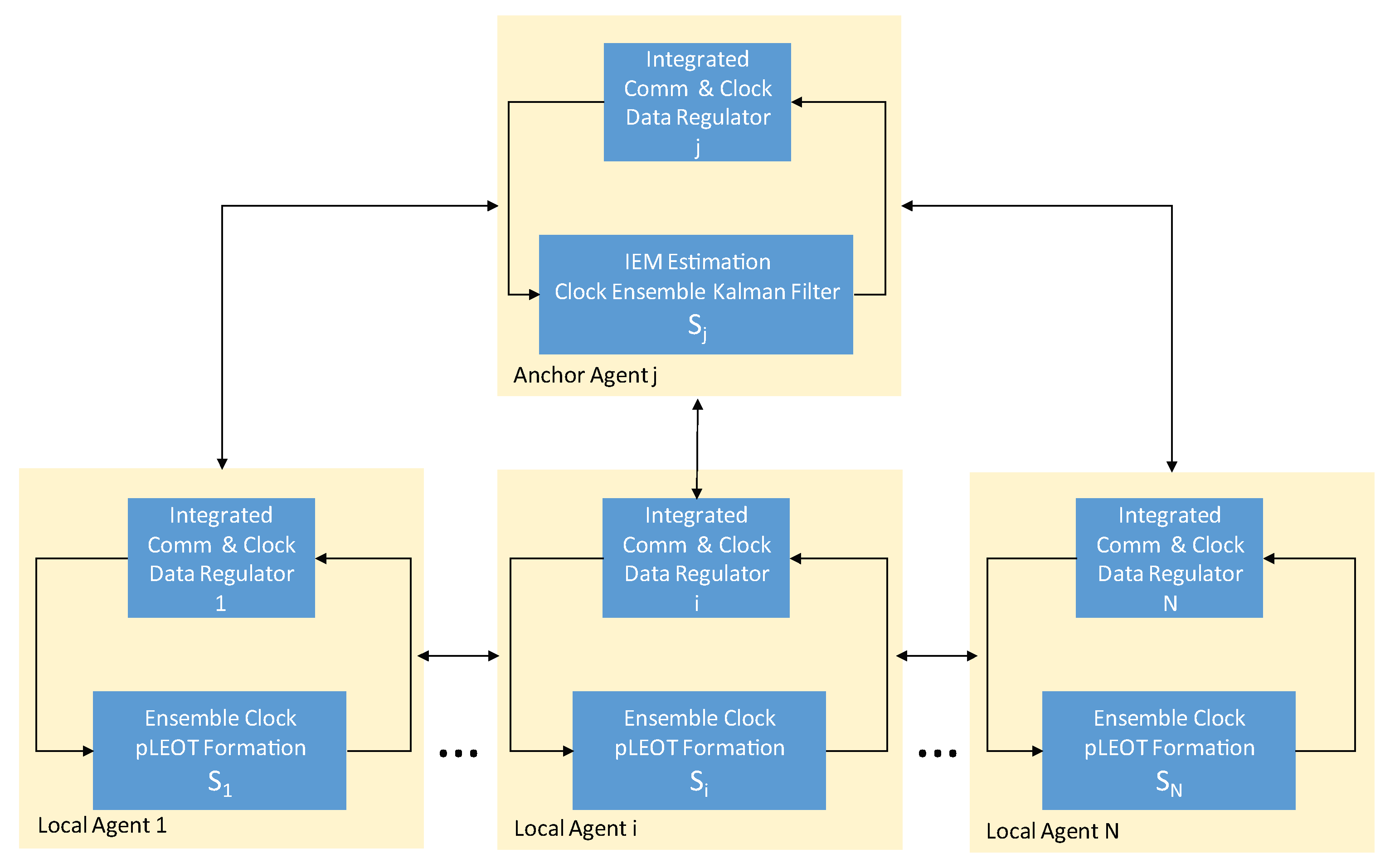
Moreover, the integration of different clock types within a mixed ensemble through a Kalman filter approach is not only feasible but also highly advantageous [16]. This method allows for the creation of a time scale that capitalizes on the unique strengths of each clock, resulting in a composite clock solution that consistently outperforms the best clock in the ensemble [17,18]. As illustrated in Figure 5, an operational architecture is proposed for a pLEOT time scale, applicable to any pLEO constellation. This innovative design maximizes the potential of all participating platforms, existing satellite communications, and inter-satellite measurements, paving the way for effective onboard implementations of pLEOT. Each platform can operate with its local low-noise oscillator, complemented by a numerically controlled oscillator signal synthesis, ensuring exceptional performance and accuracy.

3.1. Independent Physical Clocks Onboard Distributed Platforms

To develop an ensemble time scale for pLEOT, standard state-space models used for modern atomic clocks within a system of N independent physical clocks are considered. As illustrated in [19], one needs to focus on no more than three-state polynomial processes that are driven by white noise. These processes involve the phase, $p_i\left(t\right)$, the frequency, $f_i\left(t\right)$, and the frequency drift, $r_i\left(t\right)$, along with random walk noise processes associated with each clock. Here, i represents the i-th member clock, where i ranges from 1 to N. Consequently, the mathematical representation of each ensemble member clock aboard the orbital platform is defined through these states.

$$\begin{array}{cc}\hfill p_i\left(t_{k+1}\right)& =p_i\left(t_k\right)+\delta f_i\left(t_k\right)+{\displaystyle \frac{{\delta }^2}{2}}{r}_i\left(t_k\right)+{ϵ}_i\left(t_k\right)\hfill \end{array}$$

(30)

$$\begin{array}{cc}\hfill f_i\left(t_{k+1}\right)& =f_i\left(t_k\right)+\delta r_i\left(t_k\right)+{\eta }_i\left(t_k\right)\hfill \end{array}$$

(31)

$$\begin{array}{cc}\hfill r_i\left(t_{k+1}\right)& =r_i\left(t_k\right)+{\alpha }_i\left(t_k\right)\hfill \end{array}$$

(32)

where $t_k$ and $t_{k+1}$ are successive sample times related by the uniform rate $\delta$, e.g.,

$$\begin{array}{c}\hfill t_{k+1}=t_k+\delta .\end{array}$$

(33)

According to Equations (30) through (32), each state of the actual clock, which approximates the behavior of an ideal theoretical clock, evolves from time $t_k$ to the next time $t_{k+1}$ by absorbing a random shock. This shock is driven by aggregate process noise, which consists of three components: ${ϵ}_i\left(t_k\right)$, ${\eta }_i\left(t_k\right)$, and ${\alpha }_i\left(t_k\right)$. Specifically, these correspond to white frequency noise, random walk frequency noise, and random run, respectively. The covariance of the process noise is given by

$$\begin{array}{cc}\hfill Q_i\left(\delta \right)& \triangleq \left[\begin{array}{ccc}{q}_1\delta +{\displaystyle \frac{q_2{\delta }^3}{3}}+{\displaystyle \frac{q_3{\delta }^5}{20}}& {\displaystyle \frac{q_2{\delta }^2}{2}}+{\displaystyle \frac{q_3{\delta }^4}{8}}& {\displaystyle \frac{q_3{\delta }^3}{6}}\\ {\displaystyle \frac{q_2{\delta }^2}{2}}+{\displaystyle \frac{q_3{\delta }^4}{8}}& q_2\delta +{\displaystyle \frac{q_3{\delta }^3}{3}}& {\displaystyle \frac{q_3{\delta }^2}{2}}\\ {\displaystyle \frac{q_3{\delta }^3}{6}}& {\displaystyle \frac{q_3{\delta }^2}{2}}& q_3\delta \end{array}\right],\hfill \end{array}$$

(34)

where the diffusion coefficients ${\sigma }_1$, ${\sigma }_2$, and ${\sigma }_3$ are $q_{\iota }={\sigma }_{\iota }^2$ for $\iota =1,2,3$, thus driving the fundamental noises. Of note, the smaller the process noise covariance of an actual clock, the better the clock’s performance.

3.2. A Theoretical Ideal Clock

As expected, an ideal clock is characterized by the absence of process noise. Specifically, an ideal zeroeth clock, represented by the states $p_0\left(t_k\right)$, $f_0\left(t_k\right)$, and $r_0\left(t_k\right)$, follows the same dynamic model as described in Equations (30)–(32), except that its process noises are set to zero; that is, $q_1^0=q_2^0=q_3^0=0$. As a result, it follows that

$$\begin{array}{c}\hfill Q^0\left(\delta \right)=\left[\begin{array}{ccc}0& 0& 0\\ 0& 0& 0\\ 0& 0& 0\end{array}\right];\left[\begin{array}{c}{ϵ}^0\left(t_k\right)\\ {\eta }^0\left(t_k\right)\\ {\alpha }^0\left(t_k\right)\end{array}\right]=\left[\begin{array}{c}0\\ 0\\ 0\end{array}\right],\forall k.\end{array}$$

(35)

In other words, the physical clock processes could have been seen as deviations from the ideal clock. This view portrays that the essential role of physical clocks is to provide information on the state of any ideal clock.

3.3. Inter-Platform Measurements Enabled by High-Precision Time Synchronization

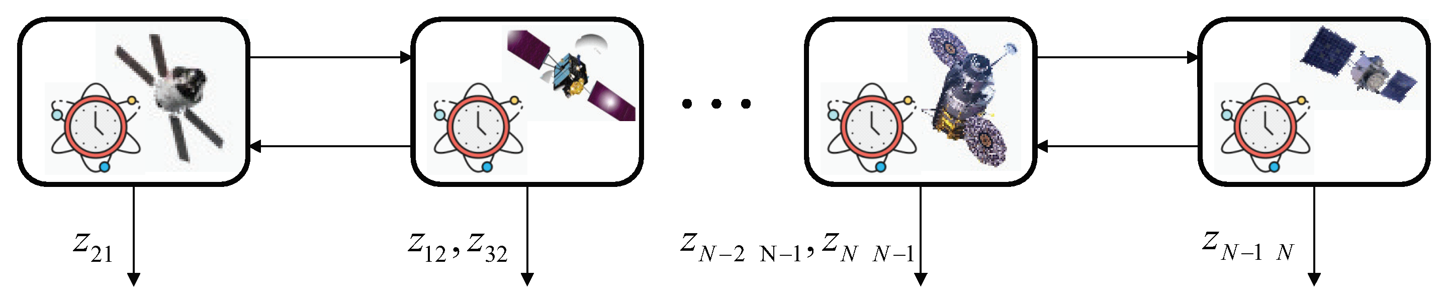
In the framework of the clock ensemble principle with measurements, one begins by comparing the orbiting clocks to one of the ensemble clocks using precise clock-to-clock difference measurements. As illustrated in Figure 6, these measurements are centered on understanding the differences between the initial states of two ensemble clocks. These crucial measurements are activated by events linked to the holdover performance of the physical clocks. They are subsequently processed through a Kalman filter, complemented by a covariance reduction extension to effectively address the unobservability challenge presented by a system of N independent clocks. It is essential to recognize that, in reality, only $N-1$ of these clocks can be independently observed from the measurements obtained.

When implementing a clock ensemble, the inputs to the clock-ensemble Kalman filter are clock-to-clock difference measurements from each bi-directional radio link. For instance, differential phase measurements output from each platform between onboard ith and jth clocks are given by

$$\begin{array}{c}\hfill z_{ij}\left(t_k\right)=p_i\left(t_k\right)-p_j\left(t_k\right)+{\nu }_{ij}\left(t_k\right),\end{array}$$

(36)

where ${\nu }_{ij}\left(t_k\right)$ is a zero-mean Gaussian measurement noise with its covariance adjusted for the behavior of the difference between clocks i and j.

Understanding the complexities of clock measurements is essential as they are significantly influenced by platform dynamics and relativistic effects. A prime example of this is the Sagnac effect, which describes the phase shift that can occur between two measurements taken in opposite directions along the same closed path [20]. In pLEO scenarios, accurately synchronizing time across different platforms requires accounting for the Sagnac effect to ensure precise differential phase measurements.

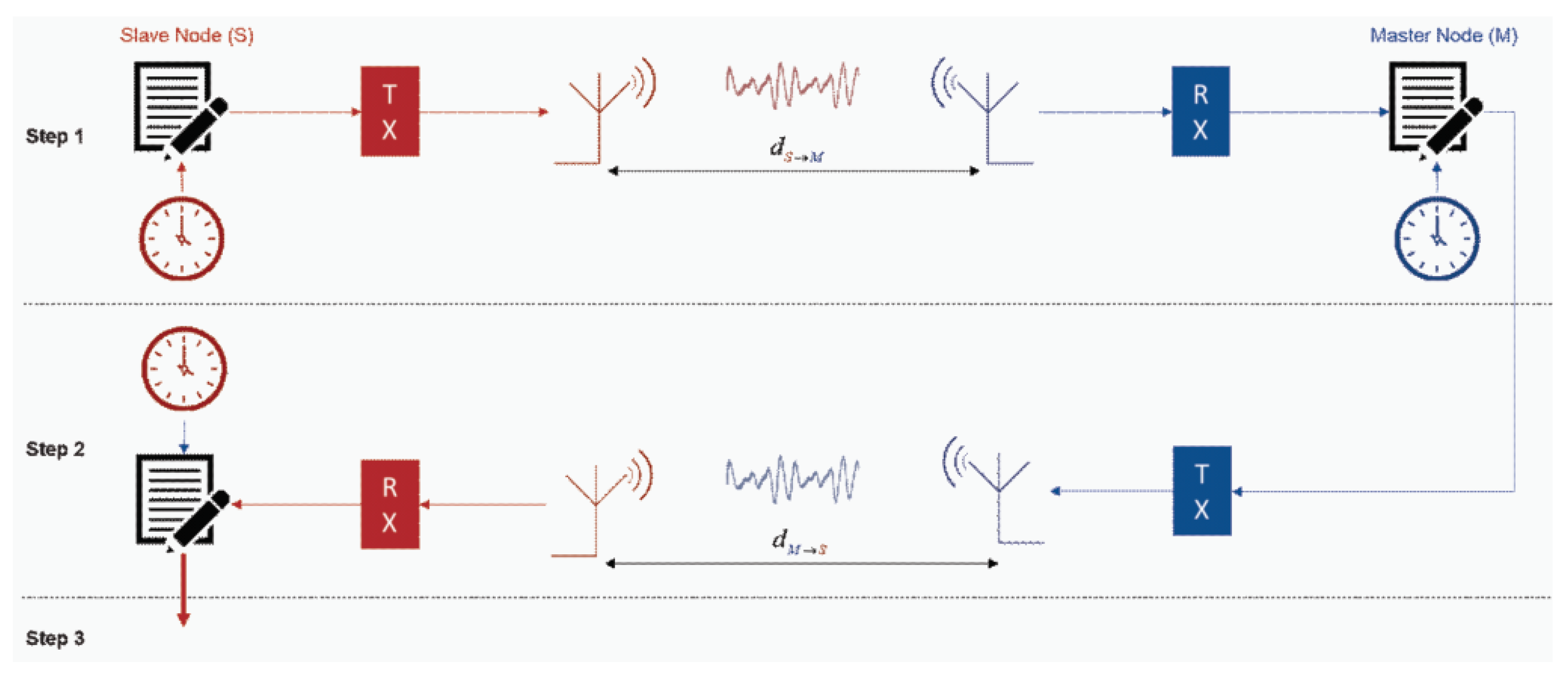
The research presented in [21] introduces an Enhanced Multi-Way Time Transfer (EM-WaTT) solution, which is specifically designed to address the challenges associated with dynamic time coordination. This approach is particularly important when inter-satellite link delays are not uniform across different platforms. As shown in Figure 7, the EM-WaTT method consists of three strategic steps, assuming that the secondary platform, identified as platform j, and the primary platform, referred to as platform i, can exchange timing information through wireless inter-platform communications. By implementing this innovative solution, greater accuracy in time synchronization across various platforms can be achieved.

Step 1. The secondary platform, j, launches its time synchronization protocol by sending a message included with the transmit time stamp, $t_{TX}^S$ to the primary node, i. Upon receiving the message, the primary platform, i, will add the receive timestamp, $t_{RX}^M$ on the primary clock to the message.

Step 2. The primary platform, i, immediately sends the updated message back to the secondary platform, j, which adds the receive time stamp, $t_{RX}^S$ on the secondary clock to the received message.

Step 3. The secondary platform, j, will then perform the clock adjustment based on the updated message, i.e.,

$$\begin{array}{cc}\hfill t_{RX}^M-t_{TX}^S& ={\displaystyle \frac{R_1}{c}}+T_{RX}^M+T_{TX}^S+\Delta t\hfill \end{array}$$

(37)

$$\begin{array}{cc}\hfill t_{RX}^S-t_{TX}^M& ={\displaystyle \frac{R_2}{c}}+T_{TX}^M+T_{RX}^S-\Delta t,\hfill \end{array}$$

(38)

where in this context, $R_1$ and $R_2$ represent the distances between the secondary and primary platforms at the time of transmission, respectively. The terms $T_{TX}^S$ and $T_{RX}^S$ refer to the transmit and receive processing times of the secondary platform j. Similarly, $T_{RX}^M$ and $T_{TX}^M$ indicate the processing times to receive and transmit from the primary platform i. In practical applications, these processing times are fixed based on local signal processing clocks with a limited number of clock cycles. Finally, the speed of the radio wave is represented by the speed of light, denoted as c.

Thus, the clock adjustment, $\Delta t$, at the secondary platform, j, is

$$\begin{array}{cc}\hfill \Delta t& ={\displaystyle \frac{{\widehat{v}}_S·{\widehat{x}}_S(t_{RX}^S-t_{TX}^M-T_{RX}^S+T_{RX}^M)}{2c}}\hfill \\ \hfill & +{\displaystyle \frac{(2t_{RX}^M-t_{TX}^S-t_{RX}^S+T_{TX}^M+T_{RX}^S-T_{RX}^M-T_{TX}^S)}{2}},\hfill \end{array}$$

(39)

where ${\widehat{x}}_S$ and ${\widehat{v}}_S$ are the relative position and velocity vectors of the secondary platform, j, concerning the primary platform, i, which are operated under the dot product of two vectors.

3.4. Generation of Multi-Platform Clock Ensemble

In summary, the main challenge in the time scale problem for an ensemble of separate and independent clocks, such as those used in deployed AltPNT satellite systems, is accurately estimating the states of each clock within the ensemble. Clock-to-clock difference measurements between ensemble members are taken instantly and used to determine each clock’s state relative to a designated reference clock in the system. It is important to note that these reference clocks exhibit random behaviors characterized by non-zero process noise.

Building on the foundational work referenced in [22], several key points are emphasized, particularly regarding the comparison of two participating clocks, denoted as i and j. The objective is typically to estimate the differences in clock states based on the model outlined in Equations (40)–(42), with each measurement representing the difference between the readings of the two cooperating clocks.

$$\begin{array}{cc}\hfill p_{ij}\left(t_{k+1}\right)& =p_{ij}\left(t_k\right)+\delta f_{ij}\left(t_k\right)+{\displaystyle \frac{{\delta }^2}{2}}{r}_{ij}\left(t_k\right)+{ϵ}_{ij}\left(t_k\right)\hfill \end{array}$$

(40)

$$\begin{array}{cc}\hfill f_{ij}\left(t_{k+1}\right)& =f_{ij}\left(t_k\right)+\delta r_{ij}\left(t_k\right)+{\eta }_{ij}\left(t_k\right)\hfill \end{array}$$

(41)

$$\begin{array}{cc}\hfill r_{ij}\left(t_{k+1}\right)& =r_{ij}\left(t_k\right)+{\alpha }_{ij}\left(t_k\right).\hfill \end{array}$$

(42)

3.5. Kalman-Filter Based Clock Ensemble Solution

In linear and Gaussian estimation environments, the estimates and covariances produced by the Kalman filter at time $t_k$ serve as sufficient statistics for the clock system and consider all clock-to-clock measurements up to that point. Figure 8 illustrates an approach for designing a Kalman filter-based clock ensemble.

It is necessary to define a state vector that describes the time-difference states among these onboard timing systems

$$\begin{array}{cc}\hfill x_{ij}\left(t_k\right)& \triangleq \left[\begin{array}{c}{p}_{ij}\left(t_k\right)\\ f_{ij}\left(t_k\right)\\ r_{ij}\left(t_k\right)\end{array}\right].\hfill \end{array}$$

(43)

We also consider the noise vector, $w_{ij}\left(t_k\right)$, that causes the clock states to evolve

$$\begin{array}{cc}\hfill w_{ij}\left(t_k\right)& \triangleq \left[\begin{array}{c}{ϵ}_{ij}\left(t_k\right)\\ {\eta }_{ij}\left(t_k\right)\\ {\alpha }_{ij}\left(t_k\right)\end{array}\right],\hfill \end{array}$$

(44)

and the state transition matrix that depends on the uniform sampling rate, $\delta$, and contains the clock dynamics

$$\begin{array}{cc}\hfill {\Phi }_{\delta }& \triangleq \left[\begin{array}{ccc}1& \delta & {\displaystyle \frac{{\delta }^2}{2}}\\ 0& 1& \delta \\ 0& 0& 1\end{array}\right].\hfill \end{array}$$

(45)

Thus, the basic dynamical system (40)–(42) is now rewritten as

$$\begin{array}{c}\hfill x_{ij}(t_k+1)={\Phi }_{\delta }{x}_{ij}\left(t_k\right)+w_{ij}\left(t_k\right).\end{array}$$

(46)

Notably, the process noise, $w_{ij}(·)$, is Gaussian with zero mean and covariance matrix, $Q_{ij}$

$$\begin{array}{c}\hfill Q_{ij}=E\left\{w_{ij}{w}_{ij}^T\right\},\end{array}$$

(47)

which is the sum of $Q_i\left(\delta \right)$ and $Q_j\left(\delta \right)$, denoted by the process noise covariances for each ensemble clock. The method for computing these process noise covariances from the Allan deviation values associated with an oscillator is detailed in [23].

Furthermore, the error covariance matrix associated with the filtered estimate of $x_{ij}\left(t_k\right)$, ${\widehat{x}}_{ij}\left(t_k\right)$ is given by

$$\begin{array}{c}\hfill P_{ij}\left(t_k\right)=E\left\{[x_{ij}\left(t_k\right)-{\widehat{x}}_{ij}\left(t_k\right)]{[x_{ij}\left(t_k\right)-{\widehat{x}}_{ij}\left(t_k\right)]}^T\right\},\end{array}$$

(48)

which can be computed recursively; just before a measurement and just after a measurement, e.g., $P_{ij}\left(t_k^{-}\right)$ and $P_{ij}\left(t_k^{+}\right)$.

Interestingly enough, the filtered estimate, ${\widehat{x}}_{ij}\left(t_k\right)$ uses information from the measurement equation, e.g.,

$$\begin{array}{c}\hfill z_{ij}\left(t_k\right)=H_{ij}{x}_{ij}\left(t_k\right)+{\nu }_{ij}\left(t_k\right),\end{array}$$

(49)

where $H_{ij}$ is the observation matrix of 1 and ${\nu }_{ij}\left(t_k\right)$ is a Gaussian noise with zero mean and covariance of $R_{ij}$.

Finally, the mean-squared filtered estimator of $x_{ij}\left(t_{k+1}\right)$, ${\widehat{x}}_{ij}\left(t_{k+1}\right)$, written in the predictor-corrector format, is

$$\begin{array}{cc}\hfill {\widehat{x}}_{ij}\left(t_{k+1}\right)& ={\Phi }_{\delta }{\widehat{x}}_{ij}\left(t_k\right)+K_{ij}\left(t_{k+1}\right)[z_{ij}\left(t_{k+1}\right)-H_{ij}{\Phi }_{\delta }{\widehat{x}}_{ij}\left(t_k\right)]\hfill \end{array}$$

(50)

and the Kalman gain, $K_{ij}\left(t_{k+1}\right)$ is specified by the following set of relations

$$\begin{array}{cc}\hfill K_{ij}\left(t_{k+1}\right)& =P_{ij}\left(t_{k+1}^{-}\right)H_{ij}^T{[H_{ij}{P}_{ij}\left(t_{k+1}^{-}\right)H_{ij}^T+R_{ij}]}^{-1}\hfill \end{array}$$

(51)

$$\begin{array}{cc}\hfill P_{ij}\left(t_{k+1}^{+}\right)& =K_{ij}\left(t_{k+1}\right)R_{ij}{K}_{ij}^T\left(t_{k+1}\right)+[I-K_{ij}\left(t_{k+1}\right)H_{ij}]P_{ij}\left(t_{k+1}^{-}\right){[I-K_{ij}\left(t_{k+1}\right)H_{ij}]}^T\hfill \end{array}$$

(52)

$$\begin{array}{cc}\hfill P_{ij}\left(t_{k+1}^{-}\right)& ={\Phi }_{\delta }{P}_{ij}\left(t_k^{+}\right){\Phi }_{\delta }^T+Q_{ij}.\hfill \end{array}$$

(53)

Substituting (46) into (50), the estimate of random shocks is

$$\begin{array}{cc}\hfill {\widehat{w}}_{ij}\left(t_k\right)& ={\widehat{x}}_{ij}\left(t_{k+1}\right)-{\Phi }_{\delta }{\widehat{x}}_{ij}\left(t_k\right)\hfill \end{array}$$

(54)

$$\begin{array}{cc}\hfill & =K_{ij}\left(t_{k+1}\right)[z_{ij}\left(t_{k+1}\right)-H_{ij}{\Phi }_{\delta }{\widehat{x}}_{ij}\left(t_k\right)].\hfill \end{array}$$

(55)

3.6. The Basic Time Scale Equations

In a pLEO constellation, where multiple clocks are present, the effects of clock errors or failures can be detected and mitigated by analyzing the behavior of clock phase discrepancies across the different relative phase measurements. Specifically, after completing the clock difference process for all clocks $j=1,\cdots ,N$ (where $j\ne i$), we can investigate the individual clock phase discrepancies by solving a system of N simultaneous equations for the N phase discrepancies.

$$\begin{array}{cc}\hfill \sum _{i=1}^N{a}_i{\widehat{ϵ}}_i\left(t_k\right)& =0\hfill \\ \hfill {\widehat{ϵ}}_i\left(t_k\right)-{\widehat{ϵ}}_j\left(t_k\right)& =k_{ij}^p\left(t_{k+1}\right)[z_{ij}\left(t_{k+1}\right)-H_{ij}{\Phi }_{\delta }{\widehat{x}}_{ij}\left(t_k\right)].\hfill \end{array}$$

(56)

Thus, it leads to

$$\begin{array}{c}\hfill {\widehat{ϵ}}_j\left(t_k\right)=\sum _{i=1}^N{a}_i{k}_{ij}^p\left(t_{k+1}\right)[H_{ij}{\Phi }_{\delta }{\widehat{x}}_{ij}\left(t_k\right)-z_{ij}\left(t_{k+1}\right)].\end{array}$$

(57)

Now, it should be realized that of all the phase shocks estimated as in (57), the individual clock phases are given by

$$\begin{array}{cc}\hfill {\widehat{p}}_j\left(t_{k+1}\right)& ={\widehat{p}}_j\left(t_k\right)+\delta {\widehat{f}}_j\left(t_k\right)+{\displaystyle \frac{{\delta }^2}{2}}{\widehat{r}}_j\left(t_k\right)+{\widehat{ϵ}}_j\left(t_k\right)\hfill \end{array}$$

(58)

$$\begin{array}{cc}\hfill & ={\widehat{p}}_j\left(t_k\right)+\delta {\widehat{f}}_j\left(t_k\right)+{\displaystyle \frac{{\delta }^2}{2}}{\widehat{r}}_j\left(t_k\right)+\sum _{i=1}^N{a}_i{k}_{ij}^p\left(t_{k+1}\right)[H_{ij}{\Phi }_{\delta }{\widehat{x}}_{ij}\left(t_k\right)-z_{ij}\left(t_{k+1}\right)].\hfill \end{array}$$

(59)

Interestingly, the above result highlights another compelling aspect of the proposed time scale problem: during each iteration, there is inadequate information to determine the phase states of individual clocks, as the prior frequency state, ${\widehat{f}}_j\left(t_k\right)$, and the frequency drift state, ${\widehat{r}}_j\left(t_k\right)$, are unknown. However, as shown in (55), the difference between frequency shocks is known. Therefore, it is essential to estimate the individual frequency shocks for each clock. A similar requirement applies to the individual frequency-drift random shocks for each clock.

It is important to note that there are only $N-1$ simultaneous equations for N unknowns. This ambiguity can be resolved by applying the same assumption about the frequency and frequency drift shocks that was previously made about the phase shocks, as shown in (56)

$$\begin{array}{cc}\hfill \sum _{i=1}^N{b}_i\left(t_k\right){\widehat{\eta }}_i\left(t_k\right)& =0\hfill \end{array}$$

(60)

$$\begin{array}{cc}\hfill \sum _{i=1}^N{c}_i\left(t_k\right){\widehat{\alpha }}_i\left(t_k\right)& =0.\hfill \end{array}$$

(61)

Using the result (55), it is easy to see that both frequency and frequency drift random shocks can be obtained for each clock

$$\begin{array}{cc}\hfill {\widehat{\eta }}_j\left(t_k\right)& =\sum _{i=1}^N{b}_i{k}_{ij}^f\left(t_{k+1}\right)[H_{ij}{\Phi }_{\delta }{\widehat{x}}_{ij}\left(t_k\right)-z_{ij}\left(t_{k+1}\right)]\hfill \end{array}$$

(62)

$$\begin{array}{cc}\hfill {\widehat{\alpha }}_j\left(t_k\right)& =\sum _{i=1}^N{c}_i{k}_{ij}^r\left(t_{k+1}\right)[H_{ij}{\Phi }_{\delta }{\widehat{x}}_{ij}\left(t_k\right)-z_{ij}\left(t_{k+1}\right)].\hfill \end{array}$$

(63)

Consequently, the solutions for frequency and frequency aging can be obtained by inserting the values for the random shocks from Equations (61) and (62) into Equation (46)

$$\begin{array}{cc}\hfill {\widehat{f}}_j\left(t_{k+1}\right)& ={\widehat{f}}_j\left(t_k\right)+\delta {\widehat{r}}_j\left(t_k\right)+\sum _{i=1}^N{b}_i{k}_{ij}^f\left(t_{k+1}\right)[H_{ij}{\Phi }_{\delta }{\widehat{x}}_{ij}\left(t_k\right)-z_{ij}\left(t_{k+1}\right)]\hfill \end{array}$$

(64)

and

$$\begin{array}{cc}\hfill {\widehat{r}}_j\left(t_{k+1}\right)& ={\widehat{r}}_j\left(t_k\right)+\sum _{i=1}^N{c}_i{k}_{ij}^r\left(t_{k+1}\right)[H_{ij}{\Phi }_{\delta }{\widehat{x}}_{ij}\left(t_k\right)-z_{ij}\left(t_{k+1}\right)].\hfill \end{array}$$

(65)

The algorithm for the clock ensemble, as described in Equations (59), (64) and (65), begins with initial values for three states: $p_j\left(t_0\right)$, $f_j\left(t_0\right)$, and $r_j\left(t_0\right)$. For each iteration, the algorithm generates the phase, frequency, and frequency drift states by adjusting the weights associated with these parameters. The weights are set in such a way that they satisfy the limit theorem, which states that the sum of the weighted random shocks approaches zero as the number of clocks increases.

4. pLEO Time Scale Realizations

In the capability concept of a pLEOT time scale within AltPNT, measurements taken between ensemble members are leveraged to accurately estimate the state of each participating clock relative to the theoretical reference known as the implicit ensemble mean (IEM). Furthermore, the Kalman filter provides estimates of the member clocks from the ensemble clock on the anchor platform, which can be shared with all participating orbital platforms. While there are various methods to achieve this, the simplest and most effective approach is to periodically transmit the clock state estimates determined by the Kalman filter to these platforms. By doing so, each platform receiving timing signals from its physical clock can utilize these estimates to adjust its corrected clock. As a result, this data-driven correction leads to a more stable timing signal compared to that of a free-running physical clock, enhancing overall performance and reliability.

4.1. Implicit Ensemble Mean (IEM)

Given the foregoing, at any time $t_k$, the implicit ensemble mean $\overline{x_0}|X\left(t_k\right)$ and $X\left(t_k\right)\triangleq \{x_1\left(t_k\right),x_2\left(t_k\right),\cdots ,x_N\left(t_k\right)\}$ is defined as the conditional mean of the ideal clock state $x_0\left(t_k\right)$ or in vector form of

$$\begin{array}{c}\hfill x_0\left(t_k\right)\triangleq \left[\begin{array}{c}{p}_0\left(t_k\right)\\ f_0\left(t_k\right)\\ r_0\left(t_k\right)\end{array}\right]\end{array}$$

(66)

given any i-th physical clock state $x_i\left(t_k\right)$ where

$$\begin{array}{c}\hfill x_i\left(t_k\right)\triangleq \left[\begin{array}{c}{p}_i\left(t_k\right)\\ f_i\left(t_k\right)\\ r_i\left(t_k\right)\end{array}\right]\end{array}$$

(67)

and $i=1,\cdots ,N$ of all real member clocks, given all the available clock difference measurements up to time $t_k$, and given no prior information on the ideal clock.

According to the definition of the ideal clock presented in Section 2, we can define the bias state for each ensemble clock as the difference $b_i\left(t_k\right)$ between the physical clock state $x_i\left(t_k\right)$ and that of the ideal clock. For example, this bias state represents how much each member clock deviates from the ideal clock’s time

$$\begin{array}{c}\hfill x_i\left(t_k\right)=x_0\left(t_k\right)+b_i\left(t_k\right),\end{array}$$

(68)

which leads to

$$\begin{array}{c}\hfill x_i\left(t_k\right)=x_0\left(t_k\right)+{\widehat{x}}_i\left(t_k\right)+e_i\left(t_k\right),\end{array}$$

(69)

where $e_i\left(t_k\right)$ are the errors in the estimate ${\widehat{x}}_i\left(t_k\right)$, i.e.,

$$\begin{array}{c}\hfill {\widehat{x}}_i\left(t_k\right)\triangleq \left[\begin{array}{c}{\widehat{p}}_i\left(t_k\right)\\ {\widehat{f}}_i\left(t_k\right)\\ {\widehat{r}}_i\left(t_k\right)\end{array}\right]\end{array}$$

(70)

as governed by (59), (64) and (65) of the bias $b_i\left(t_k\right)$.

In estimation theory, the IEM estimation is expressed as the conditional mean of $x_0\left(t_k\right)$. However, this value is not computed explicitly because it relies on all the physical clock states $X\left(t_k\right)$, which are often difficult to obtain from a single orbital platform in the pLEO clock system. Nevertheless, any i-th corrected clock can be made accessible to its participating orbital platform, subject to certain limitations of inter-satellite links. Essentially, any physical clock that has been corrected for its estimated bias can serve as a reliable representation of the IEM estimation with high accuracy, for example, in practical applications

$$\begin{array}{c}\hfill {\overline{x}}_0\left(t_k\right)|X\left(t_k\right)=x_i\left(t_k\right)-{\widehat{x}}_i\left(t_k\right).\end{array}$$

(71)

4.2. Principle of IEM Formations

In the innovative time scale concept for AltPNT, each onboard orbital platform i (where $i=1,\dots ,N$) is designed to incorporate a clock ensemble for pLEOT, moving beyond reliance on a single precision clock. As depicted in Figure 9, to ensure accurate time output from this clock ensemble, an oven-controlled quartz oscillator (OCXO) is meticulously calibrated using a micro-phase stepper (MPS) on every platform. This strategic setup is crucial because, with all platforms interconnected, just one connection to GPS or a single ground station is sufficient to accurately calculate the offset of pLEOT relative to GPST or UTC. This approach not only enhances precision but also optimizes connectivity and reliability across the system.

In relation to the realization of the IEM, an anchor platform continuously collects clock-to-clock difference measurement data. These data are processed using a clock-ensemble Kalman filter for each ensemble member clock. The output of this filter, as indicated in Equation (69), provides the estimate of the i-th clock state. This estimate is expressed as the difference between the physical clock state $x_i\left(t_k\right)$ and the IEM of $x_0\left(t_k\right)$, along with the estimation noise $e_i\left(t_k\right)$. Additionally, the measurement of the MPS of the steerable OCXO, denoted as $x_{i,OCXO}\left(t_k\right)$, is also important. This measurement describes the local difference between the two clock states $x_i\left(t_k\right)$ and $x_{i,OCXO}\left(t_k\right)$

$$\begin{array}{c}\hfill z_{i,OCXO}\left(t_k\right)=x_{i,OCXO}\left(t_k\right)-x_i\left(t_k\right)+v_i\left(t_k\right).\end{array}$$

(72)

Next, the estimate for the free-running clock, ${\widehat{x}}_i\left(t_k\right)$, is combined with the measurement, $z_{i,OCXO}\left(t_k\right)$, thus resulting in the difference measurement between the OCXO and the IEM, disturbed by the estimation and measurement errors

$$\begin{array}{cc}\hfill {\widehat{x}}_i\left(t_k\right)+z_{i,OCXO}\left(t_k\right)& =x_{i,OCXO}\left(t_k\right)-x_0\left(t_k\right)-e_i\left(t_k\right)+v_i\left(t_k\right).\hfill \end{array}$$

(73)

4.3. Onboard Steering OCXO to IEM

The realization of the IEM time scale generated by the clock-ensemble Kalman filter involves locking a physical oscillator to the IEM. Consequently, the MPS output from an OCXO onboard the pLEO platform i (for $i=1,\cdots ,N$) adheres to the IEM and thus serves as a realization of it. The control value applied by the MPS is derived using various steering techniques [24].

In real measurements, only the clock-to-clock difference measurement is directly available. Therefore, it is possible to simulate this situation by propagating and estimating the difference between the OCXO and IEM clocks for the i-th onboard platform (where $i=1,\cdots ,N$). This is achieved using the two-state clock model (46), which describes the behavior of the difference between two participating clocks

$$\begin{array}{cc}\hfill s_i\left(t_k\right)& =x_{i,OCXO}\left(t_k\right)-x_0\left(t_k\right)\hfill \end{array}$$

(74)

$$\begin{array}{cc}\hfill s_i\left(t_{k+1}\right)& =A_i\left(h\right)s_i\left(t_k\right)+{\nu }_i\left(t_k\right),\hfill \end{array}$$

(75)

where the process noise, ${\nu }_i\left(t_k\right)$ is a zero-mean Gaussian with its covariance, $Q_{{\nu }_i}\left(h\right)$ taken into account of the behaviors of the OCXO and IEM, i.e., $Q_{{\nu }_i}=Q_{OCXO}\left(h\right)+Q_{IEM}\left(h\right)$. The transition matrix on the differential clock state, $s_i\left(t_k\right)$, is described by

$$\begin{array}{c}\hfill A_i\left(h\right)=\left[\begin{array}{cc}1& h\\ 0& 1\end{array}\right]\end{array}$$

(76)

and $t_{k+1}-t_k=h$ is the control interval which is one of the few parameters used to tune the steered signal response corresponding to the target state errors. Intuitively, the impact of the control rates will influence the stability of the OCXO reference clock on each orbital platform.

If repeated adjustment of oscillator frequency, called clock steering, is applied in the realization of IEM to take advantage of the best clock stability across different averaging intervals, the differential clock model (75) onboard each platform i and $i=1,\cdots ,N$ will then need to be extended by the control term $B_i\left(h\right)u_i\left(t_k\right)$ as follows:

$$\begin{array}{c}\hfill s_i\left(t_{k+1}\right)=A_i\left(h\right)s_i\left(t_k\right)+B_i\left(h\right)u_i\left(t_k\right)+{\nu }_i\left(t_k\right)\end{array}$$

(77)

with

$$\begin{array}{c}\hfill B_i\left(h\right)=\left[\begin{array}{c}h\\ 1\end{array}\right].\end{array}$$

(78)

Notably, the controllability matrix, $C_i\left(h\right)$, associated with the differential clock model (77) onboard the i-th platform is given by

$$\begin{array}{c}\hfill C_i\left(h\right)=\left[\begin{array}{cc}{B}_i\left(h\right)& A_i\left(h\right)B_i\left(h\right)\end{array}\right]=\left[\begin{array}{cc}h& 2h\\ 1& 1\end{array}\right].\end{array}$$

(79)

And its determinant satisfies $det\left\{C_i\left(h\right)\right\}=-h\ne 0$. Thus, $C_i\left(h\right)$ has full rank for any $h\in {\Re }^{+}$.

It is also important to note that the independence of the selected control interval h on each orbital platform i means that the clock estimates from the Kalman-filter clock ensemble running on the anchor orbital platform j (where $j\ne i$) are distributed to all participating orbital platforms in the network. This distribution occurs at a frequency that differs from the control values $u_i\left(t_k\right)$, which are applied to the MPS of the OCXO oscillator onboard orbital platform i. As a result, the control gains for $u_i\left(t_k\right)$ need to be adjusted to reflect the difference between the control interval, or the communication period h between the anchor orbital platform and the participating orbital platforms, and the filter iteration $\delta$, as discussed in Section 2.

5. Networked Control Systems with Minimal Attention

As highlighted in the previous section, the clock-ensemble Kalman filter operates on a discrete time interval of $\delta$ seconds. Every $\delta$ seconds, the clock-to-clock difference data between the onboard OCXO platform i and the IEM is recorded and transmitted to all participating platforms i (where $i=1,\cdots ,N$). The onboard steering control value is then calculated and applied to the MPS as soon as the user-defined control interval is achieved.

In this framework, reducing bandwidth is essential, particularly by leveraging existing inter-satellite radio links in the fully connected pLEO constellation. This method facilitates the efficient transfer of clock estimates from the clock-ensemble Kalman filter on the anchor platform j to all other participating platforms. This research critically examines how diminishing the number of data packet exchanges, represented as ${\widehat{x}}_i\left(t_k\right)$, between the remote sensor (the clock-ensemble Kalman filter on the anchor platform j) and the steering controller or actuator linked to the local IEM realization on platform i, can enhance overall performance.

The local IEM realization aboard orbital platform i applies its model knowledge in its steering controller or actuator to effectively approximate the OCXO’s behavior concerning the IEM, particularly during intervals when clock estimates from the remote sensor are not available. The core goal is to ensure feedback by updating the state $s_i\left(t_k\right)$ of the local IEM model, as governed by Equation (77), using the actual state $x_i\left(t_k\right)$ of the ensemble clock i. This crucial state information comes from the remote sensor, which is the clock-ensemble Kalman filter operating on anchor orbital platform j.

$$\begin{array}{c}\hfill x_i\left(t_k\right)={\widehat{x}}_i\left(t_k\right)+z_{i,OCXO}\left(t_k\right),\end{array}$$

(80)

which, in accordance with (73), leads to

$$\begin{array}{c}\hfill x_i\left(t_k\right)=x_{i,OCXO}\left(t_k\right)-x_0\left(t_k\right)-e_i\left(t_k\right)+v_i\left(t_k\right).\end{array}$$

(81)

During the remainder of the control interval, the steering action relies on the local IEM realization model onboard orbital platform i. The dynamics of this local IEM model are integrated into the steering controller or actuator, resulting in an open-loop operation for a duration of h seconds.

This research presents an initial step toward developing onboard timing architectures in AltPNT. The analysis explores the trade-off between open-loop and closed-loop steering controls, which could facilitate local pLEOT formation across a pLEO constellation, thereby offering potential resilient navigation services. Interestingly, networked control systems have proven to be invaluable for designing control systems that manage steering frequency standards with minimal oversight and resource allocation.

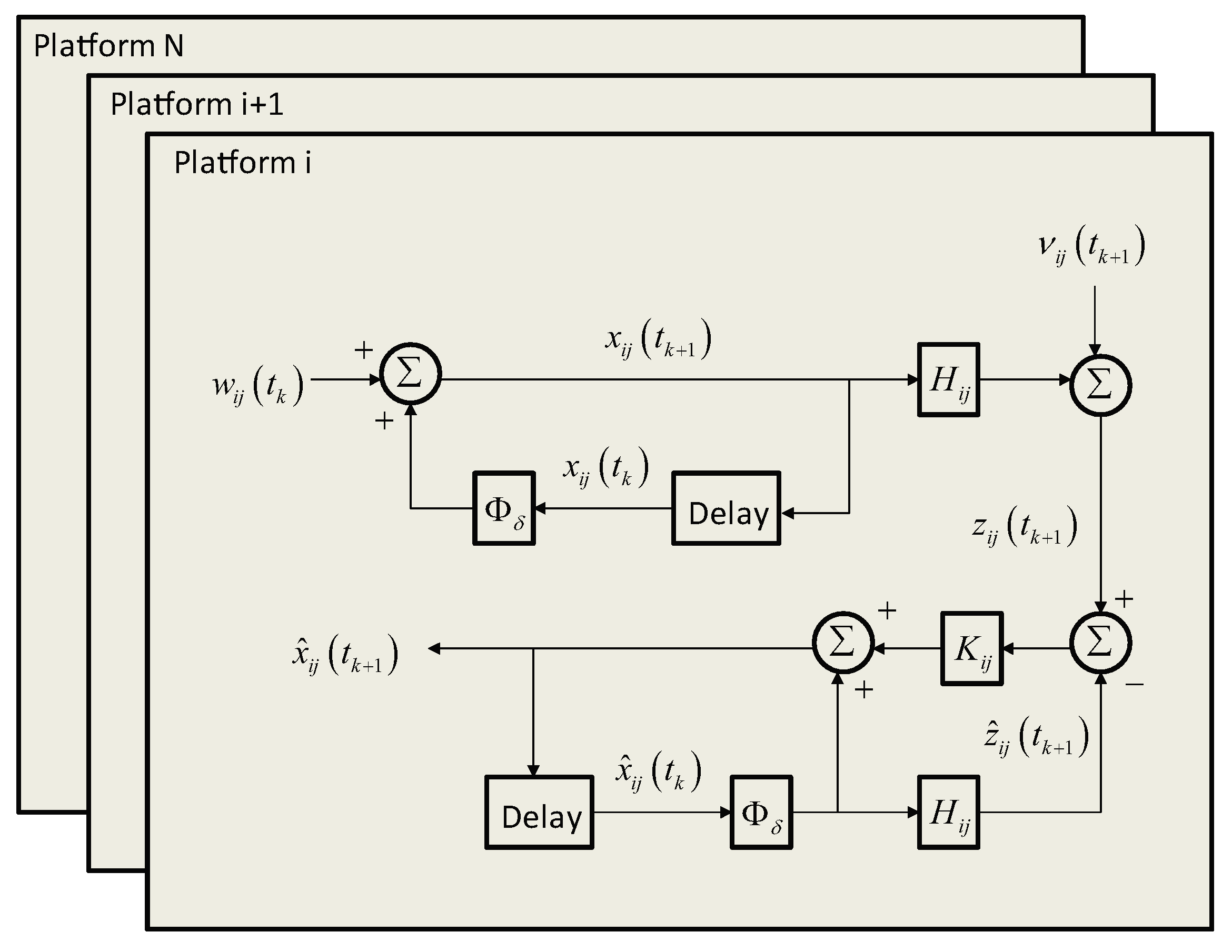
Consider a feedback networked control system in Figure 10, where the actual behavior of the IEM estimate is described by

$$\begin{array}{c}\hfill {\widehat{x}}_i\left(t_{k+1}\right)=A_i\left(\delta \right){\widehat{x}}_i\left(t_k\right)+B_i\left(\delta \right)u_i\left(t_k\right)+w_i\left(t_k\right)),\end{array}$$

(82)

where $B_i\left(\delta \right)=0$ and the update time $t_k$ with $t_{k+1}-t_k=h$ for all k.

Also, the local IEM realization model is given by

$$\begin{array}{c}\hfill s_i\left(t_{k+1}\right)=A_i\left(h\right)s_i\left(t_k\right)+B_i\left(h\right)u_i\left(t_k\right)+{\nu }_i\left(t_k\right).\end{array}$$

(83)

As shown in Figure 10, the remote sensor onboard platform j has the full state, ${\widehat{x}}_i\left(t_k\right)$ available. It will send the state information through the inter-satellite radio links every h seconds.

Finally, the onboard controller, $u_i\left(t_k\right)$ for clock steering by

$$\begin{array}{c}\hfill u_i\left(t_k\right)=K_i{s}_i\left(t_k\right),\end{array}$$

(84)

where one further observes that the gain matrix, $K_i$ affects how quickly the signal transitions from the free-running behavior of the local OCXO clock to the IEM estimate.

The state error, $e_i\left(t_k\right)$ is defined as

$$\begin{array}{c}\hfill e_i\left(t_k\right)={\widehat{x}}_i\left(t_k\right)-s_i\left(t_k\right).\end{array}$$

(85)

The following analysis is motivated by the work [25]. For each index i where $i=1,\dots ,N$, the state error $e_i\left(t_k\right)$ represents the difference between the OCXO state and the IEM. The modeling error matrices, ${\tilde{A}}_i=A_i\left(\delta \right)-A_i\left(h\right)$ and ${\tilde{B}}_i=B_i\left(\delta \right)-B_i\left(h\right)$, indicate the difference between the actual clock of the ensemble member and its corresponding remote IEM realization model.

It is important to note that the local IEM realization model for each index i is updated every h seconds, which means that $e_i\left(t_k\right)=0$ for $k=0,1,\cdots$. This resetting of the state error at each update interval is a crucial feature of the networked control platforms discussed here. Furthermore, it can be demonstrated that the dynamics of the local IEM realization system for index i in the time interval $t\in (t_k,t_{k+1})$ can be described by

$$\begin{array}{c}\hfill y_i\left(t_{k+1}\right)={\Lambda }_i{y}_i\left(t_k\right),\end{array}$$

(86)

where

$$\begin{array}{cc}\hfill {\Lambda }_i& =\left[\begin{array}{cc}{A}_i\left(\delta \right)+B_i\left(\delta \right)K_i& -B_i\left(\delta \right)K_i\\ {\tilde{A}}_i+{\tilde{B}}_i{K}_i& A_i\left(h\right)-{\tilde{B}}_i{K}_i\end{array}\right]\hfill \end{array}$$

(87)

$$\begin{array}{cc}\hfill y_i\left(t_k\right)& =\left[\begin{array}{c}{\widehat{x}}_i\left(t_k\right)\\ e_i\left(t_k\right)\end{array}\right].\hfill \end{array}$$

(88)

Moreover, the discrete state-feedback system (86) is globally exponentially stable around the solution

$$\begin{array}{c}\hfill y_i=\left[\begin{array}{c}{\widehat{x}}_i\\ e_i\end{array}\right]=\left[\begin{array}{c}0\\ 0\end{array}\right]\end{array}$$

(89)

if and only if the eigenvalues of

$$\begin{array}{c}\hfill M_D=\left[\begin{array}{cc}I& 0\\ 0& 0\end{array}\right]{\Lambda }_i\left[\begin{array}{cc}I& 0\\ 0& 0\end{array}\right]\end{array}$$

(90)

are inside the unit circle. The essential implication of results (89) and (90) relates to the necessary and sufficient conditions for the stability of system (86). This outcome specifies the maximum transfer time or the minimum frequency for updating the state in the remote steering controller, denoted as i, associated with the separate orbital platform i, where $i=1,\cdots ,N$. Specifically, it establishes an upper bound for h, referred to as the update time for its local reference time scale, pLEOT i, which is aligned with the global IEM time scale operating on the anchor orbital platform j.

6. Onboard Steering Commands via Minimal-Cost-Variance Control

Each pLEO platform is presumably working to generate its own local IEM realization for pLEOT. To achieve this, each platform will adjust its local reference clock, such as an autonomous robust time scale defined by $pLEOT\left(i\right)$, in relation to the IEM estimation. Alongside the controller update rate, denoted as h, there is an additional tuning parameter called the controller gain, $K_i$. This gain is used to adjust the corresponding OCXO signal response to match the IEM estimate.

In general, a larger controller gain is expected to produce larger frequency corrections for any given offset of the OCXO from the IEM estimate, leading to a more accurate realization of the IEM. To optimize this responsiveness, the elements of the controller gain, $K_i$, which dictate how effectively the autonomous remote time scale system operates on platform i, are designed.

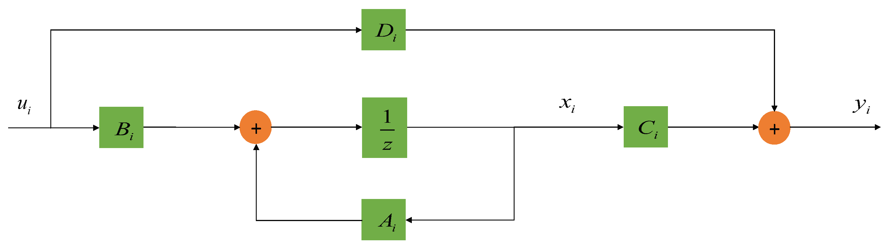
Recall that the discrete-time state-space counterpart of a local IEM realization model (83) that is completely controllable is governed by

$$\begin{array}{cc}\hfill s_i(k+1)& =A_i\left(h\right)s_i\left(k\right)+B_i\left(h\right)u_i\left(k\right)+w_i\left(k\right),\hfill \end{array}$$

(91)

$$\begin{array}{cc}\hfill z_i\left(k\right)& =s_i\left(k\right),\hfill \end{array}$$

(92)

where the states of the steering control system (91) include the phase and frequency of the steered OCXO clock onboard orbital platform i. The steering commands, denoted as $u_i\left(k\right)$, are sent to an actuator such as an MPS device. The output signals or measurements typically consist of the phase deviation $z_i\left(k\right)$ between the local OCXO oscillator and the IEM estimation. The controller $u_i\left(k\right)$ operates on the actuator to minimize the phase deviation $z_i\left(k\right)$. Noise parameters associated with both the OCXO and IEM clocks are determined based on measured Allan deviation curves. The realization of these noises is represented by a zero-mean Gaussian process noise $w_i\left(k\right)$, with its covariance matrix given by $Q_{w_i}\left(h\right)=Q_{i,OCXO}\left(h\right)+Q_{IEM}\left(h\right)$.

Moreover, one of several requirements can be established for clock steering on each platform in relation to the IEM estimation. For instance, the performance indicator suggests a convex cost function for selecting a steering policy. This insight can be represented by a quadratic cost function, based on the idea that the relative penalties assigned to phase and frequency deviations, as well as steering efforts concerning a local reference clock i, can be optimized over a finite horizon, $[n_0,N_i]$, for all time k. To be credible, these penalties must be responsive to the clock steering operations aimed at reducing phase and frequency deviations toward zero

$$\begin{array}{cc}\hfill J_i\left(n_0\right)& =\sum _{k=n_0+1}^{N_i}{L}_i(k,s_i\left(k\right),u_i(k-1))\hfill \end{array}$$

(93)

$$\begin{array}{cc}\hfill & =\sum _{k=n_0+1}^{N_i}[s_i^T\left(k\right)Q_i(k-1)s_i\left(k\right)+u_i^T(k-1)R_i(k-1)u_i(k-1)]\hfill \end{array}$$

(94)

where the weighting coefficients associated with the steering efforts, $R_i(k-1)$ and the phase and frequency deviations, $Q_i(k-1)$ are positive and bounded. In general, if $R_i$ is large compared to $Q_i$, the penalty is large for the controller and/or actuator attempting to drive both phase and frequency deviations toward zero to rapidly. On the other hand, if $Q_i$ is large compared to $R_i$, the controller faces a small penalty for a large steering effort, and the system is driven toward zero more quickly.

The risk management perspective of clock steering operations emphasizes the importance of effective risk handling. It specifically focuses on the feedback steering mechanism that shapes the probability distribution function of the chi-squared random variable referenced in Equation (94). This approach is crucial for ensuring the robustness and reliability of steering operations.

The author has delved into various cost-cumulant control strategies, introducing a risk-value aware performance index defined as a linear manifold composed of a finite set of centralized moments linked to the performance measure affected by a chi-squared random variable. These innovative control strategies provide a transparent framework for effectively allocating performance robustness and reliability requirements across diverse qualitative performance attributes and their corresponding risks, ensuring enhanced decision-making and risk management.

Indeed, the effectiveness of cost-cumulant control algorithms was demonstrated in various applications, such as cable-stayed bridges [26], structures affected by wind [27], and buildings subjected to earthquake vibrations [28]. The results from these implementations were compared to those obtained using Linear-Quadratic-Gaussian (LQG) control, which focuses on minimizing the statistical average of (94). The findings revealed that the cost-cumulant controllers significantly outperformed the results achieved with LQG control.

In light of recent advancements and the growing efficiency of edge computing onboard each orbital platform i, it is both prudent and beneficial to reassess a notable member of the cost-cumulant control family: the minimal-cost-variance (MCV) control. This innovative approach prioritizes the reduction of cost variance while ensuring the cost mean remains within established limits [29]. The MCV control technique is particularly relevant in addressing the escalating concerns surrounding clock steering operations, which play a vital role in maintaining precision and reliability in local reference time scales across diverse orbital platforms. Embracing this technique could significantly enhance the operational frameworks and outcomes.

A highly effective strategy for designers is to set rigorous metrological requirements that enable the clock to be adjusted just once, eliminating the need for repeated actions. This operational requirement for clock adjustment makes the MCV control paradigm an ideal choice for implementing changes to the clock and time scale. By adopting this framework, designers can focus on minimizing the variance of the performance measure, as highlighted in (94), while ensuring that the expected value of that performance measure remains within specified constraints. This approach not only enhances precision but also streamlines efficiency in time management.

As a guide for the reader, this section serves as an important signpost related to the theory of MCV control. It lays the foundation for designing new steering control laws that can achieve the objectives for autonomous, resilient, and remote timing systems. This is accomplished by influencing the probability distribution of the performance measure to accurately estimate IEM parameters in desirable ways. Specifically, the focus on minimizing the variance of $J_i\left(n_0\right)$ while keeping its mean within a defined constraint is relevant to the current context

$$\begin{array}{c}\hfill E\left\{J_i^2\right|Z_i\left(n_0\right)\}-E^2\left\{J_i\left(n_0\right)\right|Z_i\left(n_0\right)\}\end{array}$$

(95)

is minimized, while

$$\begin{array}{c}\hfill E\left\{J_i\left(n_0\right)\right|Z_i\left(n_0\right)\}=h_i(n_0,Z_i\left(n_0\right))\end{array}$$

(96)

where $E\{·|·\}$ denotes the conditional expectation operator and the actual data $Z_i\left(k\right)\triangleq \{z_i\left(n_0\right),z_i(n_0+1),\cdots ,z_i\left(k\right);u_i\left(n_0\right),u_i(n_0+1),\cdots ,u_i(k-1)\}$ measured from local frequency standards onboard separate orbital platforms with $Z_i\left(n_0\right)\triangleq z_i\left(n_0\right)$ and $n_0<k$.

The primary focus of $h_i(n_0,Z_i\left(n_0\right))$ involves practical considerations, such as the desired response, acceptable deviations from that response, and the complexity of the clock steering controller. How should we move forward based on this general assessment? It becomes evident that the choice of $h_i(n_0,Z_i\left(n_0\right))$ is not entirely arbitrary. It must be selected in a way that ensures it is always greater than the following lower bound, i.e.,

$$\begin{array}{c}\hfill \underset{u_i\left(n_0\right),\cdots ,u_i(N_i-1)}{inf}E\left\{J_i\left(n_0\right)\right|Z_i\left(n_0\right)\}.\end{array}$$

(97)

At this moment, it may be shown that for the special class of the linear-quadratic problem, the mean value constraint is intuitively given by

$$\begin{array}{c}\hfill h_i(n_0,Z_i\left(n_0\right))=m_i\left(n_0\right)+s_i^T\left(n_0\right)M_i\left(n_0\right)s_i\left(n_0\right)\end{array}$$

(98)

where $m_i\left(n_0\right)\in {\mathbb{R}}^{+}$ and $M_i\left(n_0\right)$ is a symmetric and nonnegative matrix. Moreover, both $m_i\left(n_0\right)$ and $M_i\left(n_0\right)$ should be selected such that

$$\begin{array}{c}\hfill h_i(n_0,Z_i\left(n_0\right))>{\alpha }_i(n_0,Z_i\left(n_0\right))\end{array}$$

(99)

where ${\alpha }_i(n_0,Z_i\left(n_0\right))$ is as given by (97).

Notably, a recursion equation for the optimal variance cost involves the standard procedure for this type of problem. First, the constraint equation is combined with the expression to be minimized using a Lagrange multiplier, ${\mu }_i\left(n_0\right)$. The resulting equation is then incorporated into a broader class of problems where $n_0$ is treated as a variable rather than a fixed initial time. Solving this more general problem leads straightforwardly to the solution of the specific problem at hand. Therefore, the goal is to determine ${\mu }_i\left(k\right)$, and the clock steering policy should take the form ${⋎}_i\left(k\right)\triangleq {⋎}_i(k,Z_i\left(k\right))$, for $n_0\le k\le N_i-1$, e.g.,

$$\begin{array}{c}\hfill E\left\{J_i^2\left(k\right)|Z_i\left(k\right)\right\}-E^2\left\{J_i\left(k\right)|Z_i\left(k\right)\right\}+4{\mu }_i\left(k\right)\left[E\left\{J_i\left(k\right)\right|Z_i\left(k\right)\}-h_i(k,Z_i\left(k\right))\right]\end{array}$$

(100)

is minimized, In this context, let ${\mu }_i\left(k\right)\in {\mathbb{R}}^{+}$ represent a Lagrange multiplier. The four pre-multiplying ${\mu }_i\left(k\right)$ values have been introduced for convenience. It is important to note that $Z_i\left(k\right)$ encompasses all the information necessary for clock and time scale adjustments at time k. The chosen form for ${⋎}_i\left(k\right)$, along with the requirement for boundedness, contributes to defining the class of admissible steering controls.

Before proceeding with the development of the recursion equation, however, let ${⋎}_i^k\triangleq \{{⋎}_i\left(k\right),{⋎}_i(k+1),\cdots ,{⋎}_i(N_i-1)\}$, $k=n_0,\cdots ,N_i$, and let

$$\begin{array}{c}V{C}_i(k,Z_i\left(k\right)|{⋎}_i^k)=\hfill \\ \hfill E\left\{J_i^2\left(k\right)|Z_i\left(k\right)\right\}-E^2\left\{J_i\left(k\right)\right|Z_i\left(k\right)\}+4{\mu }_i\left(k\right)\left[E\left\{J_i\left(k\right)\right|Z_i\left(k\right)\}-h_i(k,Z_i\left(k\right))\right]\end{array}$$

(101)

where $V{C}_i$ signifies “variance cost”.

To prevent mathematical details from overshadowing the concepts being analyzed, some steps leading to the recursion equation for the variance cost have been referenced in [29]. At this point, the assumption of linear control laws naturally leads to optimal quadratic costs. In other words, when using linear control laws, it is always possible to express the costs in this way

$$\begin{array}{c}\hfill V{C}_i^{*}(k+1,Z_i(k+1))=v_i^{*}(k+1)+s_i^T(k+1)V_i^{*}(k+1)s_i(k+1)\end{array}$$

(102)

where $v_i^{*}(k+1)\in {\mathbb{R}}^{+}$ and $V_i^{*}(k+1)$ are symmetric and nonnegative real-valued matrices and whereas $n_0\le k\le N_i-1$. Thus, for ${\beta }_i\left(k\right)\triangleq A_i\left(h\right)s_i\left(k\right)+B_i\left(h\right){⋎}_i\left(k\right)$, it follows that

$$\begin{array}{cc}\hfill E\left\{V{C}_i^{*}(k+1,Z_i(k+1))\right|Z_i\left(k\right)\}& =v_i^{*}(k+1)\hfill \\ \hfill & +{\beta }_i^T\left(k\right)V_i^{*}(k+1){\beta }_i\left(k\right)+Tr\left\{V_i^{*}(k+1)Q_{w_i}\right\}.\hfill \end{array}$$

(103)

Aside from the relevance of $S_i\left(k\right)\triangleq Q_i\left(k\right)+M_i(k+1)$ for $n_0\le k\le N_i-1$, to the terminal conditions given by $m_i\left(N_i\right)=0$, $M_i\left(N_i\right)=0$, $v_i^{*}\left(N_i\right)=0$, and $V_i^{*}\left(N_i\right)=0$, some mathematical manipulations further yield

$$\begin{array}{cc}\hfill & V{C}_i^{*}(k,Z_i\left(k\right))=\underset{{⋎}_i\left(k\right),{\mu }_i\left(k\right)}{min}\{4{\beta }_i^T\left(k\right)S_i\left(k\right)Q_{w_i}{S}_i\left(k\right){\beta }_i\left(k\right)+E\left\{w_i^T\left(k\right)S_i\left(k\right)w_i\left(k\right)\right\}\hfill \\ \hfill & -T{r}^2\left\{S_i\left(k\right)Q_{w_i}\right\}+v_i^{*}(k+1)+{\beta }_i^T\left(k\right)V_i^{*}(k+1){\beta }_i\left(k\right)+Tr\left\{V_i^{*}(k+1)Q_{w_i}\right\}+4{\mu }_i\left(k\right)[m_i(k+1)\hfill \\ \hfill & +{⋎}_i^T\left(k\right)R_i\left(k\right){⋎}_i\left(k\right)+{\beta }_i^T\left(k\right)S_i\left(k\right){\beta }_i\left(k\right)+Tr\left\{S_i\left(k\right)Q_{w_i}\right\}-m_i\left(k\right)-s_i^T\left(k\right)M_i\left(k\right)s_i\left(k\right)\left]\right\}.\hfill \end{array}$$

(104)

Performing the minimization with respect to ${⋎}_i\left(k\right)$ for the i-th clock steering, the optimal minimal-cost-variance controller ${⋎}_i^{*}\left(k\right)$ for clock and time scale adjustments are given by

$$\begin{array}{c}\hfill {⋎}_i^{*}\left(k\right)=K_i^{*}\left(k\right)s_i\left(k\right)\end{array}$$

(105)

where, for $n_0\le k\le N_i-1$,

$$\begin{array}{c}\hfill K_i^{*}\left(k\right)=-{[B_i^T\left(h\right){\Lambda }_i\left(k\right)B_i\left(h\right)+{\mu }_i\left(k\right)R_i\left(k\right)]}^{-1}{B}_i^T\left(h\right){\Lambda }_i\left(k\right)A_i\left(h\right)\end{array}$$

(106)

and

$$\begin{array}{c}\hfill {\Lambda }_i\left(k\right)=S_i\left(k\right)Q_{w_i}{S}_i\left(k\right)+{\displaystyle \frac{V_i^{*}(k+1)}{4}}+{\mu }_i\left(k\right)S_i\left(k\right).\end{array}$$

(107)

Using the MCV controller (105) for clock and time scale adjustments and performing the minimization in terms of ${\mu }_i\left(k\right)$, the mean constraint is obtained as follows

$$\begin{array}{cc}\hfill M_i\left(k\right)& ={\left(K_i^{*}\right)}^T\left(k\right)R_i\left(k\right)K_i^{*}\left(k\right)+{\left(A_i^{*}\right)}^T\left(h\right)S_i\left(k\right)A_i^{*}\left(h\right)\hfill \end{array}$$

(108)

$$\begin{array}{cc}\hfill m_i\left(k\right)& =m_i(k+1)+Tr\left\{S_i\left(k\right)Q_{w_i}\right\}\hfill \end{array}$$

(109)

and the variance is obtained as follows

$$\begin{array}{cc}\hfill V_i^{*}\left(k\right)& ={\left(A_i^{*}\left(h\right)\right)}^T[4S_i\left(k\right)Q_{w_i}{S}_i\left(k\right)+V_i^{*}(k+1)]A_i^{*}\left(h\right)\hfill \end{array}$$

(110)

$$\begin{array}{cc}\hfill v_i^{*}\left(k\right)& =v_i^{*}(k+1)+Tr\left\{V_i^{*}(k+1)Q_{w_i}\right\}+E\left\{{\left(w_i^T\left(k\right)S_i\left(k\right)w_i\left(k\right)\right)}^2\right\}-T{r}^2\left\{S_i\left(k\right)Q_{w_i}\right\}\hfill \end{array}$$

(111)

where $A_i^{*}\left(h\right)\triangleq A_i\left(h\right)+B_i\left(h\right)K_i^{*}\left(k\right)$ and $n_0\le k\le N_i-1$.

Currently, concerns regarding the control solution and its ability to explain the minimum nature of the expected value of a finite-time horizon quadratic cost—similar to the minimum mean cost control—have taken a back seat in the investigation of new clock steering methods presented here. The primary focus has shifted to the minimum variance cost problem. For each selection of ${\mu }_i\left(k\right)$ within the range $n_0\le k\le N_i-1$, solving the recursion equations leads to a mean value of the performance measure, along with its corresponding minimum variance and optimal control law.

A key objective is to determine effective values of ${\mu }_i\left(k\right)$, $n_0\le k\le N_i-1$, to validate several sets of expected values, minimum variances, and optimal steering laws. In contemporary terms, it can be asserted that the minimum mean problem is a specific instance of the problem addressed here; it represents the solution to the recursion equations in the limit as ${\mu }_i\left(k\right)$ approaches infinity, for $n_0\le k\le N_i-1$.

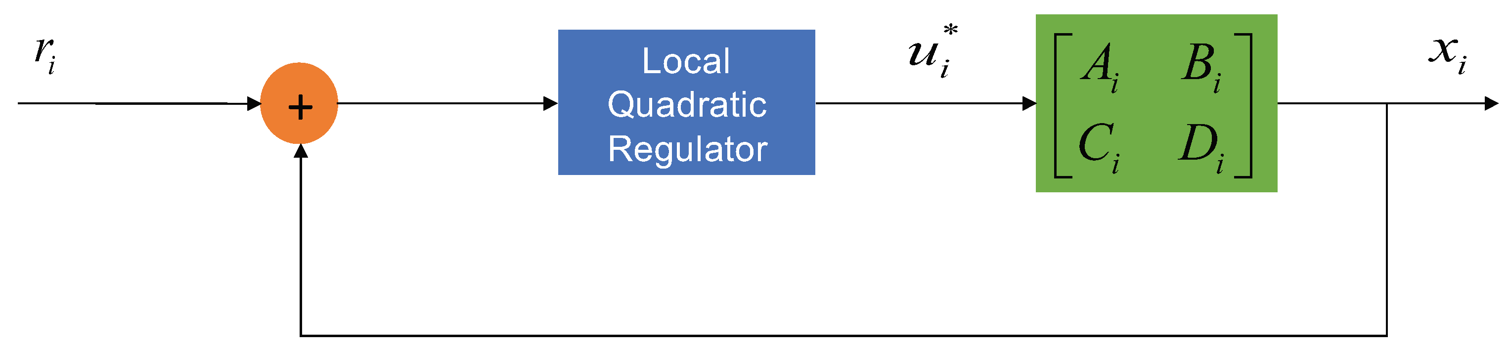
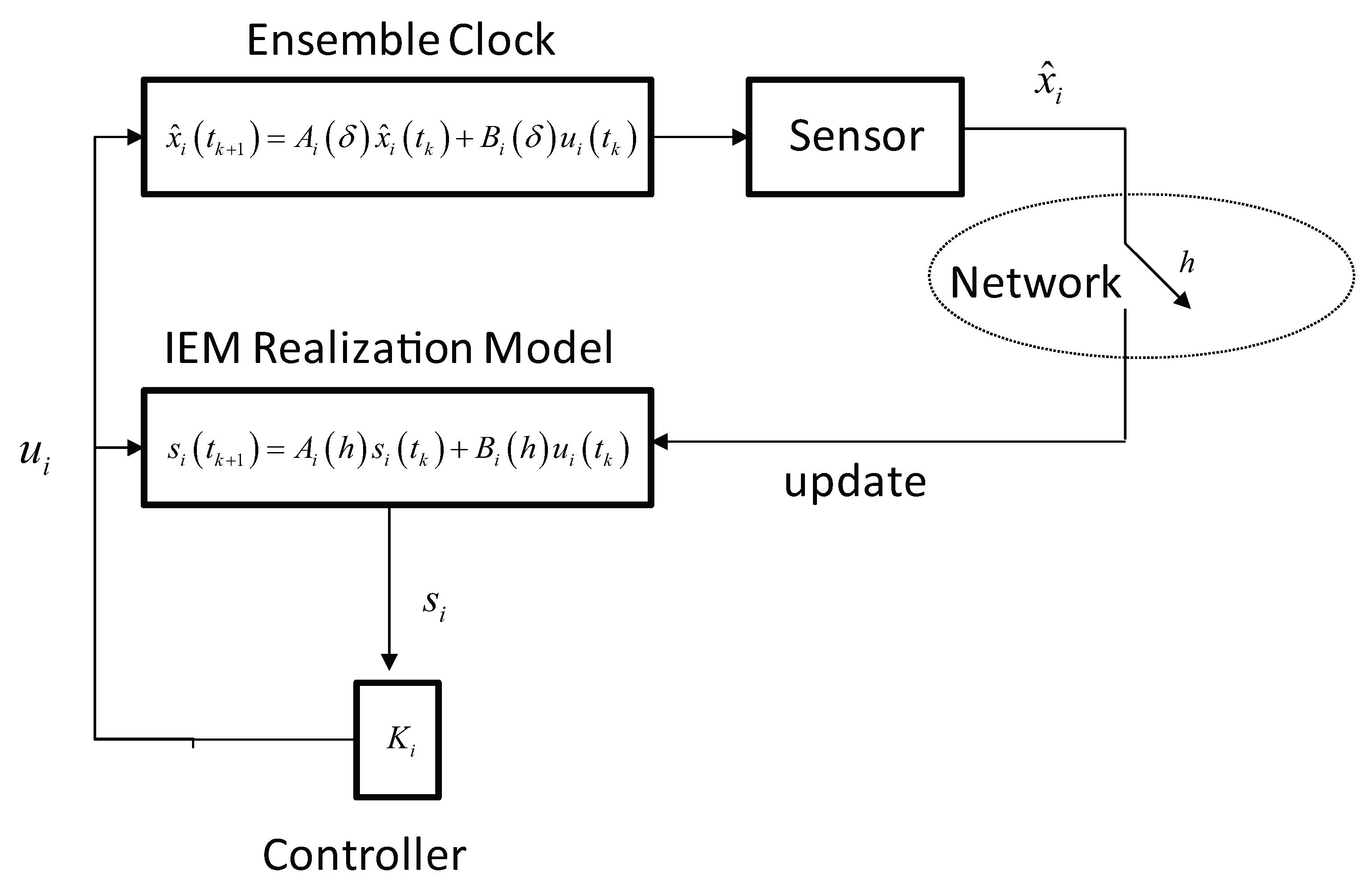
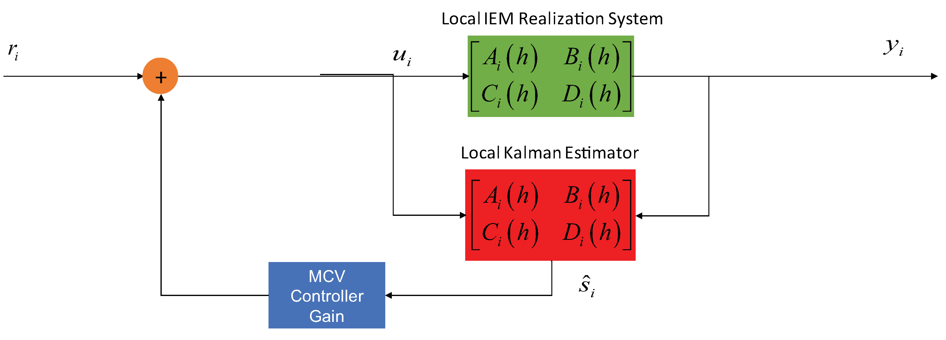
Under suitable conditions where both process and measurement noises are Gaussian, the design of stochastic control herein can be further extended and thus divided into two separate problems, one of optimal control with full state information and one of filtering. The remainder of the research investigation is to present a framework for the separation principle, which is more in line with basic engineering thinking, e.g., the optimal feedback law for steering commands is linear in the data feedback and given by

$$\begin{array}{c}\hfill u_i^{*}\left(t_k\right)=K_i\left(t_k\right){\widehat{s}}_i\left(t_k\right)\end{array}$$

(112)

where ${\widehat{s}}_i\left(t_k\right)$ is obtained by a local Kalman state estimator. Each platform i in Figure 11 uses the steering command (112) based on the Kalman state estimator for feedback frequency adjustments to ensure that the phase offset between the steerable OCXO and the IEM estimate is driven to zero.

7. Conclusions

This article highlights the promising concept of an emergent time scale in AltPNT and addresses the technical challenges of achieving onboard ensemble time scale autonomy, primarily through inter-platform measurements. While the initial findings may seem simplified, they are intended to ignite a stronger interest in developing and deploying onboard ensemble time scales within pLEO constellations.

AltPNT is vital for the success of satellite constellations, which are meant to be reconstituted every three to five years. Research shows that assembling flexible ensemble time scales across pLEO constellations is not only feasible but can be efficiently performed through on-orbit assembly. This innovative process leverages autonomous networked control of time scale realizations, both during and after integrating crucial information about IEM estimation into inter-platform communication networks. Moreover, employing existing satellite crosslinks and expertly navigating the trade-offs between open-loop and closed-loop control greatly affects the control interval, highlighting its importance in effective clock steering. This approach is not just a technical possibility; it is a transformative step forward in satellite technology, which paves the way for enhanced precision and reliability in navigation and timing.

Achieving high-precision time synchronization is essential and hinges on a comprehensive understanding of first-order Doppler effects, which influence frequency changes in received signals. These changes are directly tied to the relative position and velocity of orbital platforms. This subject stands apart from the existing literature surrounding clock ensemble generation and realization, which emphasizes its unique importance.

A resilient method is proposed for delivering precision timing across a distributed architecture, which involves discreet data transport between the anchor orbital platform and the participating platforms. This innovative approach guarantees exceptional communication performance through ad hoc, non-dedicated requests for clock data transport while optimizing power allocation to fulfill diverse service needs.

Furthermore, the autonomous assembly of active MCV controllers plays a pivotal role in precisely synchronizing one frequency standard with another. This process ensures the creation of an onboard low SWaP time scale backup, which is in phase and frequency with the IEM reference. Thanks to the robustness of the MCV control algorithm, reliable time scale realizations can be achieved even in the face of stochastic noise processes and performance uncertainties that exceed expected thresholds. This robust framework paves the way for advancing precision timing in orbital contexts, making it an investment worth pursuing.

The findings presented here underscore the significant opportunity in achieving unparalleled operational effectiveness and efficiency in ad hoc and non-dedicated pLEO services, especially under extreme radio conditions like GNSS outages. By leveraging local autonomous agents onboard pLEO constellations, one can facilitate an innovative integration of primary satellite communication and secondary PNT services at the physical layer. This integration is guided by regulatory policies, which are informed by data link layers and forecasts on link capacity resources, thus paving the way for enhanced reliability and performance.

Looking ahead, we see future work focusing on modeling, simulation, and analysis to conduct trade-off studies aimed at achieving remarkable 100-picosecond radio time synchronization across the constellation, utilizing advanced software-defined radios in collaboration with leading teams. Additionally, the development of ensemble algorithms will be explored to effectively deploy both local and remote clocks at scale. This initiative aims to ensure precise timing distribution across distant assets while addressing challenges such as clock drift, network latency, Doppler effects, and relativistic influences.

To support this experimental framework, it is essential to identify high-performance inter-platform measurement devices. The characterization of all ensemble clocks will concentrate on defining parameters for Kalman filters, which are crucial for hardware implementation to optimize computation time per iteration. Together, these efforts promise to revolutionize the capabilities of pLEO systems and enhance our preparedness for future challenges.

References

1. McDowell, J.C. The Low Earth Orbit Satellite Population and Impacts of the SpaceX Starlink Constellation. Astrophys. J. Lett. 2020, 829, L36. [Google Scholar] [CrossRef]
2. Prol, F.S.; Ferre, R.M.; Saleem, Z.; Välisuo, P.; Pinell, C.; Lohan, E.S.; Elsanhoury, M.; Elmusrati, M.; Islam, S.; Çelikbilek, K.; et al. Position, Navigation, and Timing (PNT) Through Low Earth Orbit Satellite: A Survey on Current Status, Challenges, and Opportunities. IEEE Access 2022, 10, 83971–84200. [Google Scholar] [CrossRef]
3. Reid, T.G.; Neish, A.M.; Walter, T.; Enge, P.K. Broadcast LEO Constellation for Navigation. NAVIGATION 2018, 65, 205–220. [Google Scholar] [CrossRef]
4. Coleman, M.J.; Beard, R.L. Autonomous Clock Ensemble Algorithm for GNSS Applications. NAVIGATION 2020, 67, 333–346. [Google Scholar] [CrossRef]
5. Senior, K.L.; Coleman, M.J. The Next Generation GPS Time. NAVIGATION 2017, 64, 411–426. [Google Scholar] [CrossRef]
6. Wang, Q.; Rochat, P. ONCLE (One Clock Ensemble) for Galileoś Next-Generation Robust Timing System. NAVIGATION 2022, 69, 536. [Google Scholar] [CrossRef]
7. Gunther, C. Kepler—Satellite Navigation without Clocks and Ground Station. In Proceedings of the 31st International Technical Meeting of the Satellite Division of the Institute of Navigation (ION GNSS+ 2018), Miami, FL, USA, 24–28 September 2018; pp. 849–856. [Google Scholar]
8. Michalak, G.; Glaser, S.; Neumayer, K.H.; Konig, R. Precise Orbit and Earth Parameter Determination Supported by LEO Satellites, Inter-Satelllite Links and Synchronized Clocks of a Future GNSS. Adv. Space Res. 2021, 68, 4753–4782. [Google Scholar] [CrossRef]
9. Chaudhry, A.U.; Yanikomeroglu, H. Laser Intersatellite Links in a Starlink Constellation: A Classification and Analysis. IEEE Veh. Technol. Mag. 2021, 16, 48–56. [Google Scholar] [CrossRef]
10. Heine, F.; Brzoska, A.; Gregory, M.; Hiemstra, T.; Mahn, R.; Pimentel, P.M.; Zech, H. Status on Laser Communication Activities at Tesat-Spacecom. In Proceedings of the Free-Space Laser Communications XXXV, San Francisco, CA, USA, 30 January–1 February 2023; Volume 12413, pp. 83–93. [Google Scholar]
11. Tournear, D. Future Directions: Delivering Capabilities. In Proceedings of the Small Satellite Conference, SSC20-IV-02, Virtual, 1–6 August 2020. [Google Scholar]
12. Pham, K.D. Integrated Navigation and Communications: A Conformance Framework. In Proceedings of the IEEE Aerospace Conference, Big Sky, MT, USA, 4–11 March 2023. [Google Scholar]
13. Pham, K.D. A Timescale Concept in AltPNT: A Model-based Controls of Networked System Approach. In Proceedings of the IEEE Aerospace Conference, Big Sky, MT, USA, 1–8 March 2025. [Google Scholar]
14. Allan, D. Time and Frequency (Time-Domain) Characterization Estimation, and Prediction of Precision Clocks and Oscillators. IEEE Trans. Ultrason. Ferroelectr. Freq. Control 1987, 34, 647–654. [Google Scholar] [CrossRef] [PubMed]
15. Riley, W.J. Handbook of Frequency Stability Analysis; National Institute of Standards and Technology: Gaithersburg, MD, USA, 2008.
16. Greenhall, C.A. Kalman Filter Clock Ensemble Algorithm That Admits Measurement Noise. Metrologia 2006, 43, S311. [Google Scholar] [CrossRef]
17. Senior, K.; Coleman, M.J. Generation of Ensemble Timescales for Clocks at the Naval Research Laboratory. In Proceedings of the 2014 Precise Time and Time Interval Meeting, Boston, MA, USA, 1–4 December 2014; pp. 98–105. [Google Scholar]
18. Gödel, M.; Furthner, J. Robust Ensemble Time Onboard a Satellite. In Proceedings of the 48th Annual Precise Time and Time Interval Systems and Applications Meeting, Monterey, CA, USA, 30 January–2 February 2017; pp. 26–43. [Google Scholar]
19. Tryon, P.V.; Jones, R.H. Estimation of Parameters in Models for Cesium Beam Atomic Clocks. J. Res. Natl. Bur. Stand. 1983, 88, 71–81. [Google Scholar] [CrossRef] [PubMed]
20. Malykin, G.B. The Sagnac Effect: Correct and Incorrect Explanations. Physics-Uspekhi 2000, 43, 1229. [Google Scholar] [CrossRef]
21. Shen, D.; Chen, G.; Pham, K.D.; Blasch, E. Enhanced Multi-Way Time Transfer for High-Precision Time Synchronization among UASs. In Proceedings of the IEEE Military Communications Conference, Rockville, MD, USA, 28 November–2 December 2022. [Google Scholar]
22. Stein, S.R. Time Scales Demystified. In Proceedings of the 2003 IEEE International Frequency Control Symposium and PDA Exhibition Jointly with the 17th European Frequency and Time Forum, Tampa, FL, USA, 4–8 May 2003; pp. 223–227. [Google Scholar]
23. Zucca, C.; Tavella, P. The Clock Model and Its Relationship with the Allan and Related Variances. IEEE Trans. Ultrason. Ferroelectr. Freq. Control 2005, 52, 289–296. [Google Scholar] [CrossRef] [PubMed]
24. Farina, M.; Galleani, L.; Tavella, P.; Bittanti, S. A Control Theory Approach to Clock Steering Techniques. IEEE Trans. Ultrason. Ferroelectr. Freq. Control 2010, 57, 2257–2270. [Google Scholar] [CrossRef] [PubMed]
25. Montestruque, L.A.; Antsaklis, P.J. On The Model-Based Control of Networked Systems. Automatica 2003, 39, 1837–1843. [Google Scholar] [CrossRef]
26. Pham, K.D.; Sain, M.K.; Liberty, S.R. Infinite Horizon Robustly Stable Seismic Protection of Cable-Stayed Bridges Using Cost Cumulants. In Proceedings of the American Control Conference, Boston, MA, USA, 30 June–2 July 2004; pp. 691–696. [Google Scholar]
27. Pham, K.D.; Jin, G.; Sain, M.K.; Spencer, B.F., Fr.; Liberty, S.R. Generalized LQG Techniques for the Wind Benchmark Problem. Spec. Issue ASCE J. Eng. Mech. Struct. Control Benchmark Probl. 2004, 130, 466–470. [Google Scholar]
28. Pham, K.D.; Sain, M.K.; Liberty, S.R. Cost Cumulant Control: State-Feedback, Finite-Horizon Paradigm with Applications to Seismic Protection. Spec. Issue J. Optim. Theory Appl. 2002, 115, 685–710. [Google Scholar] [CrossRef]
29. Pham, K.D. Minimal Variance Control of Clock Signals. In Proceedings of the IEEE Aerospace Conference, Big Sky, MT, USA, 5–12 March 2016; pp. 1–8. [Google Scholar]
Figure 1. pLEO time scale interoperability using existing communication infrastructures.
Information 16 00210 g001
Figure 2. Superimposing of communication and clock data signals in the proposed ICaC.
Information 16 00210 g002
Figure 3. A Discrete-Time System for the proposed ICaC.
Information 16 00210 g003
Figure 4. Local quadratic regulators for the ICaC.
Information 16 00210 g004
Figure 5. A pLEOT time scale concept for AltPNT.
Information 16 00210 g005
Figure 6. Inter-platform measurements.
Information 16 00210 g006
Figure 7. The proposed Enhanced Multi-Way Time Transfer (EM-WaTT).
Information 16 00210 g007
Figure 8. Interconnections of clock-to-clock difference measurements and Kalman filters onboard anchor platform.
Information 16 00210 g008
Figure 9. Implicit ensemble mean realizations aboard pLEO platforms.
Information 16 00210 g009
Figure 10. Local time scale realizations via networked control systems.
Information 16 00210 g010
Figure 11. Local time scale realizations via Kalman estimators.
Information 16 00210 g011
Disclaimer/Publisher’s Note: The statements, opinions and data contained in all publications are solely those of the individual author(s) and contributor(s) and not of MDPI and/or the editor(s). MDPI and/or the editor(s) disclaim responsibility for any injury to people or property resulting from any ideas, methods, instructions or products referred to in the content.