Abstract
Buildings account for approximately one-third of global energy usage and associated carbon emissions, making energy benchmarking a crucial tool for advancing decarbonization. Current benchmarking studies have often been limited to mainly the annual scale, relied heavily on simulation-based approaches, or employed regression methods that fail to capture the complexity of diverse building stock. These limitations hinder the interpretability, generalizability, and actionable value of existing models. This study introduces a hybrid AI framework for building energy benchmarking across two time scales—annual and monthly. The framework integrates supervised learning models, including white- and gray-box models, to predict annual and monthly energy consumption, combined with unsupervised learning through neural network-based Self-Organizing Maps (SOM), to classify heterogeneous building stocks. The supervised models provide interpretable and accurate predictions at both aggregated annual and fine-grained monthly levels. The model is trained using a six-year dataset from Washington, D.C., incorporating multiple building attributes and high-resolution weather data. Additionally, the generalizability and robustness have been validated via the real-world dataset from a different climate zone in Pittsburgh, PA. Followed by unsupervised learning models, the SOM clustering preserves topological relationships in high-dimensional data, enabling more nuanced classification compared to centroid-based methods. Results demonstrate that the hybrid approach significantly improves predictive accuracy compared to conventional regression methods, with the proposed model achieving over 80% at the annual scale and robust performance across seasonal monthly predictions. White-box sensitivity highlights that building type and energy use patterns are the most influential variables, while the gray-box analysis using SHAP values further reveals that Energy Star® rating, Natural Gas (%), and Electricity Use (%) are the three most influential predictors, contributing mean SHAP values of 8.69, 8.46, and 6.47, respectively. SOM results reveal that categorized buildings within the same cluster often share similar energy-use patterns—underscoring the value of data-driven classification. The proposed hybrid framework provides policymakers, building managers, and designers with a scalable, transparent, and transferable tool for identifying energy-saving opportunities, prioritizing retrofit strategies, and accelerating progress toward net-zero carbon buildings.
1. Introduction
The building sector accounts for around one-third of global energy consumption and carbon emissions, making it one of the most significant contributors to worldwide totals [1,2]. Energy efficiency interventions in building industries are essential for limiting climate change impacts and remain central to the international commitment to reach low emissions by 2050 (global Net Zero 2050 target) [3,4]. Countries including the United States, China, members of the European Union, India, Canada, Brazil, etc., have embraced energy benchmarking regulations, reporting significant advances in curbing both energy demand and greenhouse gas emissions [5,6,7]. As such, energy conservation for buildings is central to achieving international decarbonization goals. Both operational improvements in existing buildings and low-carbon strategies in new construction are urgently required to reduce demand on energy systems and mitigate climate risks. Over the past several decades, a variety of strategies have been developed, such as retrofit programs, energy efficiency codes, financial incentive schemes, and large-scale modeling of urban energy systems [8,9,10]. Among these approaches, energy benchmarking has emerged as a particularly practical and widely adopted method, enabling stakeholders to measure, compare, and track performance over time and against peer buildings [11,12,13]. Benchmarking provides standardized metrics that can guide both policy design and individual decision-making, offering a bridge between technical analysis and actionable energy savings [14].
Two broad methods of benchmarking approaches exist: simulation-based and data-driven [15]. Simulation-based benchmarking uses physics-based engines, such as EnergyPlus, eQuest, and DOE-2, to estimate energy consumption profiles from detailed inputs on building geometry, materials, climate conditions, and operational schedules [16]. Although these tools are powerful, they face well-known limitations. First, they demand highly granular data inputs that are often unavailable in practice [17]. Second, simulated results frequently diverge from measured consumption, leading to questions of reliability. Finally, models developed for a particular case or climate zone are difficult to generalize across broader contexts [18]. These challenges have prompted increased attention to data-driven benchmarking, which leverages statistical and machine learning models to analyze measured datasets. By learning directly from empirical data, such methods can be applied at scale and updated dynamically as new data becomes available [19].
In recent years, the increase in smart meters, open government data portals, and advanced AI techniques has accelerated research into data-driven benchmarking. Many studies have concentrated on annual benchmarking. For example, Park et al. [20] applied data-mining techniques to office buildings; Robinson et al. [21] analyzed more than 2600 commercial buildings under New York City’s benchmarking program named Local Law 84; Chen et al. [22] proposed a Lorenz-curve-based annual benchmark for mixed-use buildings. Similarly, Papadopoulos et al. (2017) [9] introduced a cross-city benchmark system using EUI and CO2 in the United States; and Arjunan et al. [10] highlighted the significance of building features across diverse U.S. locations by linear and ensemble learning models. More recently, Li et al. [13] advanced the field with a generalized benchmarking framework based on XGBoost, introducing post-prediction evaluation for improved interpretability. Collectively, these studies demonstrate the robustness of annual benchmarking, yet also expose its limitations: annual metrics mask seasonal fluctuations and short-term dynamics that are critical for operational management.
To address this gap, several studies have begun to focus on monthly benchmarking. Catalina et al. [23] demonstrated regression-based models for monthly heating demand in residential buildings. Vaisi et al. [24] applied a monthly benchmarking approach to secondary schools in Iran using statistical analysis, identifying influential building attributes for management strategies. Li et al. [11] proposed a hybrid approach that integrated unsupervised and supervised models, achieving superior accuracy in monthly electricity and natural gas predictions. Despite these advances, monthly benchmarking studies remain relatively rare, and most classifications focus narrowly on a small set of features such as building type or climate zone [25,26]. This narrow scope limits interpretability and fails to capture the full diversity of building stock. Moreover, the relationship between monthly and annual benchmarks remains underexplored. While annual benchmarks support cross-building comparison and long-term policy design, monthly benchmarks capture fine-grained operational patterns. Integrating the two scales promises a more holistic and actionable understanding of building energy performance.
Another important challenge is how buildings are classified for benchmarking. Conventional approaches group buildings by type (e.g., office, residential, educational) or by single attributes such as floor area or year built [27]. This oversimplification fails to reflect the heterogeneity of energy-use patterns across the stock. Unsupervised clustering methods have been applied to improve classification, with K-Means being among the most commonly used [11,28]. However, centroid-based algorithms such as K-Means and K-Means++ assume linear separability and spherical clusters, are sensitive to initialization, and often overlook nonlinear attribute interactions. In contrast, Self-Organizing Maps (SOM) provide a neural-based, topology-preserving method that converts high-dimensional input data onto a low-dimensional grid, preserving neighborhood relations [29,30]. SOM has been applied in diverse fields successfully, like pattern recognition, image analysis, and environmental modeling, and its ability to reveal nonlinear and latent structures makes it highly suitable for building energy classification. Yet its potential in energy benchmarking remains underutilized.
Table 1 illustrates the location, contribution, and research gaps discussed from existing studies. In this study, the authors propose a hybrid AI-driven framework that integrates the state-of-the-art supervised prediction with SOM-based clustering models to benchmark building energy use across two time scales: annual and monthly. The framework combines the strengths of white- and gray-box models—Multiple Linear Regression (MLR) for interpretability and Light Gradient Boosting Machine (LGBM) for predictive accuracy. Using a comprehensive six-year dataset from Washington, D.C., including significant building attributes, energy consumption, and weather variables, the study demonstrates how SOM can uncover nuanced building categories and how supervised learning models can leverage these classifications for robust prediction. Additionally, this study investigates the energy use patterns across two important time scales for policymakers and building managers. The specific objectives of this research are as follows:

Table 1.
The location, model, contribution, and research gap from the existing studies (sorted by published year).
- Develop a hybrid supervised and unsupervised learning framework for energy benchmarking across two time scales, integrating both annual and monthly perspectives.
- Provide interpretability and sensitivity analyses of building attributes across scales, highlighting the impacts/roles of building attributes and climate factors.
- Demonstrate the advantages of SOM in classifying heterogeneous building stocks to challenge traditional building classifications.
- Offer a replicable and transferable framework for cities and regions seeking scalable energy benchmarking methods to support decarbonization.
2. High-Granularity Dataset and Methodology
This study develops a hybrid AI framework that integrates supervised plus unsupervised models to benchmark building energy consumption across two time scales: annual and monthly. The framework is designed to (i) benchmark and predict energy performance with a balance between interpretability and predictive accuracy, and (ii) classify heterogeneous building stocks in a data-driven and unbiased manner. The methodology consists of four main stages: data acquisition and preprocessing, supervised prediction with linear (MLR) and tree-based ensemble learning models, including Random Forest (RF) and LGBM, unsupervised clustering using SOM, and interpretability analysis of key building attributes. MLR model is widely used in industry; therefore, it is set as the baseline model in this study. The workflow of this study can be illustrated in Figure 1.
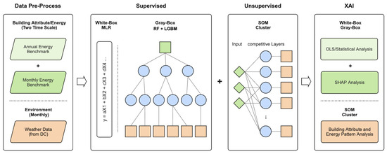
Figure 1.
Hybrid data-driven building energy benchmarking analysis across two time scales workflow.
2.1. Data Collection and Preprocessing
The primary dataset is obtained from the Washington, D.C. Open Data portal, which provides annual and monthly benchmarking records of commercial and institutional buildings. The benchmarking dataset information can be found: https://opendata.dc.gov/datasets/DCGIS::building-energy-benchmarking/about, accessed on 16 May 2025. To enrich the dataset and account for climatic influences, we incorporate high-frequency weather data (temperature, humidity, solar radiation, and wind speed) from the National Renewable Energy Laboratory (NREL) [31]. The weather data and descriptions can be found: https://nsrdb.nrel.gov/data-viewer, accessed on 16 May 2025. The raw dataset includes more than 10,000 records across six years from 2018 to 2023, spanning diverse building types, Energy Star® ratings, operational profiles, and climatic conditions.
Data preprocessing is conducted in several steps. First, categorical attributes such as building type are transformed into a numerical format through one-hot encoding (OHE), ensuring compatibility with machine learning models. Second, continuous features, including energy use intensities (EUIs), are examined for skewness and normalized using a generalized logarithmic (GLOG) transformation, following [32]. Third, outlier detection is performed using a z-score based approach, removing approximately 8% of anomalous values in energy, construction year, and weather attributes, consistent with prior data-cleaning protocols in energy studies [33]. After cleaning, the dataset contains 9609 usable cases and 109 variables, forming a robust basis for subsequent analysis. The electricity and natural gas usage distributions among all 12 months are shown in Figure 2.
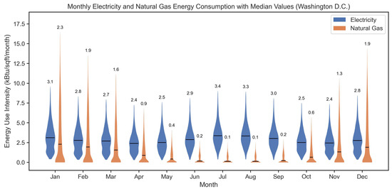
Figure 2.
Electricity and natural gas energy consumption distributions among all 12 months in Washington D.C. from 2018 to 2023.
2.2. Supervised Prediction Models
For the first stage, the supervised regression-based models are trained to predict energy consumption at both annual and monthly scales. We have adopted two model categories: (i) MLR, representing a white-box approach and set it as a baseline model [34], and the well-known Energy Star® rating system from the building industry also employs MLR models; (ii) RF + LGBM, representing the gray-box ensemble method [35,36]. The training and test datasets are split into 70% and 30%.
MLR provides interpretable coefficients that directly quantify the relationship between building attributes and energy consumption, providing a more straightforward approach for understanding the relationship between input variables and predictive energy usage compared to the other non-linear models [37,38]. Although linearity assumptions may limit predictive accuracy, MLR serves as a transparent benchmark, allowing clear attribution of variance to individual factors. The objective function for MLR in this study can be expressed as Equation (1).
where y denotes the predictive energy usage values, the intercept, the slope coefficients for each building attribute variable, the predictor variables, and c a constant offset.
Ensemble learning models integrate multiple base learners to enhance predictive accuracy. They are generally categorized into independent and dependent ensembles [39]. Independent ensembles, such as Bagging and RF, train multiple models in parallel on resampled subsets of data and aggregate their predictions to reduce variance [39]. In contrast, dependent ensembles, such as Boosting (e.g., LGBM, XGBoost), build models in order, where each new learner reduces the errors from the previous iterations [11].
To compare the predictive performance of the baseline white-box MLR model, this study employs both RF and LGBM as representatives of independent and dependent ensemble learning models. RF independently constructs multiple decision trees using bootstrapped samples and random feature selection, and aggregates their outputs through averaging [28,39]. RF is an advanced ensemble learning model and has been utilized in several benchmarking studies [26,36].
LGBM is a dependent ensemble learning model that constructs gradient-boosted decision trees with high efficiency and predictive power [35]. Compared to other tree-based methods, such as RF and XGBoost, LGBM is computationally more efficient and less prone to overfitting when properly regularized. As such, it is selected as the representative for the gray-box model category [11]. In this study, hyperparameters are optimized through grid search with cross-validation, using mean squared error (MSE) as the primary loss function. The comparison between LGBM and RF thus provides a balanced evaluation between dependent (boosting-based) and independent (bagging-based) ensemble approaches, highlighting the robustness and efficiency of the proposed model relative to other widely used state-of-the-art benchmarks. Equation (2) is the objective function of the LGBM model with MSE as the evaluation metric.
where N is the number of training building samples, denotes the true target value (or one-hot encoded vector) of the building, and represents its predicted value. The first term measures the mean MSE between predicted and actual targets, ensuring model accuracy. The second and third terms correspond to (Lasso) and (Ridge) regularization, controlled by coefficients and , respectively, to prevent overfitting and enhance generalization. The final term penalizes model complexity by constraining the number of leaf nodes T in the decision trees, encouraging compact, interpretable models. This formulation reflects the trade-off between model fit, sparsity, and complexity—core to the LGBM framework’s efficiency and robustness.
2.3. Model Evaluation and Interpretability
Model performance is assessed through two essential metrics: the coefficient of determination () to evaluate variance explained [40], and root mean squared error (RMSE) to assess predictive errors. Despite multiple evaluation metrics existing, like MSE, mean squared logarithmic error (MSLE), mean absolute error (MAE), etc., RMSE maintains the same unit as the predictive values. Therefore, RMSE is selected as the main metric in the study [41]. Evaluations are conducted separately for annual energy benchmarking and monthly predictions to capture scale-dependent differences.
Beyond predictive accuracy, XAI has emerged as a critical paradigm for improving the transparency and trustworthiness of machine learning models in building performance analysis [42]. Unlike traditional “black-box” approaches, XAI enables users to understand how input features influence model outputs, thereby bridging the gap between predictive accuracy and interpretability [12]. XAI techniques can be broadly categorized into three groups: (i) ante-hoc methods, which incorporate interpretability directly into model design, such as decision trees or linear regression; (ii) in-hoc methods, which enhance interpretability within the learning process, often through architecture constraints or attention mechanisms; and (iii) post-hoc methods, which generate explanations after model training using techniques such as Shapley Additive Explanations (SHAP) and feature importance ranking [43,44].
In this study, the degree of XAI is evaluated along a gradient of interpretability. A high degree of XAI indicates that a study not only identifies feature correlations but also offers practical approaches for interpreting or applying benchmarking results in real-world decision-making, or provides a detailed visualization of energy use patterns [38]. It also helps position the proposed model within the broader XAI framework, emphasizing both explainability and actionable insights for building stakeholders [10].
To interpret model outputs, we apply sensitivity analyses and feature importance methods. For MLR, Ordinary Least Squares (OLS) standardized coefficients are used to assess the direction and magnitude of influence. P-values, standard deviation (std) errors, t-statistics (t-tests), and 97.5% confidence intervals (CI) for each input feature are also reported to illustrate the correlations. The OLS regression is well-suited for MLR interpretation because it provides direct, transparent estimates of how each predictor linearly influences the target variable [45]. The magnitude and sign of each coefficient offer intuitive insights into variable importance and directionality, while associated p-values and confidence intervals quantify statistical significance and reliability. The OLS regression model for predicting site EUI is formulated as follows:
where represents the predicted site energy use intensity (kBtu/ft2/year) for building i, is the intercept term, denotes the estimated regression coefficient for predictor variable , and is the random error term assumed to be normally distributed with mean zero and constant variance. All categorical building types are encoded as dummy variables, and continuous predictors such as fuel use percentage, Energy Star® rating, and climatic indicators are included in their standardized form.
Although LGBM inherently provides some degree of model transparency through feature importance and decision path inspection, it remains a complex ensemble of hundreds of boosted trees, which obscures its local interpretability [46]. To achieve consistent and comparable insights across both temporal scales and models, post hoc explainability methods are therefore employed. Specifically, SHAP analysis is used to quantify each feature’s contribution to individual predictions, offering a unified interpretive framework across annual and monthly models [47]. This complementary approach ensures that explainability is not limited to global feature ranking but extended to local, sample-level reasoning, thereby enhancing transparency, robustness, and trust in the model’s decision process.
For LGBM, feature importance is derived from split gains and validated using SHAP values, which provide local and global interpretability [47]. SHAP is an advanced explainable AI (XAI) technique that attributes the contribution of each feature to individual predictive value via cooperative game theory. It provides consistent and locally accurate explanations by decomposing model outputs into additive feature effects [47,48]. For the LGBM model in this study, SHAP is particularly advantageous because it translates complex, nonlinear feature interactions into interpretable importance scores, enabling a transparent understanding of how building characteristics and climatic variables influence predicted EUIs [49]. Together, these techniques ensure that the hybrid framework not only achieves predictive accuracy but also yields actionable insights for design and policy.
Additionally, to validate the model’s generalizability, this study conducts sensitivity and robustness validation using monthly building energy benchmarking data from the City of Pittsburgh, Pennsylvania, located in ASHRAE Climate Zone 5A with a cool climate, which differs from Washington, D.C. (Climate Zone 4A). The corresponding weather data for Pittsburgh were also obtained from the NREL to ensure consistency and accuracy in climatic representation [31].
2.4. Cluster Benchmarking via SOM Unsupervised Learning
Traditional benchmarking studies often categorize buildings using type-based or centroid-based clustering methods (e.g., K-Means) [25,28,50]. While effective in certain contexts, such methods assume spherical clusters and do not preserve topological relationships among attributes. To overcome these limitations and further investigate the energy consumption patterns for each building classification after the first supervised learning predictions, we employ SOM, a neural-based unsupervised learning method originally introduced by Kohonen [29]. SOM projects high-dimensional input vectors onto a two-dimensional lattice of neurons, preserving the neighborhood relationships of the input space through competitive learning [51]. This topology-preserving property enables SOM to reveal nonlinear structures and provide more nuanced classifications compared to centroid-based methods.
In this study, SOM is applied to the preprocessed dataset to uncover latent building categories through a comprehensive set of attributes, such as building type, size, Energy Star® rating, operational characteristics, and climate variables. The SOM algorithm minimizes quantization error (QE) between input vectors and their best-matching units (BMUs), while also maintaining topological continuity measured by topographic error (TE). To assess the stability and interpretability of the resulting clusters, the study employs both Calinski-Harabasz and Silhouette score analysis [52]. Calinski-Harabasz is able to select the optimal cluster number for the SOM model, while the Silhouette score enables the identification of meaningful groups of buildings that share similar energy-use patterns but may differ from traditional type-based classifications [52,53]. The SOM objective function in this study can be expressed as Equation (4) [54]:
where N is the selected building cases (entire building stock in this study), M is the map unit numbers. Kernel is the neighborhood centered at the unit b, the optimal vector unit , and .
3. Results
The outcomes of the hybrid framework across two major components are presented: (i) Supervised prediction of EUI at annual and monthly scales using MLR, RF, and LGBM, and (ii) Unsupervised clustering using SOM to identify the optimal cluster number with classification of buildings and characteristics of each cluster. Performance is evaluated with both accuracy and interpretability metrics, followed by sensitivity analyses of influential variables.
3.1. Supervised Prediction at the Annual and Monthly Scale
The initial supervised models are trained to predict annual site EUI. Figure 3 compares observed against predicted outcomes for baseline MLR (white-box) RF, and LGBM (gray-box). Additionally, Table 2 directly shows the three model performances and computing times. In Figure 3, the X-axis is the actual value, while the Y-axis is the predicted value. The blue dots in the two sub-plots from Figure 3 illustrate good predictive performance, meaning the errors are within 15% acceptance interval thresholds. The acceptance interval threshold for the building energy prediction approach was proposed by Li et al. [13] (2024) and has proven to be a reliable method for evaluating model performance. In this study, the threshold is set as 15% accordingly.
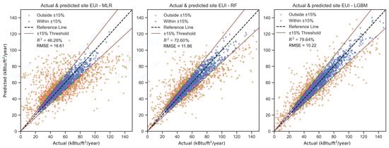
Figure 3.
Building Annual Energy Predictions for baseline Energy Star® MLR (left), RF (middle), and LGBM (right) models. The brown lines in the plots are acceptance interval thresholds of 15% prediction errors.
Table 2.
MLR, RF, and LGBM Model performance and computing time comparisons.
The baseline MLR model exhibits limited predictive capability, achieving an of approximately 0.46 and an RMSE exceeding 16.6 kBtu/ft2/year. This moderate accuracy reflects the inherent limitations of linear models in capturing complex, nonlinear relationships among building attributes. Nonetheless, the MLR model offers valuable interpretability.
In contrast, RF and LGBM models demonstrate substantially improved performance. For RF, it achieves an of 72.60% with RMSE value of 11.86. Moreover, the LGBM model performs even better than RF, attaining an close to 0.80 and a lower RMSE of 10.22 kBtu/ft2/year. The residuals are symmetrically distributed around zero, indicating minimal systematic bias across the prediction range. Computationally, LGBM is much efficient than RF (Table 2). These results underscore the advantages of tree-based ensemble learning, especially the independent ensemble learning model like LGBM, in modeling nonlinear feature interactions and heterogeneous data distributions, while maintaining interpretability through post-hoc SHAP explainability methods. Overall, the comparison highlights the trade-off between model transparency and predictive accuracy, with ensemble approaches offering a robust balance of both for large-scale building energy benchmarking.
As the LGBM model exhibits substantially higher accuracy and robustness than the RF and MLR models, it is subsequently adopted for the monthly benchmarking analysis. In this phase, separate models are trained for each month to capture temporal variability and season-dependent building energy dynamics. This approach enables examination of how predictive performance fluctuates throughout the year, reflecting the influence of climatic conditions, occupancy patterns, and HVAC system operation on model accuracy.
As summarized in Table 3, the model performance varies notably across months. The ranges from 0.46 to 0.86, while the RMSE values span from 0.88 to 3.57 kBtu/ft2/year. The highest values are achieved during February (0.86), November (0.80), and December (0.81), corresponding to colder months when building energy use patterns tend to be more consistent and predictable due to heating-dominated loads. In contrast, performance declined during the spring and early summer months (April–June), where dropped below 0.65 and RMSE values are relatively higher, suggesting greater variability in transitional-season energy consumption.
Table 3.
LGBM performance comparisons among 12 months with Pittsburgh, PA (climate zone 5A) energy benchmarking data validation for the model robustness and sensitivity ( and RMSE).
The lower values observed in months such as May (0.46) and October (0.54) indicate that fluctuating weather conditions and intermittent HVAC usage during these periods introduce nonlinearities that are more challenging to capture accurately. Nevertheless, the model maintained satisfactory prediction reliability overall, with an average of approximately 0.69 and RMSE consistently below 3.6 kBtu/ft2/year across all months. The smooth performance during mid-summer (July–August, s of 0.65 to 0.66, while RMSEs are around 1.0) highlights the model’s ability to generalize across high-load cooling seasons. These findings collectively demonstrate that while model accuracy is seasonally sensitive, the LGBM framework effectively accommodates temporal dynamics, offering a robust and scalable solution for fine-grained, month-level building energy benchmarking.
As discussed in the Methodology section, to examine the model’s generalizability and robustness beyond a single climatic context, we conducted an additional validation using monthly real-world data from Pittsburgh (Pit), PA, which is located in climate zone 5A of the United States. This dataset contains 506 building samples after preprocessing and is integrated with the Washington, D.C. dataset to evaluate model transferability across regions. The comparison results in Table 3 show that the LGBM model maintains comparable performance when applied to a different climate zone, with values consistently above 0.6–0.8 and relative low RMSE variation across months.
Additionally, integrating data from a new city can further enhance model performance, likely due to the increased diversity and number of training samples, which help the model capture broader building energy use patterns. These outcomes demonstrate that the model captures generalizable relationships rather than overfitting to a single city’s climatic conditions, thereby validating its robustness and sensitivity across multiple contexts.
The results confirm that annual benchmarking captures broad energy-use trends, while monthly benchmarking reveals scale-dependent sensitivities and operational dynamics. Importantly, the LGBM supervised framework maintained reliable performance across both scales, demonstrating its flexibility and scalability.
3.2. Sensitivity and Feature Importance
To interpret the models, feature sensitivity analyses are performed. Table 4 presents the top 25 variables ranked by their absolute OLS regression coefficients, along with standard errors, t-tests, p-values, and 97.5% confidence intervals. The regression results indicate that both building functional type and energy source composition are dominant predictors of site EUIs. Among categorical variables, Warehouse/Storage, Other Building Types, Technology/Science, and Religious Worship facilities exhibit the largest negative coefficients (ranging from to ), suggesting that these building types tend to have significantly lower EUI compared to the baseline category. These effects are statistically significant at the 95% confidence level (p < 0.05), highlighting the strong influence of occupancy type on operational energy performance.
Table 4.
OLS regression coefficients ranked by absolute coefficient (top 25) with standard errors, t-stats, p-values, and 97.5% confidence interval (CI).
The Natural Gas (%) variable shows the largest positive coefficient (, p < 0.001), indicating that buildings with a higher proportion of natural gas use generally have increased total EUI. In contrast, Electricity Use (%) is significantly negatively associated with EUI (, p < 0.001), suggesting that electrically dominated buildings—often characterized by more efficient systems—tend to consume less site energy. The Energy Star® rating also shows a strong negative coefficient (, p < 0.001), reaffirming its role as a key indicator of high energy efficiency.
Climatic factors, including June Relative Humidity (, p < 0.001), May Relative Humidity (, p < 0.001), and May DHI (Diffuse Horizontal Irradiance) (, p < 0.001), are statistically significant and reflect that humidity and solar radiation conditions contribute to variations in monthly energy demand. Several other building-type categories, such as Utility, Banking/Financial Services, and Parking, display relatively large coefficients but are not statistically significant (p > 0.1), indicating greater uncertainty in their estimated effects. Overall, the OLS regression confirms that building typology and energy supply composition are the most influential factors shaping EUI, while weather-related variables introduce seasonal variability. Although the model provides interpretability and clarity, its linear structure limits the ability to capture nonlinear interactions—motivating the adoption of the LGBM model for more accurate and robust energy benchmarking.
Figure 4 illustrates the SHAP sensitivity values for the top 15 predictive features across monthly LGBM benchmarking models. The heatmap highlights how the contribution of each variable to site EUI prediction varies throughout the year, revealing distinct seasonal and feature-level dynamics. Overall, Energy Star® Score, Natural Gas (%), and Electricity Use (%) consistently rank as the three most influential predictors, with mean SHAP values of 8.69, 8.46, and 6.47, respectively. These features collectively capture the fundamental energy performance characteristics of buildings—efficiency rating and fuel source composition—thus driving the model’s predictive accuracy across all months.
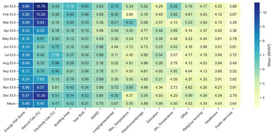
Figure 4.
LGBM model SHAP sensitivity value comparisons among the top 15 features (The heatmap columns are ranked by mean SHAP values from left to right).
Building Area and Year Built also exhibit moderate and stable influence (mean SHAP is approximately 6.4–6.2), suggesting that physical scale and construction era remain steady determinants of annual and monthly energy behavior. Climate-related and occupancy features, such as March Temperature, January Temperature, and Lodging/Residential, display seasonal fluctuations, with higher SHAP values observed during colder months (e.g., January and February) when heating loads dominate. In contrast, variables like Warehouse/Storage, Education, and Office show smaller yet consistent effects (), reflecting their more homogeneous operational profiles.
Across the year, the monthly SHAP profiles indicate that model sensitivity to climatic variables rises during transition periods (spring and fall), while energy source and efficiency indicators maintain dominant influence regardless of season. This consistent pattern confirms that LGBM effectively captures both global and local feature importance, providing interpretable insights into how building attributes and climate jointly shape energy use patterns on a month-by-month basis.
Figure 5 compares the SHAP sensitivity distributions of the top 15 influential features between a representative heating month (January) and cooling month (August). Each subplot shows the magnitude and direction of feature impacts on the predicted site EUI, where positive SHAP values indicate higher energy use and negative values reflect reductions. Clear seasonal differences are observed across the major predictors.
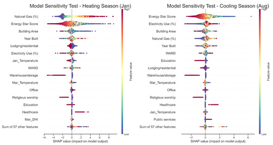
Figure 5.
LGBM model SHAP sensitivity value comparisons between heating and cooling seasons (each sub-figure is ranked by the sensitivity of the top 15 features; (left) sub-figure is from January, while (right) one is from August).
During the heating season (left panel), Natural Gas (%) and Energy Star® Score are the two most sensitive features. Buildings with a higher proportion of natural gas use show strong positive SHAP values, signifying increased heating energy demand, while higher Energy Star® scores correspond to negative SHAP values, indicating lower EUI for more efficient buildings. Building Area and Year Built also have moderate effects. Climate-related features such as January Temperature show negative gradients, as warmer outdoor conditions reduce heating requirements. Occupancy-related variables, such as Lodging/residential and Warehouse/storage, display negative effects, depending on operational intensity and hours of use.
In the cooling season (right panel), model sensitivity shifts toward Energy Star® Score and Electricity Use (%), reflecting the dominance of cooling-related energy consumption. Higher Electricity Use (%) contributes positively to EUI, capturing increased electricity demand for air-conditioning. In contrast, Natural Gas (%) becomes less influential, with more balanced SHAP distributions. Building Area, Year Built, and Education remain moderately important, while the influence of temperature variables (March Temperature and January Temperature) reverses, as higher temperatures now correspond to higher cooling energy use.
Overall, the comparison between heating and cooling seasons shows that fuel type, efficiency rating, and climatic factors have strong direction-dependent impacts on EUI predictions. The LGBM model, interpreted through SHAP values, effectively captures these nonlinear and seasonal variations, providing a transparent understanding of how building characteristics and weather jointly affect heating and cooling energy performance.
3.3. Unsupervised Clustering with SOM
The SOM model is trained on the full preprocessed combined dataset to uncover latent structures in building energy-use patterns. A two-dimensional hexagonal lattice of neurons is used, providing a balance between resolution and interpretability. Training is iterated until QE stabilized, while TE remained a relatively low value, indicating that the mapping preserved neighborhood relationships reliably. The trained grid size for SOM is 13 × 13, the learning rate is 0.25, the neighborhood function is a Gaussian distribution, and the number of iterations is 80,000, with a random seed of 200.
Figure 6 presents the Calinski-Harabasz (CH) score used to evaluate the optimal number of clusters for the SOM after supervised learning. The CH index measures cluster separation and compactness, where higher scores indicate better-defined and more distinct clusters. The results show that the CH score increases steadily from two to five clusters and reaches its peak at six clusters (137.8), followed by a gradual decline beyond seven clusters. This pattern suggests that partitioning the dataset into six clusters achieves the best balance between intra-cluster size and separation, indicating a well-structured clustering configuration for the subsequent analysis of building characteristics and energy use patterns.
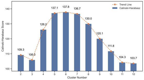
Figure 6.
Som Calinski Harabasz Score for each cluster number.
Figure 7 illustrates the Silhouette score distributions for SOM clustering models ranging from three to eight clusters. The Silhouette coefficient quantifies the degree of similarity within clusters relative to other clusters, where higher mean values reflect more coherent grouping. The average scores increase from 0.13 at K = 3 to a maximum of 0.29 at K = 6, before slightly decreasing at K = 8. The cluster shapes at K = 6 show distinct and well-separated boundaries with balanced sample sizes across clusters, confirming the clustering stability identified by the Calinski-Harabasz index. Therefore, six clusters are selected as the optimal SOM configuration for this study to characterize diverse building groups and their corresponding energy use patterns.
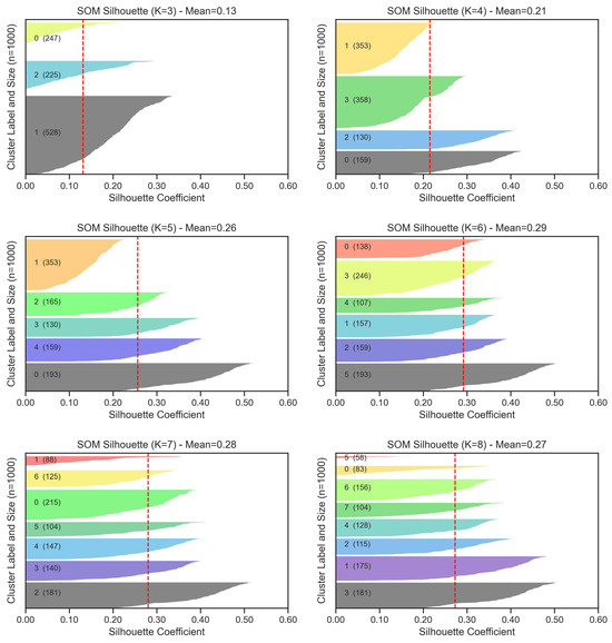
Figure 7.
SOM Silhouette score comparisons for each cluster number.
Figure 8 illustrates the distributions of building year and building area across all six SOM clusters, highlighting distinct physical characteristics within each group. The left violin plot shows that most clusters are composed of relatively modern buildings constructed after 1975, though Clusters 1 and 3 stand out with a wider range extending back to the early 1900s, indicating a mix of older and newer structures. Clusters 0, 2, 4, and 5 have median construction years around 1990–2000, suggesting that these clusters represent more contemporary building stocks.
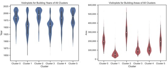
Figure 8.
Violinplots for building area and built year of all 6 clusters (from Cluster 0 to 5).
The right violin plot from Figure 8 presents the distribution of building floor areas, revealing considerable variation among clusters. Cluster 2 contains the largest buildings on average, with several exceeding 400,000 square feet, while Clusters 1, 3, and 4 primarily consist of smaller buildings below 150,000 square feet. Cluster 0 and Cluster 5 show intermediate building sizes with moderate dispersion. Together, these patterns indicate that the six clusters capture diverse combinations of age and scale—ranging from older, smaller buildings to large, recently constructed facilities—providing a meaningful basis for analyzing how building characteristics relate to distinct energy use patterns.
Figure 9 illustrates the distribution of building types across the six SOM clusters, revealing distinct and heterogeneous compositions for each group. None of the clusters exhibits similar type distributions, indicating that the SOM algorithm captures deeper structural and operational patterns beyond traditional building-use categories. Clusters 0 and 2 are dominated by mixed-use and other commercial types, whereas Cluster 1 contains a more balanced mix of lodging/residential, warehouse/storage, and service-oriented buildings. Cluster 3 features a high proportion of education and lodging/residential buildings, while Cluster 4 combines lodging/residential and office buildings with smaller shares of mixed-use and public services. Cluster 5, in contrast, is primarily composed of banking/financial services, lodging/residential, and healthcare buildings, suggesting a different group pattern compared to others.
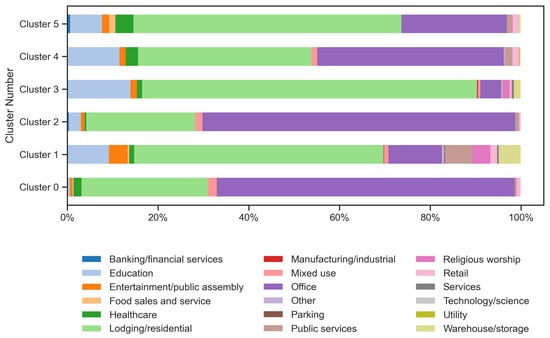
Figure 9.
Building type distributions for all 6 clusters (from Cluster 0 to 5).
These diverse type distributions highlight that the SOM-based clustering approach challenges conventional building classification systems, which often rely solely on building type as the main grouping criterion. By integrating multiple physical, operational, and environmental attributes—including floor area, construction year, fuel usage percentile, and climatic conditions—the SOM framework identifies clusters that reflect true multi-dimensional energy behavior rather than simplistic categorical distinctions. This comprehensive, data-driven approach minimizes bias associated with single-variable classification and provides a more objective foundation for analyzing building energy performance across complex building portfolios.
Figure 10 presents the monthly EUI distributions for the six SOM clusters during the heating season (November to February) and the cooling season (June to September). The results reveal clear distinctions regarding energy use patterns in clusters, while buildings within the same cluster display relatively consistent monthly EUI levels. This consistency validates the SOM clustering process, indicating that each cluster effectively groups buildings with similar seasonal energy behaviors.
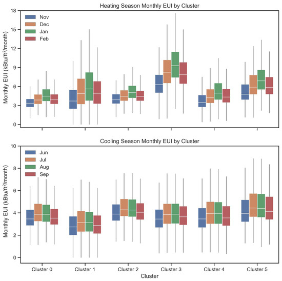
Figure 10.
Building monthly energy use pattern distributions for heating (from November to February) and cooling (from June to September) seasons of all 6 clusters (from Cluster 0 to 5).
During the heating season (top panel), significant variations are observed among clusters. Clusters 1 and 3 show the highest median EUIs, suggesting that greater heating energy demand is likely associated with larger or older building stocks. In contrast, Clusters 0 and 2 demonstrate lower and more stable EUIs, reflecting either newer construction or improved envelope and system efficiencies. Clusters 4 and 5 maintain moderate energy use with narrower distributions, implying more consistent heating operation and better energy management practices within these groups.
For the cooling season (bottom panel), the inter-cluster differences persist but at a lower magnitude. Clusters 2 and 5 exhibit higher EUIs, indicating greater cooling requirements, while Clusters 1 and 3 show more compact distributions and lower energy use levels. Across all clusters, intra-cluster patterns remain stable between June and September, confirming seasonal coherence in energy consumption behavior.
Overall, the monthly EUI analysis demonstrates that the six SOM-derived clusters capture meaningful differences in both heating and cooling energy use patterns. While traditional classifications by building type often overlook such variability, the SOM-based clustering identifies groups of buildings that share consistent, data-driven operational characteristics—enhancing interpretability and providing a robust foundation for targeted energy benchmarking and management strategies. The characteristics summary of each cluster is shown in Table 5.
Table 5.
Cluster characteristics summary table (dominant type, median built year, median building area, mean EUIs of heating and cooling seasons).
While the SOM model identified six optimal clusters based on the Calinski-Harabasz and Silhouette scores, their significance extends beyond numerical optimization. Each cluster represents a distinct operational archetype of buildings characterized by specific combinations of typology, scale, and energy-use behavior. Clusters 1 and 3 are dominated by older and smaller facilities with higher heating loads, whereas Clusters 0 and 2 comprise newer or larger mixed-use buildings exhibiting lower and more stable EUIs. Clusters 4 and 5 include residential and service-oriented buildings with moderate energy intensity and consistent year-round operation. These differences suggest that the SOM-based clusters capture nuanced variations in energy performance that conventional type-based groupings overlook. Practically, such clusters can guide targeted policy interventions and can serve as benchmarks for peer-to-peer comparison within each group. For example, prioritizing envelope retrofits for high-intensity clusters or tailoring incentive programs for efficient ones. By translating data-driven clusters into interpretable building categories, the SOM framework enhances both the analytical depth and practical applicability of energy benchmarking.
4. Discussion
The findings of this study highlight the methodological and practical significance of integrating supervised learning (e.g., MLR, RF, and LGBM) with unsupervised learning models (e.g., SOM) for building energy benchmarking at two time scales. This section consolidates the implications into three main themes: (i) dual-time scale across annual and monthly benchmarking and the balance between interpretability and accuracy, (ii) SOM-based classification and its advantages over conventional building classification approaches, and (iii) practical relevance, limitations, and future opportunities.
4.1. Dual-Scale Insights and the Balance Between Accuracy and Interpretability
One major contribution of this research is the integration of both annual and monthly scales into a unified benchmarking framework. Annual benchmarking provides stability for cross-building comparisons, capturing long-term trends and enabling policy-level evaluations [42]. However, it tends to obscure seasonal fluctuations. Monthly benchmarking, by contrast, captures operational dynamics and seasonal variations that are highly relevant to facility managers [11,55].
The results demonstrate the value of combining these two perspectives. For example, December and June yielded strong predictive accuracy, reflecting consistent heating and cooling demands, whereas transitional months such as April and September displayed weaker performance due to variability in occupant behavior and fuel switching. This dual-scale perspective offers a richer understanding of building performance and provides actionable intelligence at both strategic and operational levels.
The hybrid supervised models further enhanced this dual-scale framework. The white-box MLR model (widely used in the building industry, like Energy Star® rating system), although less accurate, delivered transparency that is essential for policy and compliance contexts. The grey-box LGBM significantly outperformed MLR in predictive accuracy, and with the addition of SHAP interpretability methods, its outputs could be decomposed into understandable drivers of energy use. Together with SOM classification, these supervised models form a multi-layered toolkit that balances accuracy with interpretability. This balance is critical in practice, as stakeholders range from policymakers seeking clarity to practitioners requiring precision.
4.2. SOM-Based Classification and Benchmarking Implications
A key methodological advance of this study is the application of SOM for unsupervised clustering. Conventional benchmarking practices often classify buildings by type, floor area, or a limited number of attributes, oversimplifying the complexity of energy-use patterns [25,28,56,57]. Centroid-based clustering algorithms, such as K-Means, partially address this issue but are constrained by assumptions of spherical clusters and sensitivity to initialization. In contrast, SOM preserves topological continuity in the high-dimensional feature space, enabling more nuanced and interpretable representations of building categories.
The clusters derived from SOM reveal patterns that would be overlooked by traditional classifications. For instance, certain educational buildings are grouped with small residential facilities due to similar energy-use dynamics, while office buildings are separated into distinct subcategories based on floor area and electricity dependence. These results illustrate the heterogeneity of building energy behavior and demonstrate the inadequacy of conventional typology-based grouping. By revealing hidden relationships, SOM enables a more equitable and scientifically robust approach to benchmarking, one that is better suited for informing data-driven energy policies and management strategies.
4.3. Practical Relevance, Limitations, and Future Directions
The hybrid framework has significant implications for building owners, policymakers, and designers. Facility managers can use cluster-informed predictions to prioritize retrofits and operational changes. For instance, older, gas-reliant buildings are shown to be highly sensitive to heating loads, suggesting that insulation upgrades and heating system improvements would yield large benefits. Policymakers can leverage SOM-based categories to design benchmarking programs that more accurately reflect the diversity of building stock, moving beyond simplistic typology classifications. Designers and architects can benefit from insights into how typology interacts with fuel mix, scale, and climatic sensitivity, informing low-carbon design strategies.
This study further examines the model’s generalizability using a benchmarking dataset from Pittsburgh, PA, which represents a different climate zone from Washington, D.C. The results indicate that the model not only maintains reliable predictive performance across all 12 months but in some cases even outperforms the single-city model, demonstrating its robustness and adaptability. While these findings confirm the model’s capability to generalize across climatic regions, future work should extend the analysis to include additional climate zones across the United States and potentially global datasets to further enhance its scalability and applicability. Although SOM offers topological clustering, interpretation of clusters still requires expert judgment. Incorporating XAI methods may enhance the transparency of cluster boundaries. Additionally, the supervised models used here focus on operational energy. Future studies could integrate embodied carbon and system-level attributes such as HVAC efficiency or envelope characteristics to provide a more holistic assessment.
Despite this study focuses primarily on operational energy benchmarking, it does not incorporate embodied carbon or system-level attributes, which are increasingly recognized as critical components of whole-life carbon assessment [58]. Embodied carbon arises from the extraction, manufacturing, transport, and installation of building materials, often contributing 30–50% of total life-cycle emissions in high-performance buildings [59]. System-level factors—such as HVAC system type, efficiency ratings, envelope U-values, and lighting or plug-load controls—strongly influence both operational and embodied impacts. Future work could extend the proposed framework by integrating these parameters into the feature set and developing multi-objective benchmarking models that couple operational energy with embodied carbon. Linking material databases (e.g., EC3, Ecoinvent) and system-efficiency datasets would allow a more comprehensive evaluation of building performance and decarbonization potential across the full life cycle [60,61].
Looking ahead, several research opportunities emerge. Temporal deep learning models, such as recurrent neural networks or transformers, could capture sequential dependencies in energy data and extend the monthly predictions to daily or hourly scales. Deep learning approaches could also be combined with SOM clustering to design adaptive operational strategies. Finally, linking energy benchmarking with occupant comfort and health measures would expand its scope beyond efficiency, aligning building performance assessment with broader sustainability and well-being objectives.
4.4. Summary
In summary, this study advances the field of building energy benchmarking in three interrelated ways: (i) dual-scale benchmarking captured both annual baselines and monthly variations, improving interpretability and predictive value, especially the LGBM model offers reliable performances; (ii) SOM clustering provided a topology-preserving alternative to conventional classification, uncovering hidden categories of buildings; and (iii) the hybrid supervised/unsupervised modeling approach demonstrated how accuracy and interpretability can be balanced to serve diverse stakeholders. These contributions establish a scalable, transferable framework that strengthens the role of benchmarking as a cornerstone of decarbonization strategies.
Furthermore, the explainability component of this framework is designed to support diverse stakeholders, including policymakers, building managers, and designers, by translating complex AI outputs into transparent and interpretable insights. This transparency fosters user trust in model-driven recommendations, aligning with the broader goals of XAI to enhance accountability, usability, and human-AI collaboration in real-world energy decision-making.
5. Conclusions
This study introduced a hybrid AI framework for building energy benchmarking that integrates both supervised and unsupervised models to evaluate performance at two time scales: annual and monthly. The framework is tested on a comprehensive dataset of buildings in Washington, D.C., enriched with high-resolution weather and building attribute data. The results demonstrate that the proposed approach not only improves predictive accuracy compared to conventional regression-based methods but also provides more nuanced classifications of buildings, leading to richer insights for both researchers and practitioners.
Several important conclusions can be drawn. First, the integration of annual and monthly time scale benchmarking within a single framework proved essential. Annual models provided stable baselines for cross-building comparisons, while monthly models revealed seasonal and operational variations that are highly relevant for facility-level management. The dual-scale perspective thus bridges the gap between strategic policy evaluation and day-to-day building operations, offering a more comprehensive understanding of energy performance.
Second, SOM-based clustering offered a topology-preserving alternative to conventional grouping strategies. Unlike centroid-based algorithms or typology-based classifications, SOM revealed hidden categories of buildings that better explained differences in energy-use dynamics. This outcome underscores the inadequacy of traditional classification schemes and highlights the value of applying neural-based unsupervised learning to benchmarking problems.
Third, the hybrid supervised learning models illustrated the complementary strengths of white-box and grey-box approaches. MLR provided interpretability that is vital in regulatory and compliance contexts, while LGBM delivered strong predictive accuracy across both annual and monthly scales. The addition of SHAP interpretability methods ensured that the outputs of complex models remained transparent and actionable. Together with SOM clustering, the supervised models demonstrated how accuracy and interpretability can be balanced within one framework.
From a practical standpoint, the findings are highly relevant to building managers, policymakers, and designers. Facility managers can use the framework to identify seasonal vulnerabilities and prioritize retrofit strategies. Policymakers may apply SOM-based categories to develop benchmarking programs that reflect the true diversity of building stocks, thereby enhancing fairness and effectiveness. Architects and designers can use the insights to integrate typology, scale, and fuel mix considerations into low-carbon building strategies. Collectively, these applications support the broader transition toward net-zero carbon buildings.
Despite these contributions, the study has limitations that point to directions for future work. The dataset is limited to a single city, and expanding to other regions and climates is needed to ensure generalizability. The analysis focused primarily on operational energy use; future research could extend the framework to include embodied carbon, system-level performance, and material attributes. Methodologically, there is an opportunity to incorporate temporal deep learning models for higher-resolution predictions and reinforcement learning for adaptive building operation. Finally, linking benchmarking outcomes with occupant comfort and health would expand the scope of the framework to address both energy and well-being objectives.
In conclusion, the hybrid-model framework presented in this study advances the field of building energy benchmarking by offering a more accurate, interpretable, and scalable approach. By combining dual time scales, topology-preserving clustering, and hybrid prediction models, the framework provides a foundation for evidence-based decision-making in both policy and practice. As cities and institutions pursue ambitious decarbonization targets, such data-driven tools will play a critical role in guiding energy management, informing design strategies, and accelerating the transition toward sustainable and resilient built environments. Here are some major takeaways:
- Developed a dual-scale (annual and monthly) benchmarking framework that enhances both prediction accuracy and interpretability of building energy performance.
- Demonstrated the model’s generalizability across different climate zones (Washington, D.C.–4A and Pittsburgh, PA–5A) with consistently strong and low RMSE values.
- Integrated XAI methods using SHAP and clustering analysis to quantify key drivers of building energy use, highlighting the dominant influence of Energy Star rating, electricity, and natural gas intensities.
- Employed SOM-based unsupervised clustering to challenge conventional building classification methods, enabling a deeper understanding of cluster-specific characteristics.
- Provided a transparent, stakeholder-oriented decision-support tool that fosters trust in AI-based benchmarking for policymakers, designers, and building operators.
Author Contributions
Conceptualization, Y.L. and T.L.; methodology, Y.L. and T.L.; software, Y.L. and T.L.; validation, Y.L.; formal analysis, Y.L. and T.L.; investigation, Y.L. and T.L.; data curation, T.L.; writing—original draft preparation, Y.L. and T.L.; writing—review and editing, Y.L. and T.L.; visualization, Y.L. and T.L.; project administration, T.L. All authors have read and agreed to the published version of the manuscript.
Funding
This work was supported by the funding from the University of Nebraska–Lincoln and the University of Nebraska Foundation.
Institutional Review Board Statement
Not applicable.
Informed Consent Statement
Not applicable.
Data Availability Statement
The authors of this study do not have permission to share the data. Further inquiries can be directed to the corresponding author.
Acknowledgments
The authors of this study gratefully acknowledge the City of Washington, D.C., Green Building Alliance (GBA), and the National Renewable Energy Laboratory (NREL) for the support of energy benchmarking and weather data.
Conflicts of Interest
The authors declare no conflicts of interest.
References
- Fumo, N. A review on the basics of building energy estimation. Renew. Sustain. Energy Rev. 2014, 31, 53–60. [Google Scholar] [CrossRef]
- Bie, H.; Guo, B.; Li, T.; Loftness, V. A review of air-side economizers in human-centered commercial buildings: Control logic, energy savings, IAQ potential, faults, and performance enhancement. Energy Build. 2025, 331, 115389. [Google Scholar] [CrossRef]
- IEA. Net Zero by 2050; IEA: Paris, France, 2021. [Google Scholar]
- Ye, Y.; Zuo, W.; Wang, G. A comprehensive review of energy-related data for US commercial buildings. Energy Build. 2019, 186, 126–137. [Google Scholar] [CrossRef]
- Triana, M.A.; Lamberts, R.; Sassi, P. Characterisation of representative building typologies for social housing projects in Brazil and its energy performance. Energy Policy 2015, 87, 524–541. [Google Scholar] [CrossRef]
- Yu, Y.; Cheng, J.; You, S.; Ye, T.; Zhang, H.; Fan, M.; Wei, S.; Liu, S. Effect of implementing building energy efficiency labeling in China: A case study in Shanghai. Energy Policy 2019, 133, 110898. [Google Scholar] [CrossRef]
- Kontokosta, C.E.; Spiegel-Feld, D.; Papadopoulos, S. The impact of mandatory energy audits on building energy use. Nat. Energy 2020, 5, 309–316. [Google Scholar] [CrossRef]
- Sharp, T. Energy benchmarking in commercial office buildings. ACEEE 1996, 7996, 321–329. [Google Scholar]
- Papadopoulos, S.; Bonczak, B.; Kontokosta, C.E. Spatial and geographic patterns of building energy performance: A cross-city comparative analysis of large-scale data. In Proceedings of the International Conference on Sustainable Infrastructure 2017, New York, NY, USA, 26–28 October 2017; pp. 336–348. [Google Scholar] [CrossRef]
- Arjunan, P.; Poolla, K.; Miller, C. EnergyStar++: Towards more accurate and explanatory building energy benchmarking. Appl. Energy 2020, 276, 115413. [Google Scholar] [CrossRef]
- Li, T.; Bie, H.; Lu, Y.; Sawyer, A.O.; Loftness, V. MEBA: AI-powered precise building monthly energy benchmarking approach. Appl. Energy 2024, 359, 122716. [Google Scholar] [CrossRef]
- Arjunan, P.; Poolla, K.; Miller, C. BEEM: Data-driven building energy benchmarking for Singapore. Energy Build. 2022, 260, 111869. [Google Scholar] [CrossRef]
- Li, T.; Liu, T.; Sawyer, A.O.; Tang, P.; Loftness, V.; Lu, Y.; Xie, J. Generalized building energy and carbon emissions benchmarking with post-prediction analysis. Dev. Built Environ. 2024, 17, 100320. [Google Scholar] [CrossRef]
- Baset, A.; Jradi, M. Data-driven decision support for smart and efficient building energy retrofits: A review. Appl. Syst. Innov. 2024, 8, 5. [Google Scholar] [CrossRef]
- Sartor, D.; Piette, M.A.; Tschudi, W.; Fok, S. Strategies for Energy Benchmarking in Cleanrooms and Laboratory-Type Facilities; Lawrence Berkeley National Lab (LBNL): Berkeley, CA, USA, 2000. [Google Scholar]
- Zhao, H.x.; Magoulès, F. A review on the prediction of building energy consumption. Renew. Sustain. Energy Rev. 2012, 16, 3586–3592. [Google Scholar] [CrossRef]
- Mahmoud, R.; Kamara, J.M.; Burford, N. Opportunities and limitations of building energy performance simulation tools in the early stages of building design in the UK. Sustainability 2020, 12, 9702. [Google Scholar] [CrossRef]
- Amasyali, K.; El-Gohary, N.M. A review of data-driven building energy consumption prediction studies. Renew. Sustain. Energy Rev. 2018, 81, 1192–1205. [Google Scholar] [CrossRef]
- Papadopoulos, S.; Kontokosta, C.E. Grading buildings on energy performance using city benchmarking data. Appl. Energy 2019, 233, 244–253. [Google Scholar] [CrossRef]
- Park, H.S.; Lee, M.; Kang, H.; Hong, T.; Jeong, J. Development of a new energy benchmark for improving the operational rating system of office buildings using various data-mining techniques. Appl. Energy 2016, 173, 225–237. [Google Scholar] [CrossRef]
- Robinson, C.; Dilkina, B.; Hubbs, J.; Zhang, W.; Guhathakurta, S.; Brown, M.A.; Pendyala, R.M. Machine learning approaches for estimating commercial building energy consumption. Appl. Energy 2017, 208, 889–904. [Google Scholar] [CrossRef]
- Chen, Y.; Tan, H.; Berardi, U. A data-driven approach for building energy benchmarking using the Lorenz curve. Energy Build. 2018, 169, 319–331. [Google Scholar] [CrossRef]
- Catalina, T.; Virgone, J.; Blanco, E. Development and validation of regression models to predict monthly heating demand for residential buildings. Energy Build. 2008, 40, 1825–1832. [Google Scholar] [CrossRef]
- Vaisi, S.; Firouzi, M.; Varmazyari, P. Energy benchmarking for secondary school buildings, applying the Top-Down approach. Energy Build. 2023, 279, 112689. [Google Scholar] [CrossRef]
- Gao, X.; Malkawi, A. A new methodology for building energy performance benchmarking: An approach based on intelligent clustering algorithm. Energy Build. 2014, 84, 607–616. [Google Scholar] [CrossRef]
- Roth, J.; Lim, B.; Jain, R.K.; Grueneich, D. Examining the feasibility of using open data to benchmark building energy usage in cities: A data science and policy perspective. Energy Policy 2020, 139, 111327. [Google Scholar] [CrossRef]
- Bandam, A.; Busari, E.; Syranidou, C.; Linssen, J.; Stolten, D. Classification of building types in germany: A data-driven modeling approach. Data 2022, 7, 45. [Google Scholar] [CrossRef]
- Li, T.; Xie, J.; Liu, T.; Lu, Y.; Sawyer, A.O. An Innovative Building Energy Use Analysis by Unsupervised Classification and Supervised Regression Models. In Proceedings of the ASHRAE Annual Conference, Tampa, FL, USA, 24–28 June 2023. [Google Scholar] [CrossRef]
- Kohonen, T. The self-organizing map. Proc. IEEE 2002, 78, 1464–1480. [Google Scholar] [CrossRef]
- Vesanto, J. Neural network tool for data mining: SOM toolbox. In Proceedings of the Symposium on Tool Environments and Development Methods for Intelligent Systems (TOOLMET2000), Oulu, Finland, 13–14 April 2000; pp. 184–196. [Google Scholar]
- Sengupta, M.; Xie, Y.; Lopez, A.; Habte, A.; Maclaurin, G.; Shelby, J. The national solar radiation data base (NSRDB). Renew. Sustain. Energy Rev. 2018, 89, 51–60. [Google Scholar] [CrossRef]
- Parsons, H.M.; Ludwig, C.; Günther, U.L.; Viant, M.R. Improved classification accuracy in 1-and 2-dimensional NMR metabolomics data using the variance stabilising generalised logarithm transformation. BMC Bioinform. 2007, 8, 234. [Google Scholar] [CrossRef]
- Tian, J.; Zhao, T.; Li, Z.; Li, T.; Bie, H.; Loftness, V. VOD: Vision-Based Building Energy Data Outlier Detection. Mach. Learn. Knowl. Extr. 2024, 6, 965–986. [Google Scholar] [CrossRef]
- Ding, Y.; Liu, X. A comparative analysis of data-driven methods in building energy benchmarking. Energy Build. 2020, 209, 109711. [Google Scholar] [CrossRef]
- Ke, G.; Meng, Q.; Finley, T.; Wang, T.; Chen, W.; Ma, W.; Ye, Q.; Liu, T.Y. Lightgbm: A highly efficient gradient boosting decision tree. Adv. Neural Inf. Process. Syst. 2017, 30, 3295074. [Google Scholar]
- Rosenfelder, M.; Wussow, M.; Gust, G.; Cremades, R.; Neumann, D. Predicting residential electricity consumption using aerial and street view images. Appl. Energy 2021, 301, 117407. [Google Scholar] [CrossRef]
- Wei, Z.; Xu, W.; Wang, D.; Li, L.; Niu, L.; Wang, W.; Wang, B.; Song, Y. A study of city-level building energy efficiency benchmarking system for China. Energy Build. 2018, 179, 1–14. [Google Scholar] [CrossRef]
- Li, Y.; O’Neill, Z.; Zhang, L.; Chen, J.; Im, P.; DeGraw, J. Grey-box modeling and application for building energy simulations-A critical review. Renew. Sustain. Energy Rev. 2021, 146, 111174. [Google Scholar] [CrossRef]
- Zhang, J.; Huang, Y.; Cheng, H.; Chen, H.; Xing, L.; He, Y. Ensemble learning-based approach for residential building heating energy prediction and optimization. J. Build. Eng. 2023, 67, 106051. [Google Scholar] [CrossRef]
- Tramontana, G.; Jung, M.; Schwalm, C.R.; Ichii, K.; Camps-Valls, G.; Ráduly, B.; Reichstein, M.; Arain, M.A.; Cescatti, A.; Kiely, G.; et al. Predicting carbon dioxide and energy fluxes across global FLUXNET sites with regression algorithms. Biogeosciences 2016, 13, 4291–4313. [Google Scholar] [CrossRef]
- Chai, T.; Draxler, R.R. Root mean square error (RMSE) or mean absolute error (MAE). Geosci. Model Dev. Discuss. 2014, 7, 1525–1534. [Google Scholar] [CrossRef]
- Uyar, S.G.K.; Ozbay, B.K.; Dal, B. Interpretable building energy performance prediction using XGBoost Quantile Regression. Energy Build. 2025, 340, 115815. [Google Scholar] [CrossRef]
- Dwivedi, R.; Dave, D.; Naik, H.; Singhal, S.; Omer, R.; Patel, P.; Qian, B.; Wen, Z.; Shah, T.; Morgan, G.; et al. Explainable AI (XAI): Core ideas, techniques, and solutions. ACM Comput. Surv. 2023, 55, 1–33. [Google Scholar] [CrossRef]
- Rezazadeh, F.; Barrachina-Muñoz, S.; Chergui, H.; Mangues, J.; Bennis, M.; Niyato, D.; Song, H.; Liu, L. Toward explainable reasoning in 6g: A proof of concept study on radio resource allocation. IEEE Open J. Commun. Soc. 2024, 5, 6239–6260. [Google Scholar] [CrossRef]
- Chung, W.; Yeung, I.M. Benchmarking by convex non-parametric least squares with application on the energy performance of office buildings. Appl. Energy 2017, 203, 454–462. [Google Scholar] [CrossRef]
- Zhang, S.; Wang, Z.; Su, X. A Study on the Inter-Pretability of Network Attack Prediction Models Based on Light Gradient Boosting Machine (LGBM) and SHapley Additive exPlanations (SHAP). Comput. Mater. Contin. 2025, 83, 062080. [Google Scholar] [CrossRef]
- Lundberg, S.M.; Lee, S.I. A unified approach to interpreting model predictions. arXiv 2017, arXiv:1705.07874. [Google Scholar] [CrossRef]
- Rocha, E.M.; Brochado, Â.F.; Rato, B.; Meneses, J. Benchmarking and Prediction of Entities Performance on Manufacturing Processes through MEA Robust XGBoost and SHAP Analysis. In Proceedings of the 2022 IEEE 27th International Conference on Emerging Technologies and Factory Automation (ETFA), Stuttgart, Germany, 6–9 September 2022; IEEE: Piscataway, NJ, USA, 2022; pp. 1–8. [Google Scholar] [CrossRef]
- Joshi, K.; Jana, A.; Arjunan, P.; Ramamritham, K. XENIA: Axplainable energy informatics and attributes for building energy benchmarking. In Proceedings of the 9th ACM International Conference on Systems for Energy-Efficient Buildings, Cities, and Transportation, Boston, MA, USA, 9–10 November 2022; pp. 406–412. [Google Scholar] [CrossRef]
- Li, T.; Lu, Y. AI-Driven Dual-Scale Building Energy Benchmarking for Decarbonization. SSRN 2025. [Google Scholar] [CrossRef]
- Kohonen, T. Essentials of the self-organizing map. Neural Netw. 2013, 37, 52–65. [Google Scholar] [CrossRef]
- Majidi, F. A Hybrid SOM and K-means Model for Time Series Energy Consumption Clustering. arXiv 2023, arXiv:2312.11475. [Google Scholar] [CrossRef]
- Zhang, W.; Liu, X.; Wen, Y.; Zhou, S.; Ge, R.; Xie, X. User classification based on SOM+ K-means cluster analysis. In Proceedings of the 2023 International Conference on Applied Physics and Computing (ICAPC), Ottawa, ON, Canada, 27–29 December 2023; IEEE: Piscataway, NJ, USA, 2023; pp. 391–394. [Google Scholar] [CrossRef]
- Vesanto, J.; Alhoniemi, E. Clustering of the self-organizing map. IEEE Trans. Neural Netw. 2000, 11, 586–600. [Google Scholar] [CrossRef]
- Vaisi, S.; Mohammadi, S.; Nastasi, B.; Javanroodi, K. A new Generation of Thermal Energy Benchmarks for University Buildings. Energies 2020, 13, 6606. [Google Scholar] [CrossRef]
- Farrou, I.; Kolokotroni, M.; Santamouris, M. A method for energy classification of hotels: A case-study of Greece. Energy Build. 2012, 55, 553–562. [Google Scholar] [CrossRef]
- Yang, Z.; Roth, J.; Jain, R.K. DUE-B: Data-driven urban energy benchmarking of buildings using recursive partitioning and stochastic frontier analysis. Energy Build. 2018, 163, 58–69. [Google Scholar] [CrossRef]
- Keyhani, M.; Abbaspour, A.; Bahadori-Jahromi, A.; Mylona, A.; Janbey, A.; Godfrey, P.; Zhang, H. Whole life carbon assessment of a typical UK residential building using different embodied carbon data sources. Sustainability 2023, 15, 5115. [Google Scholar] [CrossRef]
- Gan, V.J.; Chan, C.; Tse, K.; Lo, I.M.; Cheng, J.C. A comparative analysis of embodied carbon in high-rise buildings regarding different design parameters. J. Clean. Prod. 2017, 161, 663–675. [Google Scholar] [CrossRef]
- Trahair, N.S.; Bradford, M.; Nethercot, D.; Gardner, L. The Behaviour and Design of Steel Structures to EC3; CRC Press: London, UK, 2017. [Google Scholar] [CrossRef]
- Wernet, G.; Bauer, C.; Steubing, B.; Reinhard, J.; Moreno-Ruiz, E.; Weidema, B. The ecoinvent database version 3 (part I): Overview and methodology. Int. J. Life Cycle Assess. 2016, 21, 1218–1230. [Google Scholar] [CrossRef]
Disclaimer/Publisher’s Note: The statements, opinions and data contained in all publications are solely those of the individual author(s) and contributor(s) and not of MDPI and/or the editor(s). MDPI and/or the editor(s) disclaim responsibility for any injury to people or property resulting from any ideas, methods, instructions or products referred to in the content. |
© 2025 by the authors. Licensee MDPI, Basel, Switzerland. This article is an open access article distributed under the terms and conditions of the Creative Commons Attribution (CC BY) license (https://creativecommons.org/licenses/by/4.0/).