Article

Autonomous Navigation Approach for Complex Scenarios Based on Layered Terrain Analysis and Nonlinear Model

1
School of Computer Engineering, Jiangsu University of Technology, Changzhou 213001, China
2
School of Teacher Education, Qujing Normal University, Qujing 655011, China
*
Authors to whom correspondence should be addressed.
Information 2025, 16(10), 896; https://doi.org/10.3390/info16100896 (registering DOI)
Submission received: 9 August 2025 / Revised: 5 October 2025 / Accepted: 11 October 2025 / Published: 14 October 2025

Abstract

In complex scenarios, such as industrial parks and underground parking lots, efficient and safe autonomous navigation is essential for driverless operation and automatic parking. However, conventional modular navigation methods, especially the A* algorithm, suffer from excessive node traversal and short paths that bring vehicles dangerously close to obstacles. To address these issues, we propose an autonomous navigation approach based on a layered terrain cost map and a nonlinear predictive control model, which ensures real-time performance, safety, and reduced computational cost. The global planner applies a two-stage A* strategy guided by the hierarchical terrain cost map, improving efficiency and obstacle avoidance, while the local planner combines linear interpolation with nonlinear model predictive control to adaptively adjust the vehicle speed under varying terrain conditions. Experiments conducted in simulated and real underground parking scenarios demonstrate that the proposed method significantly improves the computational efficiency and navigation safety, outperforming the traditional A* algorithm and other baseline approaches in overall performance.

1. Introduction

Mobile robot technology has been developing rapidly in recent years, and has made significant breakthroughs in hardware, methods and application scenarios. It has been widely used in various fields [1,2], including factory inspection [3,4], warehousing and logistics [5,6,7], public counselling [8,9], parcel delivery [10], and indoor cleaning [11]. An efficient and safe navigation system is the foundation for developing the various functions of mobile robots [11]. Robots must rely on path planning methods to reach their target locations safely and quickly. However, improving computational efficiency and navigational safety while satisfying navigation accuracy is still a huge challenge.
In robotic navigation system, a typical navigation system requires the construction of a global high-precision map before navigation [12]. Traditional navigation processes usually consist of perception modules, prediction, and planning [13]. Although such navigation systems are both robust and effective, building accurate maps using SLAM (Simultaneous Localization and Mapping) is time-consuming, computationally expensive, and challenging when faced with complex large-scale scenarios [14,15,16,17]. Therefore, there is an urgent need to reduce the cost of path planning and to satisfy real-time performance and safety as much as possible.
With recent advances in machine learning and computer vision, methods capable of learning end-to-end navigation strategies [18,19,20,21,22,23] (e.g., PointGoal Nav [18], ObjectGoal Nav [22], or ImageGoal Nav [23]) have received much attention. Unlike traditional SLAM-based approaches, these end-to-end approaches do not require pre-built maps. Specifically, end-to-end navigation strategies directly map raw sensor inputs to basic navigation actions through deep imitation learning [24] or deep reinforcement learning [25]. However, learning such end-to-end navigation strategies typically requires massively distributed training on billions of data frames, which is computationally time-consuming [26]. By contrast, recent modular approaches [27,28,29] demonstrate better navigation performance and learning efficiency by decomposing navigation strategies into individual components. Furthermore, recent research [26] has shown that modular design also enables better sim-to-real transfer [27] and zero-shot deployment [30,31,32]. Despite different design choices, end-to-end and modular approaches still face the challenge of generalizing to unseen environments. Data augmentation techniques [20] can be applied to mitigate the problem of generalizing to unseen environments, e.g., collecting new samples from unseen environments. However, collecting high quality data can be tedious and expensive [29].
In general, navigation can be divided into two types: global navigation and local navigation. For global path planning, prior knowledge of the environment is required, which is often referred to as offline pattern path planning. Examples include the Dijkstra method [33], the A* method [34], the artificial potential field method [35,36], and the cell decomposition method [37]. For local navigation, also known as online path planning, the robot determines its position and orientation and can control its motion through externally equipped sensors. For example, infrared sensors, ultrasonic sensors, LiDAR, and visual sensors (cameras) can automatically correct the robot’s orientation via software. Other techniques include neural networks [38], fuzzy logic [39], PSO [40], genetic methods [41,42], and ant colony optimization [43].
Considering that the application scenario is an urban park or underground parking lot where the road surface is relatively flat, we filter out the point cloud on the z-axis of the high-precision 3D map from the ground to outside the range of the overall height of the vehicle to save the data required for computation, and project the point cloud to the ground to construct a 2D raster map for autonomous navigation to save the computational cost of path planning. On this basis, we propose a hierarchical terrain cost map global path planning method and a local path planning method with nonlinear model predictive control, which combines the improved cost map and model predictive control to improve the computational efficiency and safety of path planning, and is able to dynamically adjust the linear velocity and the angular velocity on different terrain areas. Qualitative and quantitative experiments in simulation environment and real scenarios demonstrate that our method possesses higher computational efficiency and safety compared to several baseline methods, and provides a feasible solution for autonomous navigation in complexified environments. The main contributions of this paper are as follows:
(1) A layered terrain global path planning algorithm is proposed, which constructs an improved cost map to reduce irrelevant node traversal and to improve computational efficiency, thereby addressing the collision risk of traditional methods [44,45] that follow the shortest path in narrow environments.
(2) A nonlinear model predictive control-based local path planning algorithm is proposed, which generates smooth, dense nodes via linear interpolation and optimizes terminal and control costs under a differential-drive model, addressing the issues of unsmooth paths [46] and poor dynamic performance [47].
(3) In the experiments, our global path planning method consistently finds the optimal path on the map, achieving higher efficiency than comparable approaches while effectively avoiding potential collisions between the vehicle body and surrounding structures. The local path planning further enhances adaptability by dynamically adjusting the vehicle’s speed according to terrain passability, demonstrating greater flexibility than baseline methods.
The remainder of this paper is organized as follows. Section 2.1 introduces the basic framework of autonomous navigation. Section 2.2 details the global path planning approach, while Section 2.3 presents the local path planning method. Section 3 describes the experimental design and results. Finally, Section 4 concludes the paper.

2. Materials and Methods

2.1. Basic Framework for Autonomous Navigation

The core module in our method is used for global path planning and local path planning, and the peripheral module provides sensor data, such as map, position, odometry, and LiDAR (light detection and ranging), for the path planning method. As an actuator of the core path planning method, it controls the forward linear velocity and steering angular velocity of the robot. The ROS-based autonomous navigation framework is shown in Figure 1.
In the peripheral module, the sensor coordinate system transformation ensures that the data is correctly aligned by unifying the coordinate system relationship between all sensors and the robot body. AMCL is a particle filter-based localization method in 2D to localize the robot into a pre-built LiDAR global map. Odometry sources provide real-time motion estimation and compensate for LiDAR matching delays, while the map server projects 3D point cloud maps onto a 2D cost map for the planner.
In the core module, the global planner generates a coarse-to-fine path using hierarchical cost maps, while the local planner optimizes the trajectory with nonlinear control and interpolation to ensure smooth motion. A reset module executes recovery strategies (e.g., steering, backward) when the robot is trapped.

2.2. Global Path Planning Based on Hierarchical Terrain Cost Maps

To reduce computational overhead and to avoid unsafe trajectories close to obstacles, we employ a hierarchical terrain cost map. The high-resolution raster map is first down-sampled to generate a coarse representation, where obstacles and narrow passages are expanded with gradient-based surrogate values to ensure safe clearance. A coarse global path is computed using the A* method, and then refined on the original high-resolution map but limited to the reduced safe region. This two-stage planning strategy significantly decreases redundant node traversal while maintaining obstacle safety, achieving better efficiency and robustness than traditional A* methods in complex environments, such as underground parking lots and industrial parks.

2.2.1. Raster Map Based A* Path Planning Method

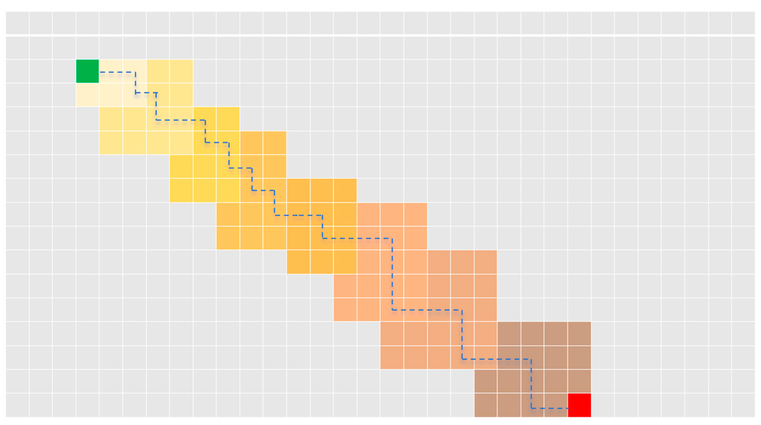
The raster map divides the 2D terrain into corresponding rasters in equal proportions, as shown in Figure 2, and the values in the rasters indicate the probability of the existence of obstacles. The main methods based on the 2D raster map are the Dijkstra method and the A* method. Takayuki Goto and Takeshi [48] investigated the application of the Dijkstra method and the A* method in intelligent transmission system and robot path planning methods and confirmed the advantages of the A* method over the Dijkstra method. Many variants of the A* method with different heuristics have emerged.
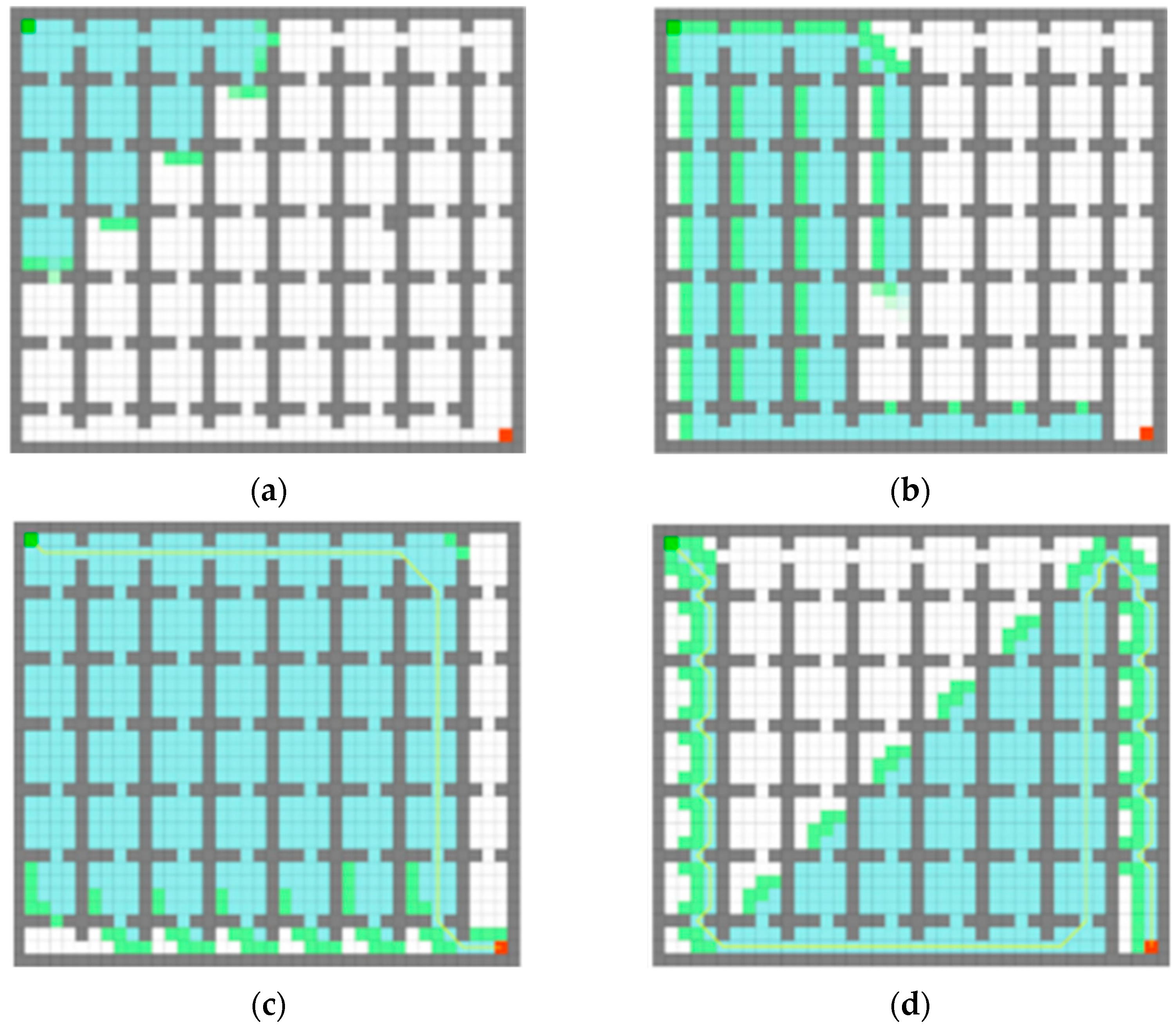
Figure 3 shows the results of the exploration process visualization of different path planning methods, revealing the differences in spatial exploration efficiency between the methods. In this case, the blue nodes represent the currently expanded parent nodes, the green nodes represent the now generated child nodes, the white nodes represent the passable regions, and the grey regions are marked as obstacle constrained spaces. To illustrate the difference between the A* method and the Dijkstra method, we give the schematic diagrams of path planning for the two heuristics, the A* method and the Dijkstra method. Figure 3a shows the path exploration process of the Dijkstra method, which needs to traverse all the nodes and is inefficient. The A* algorithm is derived from the Dijkstra algorithm by adding the Manhattan and Euclidean heuristics. These two heuristics represent the Euclidean distance or the Manhattan distance from the current position to the target point, as shown in Figure 3b,c. Figure 3d shows the breadth-first search method. However, when faced with complex scenes, the A* and Dijkstra methods have high computational overheads and the real-time performance is not very good. Although the breadth-first search method makes the exploration area smaller, the limitation of the heuristic conditions leads to the path planning is not optimal.
A heuristic function is a prediction of the cost required to proceed from the current node to the goal node, which helps to increase the search speed. Different heuristics have a different search performance. The principle is to start from the starting point, to keep traversing in the direction of the goal point, to record the parent node of each traversal point, to find the goal point, to backtrack the path, and to repeat the cycle to find the path with the minimum cost. The Euclidean inspiration allows for movement in any direction, the Manhattan inspiration is in four neighborhoods and allows for movement in four directions, up, down, left, and right.
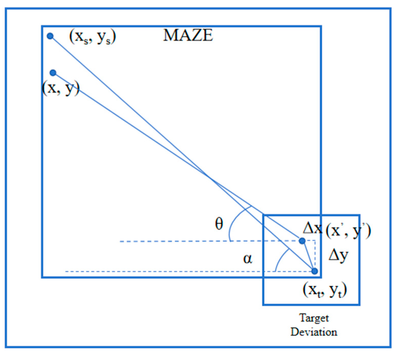
In order to select the most efficient A* method applied to mobile robots, we named the A* methods of the Euclidean and Manhattan heuristics as A* (1) and A* (2), respectively, and compared the efficiency of their searches in a simulated environment. Since the depth-first search method is basically an A* path finding method without heuristics, and thus all moves are given the same weight and are performed in a fixed order, we adopted the depth-first search method as a benchmark to evaluate the effectiveness of the heuristic function in the A* method. In the simulations, we introduced some deviations in the heuristic function for the target point orientation information of the A* method, which are shown in Figure 4. The deviation causes the search path to deviate from the optimal direction, increases the number of expanded nodes, and reduces the efficiency of the algorithm.
The cost function of the Euclidean-inspired A* (1) is as follows:
f 1 i = g 1 i + h 1 i
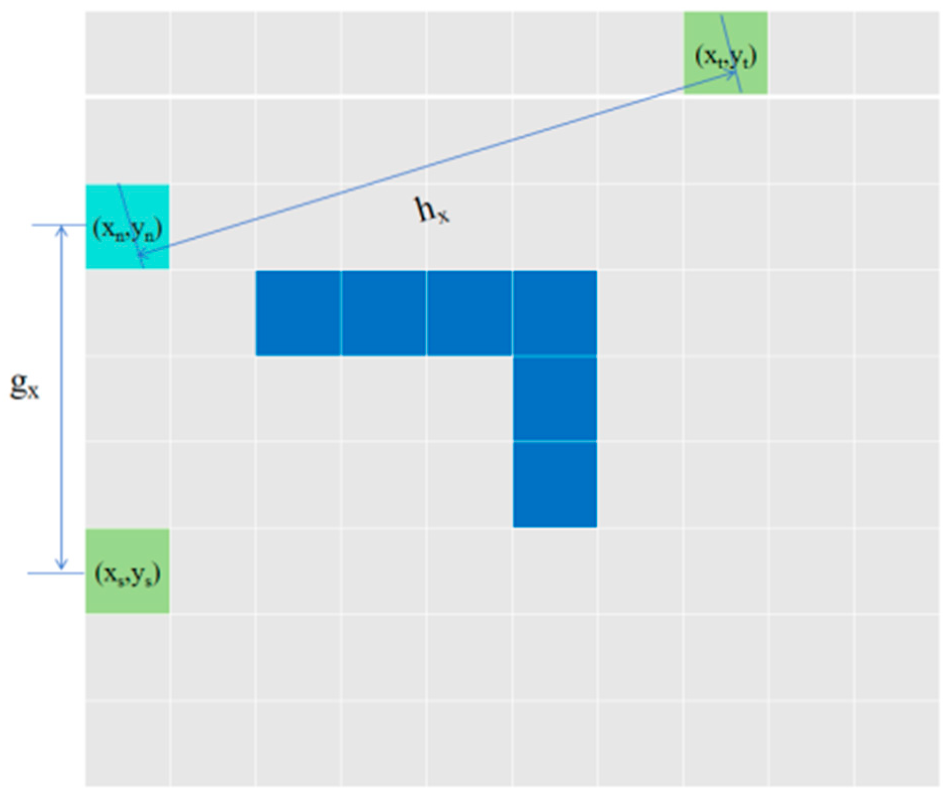
where f 1 i is the cost estimate from the starting point to the target point, i is the current position of the robot in the map, g 1 i represents the path cost function from the starting point to the current position i , and the heuristic function h 1 i represents the Euclidean distance from the current position i to the target point. Assume that the starting point is x i , y i , the middle point is x n , y n , and the target point is x t , y t . The actual distance g 1 x is denoted as follows:
g 1 x = x s x n + y s y n
For the Euclidean distance (Figure 5), the heuristic function h 1 x is expressed as follows:
h 1 x = x t x n 2 + y t y n 2
The Manhattan-inspired cost function for A* (2) is as follows:
f 2 i = g 2 i + h 2 i + h 2 j
where f 2 i represents the estimated cost from the starting point to the target point, and the heuristic function h 2 i denotes the Manhattan distance from the current position i to the target point, j is the parent point of the current point, and h 2 j is the Euclidean distance from the parent point of the current point to the target point. This term is added to the parent point to improve the search speed as it reduces the number of nodes.
For the Manhattan distance (as in Figure 6), the heuristic function h 2 i is denoted as follows:
h 2 x = x t x n + y t y n
We can obtain better results by using the Manhattan distance as the heuristic function, because the movement cost of each node is 1, and the Manhattan distance can directly estimate the movement cost between two points, and can quickly converge to the optimal solution. Using the Euclidean distance as a heuristic function may cause the search method to waste a lot of time and resources in space, may cause the search method to proceed in the wrong direction, and will need to be expanded with more nodes to find the optimal solution.

2.2.2. Cost Map

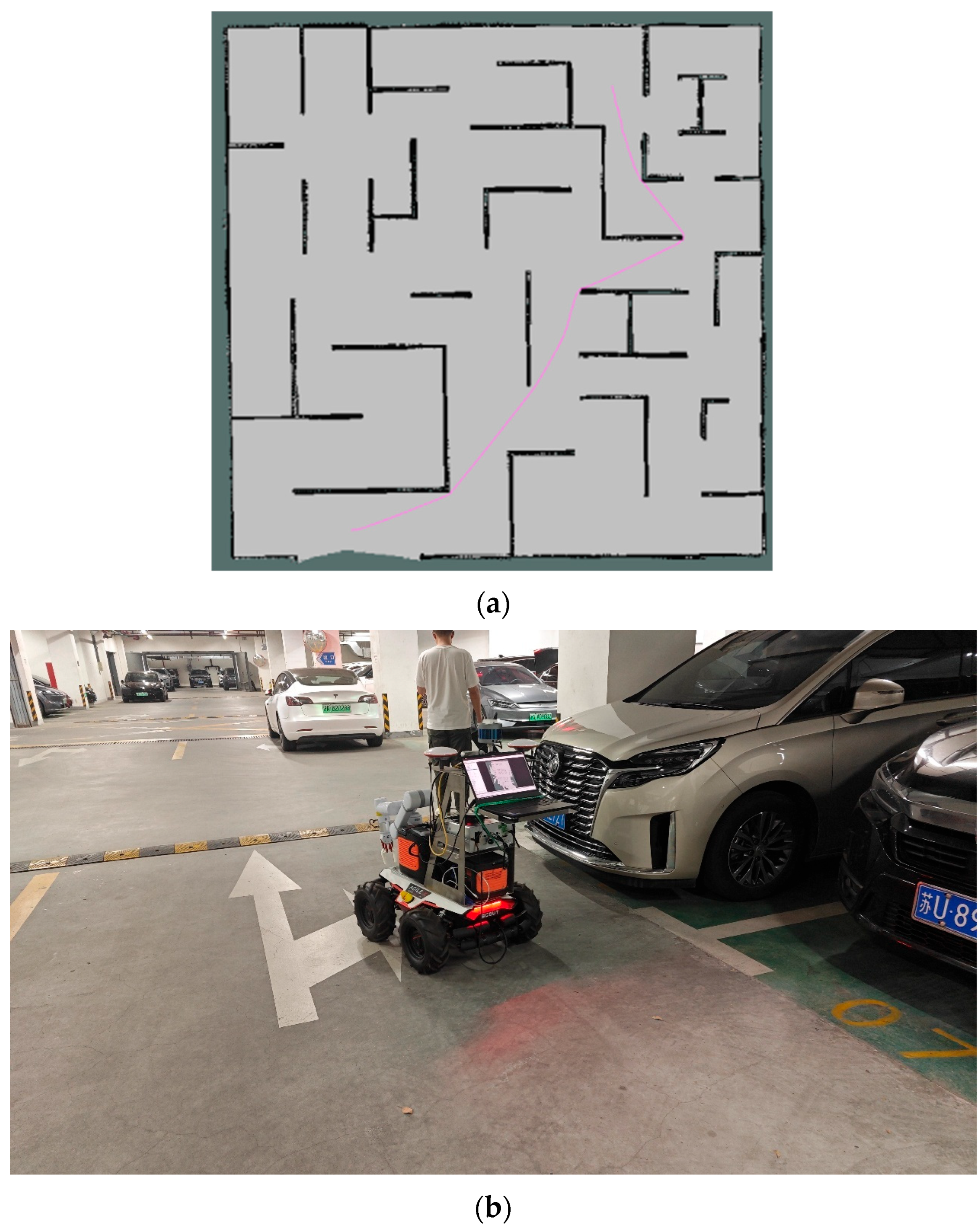
The cost map consists of a grid, cell cost is 0~255, including the three states of passable area, obstacle area, and unknown area. The cost function introduces the bicircular constraint mechanism of obstacles to achieve path optimization, establishes the geometrical model of the tangent circle and the outer circle of obstacles, and constructs the shortest path with the purpose of reaching the goal in the fastest way. However, the shortest path ignores the safe distance from the obstacles at corners and narrow sections. As shown in the visualization map in Figure 7a, white indicates passable areas, black indicates obstacle areas, and light gray represents the edges of obstacles. In this study, the A* algorithm was used to plan the red path. Since the cost function follows the principle of the shortest path and minimum cost, the algorithm tends to choose narrow passages that, in real situations, may correspond to pedestrian-only paths in underground parking lots but are obstacle areas for vehicles. In addition, the path may pass too close to obstacles, especially at corners, posing potential safety risks for vehicle movement, as illustrated in Figure 7b.

2.2.3. Layered Terrain Method

We set the surrogate value of all obstacle regions to be the same, and gradually extend it to the passable region, so that the surrogate value from the obstacle region to the passable region gradually decreases and successively realizes coarse precision and high precision path planning. We build a new cost map based on this idea, and the vehicle will consider the terrain of narrow road sections and corners as approximate obstacle areas, so as to avoid collisions. At the same time, variable scale cropping is implemented for the passable area, and the vehicle will not consider irrelevant areas for path planning, thus improving the efficiency of the path planning compared to the traditional method.
By scale transforming the original high-precision raster map to obtain the low-precision coarse raster map, the cost map of the obstacle region is set to be maximum and consistent, as shown in Figure 8. Region 2 is the gradient descent process from the obstacle region to the passable region, as an extension of the obstacle, the closer to the passable region the lower the surrogate value; the passable region is represented as the space where two gradient slopes descend below a certain height, far away from the obstacle and equidistant from the slopes, the surrogate value is equal. We will first explore the passable region and path planning. The traversal of the raster map, which is irrelevant to the A* method, can be effectively reduced by the map resolution transformation and the two-time A* method. With the improved cost map, our method is able to make the path shielded from narrow and corner sections, so that vehicles travel in the area away from the obstacles. Thus our method effectively solves the computational efficiency and shortest path safety problems faced by an underground parking lot.
Specifically, we denote the distance from the raster P i , j   to the obstacle as d P i , j , and its value is denoted as C o s t ( P i , j )   , which is abbreviated as C P :
C P = 255 d P i , j < R 255 × d ( P i , j ) I d P i , j R
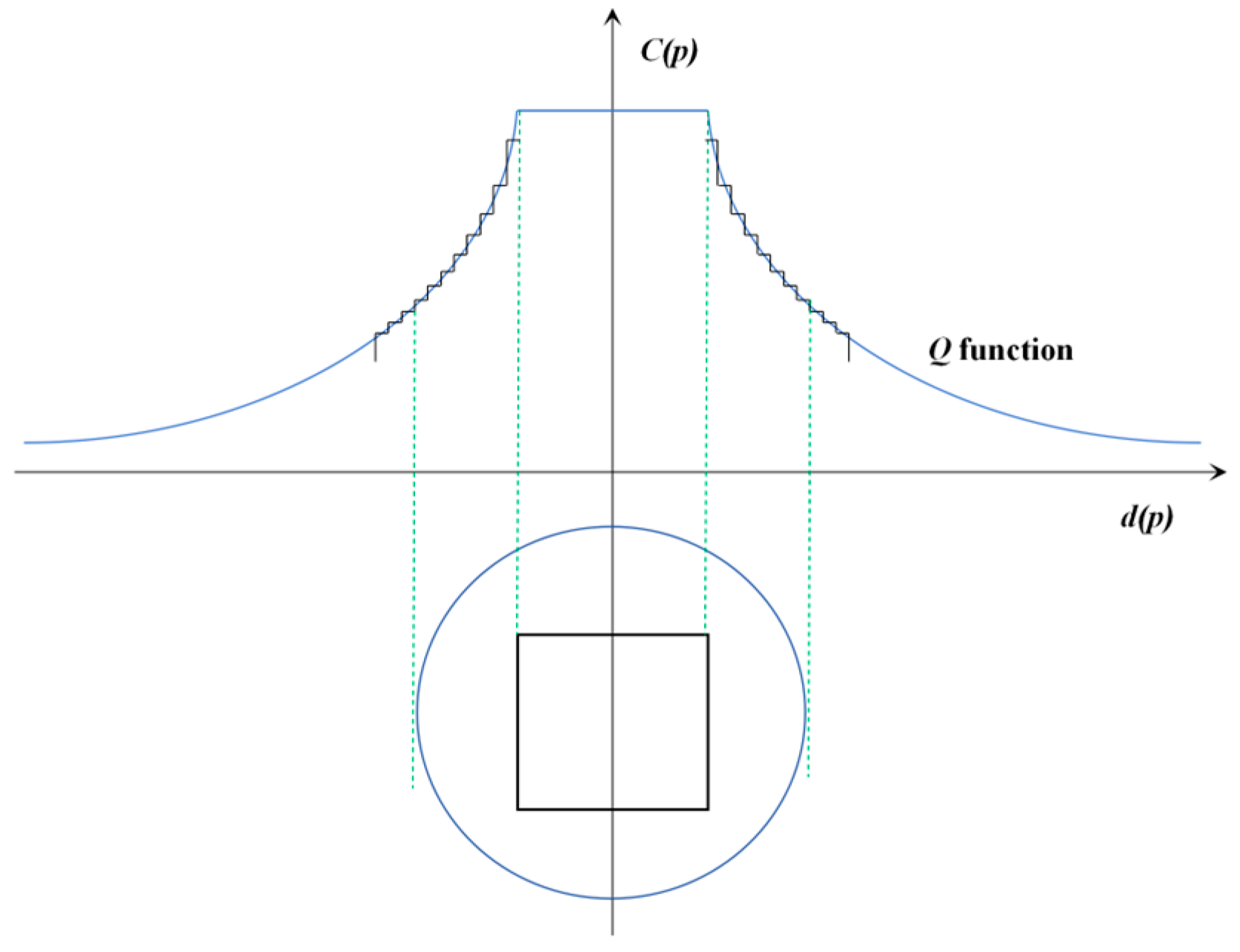
where R is the radius threshold of the obstacle, as shown in Figure 9. The raster includes an obstacle region, an unobstructed region, and an unknown region. We denote the surrogate value of the obstacle raster as 255, and the surrogate value of the unobstructed raster decreases exponentially as the distance from the obstacle raster increases.
For an accessible raster that has more than one surrogate value for different obstacle rasters at different distances, we choose the largest value as the surrogate value for that raster. Therefore, a raster with a large surrogate value has a high probability of being surrounded by obstacles and has a safety hazard, while a raster with a small surrogate value is surrounded by no obstacles, and a raster that is equidistant from two obstacles has the smallest surrogate value.
We apply the above improved cost rule to build a hierarchical cost map for underground parking lots. Firstly, we use a weighted average to transform the high-precision raster map into a low-precision raster map to build the improved cost map. The A* planning method is applied to plan the passable and accessible path planning in the coarse precision hierarchical cost map. Finally, the passable path and the surrounding domain space are reduced to the high-precision raster map as a variable-scale accessibility region, and the A* method is applied to plan global path planning only in this accessibility region.
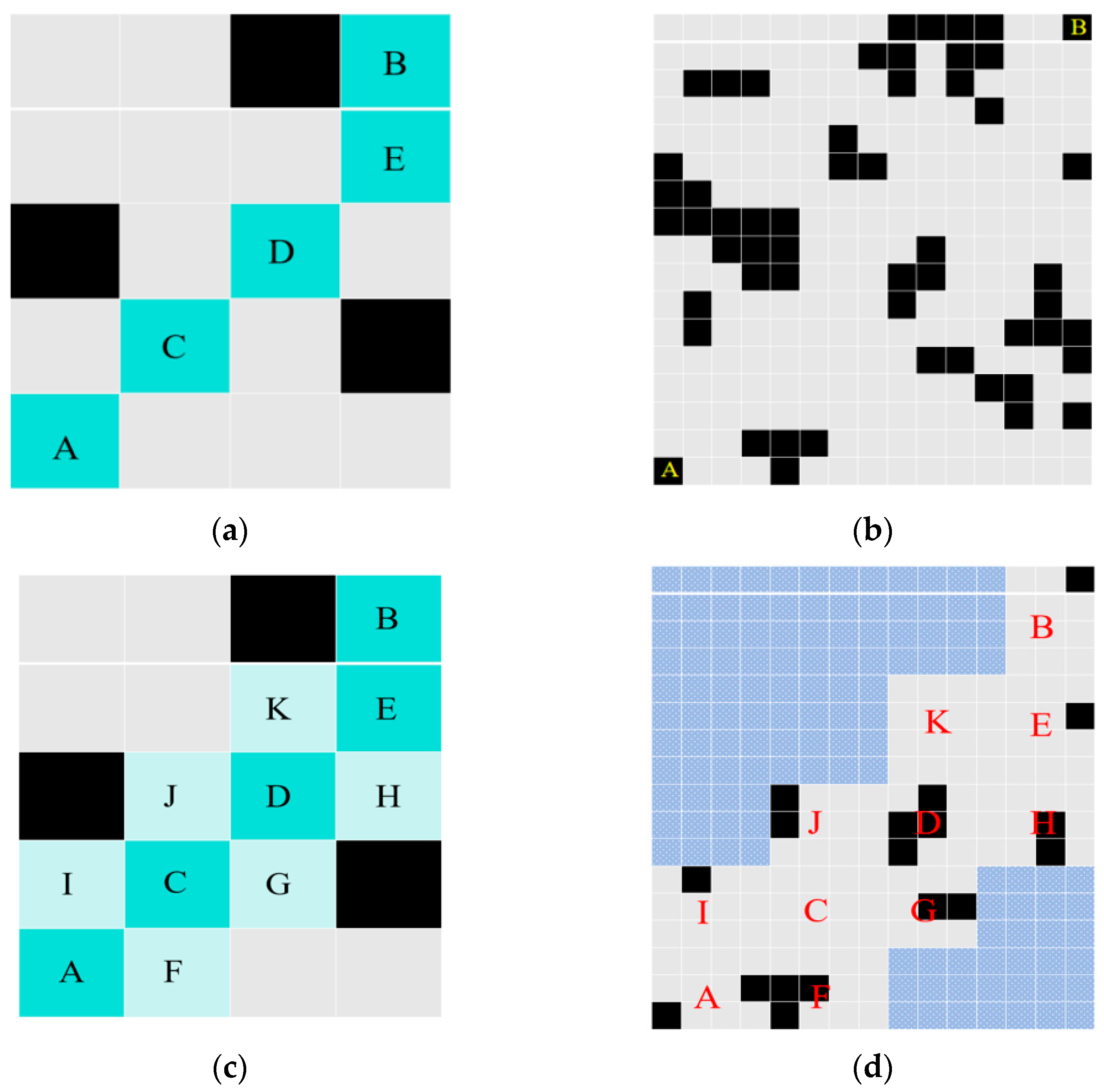
We perform variable-scale processing on the fine raster high-precision map, as shown in Figure 10a. We scale the resolution of the m × n high-precision raster map by s × t times to obtain a low-precision raster map with a resolution of m / s × n / t . For each raster a k , h in map (a), the corresponding relationship with the raster in Figure 10b is as follows:
a k , h b k s + 1 , h t + 1
And for each raster a i , j in map (b), the correspondence with map (a) is as follows:
b i , j = a s × i 1 , t × j 1 a s × i + 0 , t × j 1 a s × i 1 , t × j + 0 a s × i + 0 , t × j + 0
Specifically, define the grey value of the unobstructed raster as 206~254, the grey value of the unknown region raster as 127~205, and the grey value of the obstructed region raster as 0~126. For the grey value of the rasters in Figure 10b, the grey value of the rasters in Figure 10a will be summed and averaged within the region in Figure 10a. In Figure 10b, the rasters with grey values less than 205 are defined as obstacle regions. The process is shown below:
b i , j = k = s × i 1 , h = t × j 1 k = s × i , h = t × j a k , h s × t
b i , j = 0 b i , j < 205 255 b i , j 205
Based on the known coordinates of start point A and end point B in Figure 10b, the A* method is applied for the first time for path planning with coarse accuracy. The result is shown in the shaded part of Figure 10b, and the set of rasters through which the path passes is noted as path A-B (b).
P a t h A B b = A C D E B
To obtain the passable area, we supplement the two adjacent areas of the adjacent diagonal rasters ( i , j ) and ( i ± 1 , j ± 1 ) . For example, for rasters C and raster D in Figure 10b, they are represented by Equations (4)–(11). For the passable area around CD, the two areas J and G are added and expressed as follows:
Path A B b C D = b i , j b i ± 1 , j ± 1
Path A B b C D J G = b i , j b i , j ± 1 b i ± 1 , j b i ± 1 , j ± 1
Perform the above operation on each diagonal thick path, resulting in a passable plain area diverging from the thick path, as shown in Figure 10c, which is expressed by the following formula:
Path A B c = A C D E F G H I G K B
To obtain the passable areas in the original map, we evenly divide each raster of the passable areas in coarse-precision raster map (c) into s × t times and restore it to high-precision raster map (d). For raster c ( i , j ) Path A B , the corresponding relationship with map (a) is as follows:
c i , j = a s × i 1 , t × j 1 a s × i + 0 , t × j 1 a s × i 1 , t × j + 0 a s × i + 0 , t × j + 0
So far, we obtain the passable region in high-precision map (d). The path planning in the region is the shortest path in the global path planning. Compared with the original high-precision raster map (a), map (d) is obtained from the basis of the first A* method of path planning in the coarse-precision raster map (b). The area that is not considered in path planning is the useless blank part, and the second utilization of the A* method on this basis can make the searching area greatly reduced while retaining the original resolution, thus improving the efficiency of path planning. In the passable area for the second time using the A* method to plan the global path planning node trajectory set S = ξ i : i γ from the starting point A to the end point B, in this process you need to choose the appropriate scaling ratio based on experience, the larger the ratio, the less computation, but may lose the obstacle information, resulting in a decrease in accuracy.

2.3. Local Path Planning

To transform the global path into dynamically feasible trajectories, we combine linear interpolation with nonlinear model predictive control (NMPC). Linear interpolation generates denser nodes for smoother reference trajectories, while NMPC balances terminal cost and control cost, enabling dynamic speed adjustment in straight passages, corners, and pedestrian scenarios. Although our implementation is based on a differential-drive model, the framework can be extended to car-like robots by introducing non-holonomic constraints such as Ackermann steering geometry into the NMPC formulation, making the system suitable for real-world driverless navigation and automatic parking applications. In this study, the robot is modeled as a point for simplicity. However, the NMPC framework can incorporate geometric constraints by modeling the robot as a circle or rectangle, which would directly influence obstacle avoidance. This extension will be considered in future work to enhance realism.

2.3.1. Linear Interpolation

For autonomous navigation in underground parking lot environments, global path planning is needed to solve the computation amount and to reduce the risk of obstacle collision risk brought by the complex environment. The hierarchical terrain approach described above optimizes computational efficiency and safety; however, this process uses discrete nodes, resulting in path node generation that is not path smoothing. In addition, the vehicle operates with constant linear and angular velocities and has poor ability to cope with unexpected situations. In practical application scenarios, the vehicle cannot steer at a right angle or a flat angle, and it is necessary to control the magnitude of the vehicle steering and speed change, we hope that the vehicle encounters pedestrians or corner areas during travelling to ensure that the control action is as soft as possible, avoiding sharp acceleration and sharp turns, to ensure the safety of travelling, and accelerating in the straight area to reach the target point as quickly as possible. The path obtained by global path planning is not necessarily the local path optimization; in order to optimize the travelling route during the vehicle travelling process, we use linear interpolation and nonlinear model predictive control to obtain better local path planning.
After the global trajectory is generated, the passability on the local plane corresponding to each node is assumed to be a constant value, and the sampling step size and planning time limit the density of the generated trajectory points. To obtain denser paths, we use normalized surrogate values to represent passability and linear interpolation to achieve this. We define a dense path as follows:
S I = ξ i I τ i I : i γ I
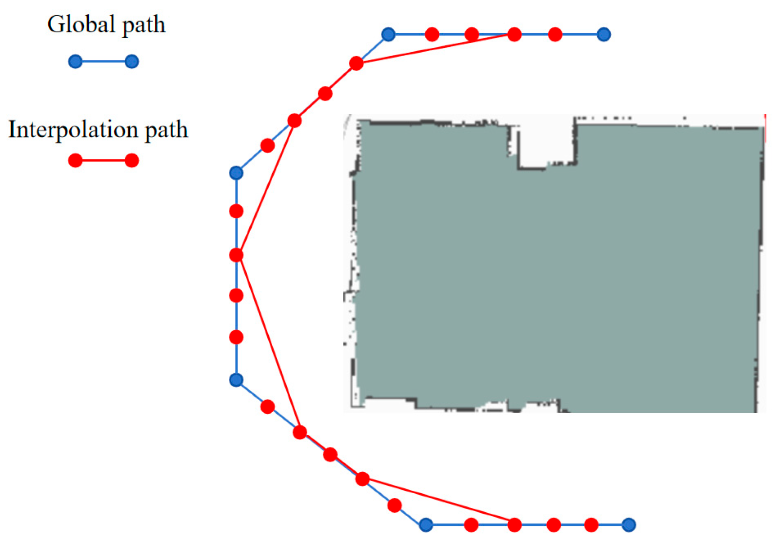
where ξ i I : i γ I is obtained from the trajectory set S = ξ i : i γ through linear interpolation. To facilitate subsequent processing, we normalize the value of the raster that the trajectory passed through to τ i I : i γ I , indicating passability. As shown in Figure 11, the vehicle global navigation results are indicated by the blue line, and the global navigation results have unnecessary redundant routes due to the sampling step problem. We construct local nodes (red) every 1 m along the route robot and connect the shortest path nodes that are directly reachable within the scanning range. The connected paths will then be added to the topology map for the calculation of the next navigation paths. It can be seen that the local path is shorter compared to the global path, and the vehicle’s path optimization has been achieved.

2.3.2. Nonlinear Control Model

In local path planning, the vehicle needs to follow the dense global path calculated by the global path planning module and linear interpolation. Denote the path nodes as S d = p i , τ i : i = 0 , 1 , , M where S d = p i , τ i : i = 0 , 1 , , M denotes the node coordinates and τ i is the map surrogate value normalized to passability.
We model local path planning as a nonlinear model predictive control NMPC problem. NMPC dynamically follows a given path using simple differential drive model dynamics, taking into account both passability and obstacle avoidance. The system acquires the vehicle state information in real time through a multi-sensor fusion framework. Specifically, the robot is aligned with a pre-built LiDAR global map, the initial pose is obtained from odometry data provided by wheel encoders, the heading angle and angular velocity are directly measured by the inertial measurement unit (IMU), and the final pose is estimated through sensor fusion of LiDAR matching results, odometry data, and IMU measurements. The optimization problem contains N nodes and, to simplify the problem, we use a differential drive model on the local plane as the system model:
x k + 1 y k + 1 θ k + 1 = x k y k θ k + cos θ k 0 sin θ k 0 0 1 u k Δ t
The optimization formulation is shown below:
min x k u k k = 0 N 1 x k x k Q d 2 + λ u k R 2
s . t . x k + 1 = f x k , u k
x 0 = x start
x k X , u k U
x k x i o b d safe
where X represents the set of target points, U represents the set of control quantities, and x k d represents the target points, which are obtained through S d . x A : = 0.5 x T A x . The two positive definite matrices Q and R are the coefficients for measuring the terminal cost and control cost, respectively. λ = 1 t m e a n 2 is the control cost coefficient, and t m e a n is obtained by averaging τ i over the current local area. This coefficient can help the robot slow down when the average passability is poor or the estimated confidence level is low. u k is the control input vector of the differential drive model at time step k , and the linear velocity component v k controls the forward/backward speed of the robot in the current direction θ k . The angular velocity component ω k controls the steering speed of the robot, which represents the rotational speed of the vehicle around its vertical axis, updated from θ k to θ k + 1 . In the objective function, u k penalties control the input costs, such as energy consumption and motor torque, and λ serves as a coefficient to force u k to reduce the linear speed and angular speed on terrain with poor passability (such as encountering pedestrians and corners) to enhance safety, while on terrain with good passability, attention is focused on the terminal cost to force the vehicle to reach the target position faster. Therefore, the local path planning we designed, on the basis of smoothly optimizing the path, takes into account the dynamic control of vehicles according to terrain differences, balances safety and efficiency, and achieves the coordinated optimization of safe obstacle avoidance, terrain adaptability and motion efficiency.

3. Results

3.1. Experimental Details

All experiments in this paper were conducted under the following parameter configurations: the original map resolution was 500 × 500 pixels, and the coarse-resolution map was 50 × 50 pixels; the heuristic function of the A* algorithm was set to the Manhattan distance with a cost weight of λ = 0.6 ; the NMPC parameters included a prediction horizon of N = 20 , a sampling time of Δ t = 0.1 s, and weighting matrices Q = d i a g ( 1 , 1 , 0 , 5 ) and R = d i a g ( 0.1 , 0.1 ) ; the simulation platform used ROS Melodic and Gazebo 9.0; the real vehicle sensors included a Velodyne VLP-16 LiDAR (Velodyne Lidar Inc., San Jose, CA, USA) and wheel encoders.

3.2. Qualitative Experiment on the Simulation Platform

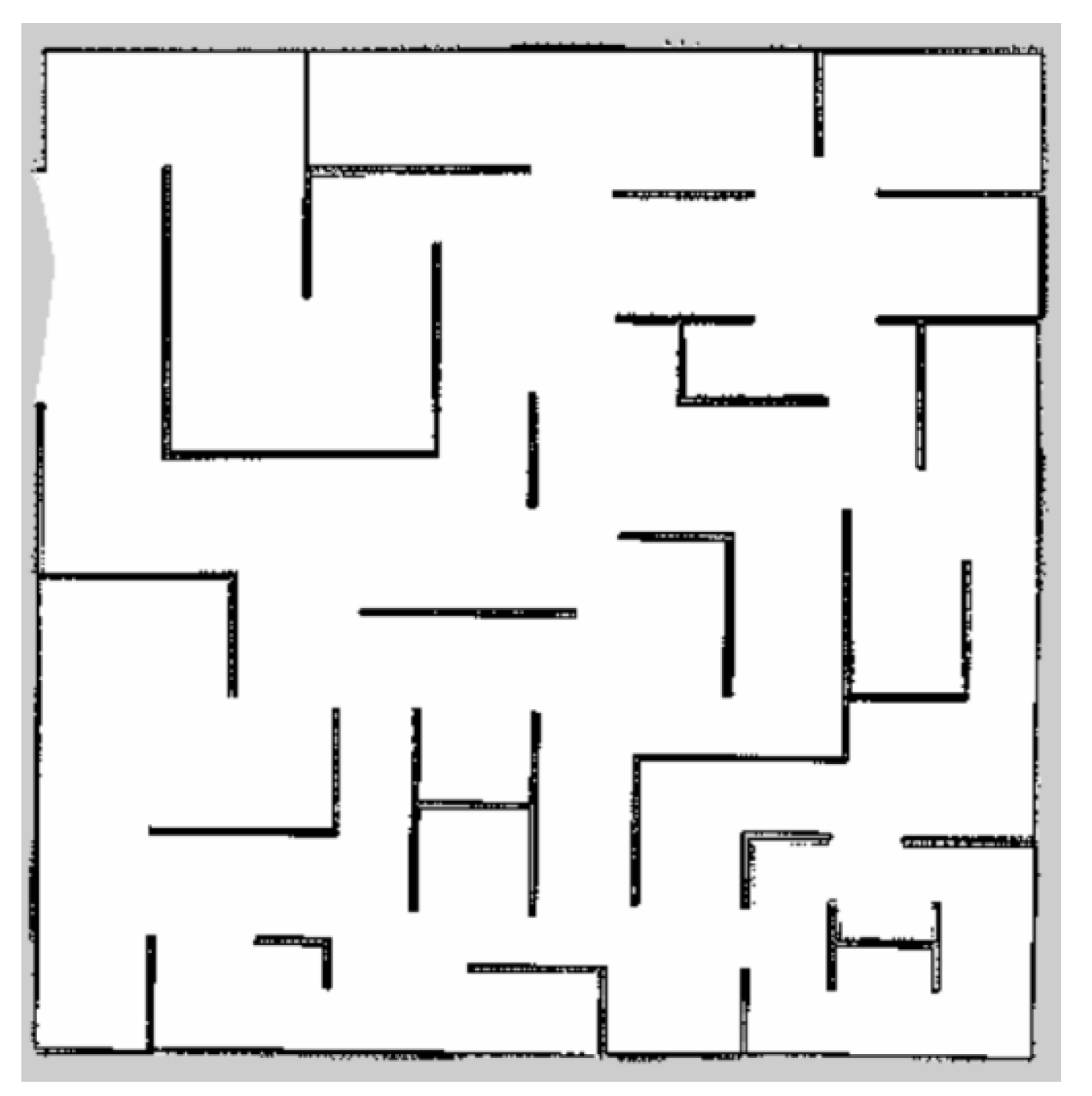
To verify the reliability of our method, a 2D raster map was first built in a benchmark environment on the simulation platform to run the proposed global path planning algorithm. This map retains the static structural features of the real environment and is used to evaluate the performance of the global path planning method. Figure 12 shows the raster map constructed from LiDAR point cloud data. The original high-resolution raster map (500 × 500 pixels) is transformed into a scale space, and a 10 × 10 window is used to generate binarized grey values by weighted averaging of the rasters in the region, resulting in a coarse-precision raster map, as shown in Figure 13, which consists of obstacle areas (black) and passable areas (white).
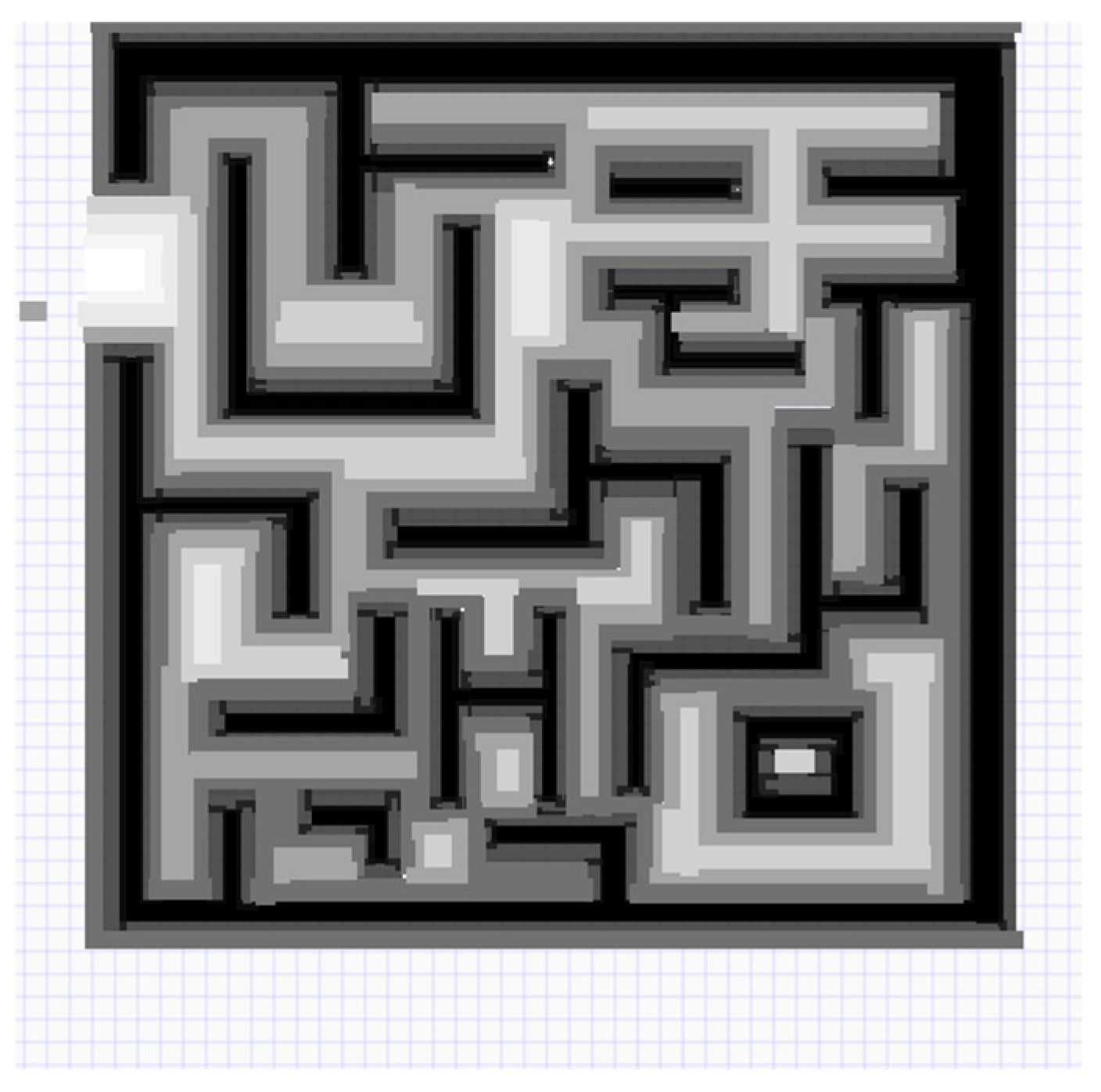
We continue to extend the obstacle regions by the improved cost map with the gradient extension to obtain the coarse accuracy cost map shown in Figure 14. Where the raster grey value (0~255) is the surrogate value, reflecting the degree of raster proximity to the obstacle, showing a smooth transition from the fully passable area (white) to the obstacle area (black). This approach effectively preserves the topological features of the real environment.
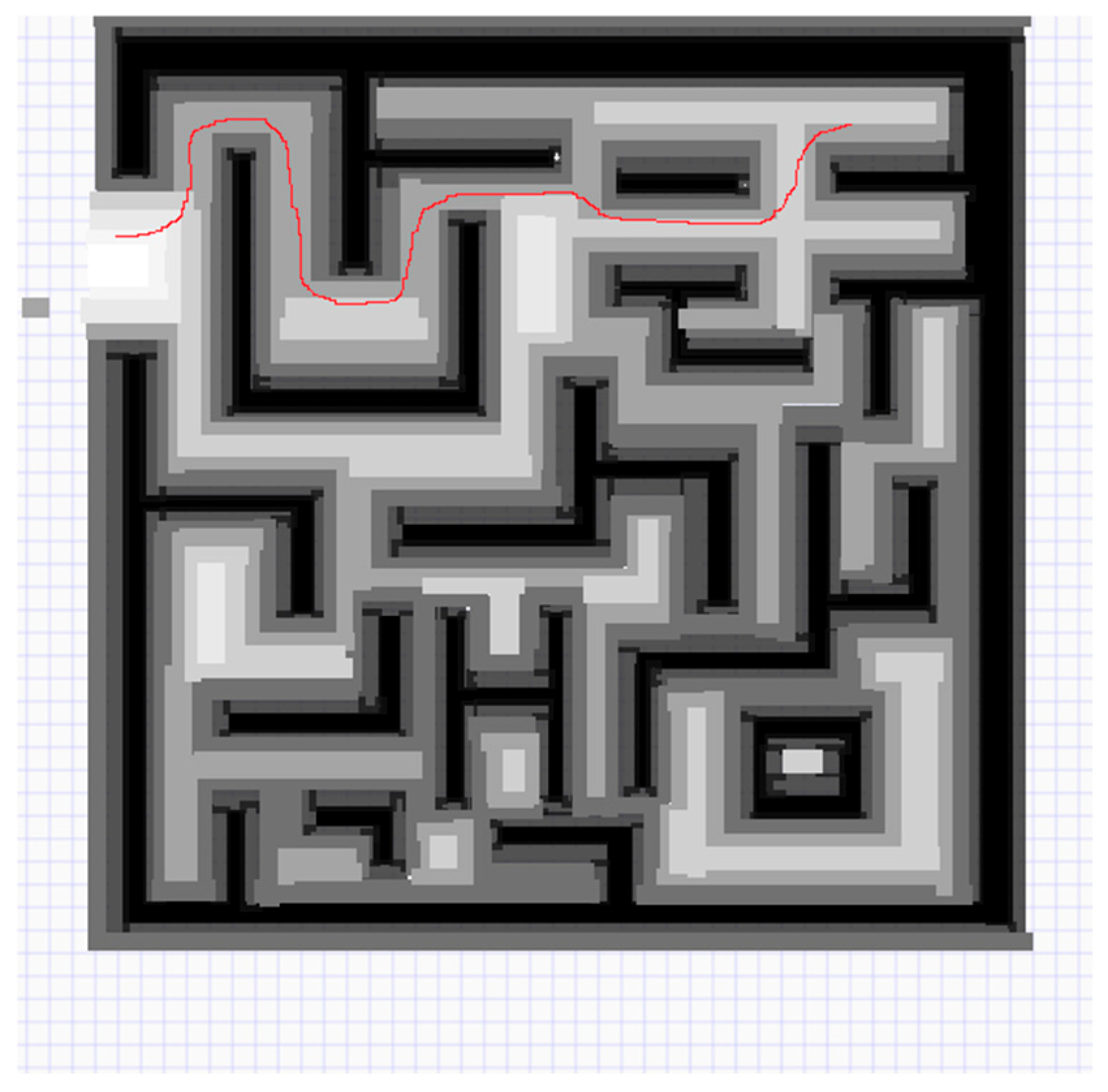
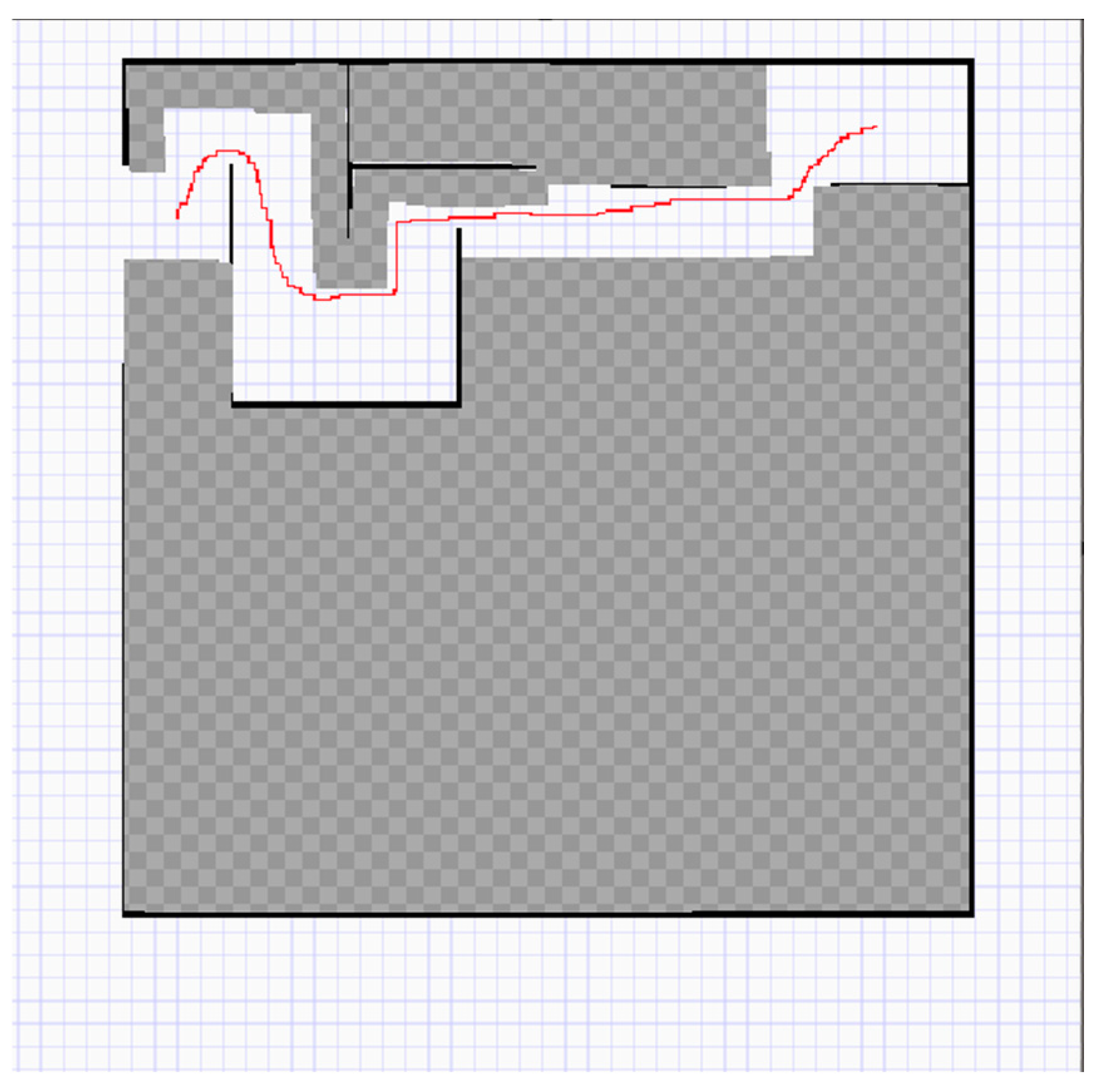
Figure 15 represents the initial path (red trace) generated using global path planning in a coarse resolution raster map, where the path follows the principle of staying away from obstacle areas and the gradient portion of the hierarchical terrain cost map, maintaining a sufficient distance from obstacles and exhibiting significant safety. By reverse mapping this coarse-grained path to the original high-precision map, a sufficiently safe traversal area is obtained (Figure 16, white area). It is worth noting that this path optimization search space only accounts for a relatively small percentage of the full map area of the original high-precision raster map, yet retains the range of the global optimal solution’s existence intact. Therefore, subsequent implementation of the A* method only on this area will greatly reduce the number of nodes to be traversed. The red trace in Figure 16 shows the final global path. The above results fully validate the advantages of our proposed hierarchical terrain approach. With this two-stage processing strategy, the system not only ensures the path security, but significantly reduces the computational complexity, which is suitable for dealing with real-time path planning problems in large-scale environments, and provides a new technological idea for solving the navigation problems of mobile robots in complex environments.
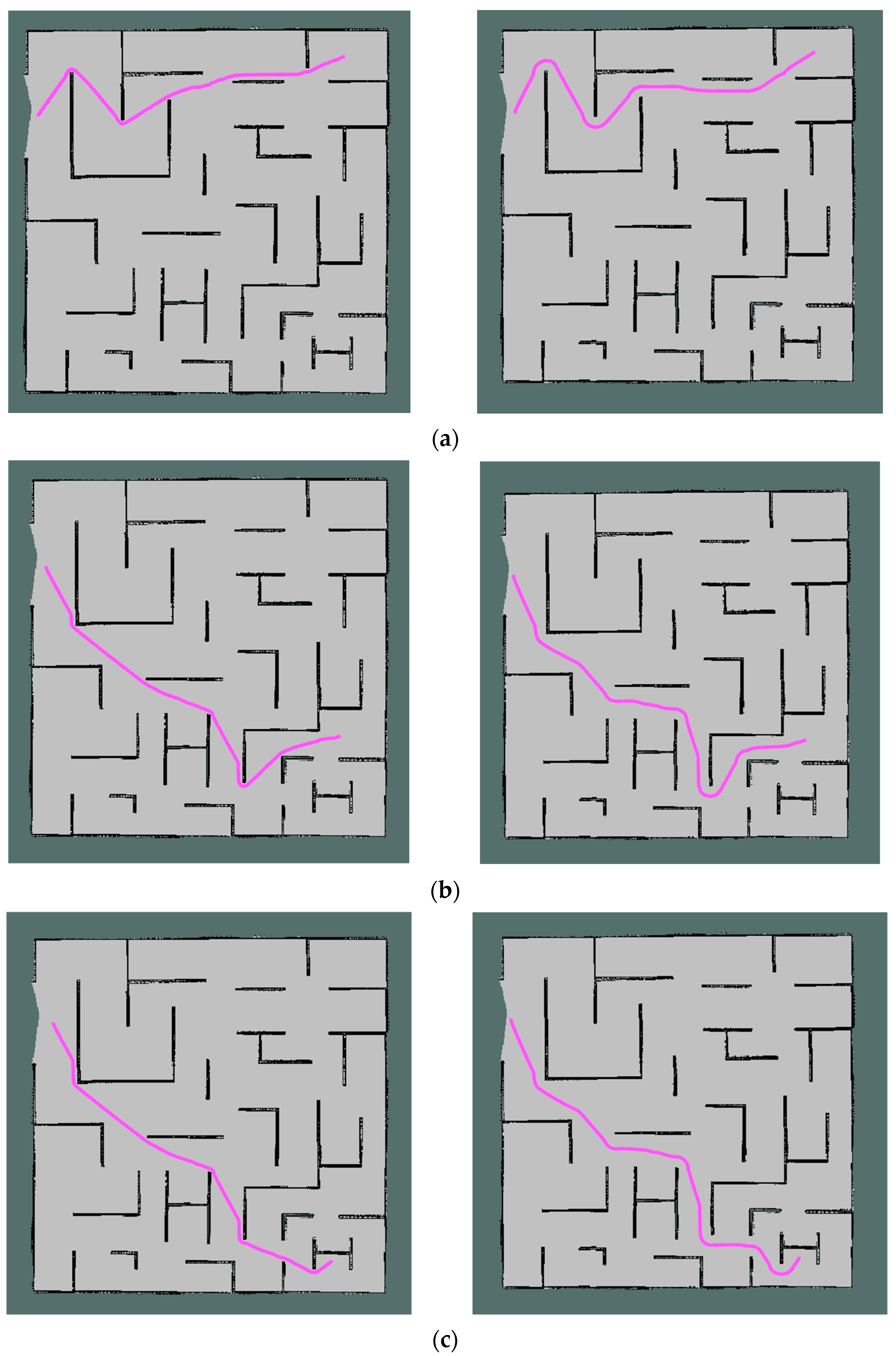
To further highlight the advantages of our method, we changed the current and target positions and conducted multiple experiments to compare the path planning results of the traditional A* [49] algorithm with those of the proposed layered terrain algorithm. As shown in Figure 17a–c, the results indicate that our layered terrain algorithm guides the path away from obstacles through the hierarchical cost map. Although the path length slightly increases, navigation safety is significantly improved. By contrast, the traditional A* algorithm pursues the shortest path, causing the trajectory to pass very close to obstacles in corners and narrow areas, which increases the risk of collision.
It is worth noting that our proposed layered terrain method differs fundamentally from the traditional wall dilation approach. Wall dilation typically applies a uniform morphological expansion around obstacles, producing fixed buffer zones with constant safety margins. By contrast, the layered terrain cost map establishes a gradient-based cost field in which surrogate values gradually decrease from obstacle regions to passable areas. This creates multiple terrain layers that guide the planner to select paths adaptively based on local terrain variations rather than simply avoiding inflated walls. As illustrated in Figure 17, this strategy achieves smoother trajectories with stable obstacle clearance, balancing safety and computational efficiency more effectively than uniform wall dilation.

3.3. Simulation Platform Ablation Experiment

Meanwhile, in order to illustrate the computational efficiency of our method, the original A* method is quantitatively compared with the layered terrain method, comparing the total path length, proximity to obstacles, and the method running time. As shown in Table 1, although the hierarchical terrain method does not take the shortest path and the path length is only slightly increased compared to the A* Method, the actual running time is shorter than the A* method, which results in higher computational efficiency, and the path planning computational Efficiency does not show any proximity to obstacles, which improves the safety.
We add the local path planning method to the global path planning method to achieve dynamic adjustment during vehicle operation. The effect of adding the local path planning method on autonomous navigation process is shown in Table 2, which records the running time in the total running time and the running time on each road section. From the data in Table 2, it can be seen that the local path planning method can be used in the straight ahead area with less running time, pursuing smaller terminal cost to achieve higher speed and faster arrival at the target point; and can be used in the corner area with a longer running time, pursuing smaller control cost to achieve more stable control and safety. The method with the addition of local path planning is less in total running time.

3.4. Experiments in Real Scenes

In this subsection, based on the scene reconstruction method proposed in this Section, the collected dataset is used to construct a 3D map, which is further converted into a structured 2D planar map for method testing and evaluation. On this basis, we carry out systematic validation of the proposed method around this 2D map, focusing on evaluating its path planning effect and autonomous navigation performance in complex dynamic scenes.
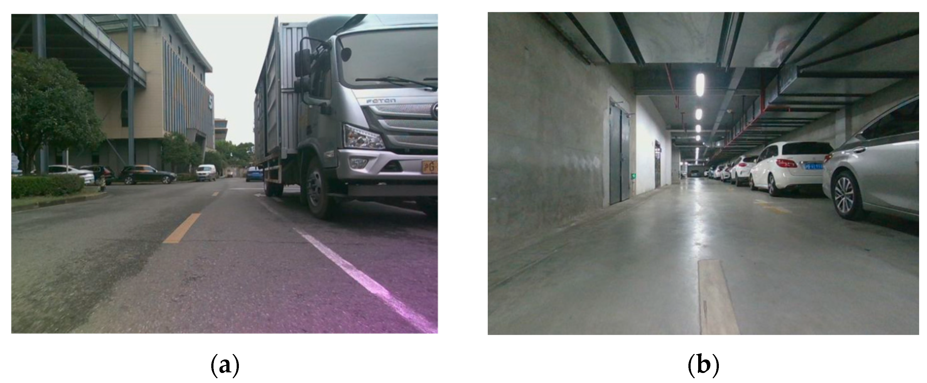
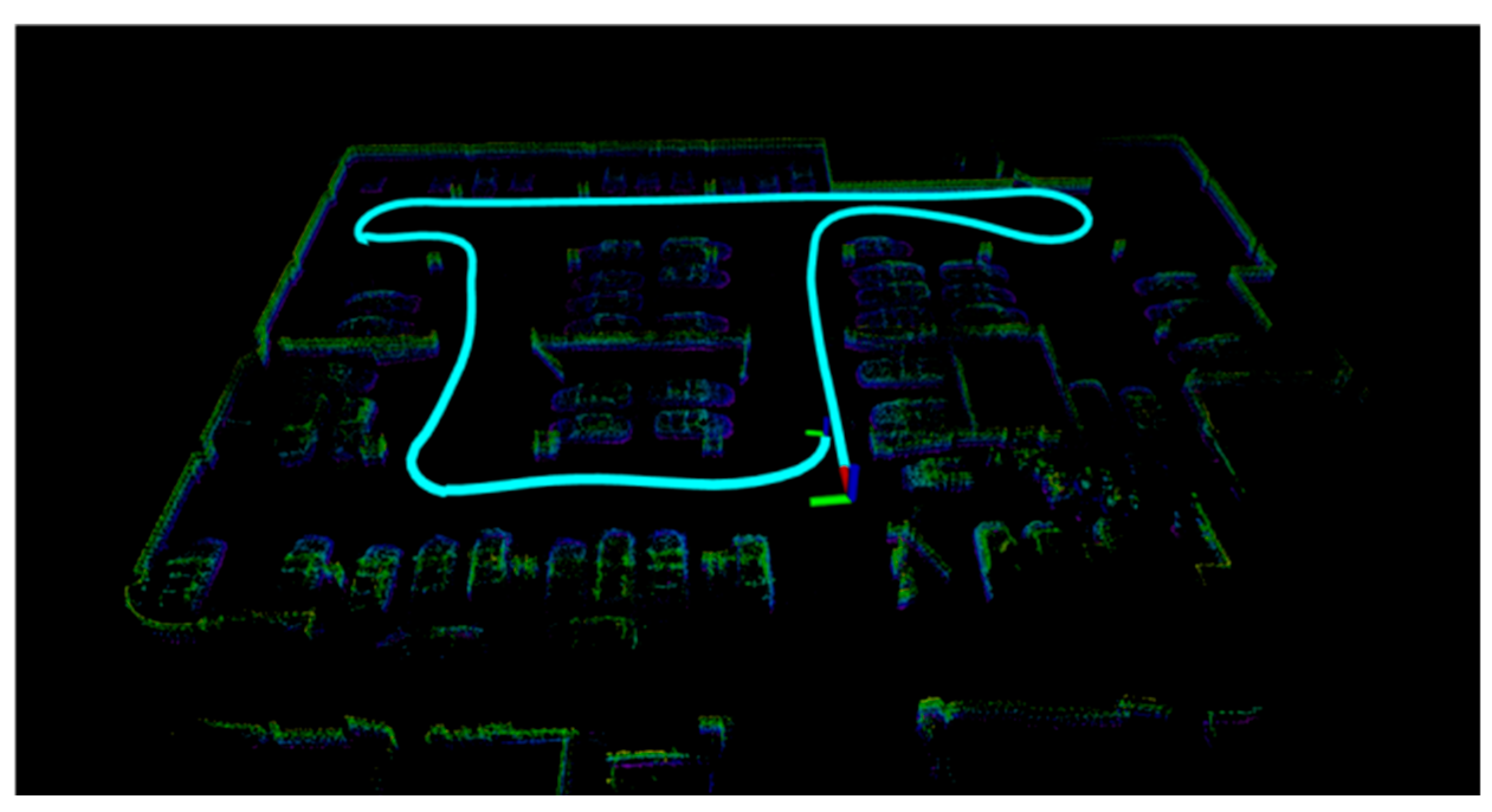
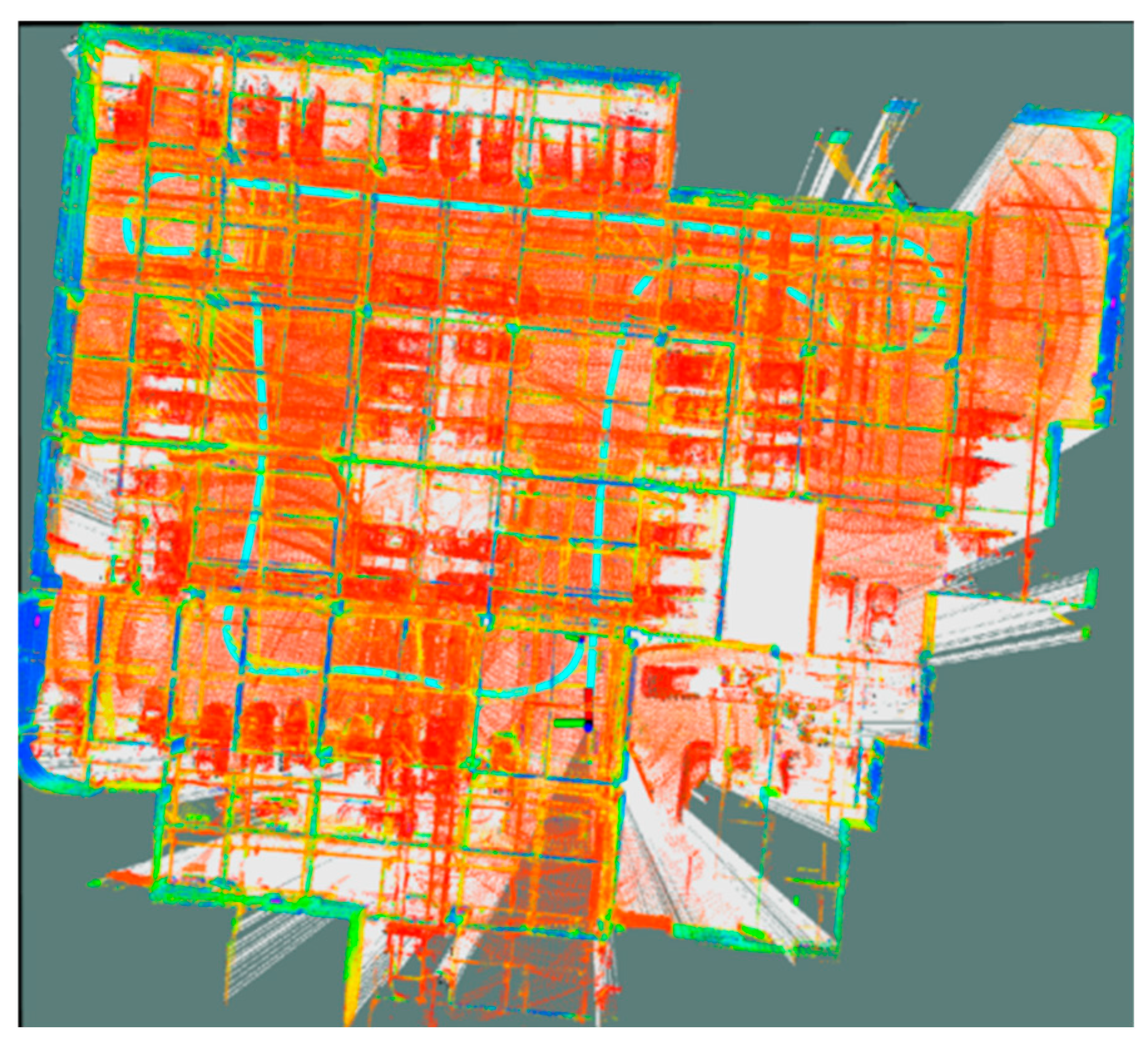
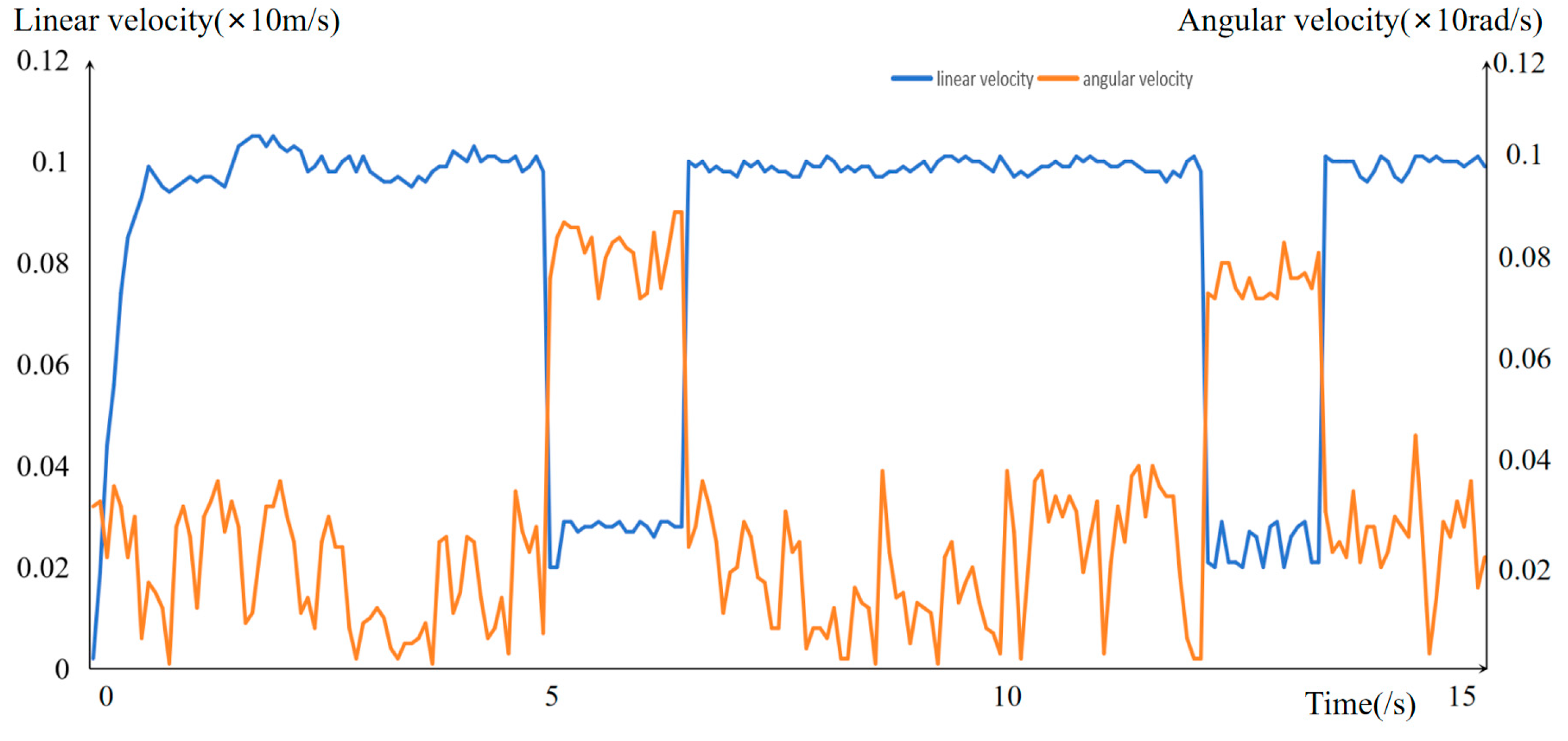
In this paper, the real scene of an urban industrial park is shown in Figure 18. The left figure is the part above ground, and the right figure is the underground parking lot. Since the environment of underground parking lot is more complex, we take underground parking lots as an example to show the navigation results. Firstly, the 3D mapping of the underground parking lot is carried out. The result is shown in Figure 19, and the constructed 3D point cloud map is shown in Figure 20. After constructing the original map, the global and local path planning methods are used to solve the problem. The results are shown in Figure 21. By adding the terminal cost and control cost to NMPC, the vehicle’s linear and angular velocities decrease during turning and obstacle avoidance, while both accessibility and velocity increase during diameter, achieving the effect of dynamic speed adjustment of the vehicle in different accessibility terrains. In this study, the linear and angular velocities of the vehicle during operation are recorded in Figure 22 to demonstrate the control process of our method in controlling the vehicle during local path planning. It can be seen that the linear velocity of the vehicle decreases and the angular velocity increases at the two corners, while the linear velocity increases and the angular velocity decreases in the unobstructed straight ahead area.
Unlike the simulation environment, the underground parking lot environment needs to consider the influence of pedestrians, among other factors. In order to verify the practicality of the local path planning method in real scenarios, the sudden appearance of pedestrians is added to the paths shown in Figure 21, and the runtimes of the global path planning method and the global + local path planning method in the three types of terrains are compared, as shown in Table 3. Compared with the navigation process with only global path planning, our approach takes 1.68 s more time in the corner region, which is attributed to the local path planning approach pursuing smaller control cost to achieve more stable control and safety, and 0.89 s less time in the straight ahead region, which is attributed to the local path planning approach pursuing smaller terminal cost to achieve fast approach to the target point. When encountering the sudden appearance of pedestrians, our approach can quickly adjust the navigation strategy to avoid collision, and the time to avoid pedestrians increases by 3.58 s, the vehicle pursues higher safety. In terms of total running time, our method takes 4.37 s less time, which is more efficient overall. Figure 22 shows the real-time linear and angular velocities of the vehicle during the running process.
Meanwhile, we compare the running time of local path planning baseline methods, such as the A* [33], PSO [45], ACO [46], ABC [47], RRT* [50] method, the PF-RRT* [51] method FL [52], and the CSA [53] method, for the three types of terrain, and the passable straight ahead area, the corner area, and the pedestrian times are compared. We use the layered terrain method as the other baseline method for global path planning. In order to demonstrate the advantages of our methods in terms of response time, the baseline methods are applied directly to a real scenario of a gridded map for an underground parking lot, and the point cloud data was analyzed using the same methods. The same starting and ending points are chosen for each method. The performance of each method is evaluated using the optimal solution time metric. Considering that sample-based methods are not guaranteed to find the optimal solution, the experiment compares the time cost of the four methods in path optimization. Table 4 shows the results.
Table 4 shows that, in the straight area, our method takes 7.01 s, which is the least time consuming, compared to the PF-RRT* method, which is reduced by 0.51 s; the ACO method takes the most time at 8.74 s. In the turning area and the encounter with pedestrians, our method takes into account the safety of the vehicle and reduces the speed of the vehicle in order to avoid the collision, which takes the most time at 4.73 s and 3.42 s, respectively. The RRT* method uses a tree search structure because it obviously increases a lot of computational time consumption, with a total time consumption of 15.29 s, while our method has a minimum of 15.16 s in total time consumption. The PF-RRT* method reduces the terrain analysis by focusing on the possible passing terrain only. The FL method has high memory requirements, and the rules and parameters require human intervention to a large extent. The PSO method has a slow convergence in the late stage, and it is easy to fall into a local optimum. The CSA method cannot guarantee a global optimal solution. For more complex solutions, it is not possible to guarantee an optimal solution for the vehicle optimal solution, and it is less effective for more complex or larger problems. The ABC method is time-consuming in parameterization and fine-tuning, and has high memory requirements. The ACO method has slow early convergence. In different scenarios, it is necessary to consider the accuracy and convergence speed of the method. Our method is capable of dynamic speed adjustment in different situations, it takes the shortest time in the straight ahead region, and it keeps away from and decelerates when passing through corners and encountering pedestrians, which is optimal in terms of computational efficiency, speed, and safety. Figure 23 shows the path planning of the vehicle when a pedestrian is detected.
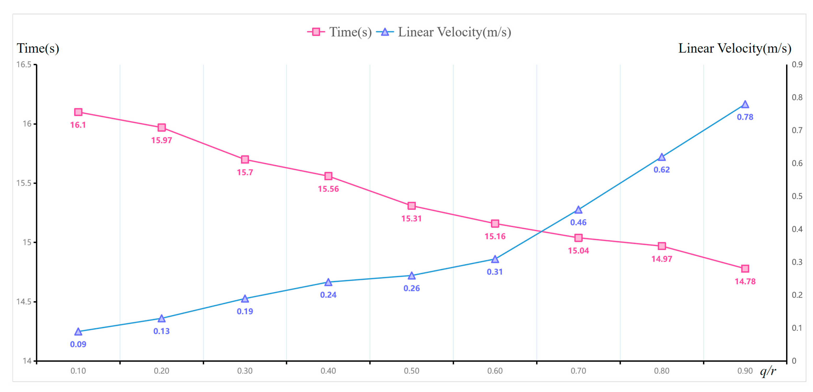
For the state weight matrix Q and the control weight matrix R in the objective function of local path planning, we set the diagonal vectors of the matrices to be equal constants, q and r, respectively. There is a conflict between reaching the target position quickly and reducing the control cost. In order to weigh the control cost and the terminal cost and to determine the optimal loss weight configuration, we calculate the total running time and the average value of linear velocity when encountering obstacle avoidance by pedestrians for the method in the three terrain situations with different weight configurations q/r. The results are shown in Figure 24, with the horizontal axis denoting q/r, the left vertical axis denoting the total running time, and the right vertical axis denoting the linear velocity. The results show that, when q/r is set smaller, the function focuses on respecting the control cost, and the vehicle operation control is stable but consumes a long time; when q/r is set larger, the model focuses on the terminal cost, and the vehicle will arrive at the target point quickly but encounters pedestrians with poor deceleration effect, which is a potential safety hazard. We set q/r to 0.6 to make the vehicle control stable under the guarantee that the running time is shorter than the baseline method in advance.

4. Conclusions

Aiming at the current problems of computational efficiency and insufficient security in robot autonomous navigation, we design hierarchical terrain global path planning and nonlinear model prediction-based local path planning. For the inefficiency of the current A* method, we adopt the coarse accuracy path planning of the coarse accuracy cost map as a premise and implement the A* method in the pre-planned area, which reduces irrelevant node traversal and improves computational efficiency. In order to improve safety, we design the hierarchical terrain cost map principle and construct an improved cost map to realize that the vehicle can avoid a collision risk in narrow passages and corners. In order to achieve the dynamic adjustment of the vehicle in different terrains, we propose a combination of nonlinear model and linear interpolation, in accordance with the differential drive model to path optimization of terminal cost and control cost, to ensure the local optimum of the vehicle path. Quantitative and qualitative experiments are conducted in an underground parking lot with complex conditions, and the results show that our method outperforms the A* method in computational efficiency, is able to avoid collision risk by staying away from pedestrians and walls, among other obstacles, and is capable of dynamic speed adjustment for different terrains. It outperforms all the baseline methods in terms of comprehensive performance.
Nevertheless, we recognize certain limitations. In this study, the robot is simplified as a point for path planning. In future work, the framework can be enhanced by modeling the vehicle as a circular or rectangular rigid body, so that its geometric dimensions directly constrain the traversable area. This will allow a more realistic representation of vehicle–obstacle interactions and further strengthen the applicability of our method to real-world autonomous driving and automatic parking tasks.
In addition, we plan to further improve the optimization efficiency of our framework. Since gradient descent is used in the cost optimization process, it would be valuable to investigate accelerated gradient descent or adaptive optimization algorithms (e.g., Nesterov acceleration or Adam variants) to enhance convergence speed and global stability. Future studies will also focus on extending the proposed approach to more dynamic and unstructured environments, integrating real-time perception, and improving adaptability in large-scale navigation scenarios.

Author Contributions

W.C.: conceptualization, methodology, writing—original draft. L.H.: investigation. S.S.: investigation. Y.W.: investigation. Q.P.: writing—review and editing. X.M.: writing—review and editing. All authors have read and agreed to the published version of the manuscript.

Funding

This research was funded by the National Natural Science Foundation of China under Grant 62306128, the Basic Science Research Project of Jiangsu Provincial Department of Education under Grant 23KJD520003, the Leading Innovation Project of Changzhou Science and Technology Bureau under Grant CQ20230072, and the National Key Research and Development Program of China under Grant 2023YFF1105102.

Institutional Review Board Statement

Not applicable.

Informed Consent Statement

Not applicable.

Data Availability Statement

Dataset are available upon request from the authors.

Conflicts of Interest

The authors declare that they have no known competing financial interests or personal relationships that could have appeared to influence the work reported in this paper.

References

  1. Huang, C.; Mees, O.; Zeng, A.; Burgard, W. Visual language maps for robot navigation. In Proceedings of the 2023 IEEE International Conference on Robotics and Automation (ICRA), London, UK, 29 May–2 June 2023; IEEE: New York, NY, USA, 2023; pp. 10608–10615. [Google Scholar]
  2. Wang, C.Y.; Bochkovskiy, A.; Liao, H.Y.M. YOLOv7: Trainable bag-of-freebies sets new state-of-the-art for real-time object detectors. In Proceedings of the IEEE/CVF Conference on Computer Vision and Pattern Recognition, Vancouver, BC, Canada, 17–24 June 2023; pp. 7464–7475. [Google Scholar]
  3. Liu, S.; Zeng, Z.; Ren, T.; Li, F.; Zhang, H.; Yang, J.; Jiang, Q.; Li, C.; Yang, J.; Su, H.; et al. Grounding dino: Marrying dino with grounded pre-training for open-set object detection. In Proceedings of the European Conference on Computer Vision, Milan, Italy, 29 September–4 October 2024; Springer Nature: Cham, Switzerland, 2024; pp. 38–55. [Google Scholar]
  4. Tzafestas, S.G. Mobile robot control and navigation: A global overview. J. Intell. Robot. Syst. 2018, 91, 35–58. [Google Scholar] [CrossRef]
  5. Ginting, M.F.; Kim, S.K.; Fan, D.D.; Palieri, M.; Kochenderfer, M.J. Seek: Semantic reasoning for object goal navigation in real world inspection tasks. arXiv 2024, arXiv:2405.09822. [Google Scholar] [CrossRef]
  6. Gadd, M.; Newman, P. A framework for infrastructure-free warehouse navigation. In Proceedings of the 2015 IEEE International Conference on Robotics and Automation (ICRA), Seattle, WA, USA, 26–30 May 2015; IEEE: New York, NY, USA, 2015; pp. 3271–3278. [Google Scholar]
  7. Ackerman, E. A Robot for the Worst Job in the Warehouse: Boston Dynamics’ Stretch can move 800 heavy boxes per hour. IEEE Spectr. 2022, 59, 50–51. [Google Scholar] [CrossRef]
  8. Shiomi, M.; Kanda, T.; Ishiguro, H.; Hagita, N. Interactive humanoid robots for a science museum. In Proceedings of the 1st ACM SIGCHI/SIGART Conference on Human-Robot Interaction, Salt Lake City, UT, USA, 2–3 March 2006; pp. 305–312. [Google Scholar]
  9. Huang, C.M.; Iio, T.; Satake, S.; Kanda, T. Modeling and Controlling Friendliness for An Interactive Museum Robot. In Proceedings of the Robotics: Science and Systems, Berkeley, CA, USA, 12–16 July 2014; pp. 12–16. [Google Scholar]
  10. Hossain, M. Autonomous delivery robots: A literature review. IEEE Eng. Manag. Rev. 2023, 51, 77–89. [Google Scholar] [CrossRef]
  11. Vaussard, F.; Fink, J.; Bauwens, V.; Rétornaz, P.; Hamel, D.; Dillenbourg, P.; Mondada, F. Lessons learned from robotic vacuum cleaners entering the home ecosystem. Robot. Auton. Syst. 2014, 62, 376–391. [Google Scholar] [CrossRef]
  12. Xiao, X.; Liu, B.; Warnell, G.; Stone, P. Motion planning and control for mobile robot navigation using machine learning: A survey. Auton. Robot. 2022, 46, 569–597. [Google Scholar] [CrossRef]
  13. Elfes, A. Using occupancy grids for mobile robot perception and navigation. Computer 2002, 22, 46–57. [Google Scholar] [CrossRef]
  14. Filliat, D.; Meyer, J.A. Map-based navigation in mobile robots: I. a review of localization strategies. Cogn. Syst. Res. 2003, 4, 243–282. [Google Scholar] [CrossRef]
  15. Behzadian, B.; Agarwal, P.; Burgard, W.; Tipaldi, G.D. Monte Carlo localization in hand-drawn maps. In Proceedings of the 2015 IEEE/RSJ International Conference on Intelligent Robots and Systems (IROS), Hamburg, Germany, 28 September–3 October 2015; IEEE: New York, NY, USA, 2015; pp. 4291–4296. [Google Scholar]
  16. Boniardi, F.; Behzadian, B.; Burgard, W.; Tipaldi, G.D. Robot navigation in hand-drawn sketched maps. In Proceedings of the 2015 European conference on mobile robots (ECMR), Lincoln, UK, 2–4 September 2015; IEEE: New York, NY, USA, 2015; pp. 1–6. [Google Scholar]
  17. Xu, C.; Amato, C.; Wong, L.L.S. Robot navigation in unseen environments using coarse maps. In Proceedings of the 2024 IEEE International Conference on Robotics and Automation (ICRA), Yokohama, Japan, 13–17 May 2024; IEEE: New York, NY, USA, 2024; pp. 2932–2938. [Google Scholar]
  18. Wijmans, E.; Kadian, A.; Morcos, A.; Lee, S.; Essa, I.; Parikh, D.; Savva, M.; Batra, D. Dd-ppo: Learning near-perfect pointgoal navigators from 2.5 billion frames. arXiv 2019, arXiv:1911.00357. [Google Scholar]
  19. Ye, J.; Batra, D.; Das, A.; Wijmans, E. Auxiliary tasks and exploration enable objectgoal navigation. In Proceedings of the IEEE/CVF International Conference on Computer Vision, Montreal, BC, Canada, 11–17 October 2021; pp. 16117–16126. [Google Scholar]
  20. Maksymets, O.; Cartillier, V.; Gokaslan, A.; Wijmans, E.; Galuba, W.; Lee, S.; Batra, D. Thda: Treasure hunt data augmentation for semantic navigation. In Proceedings of the IEEE/CVF International Conference on Computer Vision, Montreal, BC, Canada, 11–17 October 2021; pp. 15374–15383. [Google Scholar]
  21. Ramrakhya, R.; Undersander, E.; Batra, D.; Das, A. Habitat-web: Learning embodied object-search strategies from human demonstrations at scale. In Proceedings of the IEEE/CVF conference on Computer Vision and Pattern Recognition, New Orleans, LA, USA, 18–24 June 2022; pp. 5173–5183. [Google Scholar]
  22. Batra, D.; Gokaslan, A.; Kembhavi, A.; Maksymets, O.; Mottaghi, R.; Savva, M.; Toshev, A.; Wijmans, E. Objectnav revisited: On evaluation of embodied agents navigating to objects. arXiv 2020, arXiv:2006.13171. [Google Scholar] [CrossRef]
  23. Zhu, Y.; Mottaghi, R.; Kolve, E.; Lim, J.J.; Gupta, A.; Fei-Fei, L.; Farhadi, A. Target-driven visual navigation in indoor scenes using deep reinforcement learning. In Proceedings of the 2017 IEEE International Conference on Robotics and Automation (ICRA), Singapore, 29 May–3 June 2017; IEEE: New York, NY, USA, 2017; pp. 3357–3364. [Google Scholar]
  24. Hussein, A.; Gaber, M.M.; Elyan, E.; Jayne, C. Imitation learning: A survey of learning methods. ACM Comput. Surv. (CSUR) 2017, 50, 1–35. [Google Scholar] [CrossRef]
  25. Sutton, R.S.; Barto, A.G. Reinforcement Learning: An introduction; MIT Press: Cambridge, UK, 1998. [Google Scholar]
  26. Gervet, T.; Chintala, S.; Batra, D.; Malik, J.; Chaplot, D.S. Navigating to objects in the real world. Sci. Robot. 2023, 8, eadf6991. [Google Scholar] [CrossRef]
  27. Chaplot, D.S.; Gandhi, D.; Gupta, S.; Gupta, A.; Salakhutdinov, R. Learning to explore using active neural slam. arXiv 2020, arXiv:2004.05155. [Google Scholar] [CrossRef]
  28. Chaplot, D.S.; Jiang, H.; Gupta, S.; Gupta, A. Semantic curiosity for active visual learning. In Proceedings of the European Conference on Computer Vision, Glasgow, UK, 23–28 August 2020; Springer International Publishing: Cham, Switzerland, 2020; pp. 309–326. [Google Scholar]
  29. Ramakrishnan, S.K.; Chaplot, D.S.; Al-Halah, Z.; Malik, J.; Grauman, K. Poni: Potential functions for objectgoal navigation with interaction-free learning. In Proceedings of the IEEE/CVF Conference on Computer Vision and Pattern Recognition, New Orleans, LA, USA, 18–24 June 2022; pp. 18890–18900. [Google Scholar]
  30. Chen, J.; Li, G.; Kumar, S.; Ghanem, B.; Yu, F. How to not train your dragon: Training-free embodied object goal navigation with semantic frontiers. arXiv 2023, arXiv:2305.16925. [Google Scholar] [CrossRef]
  31. Zhou, K.; Zheng, K.; Pryor, C.; Shen, Y.; Jin, H.; Getoor, L.; Wang, X.E. Esc: Exploration with soft commonsense constraints for zero-shot object navigation. In Proceedings of the International Conference on Machine Learning (PMLR), Honolulu, HI, USA, 23–29 July 2023; pp. 42829–42842. [Google Scholar]
  32. Yokoyama, N.; Ha, S.; Batra, D.; Wang, J.; Bucher, B. Vlfm: Vision-language frontier maps for zero-shot semantic navigation. In Proceedings of the 2024 IEEE International Conference on Robotics and Automation (ICRA), Yokohama, Japan, 13–17 May 2024; IEEE: New York, NY, USA, 2024; pp. 42–48. [Google Scholar]
  33. Soltani, A.; Tawfik, H.; Goulermas, J.; Fernando, T. Path planning in construction sites: Performance evaluation of the Dijkstra, A∗, and GA search algorithms. Adv. Eng. Inform. 2002, 16, 291–303. [Google Scholar]
  34. Liu, X.; Gong, D. A comparative study of A-star algorithms for search and rescue in perfect maze. In Proceedings of the 2011 International Conference on Electric Information and Control Engineering, Wuhan, China, 15–17 April 2011; IEEE: New York, NY, USA, 2011; pp. 24–27. [Google Scholar]
  35. Masehian, E.; Amin-Naseri, M.R. A voronoi diagram-visibility graph-potential field compound algorithm for robot path planning. J. Robot. Syst. 2004, 21, 275–300. [Google Scholar] [CrossRef]
  36. Sariff, N.B.; Buniyamin, N. Comparative study of genetic algorithm and ant colony optimization algorithm performances for robot path planning in global static environments of different complexities. In Proceedings of the 2009 IEEE International Symposium on Computational Intelligence in Robotics and Automation-(CIRA), Daejeon, Republic of Korea, 15–18 December 2009; IEEE: New York, NY, USA, 2009; pp. 132–137. [Google Scholar]
  37. Park, K.H.; Kim, Y.J.; Kim, J.H. Modular Q-learning based multi-agent cooperation for robot soccer. Robot. Auton. Syst. 2001, 35, 109–122. [Google Scholar] [CrossRef]
  38. Engedy, I.; Horváth, G. Artificial neural network based local motion planning of a wheeled mobile robot. In Proceedings of the 2010 11th International Symposium on Computational Intelligence and Informatics (CINTI), Budapest, Hungary, 18–20 November 2010; IEEE: New York, NY, USA, 2010; pp. 213–218. [Google Scholar]
  39. Zhu, A.; Yang, S.X. Neurofuzzy-based approach to mobile robot navigation in unknown environments. IEEE Trans. Syst. Man Cybern. Part C (Appl. Rev.) 2007, 37, 610–621. [Google Scholar]
  40. Ghorbani, A.; Shiry, S.; Nodehi, A. Using genetic algorithm for a mobile robot path planning. In Proceedings of the 2009 International Conference on Future Computer and Communication, Kuala Lumpar, Malaysia, 3–5 April 2009; IEEE: New York, NY, USA, 2009; pp. 164–166. [Google Scholar]
  41. Garcia, M.P.; Montiel, O.; Castillo, O.; Sepúlveda, R.; Melin, P. Path planning for autonomous mobile robot navigation with ant colony optimization and fuzzy cost function evaluation. Appl. Soft Comput. 2009, 9, 1102–1110. [Google Scholar] [CrossRef]
  42. Wang, X.; Yang, S.X. A neuro-fuzzy approach to obstacle avoidance of a nonholonomic mobile robot. In Proceedings of the 2003 IEEE/ASME International Conference on Advanced Intelligent Mechatronics (AIM 2003), Online, 20–24 July 2003; IEEE: New York, NY, USA, 2003; Volume 1, pp. 29–34. [Google Scholar]
  43. Schøler, F. 3d Path Planning for autonomous Aerial Vehicles in Constrained Spaces. Ph.D. Thesis, Section of Automation & Control, Department of Electronic Systems, Aalborg University, Aalborg, Denmark, 2012. [Google Scholar]
  44. Alshammrei, S.; Boubaker, S.; Kolsi, L. Improved Dijkstra algorithm for mobile robot path planning and obstacle avoidance. Comput. Mater. Contin. 2022, 72, 5939–5954. [Google Scholar] [CrossRef]
  45. Han, C.; Li, B. Mobile robot path planning based on improved A* algorithm. In Proceedings of the 2023 IEEE 11th Joint International Information Technology and Artificial Intelligence Conference (ITAIC), Chongqing, China, 8–10 December 2023; IEEE: New York, NY, USA, 2023; Volume 11, pp. 672–676. [Google Scholar]
  46. Kiani, F.; Seyyedabbasi, A.; Aliyev, R.; Gulle, M.U.; Basyildiz, H.; Shah, M.A. Adapted-RRT: Novel hybrid method to solve three-dimensional path planning problem using sampling and metaheuristic-based algorithms. Neural Comput. Appl. 2021, 33, 15569–15599. [Google Scholar] [CrossRef]
  47. Szczepanski, R.; Tarczewski, T. Global path planning for mobile robot based on Artificial Bee Colony and Dijkstra’s algorithms. In Proceedings of the 2021 IEEE 19th International Power Electronics and Motion Control Conference (PEMC), Gliwice, Poland, 25–29 April 2021; IEEE: New York, NY, USA, 2021; pp. 724–730. [Google Scholar]
  48. Goto, T.; Kosaka, T.; Noborio, H. On the Heuristics of A* or A Algorithm in ITS and Robot Path-Planning. In Proceedings of the 2003 IEEE/RSJ International Conference on Intelligent Robots and Systems (IROS 2003) (Cat. No.03CH37453), Las Vegas, NV, USA, 27–31 October 2003. [Google Scholar]
  49. Foead, D.; Ghifari, A.; Kusuma, M.B.; Hanafiah, N.; Gunawan, E. A systematic literature review of A* pathfinding. Procedia Comput. Sci. 2021, 179, 507–514. [Google Scholar] [CrossRef]
  50. LaValle, S.M.; Kuffner, J.J., Jr. Randomized kinodynamic planning. Int. J. Robot. Res. 2001, 20, 378–400. [Google Scholar] [CrossRef]
  51. Gammell, J.D.; Srinivasa, S.S.; Barfoot, T.D. Informed RRT*: Optimal sampling-based path planning focused via direct sampling of an admissible ellipsoidal heuristic. In Proceedings of the 2014 IEEE/RSJ International Conference on Intelligent Robots and Systems, Chicago, IL, USA, 14–18 September 2014; IEEE: New York, NY, USA, 2014; pp. 2997–3004. [Google Scholar]
  52. Montaner, M.B.; Ramirez-Serrano, A. Fuzzy knowledge-based controller design for autonomous robot navigation. Expert Syst. Appl. 1998, 14, 179–186. [Google Scholar] [CrossRef]
  53. Yang, X.S. Cuckoo search and firefly algorithm: Overview and analysis. In Cuckoo Search and Firefly Algorithm: Theory and Applications; Springer: Berlin/Heidelberg, Germany, 2013; pp. 1–26. [Google Scholar]
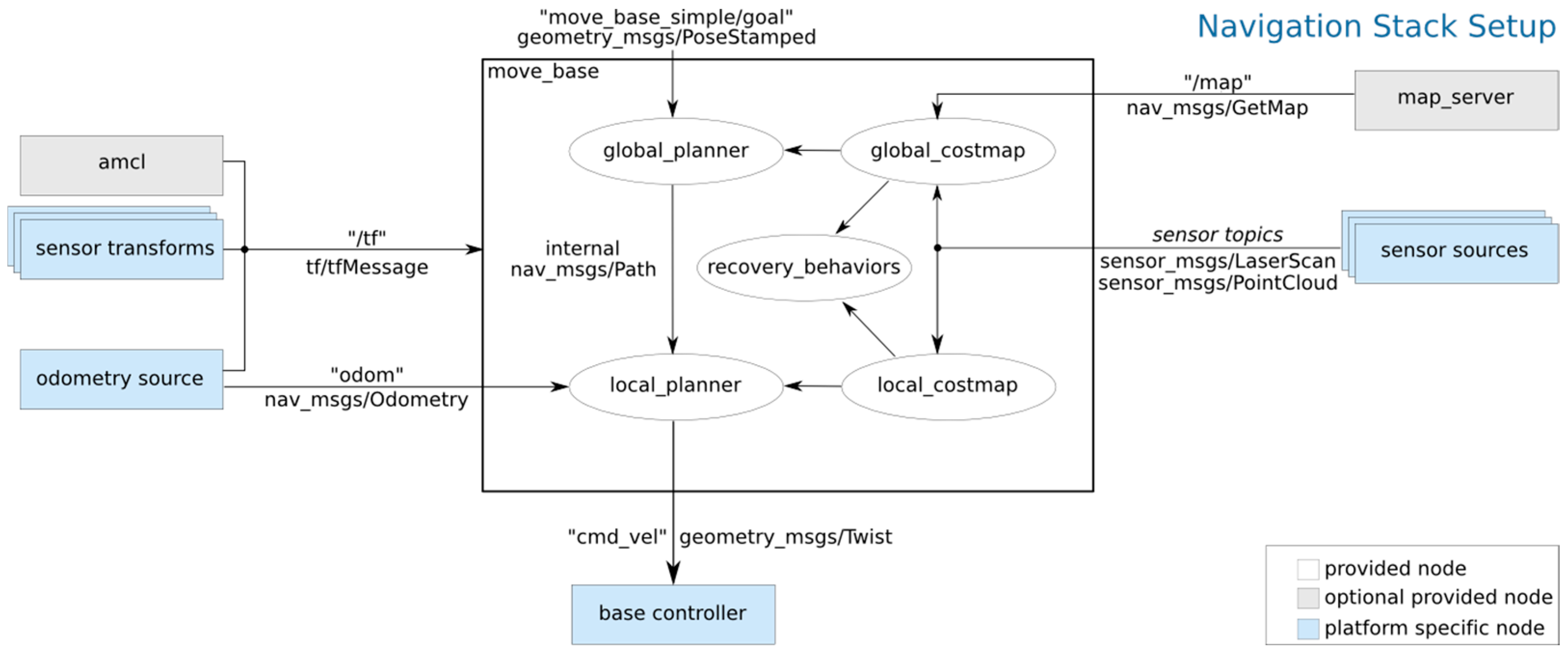
Figure 1. ROS-based autonomous navigation framework, the arrows indicate the direction of data transmission.
Information 16 00896 g001
Figure 2. 2D raster map, where green indicates the start point, red indicates the target point, and the blue dashed line represents the path, the colors represent the cost distribution of the raster map, where darker colors indicate a higher obstacle probability and lighter colors indicate a more passable area.
Information 16 00896 g002
Figure 3. Path planning algorithms with different heuristics, where green indicates the start point, red indicates the target point, and blue represents the searched nodes: (a) Dijkstra method; (b) A* method (Manhattan-inspired); (c) A* method (Euclidean inspired); (d) breadth-first search method.
Information 16 00896 g003
Figure 4. Heuristic function deviation, the direction with angle α represents the ideal heuristic direction with deviation, while the direction with angle θ represents the actual heuristic direction with deviation, the lines represent the directional relationship between the start point, the target point, and the deviation point.
Information 16 00896 g004
Figure 5. Euclidean distance heuristic function, the blue grids indicate the traversed path, while the green grids mark the key nodes involved in the heuristic computation.
Information 16 00896 g005
Figure 6. Manhattan distance heuristic function, the blue grids indicate the traversed path, while the green grids mark the key nodes involved in the heuristic computation.
Information 16 00896 g006
Figure 7. Visualization map and the corresponding real-world scene: (a) movement paths in the visualization map; (b) in real scenarios, the A* algorithm may cause the vehicle to move too close to pedestrians and obstacles.
Information 16 00896 g007
Figure 8. Schematic diagram of layered terrain (1—obstacle section, 2—gradient descent section, 3—passable section).
Information 16 00896 g008
Figure 9. Improved cost map cost principle. The curve represents the relationship between the obstacle distance d(P) and the surrogate cost value C(P) in the improved cost map. It illustrates that when the distance from the obstacle is less than the threshold R, the cost value remains high (255), and when the distance exceeds R, the cost value decreases exponentially.
Information 16 00896 g009
Figure 10. Implementation process of the method: (a) original high-precision raster map; (b) coarse-precision raster map; (c) coarse-precision raster map and passable area; (d) high-precision raster map and passable area. The letters (A–K) represent the raster nodes along the planned path and their adjacent passable areas. The white grids indicate passable regions, the black grids represent obstacles, and the blue grids denote the expanded accessible areas obtained after the two-stage A* path planning process.
Information 16 00896 g010
Figure 11. Linear interpolation effect.
Information 16 00896 g011
Figure 12. Original raster map.
Information 16 00896 g012
Figure 13. Coarse accuracy raster map.
Information 16 00896 g013
Figure 14. Improved coarse accuracy cost map.
Information 16 00896 g014
Figure 15. Coarse accuracy cost map plain path planning, the red trajectory shows the final global path.
Information 16 00896 g015
Figure 16. High-precision path planning in plain area, the red trajectory shows the final global path.
Information 16 00896 g016
Figure 17. Comparison of path planning between the original A* method and the hierarchical terrain method: (a) first path planning; (b) second path planning; (c) third path planning. The pink line represents the path planning results under different algorithms.
Information 16 00896 g017
Figure 18. Example of a real scenario of an urban industrial park: (a) ground level part of the industrial park; (b) underground parking lot.
Information 16 00896 g018
Figure 19. Vehicle travelling path and 3D mapping process. The light blue curve represents the vehicle’s actual travelling trajectory during the mapping process in the underground parking lot. The background shows the 3D point cloud data collected by the LiDAR, representing the spatial structure of the environment.
Information 16 00896 g019
Figure 20. 3D point cloud map.
Information 16 00896 g020
Figure 21. Path planning results in real scenarios. The pink line represents the planned path generated by the proposed algorithm in the real underground parking scenario, while the gray background shows the 3D LiDAR point cloud map of the environment.
Information 16 00896 g021
Figure 22. Real-time linear and angular velocities during vehicle operation.
Information 16 00896 g022
Figure 23. Dynamic obstacle avoidance of a vehicle encountering pedestrians.
Information 16 00896 g023
Figure 24. Effect of weight ratios on total running time and pedestrian avoidance speeds.
Information 16 00896 g024
Table 1. Comparison of different method runs.
Method MetricsOriginal A* MethodLayered Terrain Method
Total path length (number of rasters)523546
Proximity to obstacles (number of line segments)50
Method operation time (seconds)5.1214.091
Table 2. Comparison of local path planning methods running in different terrains.
Method Metrics (s)Layered Terrain MethodLayered Terrain + Local Path Planning Method
Corner region runtime2.5172.941
Straight ahead region runtime1.5740.476
Method computation time4.0913.417
Table 3. Comparison of local path planning methods in different terrains under real scenarios.
Method Index (s)Layered Terrain MethodLayered Terrain Method + Local Path Planning Calculation
Corner area running time6.414.73
Straight ahead region running time6.127.01
Pedestrian avoidance running time7.003.42
Method computation time19.5315.16
Table 4. Comparison of run times of different methods in various terrains.
Methods (s)Straight Ahead AreaCorner AreaCircumvention of PedestriansTotal Running Time
RRT*7.944.243.1115.29
PF-RRT*7.524.613.3815.51
A*8.273.963.1315.36
FL8.314.273.1515.73
PSO8.284.592.7115.58
CSA8.184.183.0715.43
ABC8.224.283.3118.81
ACO8.744.313.1816.23
Ours7.014.733.4215.16
Disclaimer/Publisher’s Note: The statements, opinions and data contained in all publications are solely those of the individual author(s) and contributor(s) and not of MDPI and/or the editor(s). MDPI and/or the editor(s) disclaim responsibility for any injury to people or property resulting from any ideas, methods, instructions or products referred to in the content.