Article

MoCap-Impute: A Comprehensive Benchmark and Comparative Analysis of Imputation Methods for IMU-Based Motion Capture Data

1
Peter Faber Business School, Australian Catholic University (ACU), North Sydney, NSW 2060, Australia
2
School of Electrical and Data Engineering, Faculty of Engineering and Information Technology, University of Technology Sydney (UTS), Sydney, NSW 2007, Australia
3
Department of Information Technology, College of Computing and Information Sciences, University of Technology and Applied Sciences, Ibri 511, Oman
4
Faculty of Computers and Informatics, Zagazig University, Zagazig 44519, Egypt
5
AI Applications Chair, University of Nizwa, Nizwa 616, Oman
6
Department of Data Science, Wakeb, Riyadh 13321, Saudi Arabia
7
Department of Computer Science, College of Computer Engineering and Sciences, Prince Sattam Bin Abdulaziz University, Alkharj 11942, Saudi Arabia
8
Higher Future Institute for Specialized Technological Studies, Cairo 11751, Egypt
9
Department of Computer Science, Faculty of Computers & Informatics, Suez Canal University, Ismailia 41522, Egypt
10
Department of Mathematics, Faculty of Science, Suez Canal University, Ismailia 43533, Egypt
*
Authors to whom correspondence should be addressed.
These authors contributed equally to this work.
Information 2025, 16(10), 851; https://doi.org/10.3390/info16100851
Submission received: 16 July 2025 / Revised: 10 September 2025 / Accepted: 19 September 2025 / Published: 1 October 2025
(This article belongs to the Section Information Processes)

Abstract

Motion capture (MoCap) data derived from wearable Inertial Measurement Units is essential to applications in sports science and healthcare robotics. However, a significant amount of the potential of this data is limited due to missing data derived from sensor limitations, network issues, and environmental interference. Such limitations can introduce bias, prevent the fusion of critical data streams, and ultimately compromise the integrity of human activity analysis. Despite the plethora of data imputation techniques available, there have been few systematic performance evaluations of these techniques explicitly for the time series data of IMU-derived MoCap data. We address this by evaluating the imputation performance across three distinct contexts: univariate time series, multivariate across players, and multivariate across kinematic angles. To address this limitation, we propose a systematic comparative analysis of imputation techniques, including statistical, machine learning, and deep learning techniques, in this paper. We also introduce the first publicly available MoCap dataset specifically for the purpose of benchmarking missing value imputation, with three missingness mechanisms: missing completely at random, block missingness, and a simulated value-dependent missingness pattern simulated at the signal transition points. Using data from 53 karate practitioners performing standardized movements, we artificially generated missing values to create controlled experimental conditions. We performed experiments across the 53 subjects with 39 kinematic variables, which showed that discriminating between univariate and multivariate imputation frameworks demonstrates that multivariate imputation frameworks surpassunivariate approaches when working with more complex missingness mechanisms. Specifically, multivariate approaches achieved up to a 50% error reduction (with the MAE improving from 10.8 ± 6.9 to 5.8 ± 5.5) compared to univariate methods for transition point missingness. Specialized time series deep learning models (i.e., SAITS, BRITS, GRU-D) demonstrated a superior performance with MAE values consistently below 8.0 for univariate contexts and below 3.2 for multivariate contexts across all missing data percentages, significantly surpassing traditional machine learning and statistical methods. Notable traditional methods such as Generative Adversarial Imputation Networks and Iterative Imputers exhibited a competitive performance but remained less stable than the specialized temporal models. This work offers an important baseline for future studies, in addition to recommendations for researchers looking to increase the accuracy and robustness of MoCap data analysis, as well as integrity and trustworthiness.

1. Introduction

MoCap has become a critical aspect of studying various human activities in sports science [1,2] and in studying human disorders in neurosciences [3]. This includes capturing gestures using Inertial Measurement Unit (IMU) sensors to study various human movements. IMU wearable sensors are used to capture players’ sport skills for further study and analysis, such as human performance assessment [4,5,6,7].
IMU sensors have recently gained popularity due to their widespread use in wearable devices that aid in the detection of body part motion and orientation. They have the ability to offer acceptable data rates and provide digital outputs, together with their reasonable cost and extended lifetime. Several applications of IMUs have been found, including capturing and monitoring the movement of athletes in order to assess their talent and document their professional motion [8]. In addition, they have been used for healthcare challenges, such as neurological illnesses, where they are employed in daily activities and environments for remote diagnosis and rehabilitation direction [9]. Additional uses include professional motion capture studios and intensive 3D animation and design resources [10]. During the collection of digital data, however, some data may be lost due to the battery life of the sensors or inadequate network connectivity. Likewise, the presence of metallic items in the surroundings of IMUs might impact the accuracy of the collected data.
To our knowledge, despite the benefits of IMU sensors to a wide range of applications, imputation of the data obtained from IMU sensors remains underexplored. The IMU sensors’ readings are impacted negatively by several factors, including drifting, the placement of the sensors, and magnetic field interference [11]. These issues result in missing data, which may lead to corrupted data, inaccurate outcomes, or biased results. Data imputation is therefore required early in the preprocessing stage to treat missing data. This study investigates the effectiveness of typical data imputation techniques when applied to MoCap data gained from IMU wearable sensors. However, the comprehensive performance of imputation techniques specifically for this type of sensory data remains underexplored in the existing literature. As a consequence, this study provides the first MoCap-based dataset for benchmarking various data imputation methods and then reports on the performance of the data imputation techniques. The issue of missing data is evaluated for MoCap data. The models utilized in this study belong to three major categories, namely machine learning (ML), deep learning (DL), and statistical methods. The key contributions of this study are generating a new dataset from a publicly available MoCap dataset [2] gathered using IMU wearable sensors to be utilized to impute the missing values and addressing the state-of-the-art imputation methods. To our knowledge, this is the first dataset to be introduced into the field.
To provide readers with a clear overview of our research design, Figure 1 depicts the overall MoCap data imputation methodology employed in this study. The detailed methodology is explained in Section 3.
The remainder of this paper is structured as follows. In Section 2, related works with the missing data imputation methods are addressed. The proposed dataset along with the proposed methodology and data evaluation metrics are presented in Section 3. Section 4 lists and discusses the study results. Finally, this paper is concluded in Section 5.

2. Background and Related Work

2.1. IMUs

IMU sensors have achieved popularity in recent years in numerous applications, including manufacturing, robotics, and healthcare evaluations [12]. IMUs are portable electronic equipment used to track and measure angular velocity and body motion. Different forms of data collection sensors exist, such as accelerometers, gyroscopes, and magnetometers. Accelerometers and gyroscopes measure the inertial acceleration and rotational angle. However, a magnetometer measures the bearing magnetic direction, which enhances the acquired readings and means that it is considered an advanced sort of sensor. IMUs are considered some of the most straightforward and rapid means of capturing the motion of body parts due to the omission of cable extensions during data acquisition [13,14,15]. As IMUs have been extensively applied to determining motion in terms of acceleration, angular velocity, and orientation [16], an accelerometer measures the total acceleration a m as shown in Equation (1).
a m = a b + g + η a
where a b represents the body’s acceleration due to external forces, g represents the gravitational acceleration vector with a magnitude of 9.81 m/s2, and  η a represents accelerometer noise.
The angular velocity ω m is quantified in degrees per second using the gyroscope sensor:
ω m = ω t + b g + η g
where ω t is the actual angular velocity, b g is the gyroscope bias, and  η g is the gyroscope noise.
The relationship between orientation θ orintation ( t ) and actual angular velocity is ω t ( t ) = d θ orintation ( t ) / d t . In discrete time, orientation is estimated by integrating measured angular velocity using the Euler integration:
θ orintation ( t ) θ orintation ( t Δ t ) + ω m ( t Δ t ) · Δ t
where Δ t is the sampling interval.
Unfortunately, accuracy cannot be guaranteed when depending on an accelerometer and gyroscope because of the presence of noise and the gyroscope drift. Thus, a magnetometer is incorporated to determine the yaw angle rotation which improves the gyroscope drift. However, readings from the magnetometer sensor can be affected by surrounding metals or electronic objects [16]. Using IMUs, the data for calibration is collected only in the gravitational field so that the calculated scale factor of each axis is limited to the range of [−1 g, 1 g]. Such limitation prevents tasks with large gravity values [17,18]. However, this limitation has been overcome by rotating the accelerometer sensor around a given point to detect centripetal and Euler acceleration. Consequently, the detection range of the accelerometer sensor has been expanded [19,20,21,22,23]. These limitations of the IMU sensors are a direct explanation of some of the missingness mechanisms examined in this study. The presence of noise, gyroscope drift, and magnetic disturbances introduces instability in sensor readings, which consequently yields gaps in measurements or periods of missing data. In addition, calibration restrictions and range restrictions may yield sequences where motion capture is not possible and may produce block-missing sequences. Consequently, the physical limitations of IMU sensors explain the prevalence of missing data in motion capture studies and underscore the need to develop robust imputation models.

2.2. Data Imputation

Recent progress in ML has produced very robust strategies for addressing missing data in time series. There are methods that can employ deep learning to model complex data distributions and provide estimators employing robust features of imputation. For instance, conditional score-based diffusion models (CSDIs) have become a promising alternative to traditional probabilistic time series imputation, creating a greater level of performance by providing multiple plausible imputed values denoted from the uncertainty of the missing values rather than an independent point estimate [24]. This is especially important to sports science because sensor data captured with wearables (e.g., IMUs) may be missing due to failure of the sensor, human error, or other technical issues. Analyzing datasets is critical since they are considered a rich source of information for different types of knowledge. Nevertheless, missing data in these datasets can prevent the generation of complete information, which is necessary to make a wise intelligent decision [25]. Hence, the issues that arise when data are missing can introduce bias and lack of recoverability. For this reason, several studies have been conducted on missing data imputation to impute missing data [25,26,27,28]. Data imputation techniques are designed to substitute any missing data samples by randomly estimating data from the same datasets. The data can undergo single or multiple imputation. In single imputation, only one estimate is used, whereas various estimates are used in multiple imputation. The missing data can be categorized as (1) missing completely at random, (2) missing at random, or (3) missing not at random [29,30].
Data missing completely at random occurs when parts of the data collected are missing by design due to out-of-hand circumstances (i.e., unobserved data). In other words, missingness occurs during the data acquisition process and thus becomes of no interest. Hence, there is no correlation between the observed and missing data. A popular example is data being missed while using IMUs due to sensor failure or network connection problems. In this case, there is no bias to be introduced, and data is estimated from the observed original data on average. The standard estimates errors are usually substantial due to the reduced sample size [31,32,33,34]. Missing data becomes missing at random if the information is missing from the observed data after confirming the dataset. Thus, a correlation exists between the observed and missing data [25].
In both cases, multiple imputation is utilized to replace the missing data with appropriate predictive data. The principle behind multiple imputation is to predict the missing values using the observed dataset. The imputed values are estimated rather than known or uncertain; this process is repeated several times to create several complete datasets. The analysis model is then fitted to each generated dataset, and the results are combined for inference using Rubin’s MI rules [32,35]. However, this estimation remains inefficient enough, as the data still incomplete. The third technique is used when valuable information is lost from the dataset and there is no universal method to handle the missing data properly. Thus, the missing data depends on its value. Hence, missing data is missing not at random when it is not classified as missing at random or missing completely at random [26,30].

2.3. Single Imputation Methods

Single imputation (SI) techniques are used in handling missing data in research by replacing the missing data with a single value. This includes implementing Mean Imputation [36], Last Observation Carried Forward (LOCF) [37], Regression Imputation [38], Hot Deck Imputation [39], Forward Imputation [40], Single Ratio Imputation [41], Median Imputation [42], and K-Nearest Neighbors (KNN) imputation [43].
SI approaches are effective in handling missing data across various sports science scenarios. Team Mean Imputation is used to impute workload data in youth basketball [44]. The average workload of the team for the specific session is used to impute missing workload data including jumps per hour and RPE for high-school basketball players. However, this approach cannot always be calculated, may not account for individual variations, and could introduce bias if team performance varies significantly. KNN imputation is employed to predict missing split times for runners who did not finish the Boston Marathon [45]. Local regression based on KNN is used to estimate missing times. However, performance depends on the choice of neighbors and may not generalize well to different datasets. Last Observation Carried Forward (LOCF) is used in [46] to monitor Total Quality Recovery (TQR) scores and race performance for college swimmers over two seasons. The missing TQR score is imputed with the TQR score recorded for that same participant on the preceding day. Although LOCF is generally a less sophisticated imputation approach, it unrealistically assumes that a variable remains constant over the period where data is missing. Therefore, LOCF is incapable of capturing daily fluctuations in an athlete’s recovery status.
In addition, when model-based imputation methods are inappropriate, due to limitations present in the data, single-imputation procedures, such as random Hot Deck Imputation, may serve as an alternative. Random Hot Deck Imputation is a valuable procedure because it yields plausible imputed values through matching records that contain missing data to records with complete observations; thus, it does not arbitrarily alter the dataset [39]. SI procedures can also be valuable for analyzing changes in outcome variables such as behaviors, performance, and psychological constructs. They are beneficial for preserving survey continuity when evaluating intended changes resulting from interventions [47]. Single imputation can be a simple way to impute missing values when gaps are short or missing source assignment lengths are very short [48]. Finally, Forward Imputation and missForest can potentially also yield robust imputation results across commonly encountered data patterns, both of which exhibit varying degrees of excess kurtosis, skewness, and correlated structures. Forward Imputation and missForest are useful when timely and appropriate imputation is required, without strong distributional assumptions [40].
Although SI techniques are often used to handle missing data, there are several important issues related to validity and reliability with the use of SI. SI techniques will replace each missing value with a single value. When replacing a missing value with a single, fixed value, SI techniques do not take into account the imputation uncertainty with missing data. They risk causing an under-estimation of standard errors, thus leading to confidence intervals that are overly narrow, which may result in an increased rate of false positives [29]. Replacing a missing value with a single value can also affect the relationships that exist; it can distort the correlational relationships that we are investigating, as well as the coefficients we are testing. For example, it is known that Mean Imputation typically reduces correlations. This is challenging within sports science where understanding the relationships between performance metrics, training loads physiological responses. The validity of single imputation methods will depend upon the imputation methods chosen. Multiple different SI methods can produce very different results and thus impact the reliability and consistency of the findings, leading to biased imputations [44]. Mean imputation can distort the distribution of the data.
Moreover, data in sports science can be markedly variable and context-specific, and single imputation methods may not work well with complex data structures. This can lead to implausible imputed values and further bias [39]. Single imputation methods are also less effective when data are not missing completely at random (MCAR). They do not perform well under missing at random (MAR) or missing not at random (MNAR) conditions, which are common in sports science data. Methods including Mean, Median, or Mode Imputation often do not adequately address the underlying mechanisms that cause the data to be missing, leading to biased estimates and incorrect conclusions [48,49,50,51]. Single imputation is also limited in longitudinal sports science-related studies. This because it can lead to biased estimates of trends and associations over time, where tracking changes in performance or health metrics over time is crucial [44]. For instance, it does not adequately handle the correlation between repeated measures, which can distort the analysis of longitudinal data [37].

2.4. Multiple Imputation Methods

Multiple imputation (MI) is an a statistical technique used to handle missing data. MI produces multiple datasets with imputed missing data, analyzes each one separately, and combines the results to represent uncertainty due to missing data [52]. The primary strength of MI over SI methods is that MI estimates the parameters with fewer limits of bias and more accurately derives variance estimates and confidence intervals [53]. Methods for using MI that have been seen in sport science include chained equations [53], joint models [54], Markov chain bootstrapping [55], Monotone Imputation [56], and random Hot Deck Imputation [39].
MI methods are already regularly and commonly used in sport science. A recent example of MI can be seen in the recent article evaluating the monitoring of athlete workloads [44] for longitudinal studies that monitor athlete workload. The authors proposed to impute workload for youth basketball players based on the workload variable of jumps per hour using regression-based methods in MI that use numerous predictors. The authors used MI only to impute the workload variables and did not include any other non-workload data that might have improved their imputations’ quality. In sport injury epidemiology, a predictive model-based MI was used to estimate missing weekly game hours for 2098 youth ice hockey players [36]. The imputed estimates represent the mean hour estimates from the imputed samples. The statistical models used for their data included Poisson, zero-inflated Poisson, and negative binomial regressions, which were utilized on the imputed datasets to estimate injury rate ratios. In [36] they found that when the dataset had few to moderate proportional missing data for weekly game hours, MI had a similar performance to mean imputation.
A new MI method for auto-correlated multivariate count data from accelerometers was developed in [57]. It uses mixture of zero-inflated Poisson and Log-normal to handle characteristics including autocorrelation and over/under-dispersion of count data. However, the characteristics of accelerometer data, such as autocorrelated multivariate counts, still create challenges in imputation. A framework for multilevel data was proposed in [58] to estimate aging curves for offensive players in Major League Baseball (MLB). This study treats unobserved seasons due to player dropouts as missing data. Player performance metrics associated with missing seasons are imputed, and aging curves are then constructed using these imputed datasets. The main limitation is accurately modeling the reasons for player dropout and the performance trajectories of those who drop out. Another study represents a direct comparison of multiple imputation to alternative methods of addressing missing data in the context of Rugby [59]. The research focuses on the sports-specific variable of the rate of perceived exertion (RPE) that is routinely missing from large datasets.
Despite the merits of using MI over SI, MI has several limitations. MI typically performs best under MCAR or MAR assumptions. If data are MNAR, standard MI may produce biased results unless the MNAR mechanism is explicitly modeled or sensitivity analyses are conducted [60]. Moreover, implementing MI methods correctly requires statistical knowledge and familiarity with relevant software [44]. The accuracy of MI methods is also challenging due to its heavy reliance on the correct specification of the imputation model. This includes choosing the right variables to include in the model and specifying the appropriate relationships [61]. Another limitation is that MI methods can be computationally intensive for large datasets with many variables and complex patterns of missingness [60]. However, modern software and multi-core processors have alleviated this to some extent.

2.5. Gap Analysis

MoCap systems utilizing IMUs have become essential as important analysis tools for studying human activities and sports across multiple fields: sports science, human performance assessment, the diagnostic properties of certain neurodegenerative disorders, and 3D animation [1,3]. MoCap systems have high utility for human activity analysis; however, there are multiple potential sources of error in the IMU sensor data when using these systems, such as battery limitations, network issues, magnetic fields, drift and placement variability, which can cause missing data (i.e., missing time series data) [11]. It is critical that any lost or missing data are addressed to eliminate bias and inaccurate information that impede data reliability for subsequent analyses and decision making to assess how various data sources interface. Therefore, effective and appropriate data imputation methodologies should be explored and applied for use in MoCap analysis. The literature supports many data imputation methods but concentrates on SI and MI methodologies, as well as some basic statistical or non-statistical methodologies. However, it only discusses SI or MI methodologies in relation to sports science broadly, thus presenting a notable gap in the literature for the classification and evaluation of data imputation methodologies specific to MoCap data and IMU wearable sensors in order to enhance the capabilities of MoCap [11]. Entirely separate from MoCap data, data imputation studies focus on other types of data with variability in missing data mechanisms and contexts that are not reflective of continuous time series data or the nature of the missing time series data (e.g., sequential, biomechanical constraints). In our review of the literature, we identified a couple of important gaps that this study addresses. detailed as follows.
  • Lack of comprehensive performance evaluation for IMU-based MoCap imputation: To date, no research has systematically examined and compared the performance of well-established data imputation strategies, including ML and DL statistical methods, specifically for MoCap data acquired from IMU sensors. This absence limits the ability of researchers and practitioners to select the most appropriate imputation technique for specific MoCap missing data scenarios, hindering accurate data reconstruction and subsequent analysis.
  • Absence of a standardized MoCap benchmark dataset for imputation: A fundamental requirement for reproducible research and comparative analysis is the availability of a standardized dataset. Currently, there is no publicly available MoCap dataset explicitly designed and proposed for benchmarking the performance of various data imputation methods. This hinders the consistent evaluation and advancement of imputation techniques tailored to the unique complexities of MoCap data.
This research directly addresses these important gaps by providing the first thorough performance comparison of major data imputation methods in the context of ML, DL, and statistical methods as they relate to IMU-based MoCap data. As a result of this comparison, we offer definitive recommendations of the best techniques for specific cases of incomplete MoCap data. Furthermore, we introduce the first dedicated MoCap dataset as a benchmark for research focused on missing value imputation in order to stimulate future research and ensure that there is a consistent method of benchmarking in use in the community. By addressing these gaps, this work contributes to theories of data processing and advances the state of the art of robust information fusion from IMU-based motion data. We also offer practical, official recommendations for best practices in enhancing data quality and use.

3. Methodology

This section details the experimental methods used to test different data imputation methods on a multivariate time series dataset comprising simulated human motion data. We describe the dataset’s structure, the methodology for simulating missing data under a variety of mechanisms, the imputation framework including which specific algorithms were tested, and the measures used to evaluate the performance of the imputation algorithms.

3.1. Overview

The proposed methodology for evaluating the MoCap data imputation is illustrated in Figure 1. To emulate real-world scenarios, the procedure begins with the entry of MoCap data with purposefully absent values. To prepare the raw data for the subsequent imputation phase, it undergoes cleaning, normalization, and standardization.
Once the data has been preprocessed, it is directed to the basis of our system: a suite of imputation algorithms. This suite contains a variety of methods, including ML strategies such as Bsi-ML, Iterative Imputer-ML KNN-ML, the DL method DL-based Generative Adversarial Imputation Network (DL-GAIN), as well as statistical methods such as Simplefill mean and Simplefill median. By employing a variety of techniques, our proposed study aims to accommodate the diverse details and complexities inherent in MoCap data, thereby guaranteeing optimal data imputation.
The processed data are subjected to a strict evaluation after imputation. This phase of evaluation assesses the effectiveness of the selected imputation algorithms by comparing the imputed values to the original data. Metric calculation, including the critical Mean Absolute Error (MAE), is employed to further refine the evaluation. These metrics quantify the accuracy and dependability of the imputed data, demonstrating the model’s proficiency.
Following a robust evaluation and calculation of metrics, the system produces the imputed dataset. This dataset, augmented by the systematic processes of our methodology, not only represents the missing MoCap data but also demonstrates the convergence of ML, DL statistical techniques in addressing the challenges posed by missing data. Our proposed system offers an effective solution for MoCap data imputation with this integrated approach.

3.2. Dataset and Preprocessing

Due to the nature of our study, we utilized a multivariate time series dataset with P distinct persons (players) who are performing a specific skill which is publicly available [2]. This dataset includes four standardized karate skills performed by top members of the Egyptian men’s national team, namely, (1) Gedan Barai (downward block: an upper-body–centered, linear defensive motion), (2) Oi-zuki (lunge punch: a linear forward offensive strike involving both trunk and arm), (3) Jodan Age–uke (upper block against head attacks: an upward defensive motion with rotation) and (4) Soto–uke (outside inward block: a rotational defensive arm movement). These karate skills are considered fundamental techniques of karate and span different kinematic characteristics. In this dataset, each player has data collected for T discrete time points and A features that correspond to measured IMU sensor readings. The original complete dataset is stored as a tensor X R P × T × A . For the experiments we describe in this paper, we have a dataset with dimensions P = 53 , T = 100   A = 39 . While this dataset does not suffer from missing values, we propose using it to artificially include missing values with three different mechanisms.
We propose a preprocessing step for the original dataset, which is normalization. The dataset undergoes mi-n-max normalization prior to the use of some of the imputation methods, specifically those that are particularly sensitive to feature scaling, such as neural network-based methods like GAIN. For each feature a (angle), we scale the time series X : , : , a across all players and time points to the range [0, 1], using the following formula:
X norm , p , t , a = X p , t , a min p , t ( X p , t , a ) max p , t ( X p , t , a ) min p , t ( X p , t , a ) + ϵ
where the m i n and m a x are calculated over the observed entries only for that feature a. ϵ is a small constant (e.g., 10 6 ) for numerical stability  p , p and t   t are dummy indices that range over all players and time points, respectively. We take the parameters min ( · ) and max ( · ) for each feature and save them in order to perform an inverse transformation (renormalization) back to the original scale of the data post imputation so that we can estimate the meaningful error.
The dataset used in this study is based on a publicly available dataset [2]. The original dataset describes IMU data collected from 53 elite adult male participants from the Egyptian national karate team (who participate at the international-level) performing four standardized skills. No further demographic characteristics (age range, size, rank, or history of training) were detailed in the original published dataset [2]. Researchers should consider the homogeneity of this elite cohort in their assessment of generalizability. The primary contribution of this work is the generation of new benchmark datasets by introducing controlled missing values under different mechanisms and comparison of the performance of existing imputation methods.
Of note, due to limitations on space and the total number of visualizations, all reported experiments in Section 4.1 and Section 4.2 were conducted using the Gedan Barai (downward block) subset of the dataset. The additional three standardized skills (i.e., Oi-zuki, Jodan Age-uke and Soto-uke) are included in the original dataset and available for use. This decision was made to enable more detailed reporting of methods within the length constraints of the manuscript. However, the full benchmark dataset can be used to replicate and build upon the work described here.

3.3. Simulation of Missing Data

Missing values were artificially generated within the complete dataset X to create controlled experimental conditions for assessing imputation performance. This process produces a missing data tensor X miss  and then a corresponding binary mask tensor M { 0 , 1 } P × T × A . The symbol M p , t , a = 1 indicates the value X p , t , a is missing (NaN in X miss ), while M p , t , a = 0 signifies that the value is observed.
The missing data entries were independently generated for each univariate time series X p , : , a based on a specified number of missingness count k, corresponding to a fraction k / T of the total series length (which ranged between 5% and 30% in our experiments)  according to one of three different missing data mechanisms, denoted by ζ .
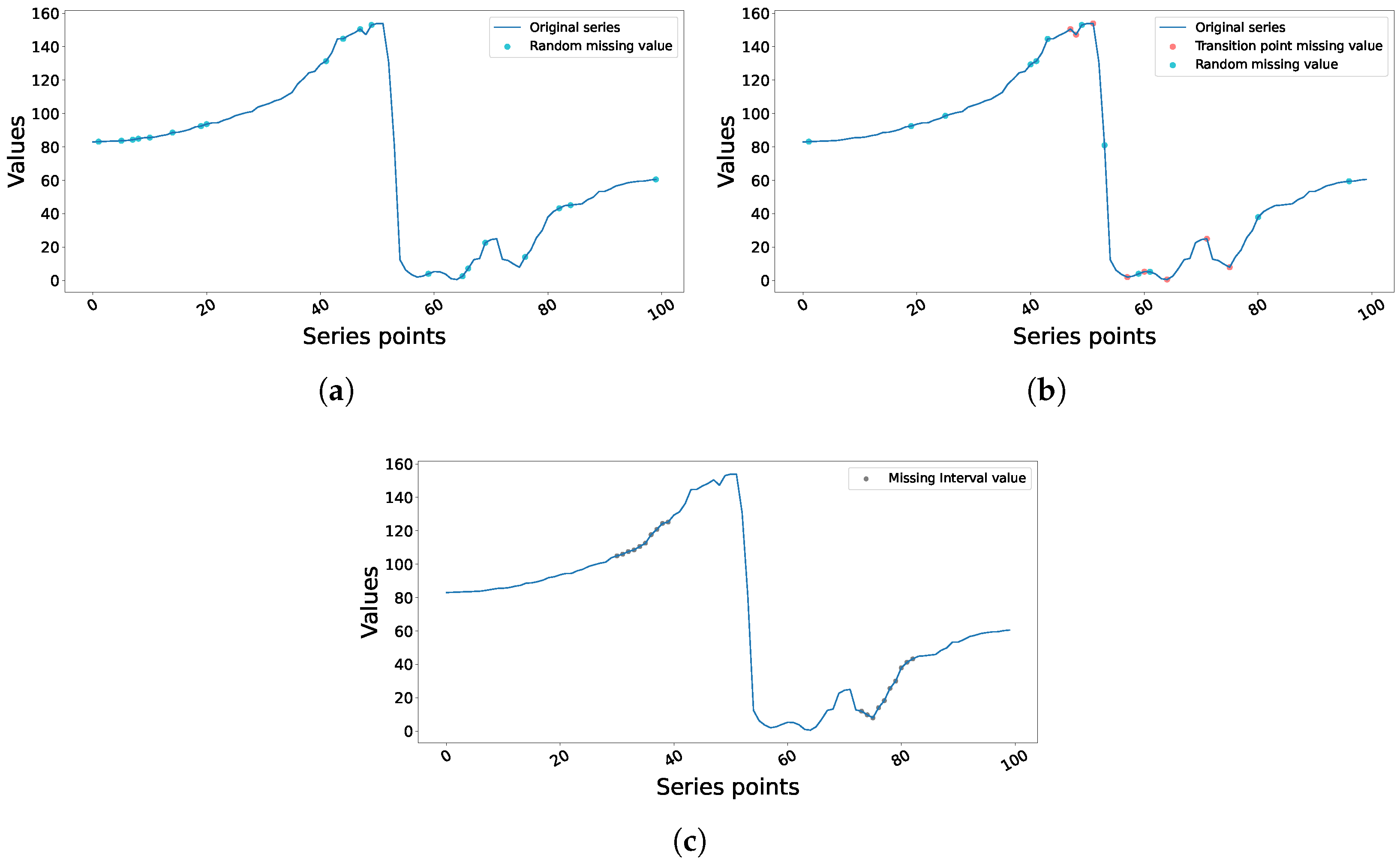
  • Missing Completely At Random (MCAR): From { 0 , 1 , , T 1 } , k unique time indices were sampled uniformly without replacement for each series X p , : , a , and the corresponding entries in M p , : , a were assigned a value of 1. This mechanism assumes that missingness was completely independent of observed and unobserved values. A sample of this approach is depicted in Figure 2a.
  • Value-Dependent Missingness at Transition Points: This mechanism emulates a form of value-dependent missingness, where the probability of data loss is intentionally correlated with the local dynamics of the signal itself. Specifically, we target transition points (local minima and maxima), as these points of high kinetic change can be more susceptible to measurement error or signal clipping in real-world MoCap applications. First, for each time series X p , : , a , we identify the complete set of transition point indices T p , a . Then, we randomly sample k = min ( k , | T p , a | ) indices from these transition points. If the total number of missing points to be introduced, k, is greater than the number of available transition points, we sample the remaining k k indices from the non-transition points. All sampled indices were set to missing ( M p , t , a = 1 ). Figure 2b shows a sample of this approach.
  • Block Missingness (Structured): We introduced blocks of contiguous missing values. For the purposes of sampling blocks, the total length of the time series T was conceptually divided into segments of N b . For each segment, we placed a block of a predetermined size L b (where L b was identified to approximate the total count of k across all blocks) starting from a random index within the limits of the segment. Again, all sample indices in these N b blocks were converted to missing in M . In the case of overlaps in blocks or deviations in total segment length which deemed the total count < k (or >k), we made adjustments. Figure 2c depicts a sample of this dataset.
The missing data mask M was generated according to these mechanisms as formalized in Algorithm 1. The algorithm iterates through each player p and angle a and applies the missingness mechanism ζ to the corresponding indexed time series to identify the set of indices ‘idx’ to undergo masking updates the mask tensor M, specifying which mechanism’s logic was used for each mechanism (MCAR, Transition, Block) in the specified conditional statements.
Algorithm 1 GenerateMissingMask ( X , k , mechanism )
Require: 
Complete data tensor X R P × T × A , Missing count k, ζ mechanism
Ensure: 
Mask tensor M { 0 , 1 } P × T × A
   1:
Initialize M 0 P × T × A
   2:
for  p { 1 , , P }   do
   3:
    for  a { 1 , , A }  do
   4:
        Let S X p , : , a be the time series
   5:
        Let I m i s s be the set of indices to mask
   6:
        if  mechanism = MCAR  then
   7:
            I m i s s RandomSample ( { 1 , , T } , k )
   8:
        else if  mechanism = Transition  then
   9:
            I t r a n s FindLocalExtremaIndices ( S )
  10:
            I s a m p l e RandomSample ( I t r a n s , min ( k , | I t r a n s | ) )
  11:
           if  | I s a m p l e | < k  then
  12:
                I r e m a i n { 1 , , T } I t r a n s
  13:
                I s a m p l e I s a m p l e RandomSample ( I r e m a i n , k | I s a m p l e | )
  14:
           end if
  15:
            I m i s s I s a m p l e
  16:
        else if  mechanism = Block  then
  17:
           Let N b , L b be block parameters s.t. N b · L b k
  18:
           Partition { 1 , , T } into N b segments, S e g 1 , , S e g N b
  19:
           for  i { 1 , , N b }  do
  20:
                s t a r t _ i d x RandomInt ( min ( S e g i ) , max ( S e g i ) L b )
  21:
                I m i s s I m i s s { s t a r t _ i d x , , s t a r t _ i d x + L b 1 }
  22:
           end for
  23:
           Trim or extend I m i s s to ensure | I m i s s | = k
  24:
        end if
  25:
         M p , I m i s s , a 1
  26:
    end for
  27:
end for
  28:
return M

3.4. Imputation Framework Contexts

To clarify on how different imputation methods can take advantage of the structure in the dataset, we applied algorithms in three different information contexts as follows.
  • Univariate Context: Here, data are processed independently for each individual time series X p , : , a R T . Univariate algorithms will only learn from information in the individual series being completed; a limitation of univariate context is that we ignore any potential relationships across players or angles. Input data is treated as a vector with length T.
  • Multivariate Context (Across Players): For a given angle a, we conceptualize imputation as the data matrix X : , : , a R P × T (or the transpose). As a result, algorithms that in the multivariate context can model correlations or similarities across different players and time series across angles will take advantage of information from the cohort.
  • Multivariate Context (Across Angles): For a given player p, we represent imputation as the data matrix X p , : , : R T × A . Algorithms that operate in the multivariate context can take advantage of inter-feature correlations, essentially learning about how various angles (kinematic variables) are related to the same subject over time.
This exploration of a potentially varied context facilitates a more precise evaluation of the advantages either gained or lost by utilizing information across players or angles compared to univariate means.

3.5. Imputation Algorithms

We implemented and compared a diverse set of imputation algorithms, spanning statistical baselines to state-of-the-art deep learning models.
  • Statistical Baselines: Simple, computationally economical methods including Mean, Median, and Random Sample Imputation applied within the relevant context (univariate series or multivariate scope across players/angles for calculating the statistic or sampling pool).
  • Classical Machine Learning Methods: Algorithms primarily sourced from the fancyimpute library.
    KNN estimates missing values using a weighted average of the values from the K most similar samples (neighbors), based on observed features.
    Matrix Factorization (SoftImpute, IterativeSVD): These methods approximate the data matrix with a low-rank factorization, effectively filling missing entries based on learned latent factors. SoftImpute uses nuclear norm regularization, while IterativeSVD employs truncated SVD iteratively.
    IterativeImputer models each feature with missing values as a function of the other features using a regression model (e.g., Bayesian Ridge). It iteratively predicts and updates missing values until convergence.
    Optimal Transport Imputation (OT) [62]: This method utilizes Optimal Transport theory, specifically minimizing the Sinkhorn divergence S ϵ ( · , · ) between empirical distributions formed by batches of data. We utilize the BatchSinkhornImputation approach, where the missing values themselves are treated as learnable parameters θ . In the following text, we will call this method BSI. These parameters are optimized by minimizing the expected Sinkhorn divergence between pairs of randomly drawn mini-batches ( B 1 , B 2 ) from the currently filled dataset X filled ( θ ) :
    min θ L OT = E ( B 1 , B 2 ) [ S ϵ ( X filled ( θ ) [ B 1 ] , X filled ( θ ) [ B 2 ] ) ]
    The expectation is approximated using N pairs samples per gradient step.
  • Deep Learning Methods:
    SAITS [63]: Self-Attention-based Imputation for Time Series (SAITS) is a deep learning model that can impute missing data from complex time series data. SAITS addresses an important challenge of many previous imputation models, which is the lack of a self-attention-based mechanism to capture long-range dependencies detectable within the time series data [63]. Capturing these long-term relationships is particularly important when attempting to impute values in irregularly sampled time series and/or partially observed time series.
    BRITS [64]: BRITS is a novel technique that uses bidirectional recurrent neural networks (RNNs) to impute missing values in multivariate time series data. Unlike earlier techniques, BRITS makes no particular data assumptions and learns missing values directly within a recurrent dynamical system. It enables efficient backpropagation updates by treating missing values as variables in the RNN graph. The model increases overall accuracy by carrying out imputation and classification/regression at the same time. This method tackles issues such as nonlinear dynamics in time series and correlated missing values.
    GRU-D [65] is proposed specifically for multivariate time series with missing values, with an emphasis on “informative missingness.” It employs a Gated Recurrent Unit (GRU) architecture and integrates time interval and masking as two representations of missing patterns. GRU-D successfully captures long-term temporal dependencies and employs missingness for better prediction by incorporating these patterns into the inputs and hidden states of the GRU through trainable decay mechanisms. This method improves classification performance on synthetic and real-world clinical datasets.
    CSDI [24]: The CSDI (Conditional Score-based Diffusion Model) is a deep generative approach for probabilistic time series imputation. To deal with missing values, it makes use of score-based diffusion models, which use iterative denoising to learn data distributions. CSDI produces diverse and realistic imputations by conditioning the diffusion process on observed portions of the time series. It is appropriate for probabilistic forecasting since it offers imputations and uncertainty estimates.
    GAIN [66]: GAIN utilizes a minimax game between a Generator (G) and a Discriminator (D). The Generator (G) attempts to impute the missing values in the data tensor X miss given a mask M and a noise tensor Z, producing the final imputed tensor X ^ = X miss ( 1 M ) + G ( X miss , M , Z ) M . The discriminator D attempts to differentiate observed components from imputed ones based on X ^ and a hint vector H (partially revealing M ). The objectives are
    min D L D = E X , M , H [ M log D ( X ^ , H ) + ( 1 M ) log ( 1 D ( X ^ , H ) ) ]
    min G L G = E X , M , H [ log ( D ( X ^ , H ) ) ] + α E X , M [ M ( X G ( X , M , Z ) ) 2 2 ]
    where ⊙ denotes element-wise multiplication and α is a hyperparameter balancing the adversarial loss and a direct reconstruction (MSE) loss on observed components.

3.6. Evaluation Metrics

To quantitatively assess imputation accuracy, values X ^ p , t , a were compared to their respective known ground truth values X p , t , a only at the locations where the data had been artificially made missing (i.e., M p , t , a = 1 ). The primary measure of performance for our study was the Mean Absolute Error (MAE), used to quantify the average size of the imputation:
MAE = p , t , a M p , t , a · | X p , t , a X ^ p , t , a | p , t , a M p , t , a
We also calculated the standard deviation of the absolute errors, STD ( { | X p , t , a X ^ p , t , a | M p , t , a = 1 } ) , which serves as a measure of variability or consistency across errors resulting from a particular method. The metrics were pooled and reported out based on the experiment context (e.g., across a whole context as an average across missing points, or per player/angle).

3.7. Experimental Setup and Implementation

The entire experimental procedure utilized essential libraries such as NumPy 2.3.0 (for numerical tasks), Pandas 2.3.2 (for handling data), Scikit-learn 1.4.2 (for baseline ML models), TensorFlow 2.18 (for GAIN), PyTorch 2.7.0, GeomLoss 0.2.6 (for OT imputation), and FancyImpute 0.7.0 (for many classical methods). Due to the extensive scope of the experiments (e.g., multiple combinations of parameters: skills, missingness levels, mechanisms, imputation contexts algorithms), computational time was critically important. We used Python 3.11’s multiprocessing library to run imputation tasks simultaneously across different CPU cores. This allowed us to assign independent imputation tasks (e.g., different series or matrices based on context) to different processes. We used shared memory arrays (multiprocessing.Array), built into helper functions to provide process-safe access, to accumulate results from concurrent processes.
An overview of the whole experimental procedure, which included data generation, imputation, and evaluation of different configurations, is presented conceptually in Algorithm 2. Algorithm 2 iterates through each of the experimental configurations; it loads/generates the data and the mask, applies the algorithm within the context, performs calculations of performance, and stores the result. The ‘ApplyImputation’ step presents a conceptual definition of executing the chosen algorithm, including any intended data slicing based on the context and possible parallelized operation.
Algorithm 2 Experimental Configuration
Require: 
Dataset X, Players P, time series length T, Features A
   1:
Define Imputation Methods F { GAIN , IterativeImputer , KNN , }
   2:
Define Missingness Mechanisms ζ { MCAR , Transition , Block }
   3:
Define Missingness Proportions K { 0.05 , 0.10 , 0.15 , 0.20 , 0.25 , 0.30 }
   4:
Define Imputation Contexts C { Univariate , Multivariate Player , Multivariate Angle }
   5:
Initialize Results storage R e s u l t s
   6:
for all  f F   do
   7:
    for all  m ζ  do
   8:
        for all  i K  do
   9:
           Let k i · T
  10:
          Generate Mask M GenerateMissingMask ( X , k , m )
  11:
          for all  c C  do
  12:
                X ^ ApplyImputation ( X , M , f , c )
  13:
                M A E CalculateMAE ( X , X ^ , M )
  14:
                S t d E r r CalculateStdErr ( X , X ^ , M )
  15:
                R e s u l t s R e s u l t s { ( f , m , i , c ) : ( M A E , S t d E r r ) }
  16:
           end for
  17:
        end for
  18:
    end for
  19:
end for
  20:
return   R e s u l t s
To formalize the fundamental imputation process across the experimental conditions, we present Algorithm 3, which proposes context-aware imputation methods. Algorithm 3 is a dispatcher that arranges the data before passing it to an imputation function f. It essentially first copies the working data to a working dataset, denoted X m i s s , which presents the data with missing values represented as N a N . Next, it systematically slices the data tensor based on the specified context c. In the case of Univariate, the data are iterated through in an individual time series manner, whereas the multivariate player and multivariate angle formats create two-dimensional data matrices containing all the data by angle (all players) or by player (all angles), respectively. This structured context-aware approach enables each of the imputation methods to be applied to the data so that each method can take advantage of the different correlations between temporal data, players, or features that define the context in which they are being applied.
Algorithm 3 ApplyImputation( X , M , method , context )
Require: 
Data X, Mask M, Imputation method f, Context c
Ensure: 
Imputed data tensor X ^
   1:
X m i s s X ( 1 M ) + NaN M
   2:
Initialize X ^ X m i s s
   3:
if  c = Univariate   then
   4:
    for  p { 1 , , P }  do
   5:
        for  a { 1 , , A }  do
   6:
           Let S m i s s X m i s s [ p , : , a ]
   7:
            S i m p u t e d f . fit _ transform ( S m i s s )
   8:
            X ^ [ p , : , a ] S i m p u t e d
   9:
        end for
  10:
    end for
  11:
else if  c = Multivariate player   then
  12:
    for  a { 1 , , A }  do
  13:
        Let D m i s s X m i s s [ : , : , a ] (Shape P × T )
  14:
         D i m p u t e d f . fit _ transform ( D m i s s )
  15:
         X ^ [ : , : , a ] D i m p u t e d
  16:
    end for
  17:
else if  c = Multivariate angle   then
  18:
    for  p { 1 , , P }  do
  19:
        Let D m i s s X m i s s [ p , : , : ] (Shape T × A )
  20:
         D i m p u t e d f . fit _ transform ( D m i s s )
  21:
         X ^ [ p , : , : ] D i m p u t e d
  22:
    end for
  23:
end if
  24:
return  X ^

4. Results and Discussion

In this section, the performance of various imputation methods is evaluated and interpreted for the experimental conditions described here. First, we examine the baseline performance in the challenging univariate context, subsequently examining what may be improved by utilizing multivariate information, both across players and across angles, for accurate imputation, particularly with complex missingness. We conclude with recommendations based on our analyses for researchers and practitioners.

4.1. Performance and Interpretation of Univariate Imputation

When considering the univariate case, we treat each time series independently, which is customary when analyzing the performance of a unique or new skill. Therefore, our results show the limitations of this as performance is highly dependent on how the data is missing.
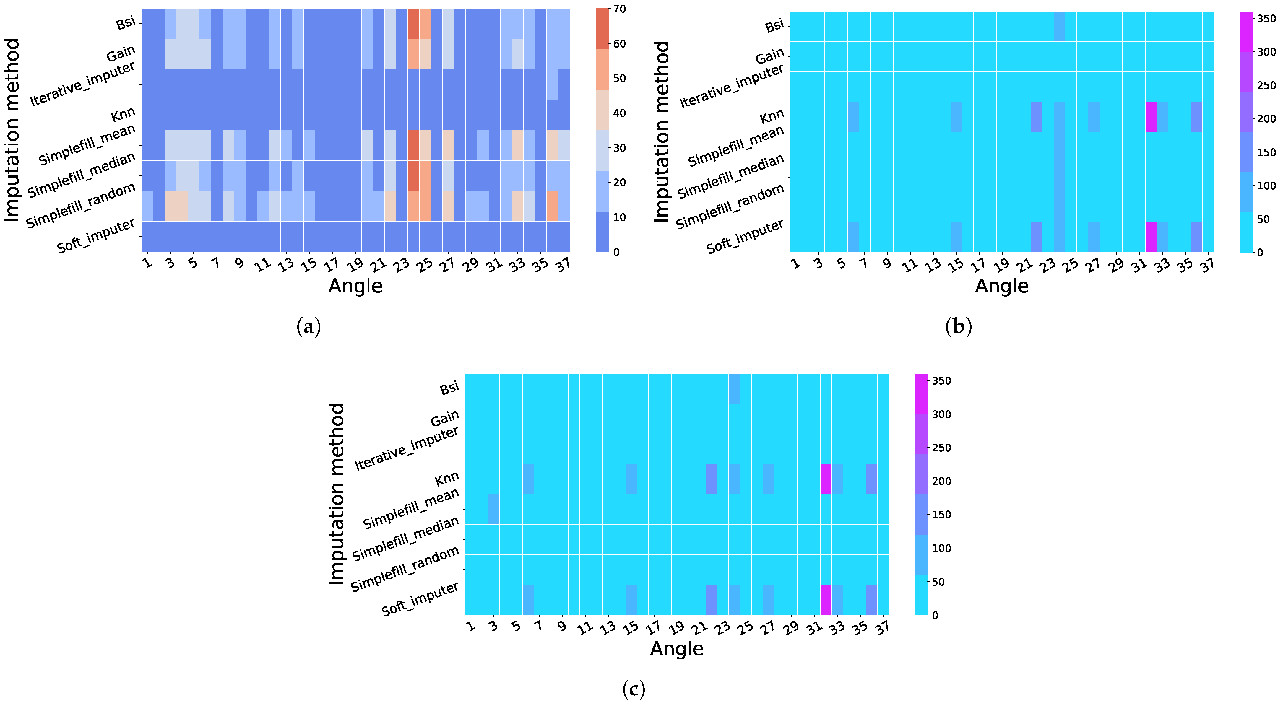
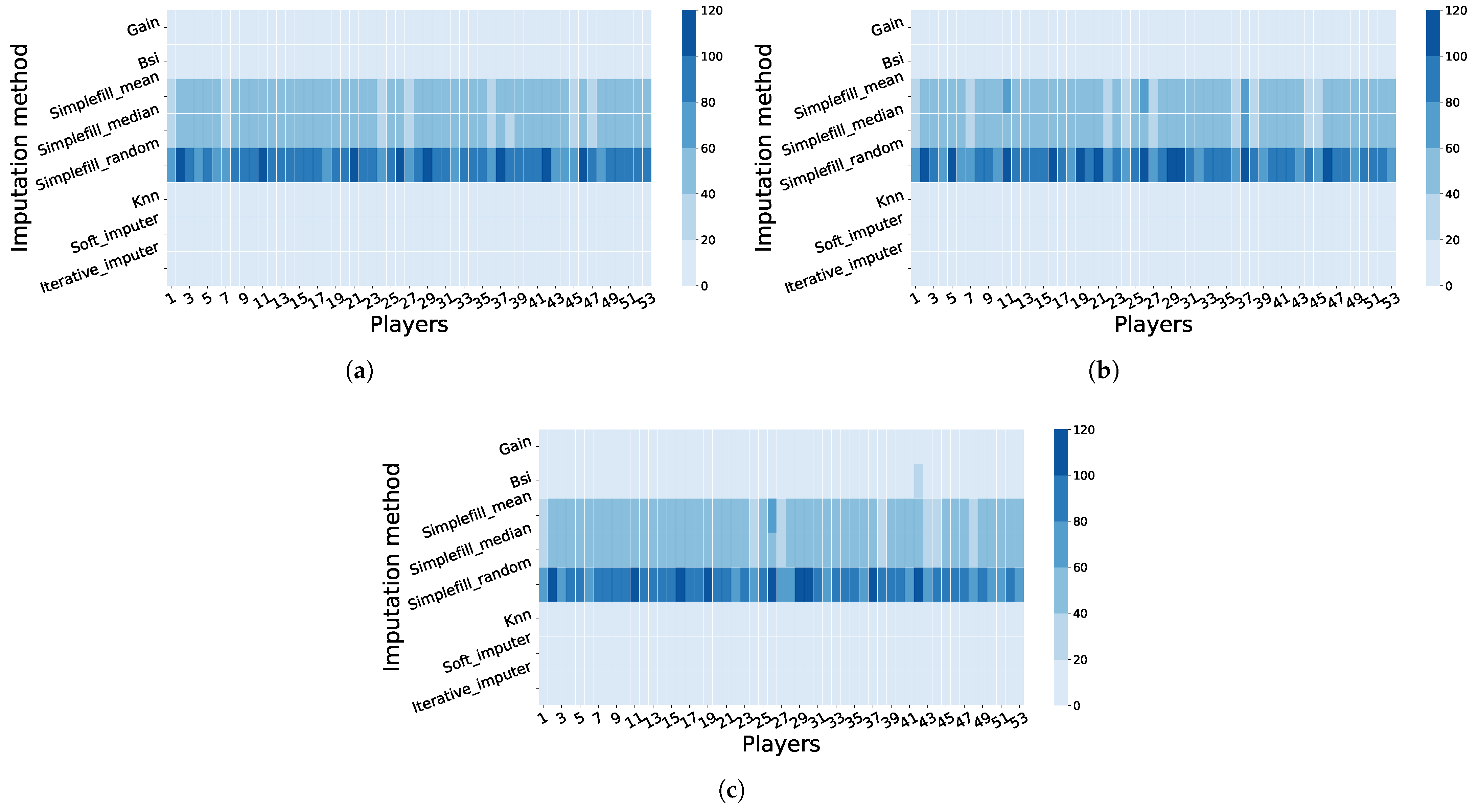
For randomly missing (MCAR) points, which were the simplest, there were some methods that functioned reasonably well. The Mean Absolute Error in Figure 3a is confined to a relatively low range, with the color bar selection ranging from 0 to 70. in this case, this is expected, as this scenario was both simple and could be interpolated with the adjacent temporal data points.
However, the challenge escalates significantly with more complex missingness. When the data is missing for critical transitions, Figure 3b shows the Mean Absolute Errors increased significantly, with the largest value associated with the MAE exceeding thresholds upwards of 350. This scenario clearly differentiates simple statistical methods from advanced models due to their critical interaction with time. The simple methods such as our SimpleFill Mean and SimpleFill Median perform poorly, as for both of these methods, their core mechanism—averaging—flattens the critical peaks and valleys that define the motion dynamics and creates a incorrect dependency only on this time series.
As shown in Figure 3c, the highest error values were observed in datasets with consecutive missing values located around transition points. This demonstrates, again, the difficult task of accurately imputing large portions of data. Observably, GAIN and Iterative Imputer, sophisticated models that learn nonlinear relationships within the sequence, performed better since they could utilize their complex modeling capacity to more effectively approximate the underlying dynamics of the sequence, thus significantly decreasing their mean error relative to simpler methods.
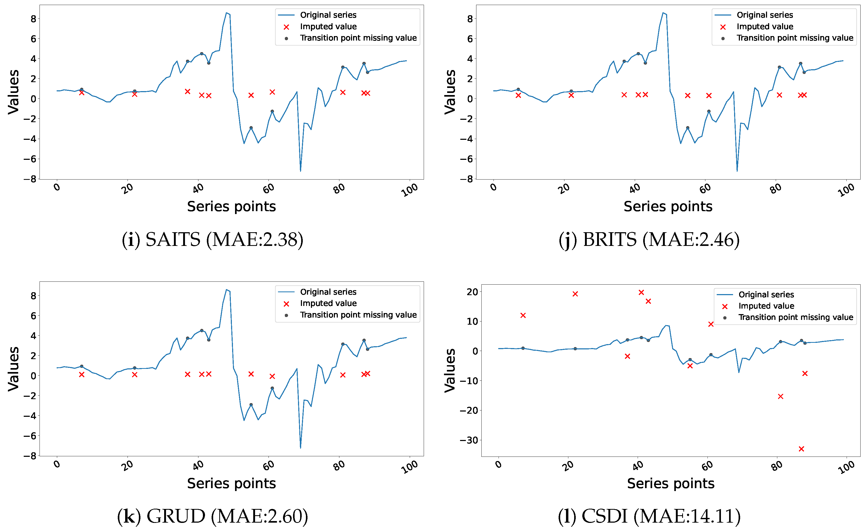
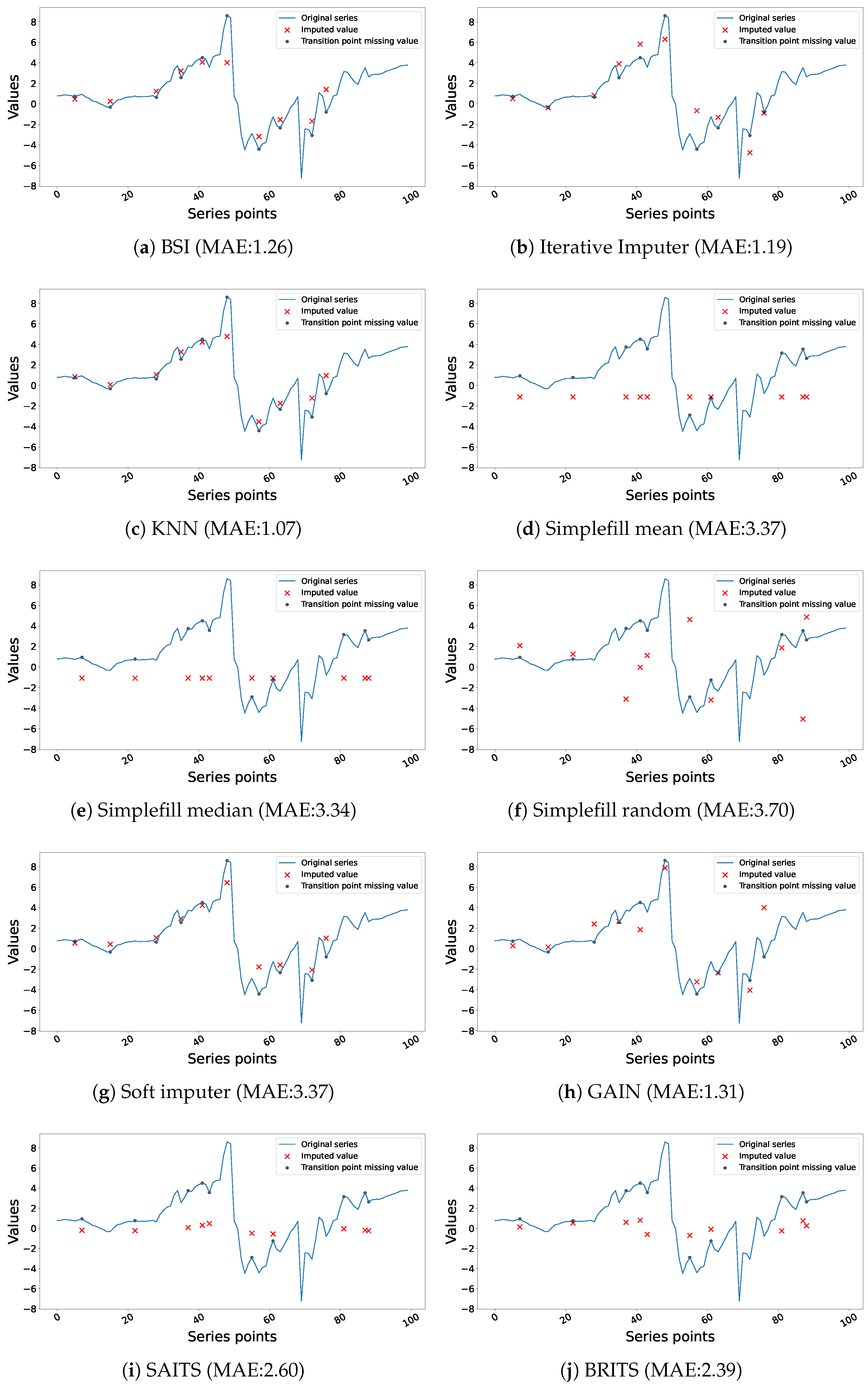
In summary, as the missing data conditions become more complex, the results of the error values across the datasets clearly show a trend of increasingly more difficult and erroneous data, as depicted in Figure 3. The ability of imputation techniques to replicate and adjust to the fundamental dynamics of the motion sequences largely determines their performance. When comparative external data was not available, more sophisticated techniques including GAIN and Iterative Imputer were able to manage the variance and complexity underlying intricate motion data. In summary, this study shows that although selecting simple imputation techniques based on the properties of the missing data may be crucial, more complicated approaches, such GAIN, have the possibility to improve the integrity of data reconstruction under challenging data conditions. Figure 4 depicts the true values against the imputed values for the utilized models. Figure 4l (i.e., CSDI) has a different visual scale than other figures in Figure 4a–k because there were higher error imputed values; thus, a greater range was required on the y-axis to display the data.
Table 1 lists the MAE values of several univariate imputation models applied to single player motion capture data. All listed results demonstrated the difficulty of reconstructing the missing data where no other data is utilized. The temporal models (SAITS, BRITS, GRU-D) specializing in time series analysis show the best performance, with an MAE under 8.0 for every missing data proportion explored. These models utilize temporal-aware architectures, firstly meant to operate on sequential data, while the other ML methods (i.e., KNN, Soft Imputer) display below-average performance at lower levels of missing data (i.e., data missing at 5%) before declining in performance at higher proportions of missing data. Statistical models using likelihood, most notably the Simplefill random, demonstrated worse performance relative to other types of models and consistently produced a worse level of error regardless of missing data %; this was as expected as they do not recognize the underlying biomechanical and temporal lay of movement data.
Notably, the CSDI model appears to exhibit significant variability and error rates relative to other DL models. The nature of the diffusion-based model remains important, but CSDI may be one additional deep learning technique that shows promise, requiring more adaptations to suit IMU-based motion capture data. The more traditional ML models and even DL methods such as GAIN and Iterative Imputer generated comparable levels of error to the majority of simple procedures with differing proportions of missing data, but they had high levels of inconsistencies when comparing their performance to various temporal models and limited missing data imputation processes.This analysis showcases the critical importance of temporal modeling features in univariate motion capture imputation processes in the absence of cross-sectional context, where imputation relies on a backlog of other player temporal data; its reliability depends on the imputation model.

4.2. Results and Comparative Interpretation of Multivariate Contexts

Switching from a univariate to a multivariate context provides auxiliary information to the imputation models, allowing their performance to be substantially enhanced. Our approach distinguishes between two multivariate scenarios: information from data of different players performing the same skill (motion) and information from data of different angles from the same player.

4.2.1. Across-Player Imputation: Results and Cohort-Based Interpretation

The multivariate player context assumes that for a given kinematic variable (angle), the time series from multiple players performing the same skill will exhibit common patterns. This is a powerful assumption in sports science and clinical studies involving standardized tasks.
We investigated formulating the problem as a multivariate imputation task by utilizing similar sequences within the data, thereby potentially improving the accuracy and dependability of imputation. This method enables us to use relationships and patterns across several variables in every sequence, thus providing a more informative context for imputing missing values. We sought to understand how different imputation techniques might take advantage of these interdependencies in scenarios spanning simple to highly complex missing data patterns by analyzing multivariate imputation across three datasets. In this experiment, we used the data of the same skill (motion) performed by several players to guide the imputation models to reconstruct the missing values for the players with missing motion data. The results of this experiment are listed in Table 2 and depicted in Figure 5.
In Table 2, one can observe substantial performance improvements between the univariate and multivariate cases. The time series deep learning models (i.e., SAITS, BRITS, GRU-D) yielded the best overall performance, with an MAE across all missing data percentages consistently below 3.2; this represents as much as a 70–80% improvement when compared to their univariate conditions. Traditional ML procedures such as KNN and Iterative Imputer provided moderate relative performance benefits, using cross-player correlations to reduce errors from their respective univariate baselines (for example, Iterative Imputer improved from 10.8 ± 6.9 to 5.82 ± 5.52 at 25% missing observations). However, statistical methods (Simplefill mean, median, and random) still performed poorly for the multivariate context, with only small improvements often varying considerably across missing data percentages. CSDI still had a considerable amount of variability with poor performance when compared to other DL methods, whereas GAIN did show moderate improvements but was less consistent than the specialized time series approaches. Overall, this analysis demonstrates that multimethod approaches lead to significant improvements in imputation accuracy by capitalizing on cohort-based correlations, with the largest gains resulting from models designed to capture spatio-temporal dependencies.
The vast majority of error values for the first dataset, randomly missing (MCAR) points, range roughly 0 to 20 as shown in Figure 5a. While methods such as SimpleFill Random, SimpleFill Mean, and SimpleFill Median performed well in most cases, they struggled with only one case (i.e., angle 36) where the error values ranged from 60 to 140. In the multivariate context, adding more information helped even simpler techniques like SimpleFill Mean and SimpleFill Median; this range shows that most approaches performed effectively. More advanced techniques such KNN and Iterative Imputer used the correlations between variables to provide more exact imputations, thus stressing the advantages of concurrently considering several variables.
With error values peaking at 140, the results of the second dataset, in which missing data was randomly distributed and at transition points, are depicted in Figure 5b. The second dataset was even more complex and emphasized the need for multivariate techniques such as Soft Imputer and Iterative Imputer. Both advanced methods took advantage of the complicated interrelationships between several variables, especially at transition points in the sequences where multiple variables are in motion; these methods had to account for the multivariate complexity of the data to discretely estimate the missing values. In contrast, the SimpleFill Random technique had a harder time with the increasing complexity and was more consistent with the higher error rates associated with simple method approaches. Comparing Figure 5 to Figure 3b, we note that the error range declines from 350 to 140; this reflects the importance of the auxiliary information, i.e., other players’ motion data, to the imputation models when improving error rates.
The results for the third dataset depicted in Figure 5c present substantial ranges of missing values even with transition points. Again, the highest error rate reduced to 140 from 350, which is the highest value of the same dataset using univariate imputation, as shown in Figure 3c. In cases where advanced methods like GAIN and Iterative Imputer can use their unique modeling powers to accurately reconstruct these portions of missing data, we noted that they performed the best, which was reassuring in that the extremely challenging continuity and accuracy of our imputed sequences relied on these methods’ management of the multivariate aspect of data.
Moving to a multivariate imputation framework significantly improves the imputation process, especially in complex scenarios. In a multivariate framework, multiple variables can be treated simultaneously, which further leverages the data available with the benefit of varying dimensions of detections. There is an emphasis, however, on selecting a method based on the dimensionality of the data, i.e., the the complexities of missingness across multiple variables. Multivariate imputation techniques will yield notable merits, being able to utilize and analyze the integrated data structures while maintaining the structural and dynamic integrity of complex data or datasets.
The increments in accuracy are explained in Table 1 and Table 2. For example, with 25% of data missing at transition points, the MAE for the Iterative Imputer reduced from 10.8 ± 6.9 (Table 1, Single-Player) to an improved 5.82 ± 5.52 (Table 2, Multi-Player). The MAE for the KNN imputer reduced from 12.0 ± 9.89 to 4.29 ± 7.06, which is close to a 50 percent improvement. This proves that if one player has a sensor that fails, the actions of other players provide useful information to guide the imputation model towards better imputed values of the missing data.
A graphical illustration of the imputed points and the true points for one case is presented in Figure 6. In Figure 6, the points imputed by the statistical-based methods are far from the true points, which indicates their weak performance, as shown in Figure 6d–f. In contrast, Figure 6a,c,h show accurate data imputation, as the distances between the imputed points and the true points are very small. The specialized deep learning models (i.e., SAITS, BRITS, GRUD) also exhibit consistently accurate reconstructions with low MAE values, but the CSDI exhibits poor performance (MAE » 3.0), with larger error validating the improved stability of the specialized time series approaches for the multivariate context (see Figure 6i–l).

4.2.2. Across-Angle Imputation: Results and Biomechanical Interpretation

The multivariate angle context was built upon the principle of biomechanical coupling: for one subject (person), the movement of one joint is dependent on the movements of other joints. This was the most impactful context, especially with structured data loss.
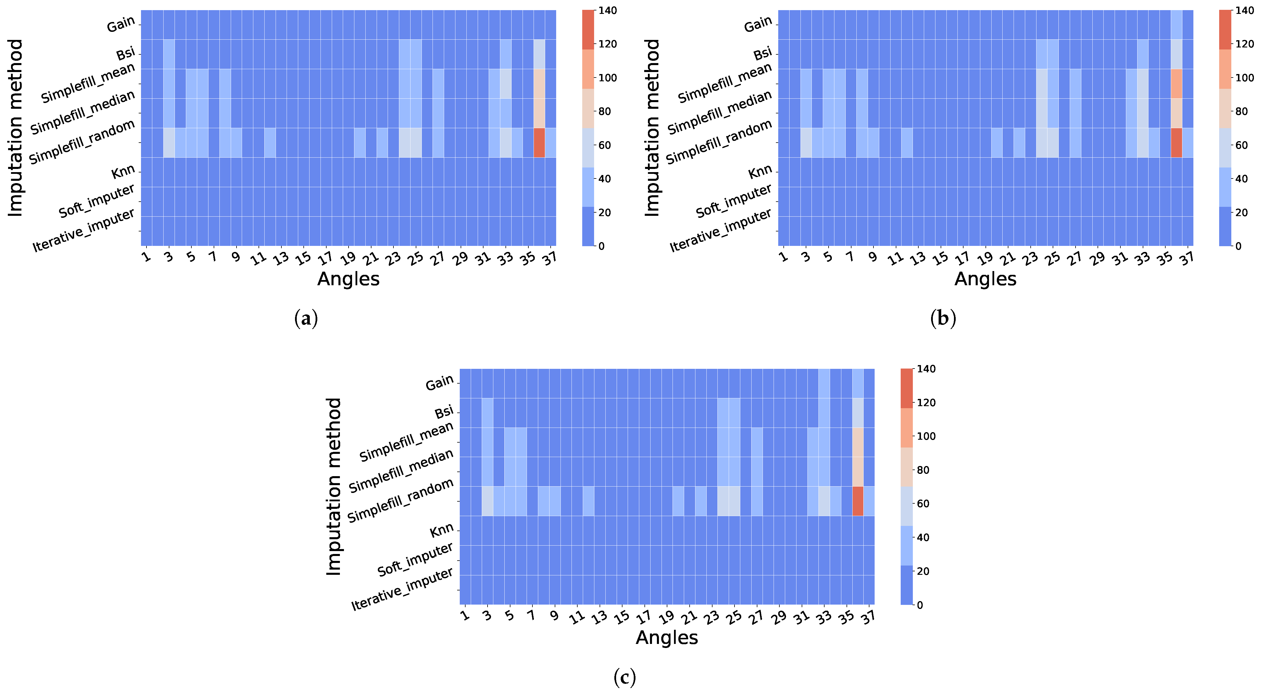
In the first dataset, sequences contained random missing values, and applying a univariate method resulted in an error range of 0 to 120, as depicted in Figure 7a. Although the multivariate approach increased the complexity of the imputation procedure, the performance of most of the non-statistical-based model significantly improved compared to the univariate results, as shown in Figure 3a. On the contrary, the statistical-based models’ performance declined. This behavior of model performance continued to appear in the other two datasets of missing values: the missing values around the transition points, as shown in Figure 7b, and the interval of missing values, as shown in Figure 7c.
The second dataset contained random discrete missing values and missing values at transition points in the sequences, which was a more complex scenario, where univariate missing value imputation methods yielded error values of 0–350. The use of multivariate imputation methods drastically improved the error values to 0–120, as shown in Figure 7b. This represents a more than 50% reduction in max error and supports the effectiveness of multivariate methods in utilizing relationships among multiple variables when confronted with complex patterns of missing data, especially at critical transition points in sequences.
The third dataset exhibited the most significant difficulties, with long intervals of missing values including transition points. Although the multivariate approach still produced high error values, peaking at 120 (as shown in Figure 7c), it was much better than the univariate results, thus illustrating the advanced powers of techniques such as GAIN and Iterative Imputer in a multivariate setting.
Generally, especially in complicated situations, the shift to a multivariate framework indicates a trend toward better imputation accuracy. Particularly where multivariate techniques can use inter-variable relationships to negotiate the complexity of missing data, thereby lowering error margins, the thorough comparison highlights great advantages. In disciplines like sports science, where exact data reconstruction is essential to the quality of performance analysis and consequent insights, this method is especially helpful.

4.3. Biomechanical Interpretation of Multivariate Gains

The superior performance of multivariate approaches within our benchmark analysis is consistent with the kinematic coupling between trunk and limbs during karate techniques. Angular velocities and linear accelerations at the shoulder, elbow, and wrist co-vary with pelvic and trunk rotation as torque is transferred proximally to distally. Multivariate angle contexts therefore help to preserve joint angle synergies during rotational movements, stabilizing peaks and transitions that univariate baselines tend to flatten. In multivariate player contexts, temporal consistency of acceleration profiles across sensor axes—a consequence of standardized elite instruction—provides strong priors for plausible trajectories at a given angle. Model-specific iterative multivariate imputers exploit cross-feature regression on aligned angles, while adversarial and attention-based models (e.g., GAIN’s ability to model latent dependencies between IMU streams) leverage long-range temporal structure to maintain physically consistent reconstructions through ballistic phases and re-grasping phases.

4.4. Discussion

Our empirical investigation first identified severe limitations in treating MoCap time series as either merely sequences of observations or as univariate series. In this context, the imputation performance is critically dependent on the missingness mechanism, as, for example, some simple, randomly missing points may reasonably interpolate from each side of the temporal sequence; however, for more complex structures, performance degrades severely. The failure of simple statistics methods on missing transitional points is particularly telling and reinforces the nature of methods like mean filling, which “flatten” some of the important peaks and valleys in the dynamics of the movement, thereby creating possibly unacceptable distortions. The extent to which this limitation was compounded in terms of instability for representative motions with block missingness, where there were no local conditions to view the interpolulated motion, forced the model to extrapolate without guidance and therefore resulted in fundamentally unreliable imputations, leading to fundamentally unreliable imputations.
The multivariate frameworks offered a way to mitigate this issue by using critical auxiliary information, with the across-player context also performing well in incident-related data loss. This context leverages cohort similarities and is predicated on assumptions that the different players possess common motions in certain skilled aspects. The model effectively learns a statistically shared template or archetype for the skill movement itself by drawing information from a distribution of performances. A key observation is that when a player’s sensor failed at a key incident in the movement (e.g., peak, valley), the equivalent motion from other players provided an excellent, high-fidelity basis for reconstructing the movement, explaining the significant error reduction for missing transition points.
Based on the varieties of the missing measurements, the multivariate angle context consistently achieved the best performance, simply because it is the model most suited to the nature of MoCap data. The framework’s ability to model the intrinsic biomechanical coupling of the human kinematic chain meant that in that context, it was very effective. For instance, one joint (e.g., elbow) should have one state based on the states of the adjacent joints (e.g., shoulder and wrist). This context is particularly powerful when considering contiguous block missingness as well, because it is true that while temporal information is lost for one channel, the cross-sectional kinematic relationships with all other channels are intact for every time step. In short, this offers an ongoing and structural basis for reconstructing data that the other contexts cannot provide when there is structured data loss.
It is challenging to synthesize these results to propose a clear hierarchy of imputation strategies predicated on the correlation type being exploited. The findings demonstrate that the imputation context is not arbitrary; it is a critical modeling decision that encodes assumptions about the structure of the data. Second, when a subject has multi-joint data available, it is obviously better to use the across-angle context because of its use of physically constrained data.In contrast, the across-player context is a useful alternative for single-angle analysis across a cohort; it may be better than designated parameters in this context and the across-player context.Lastly, for univariate contexts, it is limited to that instance in which there is no other correlated data, with the explicit understanding of its vulnerability to structured data loss.
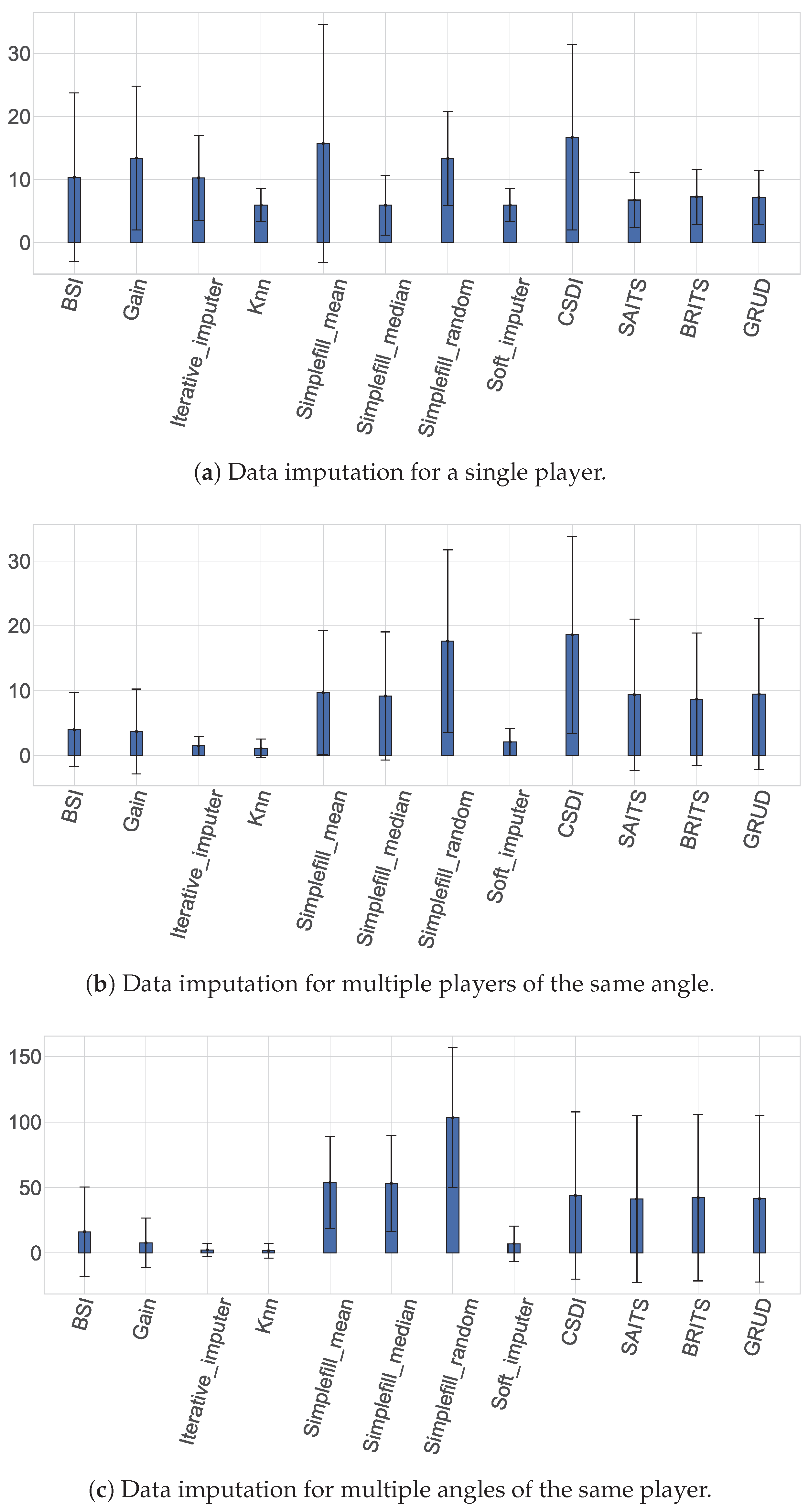
A direct comparison of the error bar plots for the transition point missingness mechanism shows a significant difference in imputation performance across the three contexts and underlines the importance of the correlation of the data itself, as shown in Figure 8. In the univariate and multivariate multi-player contexts, advanced models (e.g., Iterative Imputer and KNN) achieve much better performance than basic statistical models, with an MAE of around 1–5. Of note, the specialized time series deep learning models (i.e., SAITS, BRITS, GRUD) show consistently superior performance, with MAE values below 3 across all contexts, while CSDI shows higher variability but still surpasses traditional statistical methods. Due to large variance in Simplefill mean and Simplefill random, the error bars extend to an MAE of over 30 in some cases. Thus, using these statistical methods is risky for dynamically important data. However, performance characteristics shift dramatically when moving to the multi-angle context. In the multi-angle context, advanced models that can leverage biomechanically coupled kinematic variables and achieve an MAE of around zero with very little variance (indicating perfect reconstruction), with the specialized deep learning models maintaining their superior stability. Meanwhile, simple statistical-based methods fail catastrophically, with Simplefill random demonstrating an MAE of over 100. This makes sense because they these methods perform a physically incongruous operation of averaging across distinct and dynamically different angles (e.g., of the shoulder and wrist), which results in a physically impossible data ranges and very large errors. This demonstrates that the choice of imputation method is as critical as the availability of data, as an incongruous approach can negate the benefits of a richer dataset and compromise the trustworthiness of the results.
The enhanced performance of the Iterative Imputer and GAIN methods at transition points can be understood based on their design and mechanisms of operation. These methods can model nonlinear temporal dependencies within each time series with biomechanical coupling to multiple joints. Consequently, the two methods were able to produce physically consistent kinematic sequences with nonlinear transitions during quick fluctuations/changes in motion (i.e., peak and valley) when applying these methods.Conversely, even the simple statistical approach (mean or median filling) was unable to capture cross-joint correlation and nonlinear dynamics, which flattened the important transitions and generated large errors at change points, because it relied on a single imputation from a likelihood model and did not model any cross-joint correlation.

4.5. Study Limitations and Implications for Future Work

A limitation of this work is that we did not perform missing not at random (MNAR) scenarios or dynamic (i.e., time-dependent) missingness approaches, and we did not use any multimodal signals (e.g., electromyographic (EMG)). Generally speaking, while our benchmark focused on MCAR, transition-based block structures (missing-at-random forms of treatment), MNAR, and non-stationary missingness are very relevant in practice, and therefore so are the complexities of cross-modal interpolation. These were not experimented with in this part of the work due to its scope, but we recognize that they are important, and we have identified them as important directions in future extensions to the benchmark. Furthermore, our benchmark was based solely on IMU-based MoCap data. Extending the framework into further domains such as medical time series (e.g., EEG) and financial domains would serve to assess the transferability of the techniques we have proposed into further application domains. We believe this is an important area of future work for more generalizable findings.
One additional limitation of this work is that we did not consider hybrid models, such as traditional methods followed by deep learning methods (e.g., KNN pre-filling followed by GAN), which may benefit from both methods’ compounded properties. Further, hyperparameter tuning—for example, running a grid search for Iterative Imputer iterations, or GAIN’s generator configurations—could produce enhanced performance. However, we also consider these as future directions for future applications of this framework. Although the MAE was chosen for its ease of interpretation and uniformity across methods, we acknowledge that the MAE does not measure temporal alignment or structural consistency; therefore, future additions will include relevant metrics like Dynamic Time Warping distance and joint-angle-based errors rather than position-based errors.
The primary limitation of this work is the uniformity of the dataset: all 53 subjects were elite adult male participants. The lack of demographic variability (age, gender, rank, and anthropometrics) is likely to limit the transferability or generalizability of our findings. Beginners or less elite players may exhibit more inter-trial variability, which may change how difficult imputation is to perform. Moreover, while there are four skills in the dataset, we only used the Gedan Barai skill for this analysis due to space constraints. Future research should involve larger movement repertoires including a more heterogeneous population to investigate the robustness of imputation approaches.

5. Conclusions

This work provides a broad introduction to data imputation with missing data within the area of motion capture through IMU sensors, an area in which data quality is important. We were able to perform the first exhaustive comparison of statistical methods, machine learning methods, and deep learning methods across three new imputation contexts: univariate, multivariate players, and multivariate angles. Specifically, in the multivariate angle context, advanced methods like the Iterative Imputer and KNN achieved a 64% reduction in MAE (from 12.0 ± 9.89 to 4.29 ± 7.06) by leveraging multi-player information. The utilization of time series DL models (i.e., SAITS, BRITS, GRU-D) consistently achieved 50–80% better accuracy than traditional approaches across all experimental conditions. A key contribution of this paper is the introduction of the first publicly available benchmark dataset to help standardize the evaluation of imputation methods for this unique time series data. All our experimental findings are clear. We show that multivariate frameworks that exploit the correlations across players or kinematic variables are far superior to univariate approaches, especially with unusual patterns of missingness. The more sophisticated models such as GAIN and the Iterative Imputer produced the highest quality data imputation—these are the best models for capturing the complex aspects of human motion. The scale of the dataset (53 subjects, 100 time points) may limit the capacity of our findings to be generalized to sequences that are longer or have more diverse movements. One key limitation of this study is that the motion capture is restricted to four specific skills performed by Karate practitioners; however, it provided a controlled setting in which to analyze the proposed imputation methods. The work we have undertaken has created an acceptable baseline and defined the most apparent next steps through which to support future researchers. Based on our findings, we suggest the following: (1) prioritization of specialized time series models (i.e., SAITS, BRITS, GRU-D) for optimal performance across all contexts; (2) use of a multivariate angle context when complete kinematic data is accessible; (3) use of Iterative Imputer or GAIN as secondary options when specialized models are unavailable; and (4) avoidance of simple statistical methods for dynamic transition points, as they can significantly compromise reconstruction quality. Our results indicate that specialized time series models (SAITS, BRITS, GRU-D) perform optimally across all missing rates (5–30%) and contexts, while traditional methods like Iterative Imputer and GAIN serve as viable alternatives when there are moderate missing rates (≤30%), especially in multivariate contexts. Future researchers should focus on transparent validation studies when working with real observations that will have naturally occurring gaps. While this work considered only IMU-derived kinematic signals, the multimodal extension combining IMU with EMG recordings represents an important opportunity for future research. Cross-modal imputation may result in stronger imputations through complementary information from multiple detection modalities. Future benchmark datasets and studies should therefore explicitly include multimodal data to increase the robustness and applicability of imputation methods in human motion analysis.

Author Contributions

Conceptualization, M.B. and A.S.; methodology, M.B.; software, T.A. and A.F.; validation, A.F.; formal analysis, A.S.A. and A.F.; investigation, E.E.; resources, A.A.; data curation, A.F.; writing—original draft preparation, M.B., A.S.A. and E.E.; writing—review and editing, A.S.A., A.S., A.F. and E.E.; visualization, M.B.; supervision, A.S., A.S.A. and A.F.; project administration, A.A.; funding acquisition, A.S. and A.S.A. All authors have read and agreed to the published version of the manuscript.

Funding

This work was supported by a research grant from the Omani Ministry of Higher Education Research Innovation (MOHERI) under the project number BFP/RGP/ICT/23/382.

Institutional Review Board Statement

Not applicable.

Informed Consent Statement

Not applicable.

Data Availability Statement

The original data presented in the study are openly available in GitHub at https://github.com/stars-of-orion/MoCap-Impute (accessed on 1 August 2025).

Conflicts of Interest

Author Tarek Attia was employed by Wakeb. The remaining authors declare that the research was conducted in the absence of any commercial or financial relationships that could be construed as a potential conflict of interest.

References

  1. Van der Kruk, E.; Reijne, M.M. Accuracy of human motion capture systems for sport applications; state-of-the-art review. Eur. J. Sport Sci. 2018, 18, 806–819. [Google Scholar] [CrossRef]
  2. Fathalla, A.; Salah, A.; Bekhit, M.; Eldesouky, E.; Talha, A.; Zenhom, A.; Ali, A. Real-Time and Automatic System for Performance Evaluation of Karate Skills Using Motion Capture Sensors and Continuous Wavelet Transform. Int. J. Intell. Syst. 2023, 2023, 1561942. [Google Scholar] [CrossRef]
  3. Jalata, I.K.; Truong, T.D.; Allen, J.L.; Seo, H.S.; Luu, K. Movement analysis for neurological and musculoskeletal disorders using graph convolutional neural network. Future Internet 2021, 13, 194. [Google Scholar] [CrossRef]
  4. Arlotti, J.S.; Carroll, W.O.; Afifi, Y.; Talegaonkar, P.; Albuquerque, L.; Ball, J.E.; Chander, H.; Petway, A. Benefits of IMU-based Wearables in Sports Medicine: Narrative Review. Int. J. Kinesiol. Sport. Sci. 2022, 10, 36–43. [Google Scholar] [CrossRef]
  5. Adel, B.; Badran, A.; Elshami, N.E.; Salah, A.; Fathalla, A.; Bekhit, M. A Survey on Deep Learning Architectures in Human Activities Recognition Application in Sports Science, Healthcare Security. In Proceedings of the the International Conference on Innovations in Computing Research, Athens, Greece, 5–7 July 2022; pp. 121–134. [Google Scholar]
  6. Ismail, A.R.; Zainal Abidin, N.; Maen, M.K. Systematic Review on Missing Data Imputation Techniques with Machine Learning Algorithms for Healthcare. J. Robot. Control (JRC) 2022, 3, 143–152. [Google Scholar] [CrossRef]
  7. Kaseris, M.; Kostavelis, I.; Malassiotis, S. A Comprehensive Survey on Deep Learning Methods in Human Activity Recognition. Mach. Learn. Knowl. Extr. 2024, 6, 842–876. [Google Scholar] [CrossRef]
  8. Guignard, B.; Ayad, O.; Baillet, H.; Mell, F.; Simbaña Escobar, D.; Boulanger, J.; Seifert, L. Validity, reliability and accuracy of inertial measurement units (IMUs) to measure angles: Application in swimming. Sport. Biomech. 2021, 23, 1471–1503. [Google Scholar] [CrossRef]
  9. Wang, L.; Sun, Y.; Li, Q.; Liu, T.; Yi, J. Two shank-mounted IMUs-based gait analysis and classification for neurological disease patients. IEEE Robot. Autom. Lett. 2020, 5, 1970–1976. [Google Scholar] [CrossRef]
  10. Karuzaki, E.; Partarakis, N.; Patsiouras, N.; Zidianakis, E.; Katzourakis, A.; Pattakos, A.; Kaplanidi, D.; Baka, E.; Cadi, N.; Magnenat-Thalmann, N.; et al. Realistic virtual humans for cultural heritage applications. Heritage 2021, 4, 4148–4171. [Google Scholar] [CrossRef]
  11. Yahya, M.; Shah, J.A.; Kadir, K.A.; Yusof, Z.M.; Khan, S.; Warsi, A. Motion capture sensing techniques used in human upper limb motion: A review. Sens. Rev. 2019, 39, 504–511. [Google Scholar] [CrossRef]
  12. Clemente, F.M.; Akyildiz, Z.; Pino-Ortega, J.; Rico-González, M. Validity and reliability of the inertial measurement unit for barbell velocity assessments: A systematic review. Sensors 2021, 21, 2511. [Google Scholar] [CrossRef] [PubMed]
  13. Ahmad, N.; Ghazilla, R.A.R.; Khairi, N.M.; Kasi, V. Reviews on various inertial measurement unit (IMU) sensor applications. Int. J. Signal Process. Syst. 2013, 1, 256–262. [Google Scholar] [CrossRef]
  14. Behrmann, N.; Hillebrecht, M.; Pöppl, N.; Pöppl, S.; Seiler, S. Is the EnodePro® a Valid Tool to Determine the Bar Velocity in the Bench Press and Barbell Back Squat? A Comparative Analysis. Sensors 2025, 25, 549. [Google Scholar] [CrossRef] [PubMed]
  15. Dragutinovic, S.; Djuric, S.; Petruzzi, S. Validation of the VmaxPro Sensor for Assessing Velocity and Load-Velocity Variables During Back Squat and Bench Press Exercises. Sports 2024, 12, 101. [Google Scholar] [CrossRef]
  16. Zhu, R.; Zhou, Z. A real-time articulated human motion tracking using tri-axis inertial/magnetic sensors package. IEEE Trans. Neural Syst. Rehabil. Eng. 2004, 12, 295–302. [Google Scholar]
  17. Cai, Q.; Song, N.; Yang, G.; Liu, Y. Accelerometer calibration with nonlinear scale factor based on multi-position observation. Meas. Sci. Technol. 2013, 24, 105002. [Google Scholar] [CrossRef]
  18. Zhang, X.; Zhou, C.; Chao, F.; Lin, C.M.; Yang, L.; Shang, C.; Shen, Q. Low-cost inertial measurement unit calibration with nonlinear scale factors. IEEE Trans. Ind. Inform. 2021, 18, 1028–1038. [Google Scholar] [CrossRef]
  19. Sohrabi, H.; Ebadollahi, S. Accuracy enhancement of MEMS accelerometer by determining its nonlinear coefficients using centrifuge test. Measurement 2017, 112, 29–37. [Google Scholar] [CrossRef]
  20. Olivares, A.; Olivares, G.; Gorriz, J.; Ramirez, J. High-efficiency low-cost accelerometer-aided gyroscope calibration. In Proceedings of the 2009 International Conference on Test and Measurement, Hong Kong, China, 5–6 December 2009; Volume 1, pp. 354–360. [Google Scholar]
  21. Kozlov, A.; Sazonov, I.; Vavilova, N. IMU calibration on a low grade turntable: Embedded estimation of the instrument displacement from the axis of rotation. In Proceedings of the 2014 International Symposium on Inertial Sensors and Systems (ISISS), Laguna Beach, CA, USA, 25–26 February 2014; pp. 1–4. [Google Scholar]
  22. Aktakka, E.E.; Woo, J.K.; Najafi, K. On-chip characterization of scale-factor of a MEMS gyroscope via a micro calibration platform. In Proceedings of the 2017 IEEE International Symposium on Inertial Sensors and Systems (INERTIAL), Kauai, HI, USA, 27–30 March 2017; pp. 1–4. [Google Scholar]
  23. Renner, J.; Rumpf, M.C.; Wagner, M.; Zoch, M.; Pöppl, S. Concurrent Validity of Novel Smartphone-Based Apps Monitoring Barbell Velocity in Powerlifting Exercises. Sensors 2024, 24, 882. [Google Scholar] [CrossRef]
  24. Tashiro, Y.; Song, J.; Song, Y.; Ermon, S. Csdi: Conditional score-based diffusion models for probabilistic time series imputation. Adv. Neural Inf. Process. Syst. 2021, 34, 24804–24816. [Google Scholar]
  25. Adhikari, D.; Jiang, W.; Zhan, J.; He, Z.; Rawat, D.B.; Aickelin, U.; Khorshidi, H.A. A comprehensive survey on imputation of missing data in internet of things. ACM Comput. Surv. 2022, 55, 1–38. [Google Scholar] [CrossRef]
  26. Hasan, M.K.; Alam, M.A.; Roy, S.; Dutta, A.; Jawad, M.T.; Das, S. Missing value imputation affects the performance of machine learning: A review and analysis of the literature (2010–2021). Inform. Med. Unlocked 2021, 27, 100799. [Google Scholar] [CrossRef]
  27. Luo, Y. Evaluating the state of the art in missing data imputation for clinical data. Briefings Bioinform. 2022, 23, bbab489. [Google Scholar] [CrossRef]
  28. Singh, G.; Jaiswal, A.K. Efficient Imputation Methods to Handle Missing Data in Sample Surveys. J. Stat. Theory Pract. 2022, 16, 40. [Google Scholar] [CrossRef]
  29. Donders, A.R.T.; Van Der Heijden, G.J.; Stijnen, T.; Moons, K.G. A gentle introduction to imputation of missing values. J. Clin. Epidemiol. 2006, 59, 1087–1091. [Google Scholar] [CrossRef] [PubMed]
  30. Lin, W.C.; Tsai, C.F. Missing value imputation: A review and analysis of the literature (2006–2017). Artif. Intell. Rev. 2020, 53, 1487–1509. [Google Scholar] [CrossRef]
  31. Little, T.D.; Jorgensen, T.D.; Lang, K.M.; Moore, E.W.G. On the joys of missing data. J. Pediatr. Psychol. 2014, 39, 151–162. [Google Scholar] [CrossRef] [PubMed]
  32. Leurent, B.; Gomes, M.; Faria, R.; Morris, S.; Grieve, R.; Carpenter, J.R. Sensitivity analysis for not-at-random missing data in trial-based cost-effectiveness analysis: A tutorial. Pharmacoeconomics 2018, 36, 889–901. [Google Scholar] [CrossRef]
  33. de Goeij, M.C.; van Diepen, M.; Jager, K.J.; Tripepi, G.; Zoccali, C.; Dekker, F.W. Multiple imputation: Dealing with missing data. Nephrol. Dial. Transplant. 2013, 28, 2415–2420. [Google Scholar] [CrossRef]
  34. Bakar, A.A.; Ahmad, I.B.; Yusof, Y.S.; Zakaria, I.H.; Yacob, H. A hybrid CNN-LSTM model with attention mechanism for missing data imputation. Artif. Intell. Med. 2023, 145, 102587. [Google Scholar] [CrossRef]
  35. Rubin, D.B. Multiple Imputation for Nonresponse in Surveys; John Wiley & Sons: Hoboken, NJ, USA, 2004; Volume 81. [Google Scholar]
  36. Kang, J.; Yuan, Y.; Emery, C. Assessing remedies for missing weekly individual exposure in sport injury studies. Inj. Prev. 2014, 20, 177–182. [Google Scholar] [CrossRef]
  37. Wood, A.M.; White, I.R.; Hillsdon, M.; Carpenter, J. Comparison of imputation and modelling methods in the analysis of a physical activity trial with missing outcomes. Int. J. Epidemiol. 2005, 34, 89–99. [Google Scholar] [CrossRef]
  38. Jekauc, D.; Völkle, M.; Lämmle, L.; Woll, A. Missing values in sport scientific studies: A practical guide to multiple imputation with SPSS. Sportwissenschaft 2012, 42, 126–136. [Google Scholar] [CrossRef]
  39. Wang, C.; Stokes, T.; Steele, R.; Wedderkopp, N.; Shrier, I. Implementing multiple imputation for missing data in longitudinal studies when models are not feasible: A tutorial on the random hot deck approach. arXiv 2020, arXiv:2004.06630. [Google Scholar] [CrossRef]
  40. Solaro, N.; Barbiero, A.; Manzi, G.; Ferrari, P. A simulation comparison of imputation methods for quantitative data in the presence of multiple data patterns. J. Stat. Comput. Simul. 2018, 88, 3588–3619. [Google Scholar] [CrossRef]
  41. Takahashi, M. Multiple ratio imputation by the EMB algorithm: Theory and simulation. J. Mod. Appl. Stat. Methods 2017, 16, 34. [Google Scholar] [CrossRef]
  42. Jang, J.H.; Choi, J.; Roh, H.W.; Son, S.J.; Hong, C.H.; Kim, E.Y.; Kim, T.Y.; Yoon, D. Deep learning approach for imputation of missing values in actigraphy data: Algorithm development study. JMIR MHealth UHealth 2020, 8, e16113. [Google Scholar] [CrossRef] [PubMed]
  43. Singh, M.S.; Thongam, K.; Choudhary, P.; Bhagat, P. An integrated machine learning approach for congestive heart failure prediction. Diagnostics 2024, 14, 736. [Google Scholar] [CrossRef]
  44. Benson, L.C.; Stilling, C.; Owoeye, O.B.; Emery, C.A. Evaluating methods for imputing missing data from longitudinal monitoring of athlete workload. J. Sport. Sci. Med. 2021, 20, 188. [Google Scholar] [CrossRef]
  45. Hammerling, D.; Cefalu, M.; Cisewski, J.; Dominici, F.; Parmigiani, G.; Paulson, C.; Smith, R.L. Completing the results of the 2013 Boston marathon. PLoS ONE 2014, 9, e93800. [Google Scholar] [CrossRef]
  46. Kato, T.; Kasugai, R.; Sakai, K. Relationship Between the Total Quality Recovery Scale and Race Performance in Competitive College Swimmers over Two Seasons. Sports 2025, 13, 139. [Google Scholar] [CrossRef]
  47. Barker, J.; McCarthy, P.; Jones, M.; Moran, A. Single-Case Research Methods in Sport and Exercise Psychology; Routledge: London, UK, 2011. [Google Scholar]
  48. Ramli, M.N.; Yahaya, A.S.; Ramli, N.; Yusof, N.F.F.M.; Abdullah, M. Roles of imputation methods for filling the missing values: A review. Adv. Environ. Biol. 2013, 7, 3861–3870. [Google Scholar]
  49. Ette, E.I.; Chu, H.M.; Ahmad, A. Data Imputation; John Wiley & Sons: Hoboken, NJ, USA, 2006; pp. 245–262. [Google Scholar] [CrossRef]
  50. Kishore, C.L.; Rao, C.R. A Comparative Study on Missing Value Imputation Techniques in Machine Learning. In Proceedings of the SHS Web of Conferences, Paris, France, 20–22 May 2025; Volume 218, p. 02014. [Google Scholar] [CrossRef]
  51. Alwateer, M.; Atlam, E.S.; Abd El-Raouf, M.M.; Ghoneim, O.A.; Gad, I. Missing data imputation: A comprehensive review. J. Comput. Commun. 2024, 12, 53–75. [Google Scholar] [CrossRef]
  52. Ser, G.; Keskin, S.; Yilmaz, M. The performance of multiple imputations for different number of imputations. Sains Malays. 2016, 45, 1755–1761. [Google Scholar]
  53. Sterne, J.A.; White, I.R.; Carlin, J.B.; Spratt, M.; Royston, P.; Kenward, M.G.; Wood, A.M.; Carpenter, J.R. Multiple imputation for missing data in epidemiological and clinical research: Potential and pitfalls. Bmj 2009, 338, b2393. [Google Scholar] [CrossRef] [PubMed]
  54. Mistler, S.A.; Enders, C.K. A comparison of joint model and fully conditional specification imputation for multilevel missing data. J. Educ. Behav. Stat. 2017, 42, 432–466. [Google Scholar] [CrossRef]
  55. Zhang, L.C. Nonparametric Markov chain bootstrap for multiple imputation. Comput. Stat. Data Anal. 2004, 45, 343–353. [Google Scholar] [CrossRef]
  56. White, I.R.; Daniel, R.; Royston, P. Avoiding bias due to perfect prediction in multiple imputation of incomplete categorical variables. Comput. Stat. Data Anal. 2010, 54, 2267–2275. [Google Scholar] [CrossRef]
  57. Ae Lee, J.; Gill, J. Missing value imputation for physical activity data measured by accelerometer. Stat. Methods Med Res. 2018, 27, 490–506. [Google Scholar] [CrossRef]
  58. Nguyen, Q.; Matthews, G.J. Filling the gaps: A multiple imputation approach to estimating aging curves in baseball. J. Sport. Anal. 2024, 10, 77–85. [Google Scholar] [CrossRef]
  59. Epp-Stobbe, A.; Tsai, M.-C.; Klimstra, M. Comparison of Imputation Methods for Missing Rate of Perceived Exertion Data in Rugby. Mach. Learn. Knowl. Extr. 2022, 4, 827–838. [Google Scholar] [CrossRef]
  60. Woods, A.D.; Gerasimova, D.; Van Dusen, B.; Nissen, J.; Bainter, S.; Uzdavines, A.; Davis-Kean, P.E.; Halvorson, M.; King, K.M.; Logan, J.A.; et al. Best practices for addressing missing data through multiple imputation. Infant Child Dev. 2024, 33, e2407. [Google Scholar] [CrossRef]
  61. Li, P.; Stuart, E.A.; Allison, D.B. Multiple imputation: A flexible tool for handling missing data. JAMA 2015, 314, 1966–1967. [Google Scholar] [CrossRef]
  62. Muzellec, B.; Josse, J.; Boyer, C.; Cuturi, M. Missing data imputation using optimal transport. In Proceedings of the International Conference on Machine Learning, Vienna, Austria, 12–18 July 2020; pp. 7130–7140. [Google Scholar]
  63. Du, W.; Côté, D.; Liu, Y. Saits: Self-attention-based imputation for time series. Expert Syst. Appl. 2023, 219, 119619. [Google Scholar] [CrossRef]
  64. Cao, W.; Wang, D.; Li, J.; Zhou, H.; Li, L.; Li, Y. Brits: Bidirectional recurrent imputation for time series. Adv. Neural Inf. Process. Syst. 2018, 31, 6776–6786. [Google Scholar]
  65. Che, Z.; Purushotham, S.; Cho, K.; Sontag, D.; Liu, Y. Recurrent neural networks for multivariate time series with missing values. Sci. Rep. 2018, 8, 6085. [Google Scholar] [CrossRef]
  66. Yoon, J.; Jordon, J.; Schaar, M. Gain: Missing data imputation using generative adversarial nets. In Proceedings of the International Conference on Machine Learning, Stockholm, Sweden, 10–15 July 2018; pp. 5689–5698. [Google Scholar]
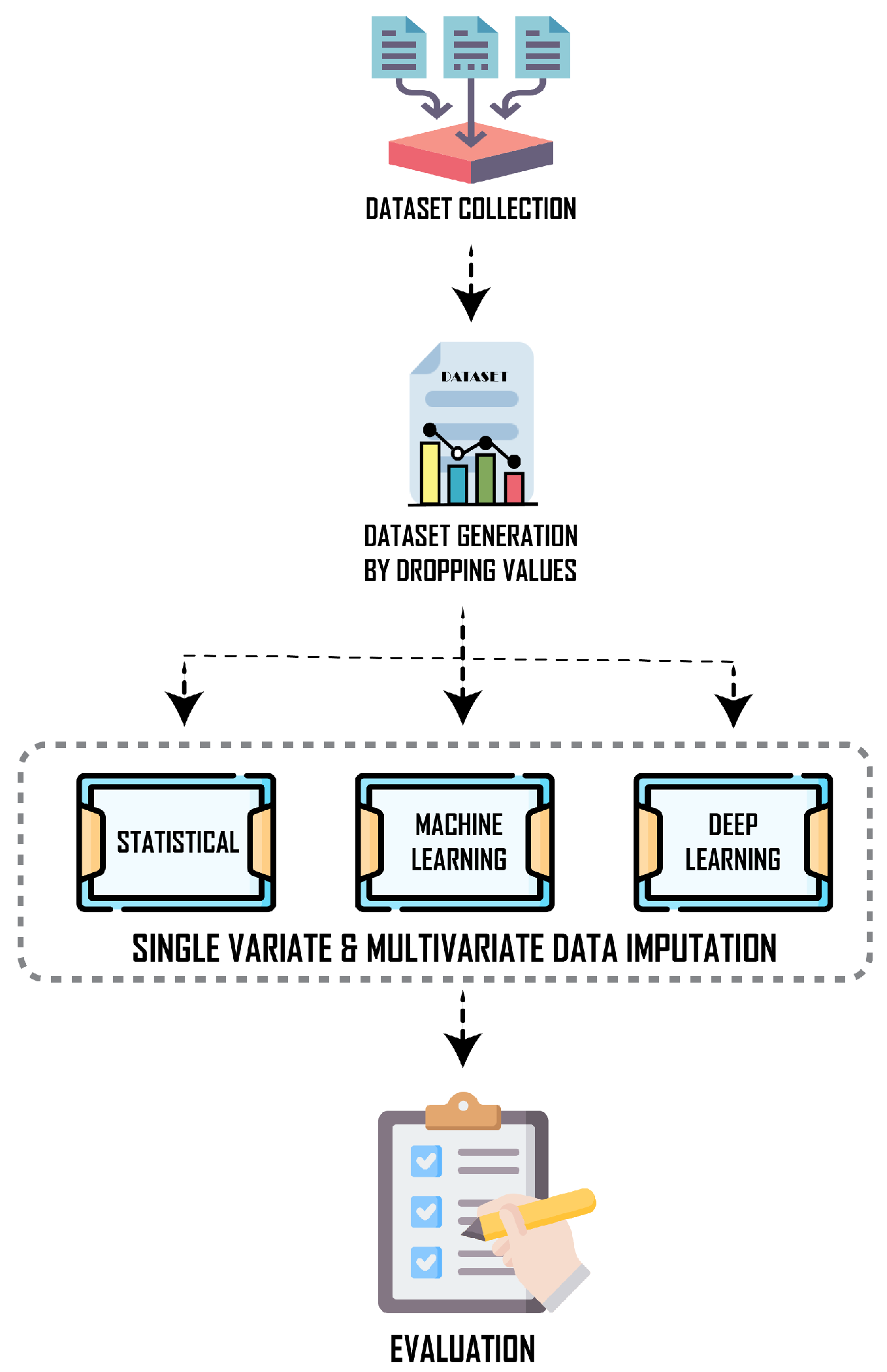
Figure 1. The proposed MoCap data imputation methodology.
Information 16 00851 g001
Figure 2. Samples of the three proposed/utilized methods for generating 20 missing data points for the same time series. (a) Random missing data; (b) generating missing data of transition and random points; (c) generation of continuous intervals of missing data.
Information 16 00851 g002
Figure 3. MAE for univariate data imputation of a single player for three datasets with (a) MAE for imputing randomly missing (MCAR) points; (b) MAE for imputing missing data of transition and random points; and (c) MAE for imputing sequences of consecutive missing data.
Information 16 00851 g003
Figure 4. Imputed vs true missing values for univariate single player series imputation (Transition missing points).
Information 16 00851 g004aInformation 16 00851 g004b
Figure 5. MAE for multivariate data imputation using multi-player data for the same skill. (a) MAE for imputing randomly missing (MCAR) points. (b) MAE for imputing missing data of transition and random points. (c) MAE for imputing sequences of consecutive missing data.
Information 16 00851 g005
Figure 6. Imputed vs. true missing values for multiple player imputation (transition missing points).
Information 16 00851 g006aInformation 16 00851 g006b
Figure 7. MAE for multivariate data imputation using multi-angle data for the same player. (a) MAE for the imputation of randomly missing (MCAR) points. (b) MAE for the imputation of missing data of transition and random points. (c) MAE for the imputation of sequences of consecutive missing data.
Information 16 00851 g007
Figure 8. MAE Error bar for data imputation of Transition missing points.
Information 16 00851 g008
Table 1. MAE for univariate data imputation of single players for different missing point percentages (transition missing points).
Imputation MethodTypePercentage of Missing Data
5% 10% 15% 20% 25% 30%
BSIML10.88 ± 5.9911.12 ± 5.69.52 ± 5.129.69 ± 5.7411.45 ± 5.7410.0 ± 6.57
Iterative ImputerML11.93 ± 8.2110.67 ± 6.069.5 ± 7.2110.22 ± 6.8210.8 ± 6.99.71 ± 7.19
KNNML8.73 ± 6.9814.2 ± 10.099.56 ± 7.0510.99 ± 8.812.0 ± 9.8912.19 ± 8.92
Simplefill meanStatistical11.93 ± 8.2110.67 ± 6.069.5 ± 7.2110.22 ± 6.8210.8 ± 6.99.71 ± 7.19
Simplefill medianStatistical13.78 ± 9.810.05 ± 8.6210.18 ± 9.3310.75 ± 8.6510.99 ± 8.579.97 ± 9.0
Simplefill randomStatistical20.79 ± 11.9513.89 ± 8.1818.74 ± 12.7715.46 ± 12.6617.24 ± 10.0617.27 ± 12.73
Soft imputerML8.73 ± 6.9814.2 ± 10.099.56 ± 7.0510.99 ± 8.812.0 ± 9.8912.19 ± 8.92
GAINDL11.99 ± 8.2510.69 ± 6.013.51 ± 9.5510.21 ± 6.7310.8 ± 6.859.71 ± 7.2
CSDI DL 26.1 ± 18.77 16.54 ± 11.12 12.09 ± 9.73 32.08 ± 21.72 14.88 ± 13.34 13.31 ± 10.24
SAITS DL 7.42 ± 4.15 7.12 ± 3.52 6.64 ± 2.79 7.55 ± 2.69 6.68 ± 2.79 7.23 ± 2.99
BRITS DL 7.56 ± 4.08 7.4 ± 3.74 6.74 ± 3.02 7.7 ± 2.76 7.37 ± 2.97 7.52 ± 2.95
GRUD DL 7.48 ± 4.03 7.16 ± 3.79 6.03 ± 2.66 7.07 ± 2.64 6.95 ± 2.8 7.26 ± 2.91
Table 2. MAE for multivariate data imputation of multiple players for different missing-point percentages (transition missing points).
Imputation MethodTypePercentage of Missing Data
5% 10% 15% 20% 25% 30%
BSIML6.47 ± 5.166.65 ± 5.477.21 ± 4.957.68 ± 4.998.48 ± 5.158.12 ± 5.21
Iterative ImputerML0.86 ± 0.883.29 ± 4.132.74 ± 2.52.49 ± 2.425.82 ± 5.524.4 ± 4.33
KNNML0.77 ± 0.872.19 ± 3.372.26 ± 3.462.48 ± 3.54.29 ± 7.066.96 ± 8.57
Simplefill meanStatistical10.96 ± 5.9911.1 ± 4.979.08 ± 4.7710.06 ± 4.7210.8 ± 5.1510.07 ± 4.76
Simplefill medianStatistical10.3 ± 2.9411.81 ± 5.138.92 ± 3.1410.06 ± 3.9710.89 ± 4.810.53 ± 4.21
Simplefill randomStatistical9.12 ± 6.3112.95 ± 8.1918.75 ± 12.3916.89 ± 12.815.27 ± 12.2814.71 ± 13.44
Soft imputerML3.06 ± 1.755.7 ± 7.892.99 ± 3.233.91 ± 5.245.87 ± 7.824.81 ± 6.63
GAINDL2.21 ± 1.366.99 ± 7.672.89 ± 2.1814.72 ± 6.896.2 ± 6.874.38 ± 5.45
CSDI DL 19.29 ± 14.21 13.89 ± 10.8 23.2 ± 14.84 16.89 ± 11.97 19.38 ± 13.45 13.7 ± 10.11
SAITS DL 2.8 ± 3.07 3.03 ± 3.72 3.0 ± 3.43 2.89 ± 3.36 2.96 ± 3.35 2.93 ± 3.27
BRITS DL 2.67 ± 3.0 3.07 ± 3.75 3.01 ± 3.42 2.79 ± 3.41 2.91 ± 3.36 2.91 ± 3.28
GRUD DL 2.86 ± 3.07 3.15 ± 3.72 3.07 ± 3.41 3.04 ± 3.41 3.01 ± 3.32 2.99 ± 3.29
Disclaimer/Publisher’s Note: The statements, opinions and data contained in all publications are solely those of the individual author(s) and contributor(s) and not of MDPI and/or the editor(s). MDPI and/or the editor(s) disclaim responsibility for any injury to people or property resulting from any ideas, methods, instructions or products referred to in the content.