


Unmasking Banking Fraud: Unleashing the Power of Machine Learning and Explainable AI (XAI) on Imbalanced Data

 , , , ,
  ,
,
Abstract
1. Introduction
- Proposal of an efficient algorithm: Using cutting-edge machine learning techniques, this study proposes a reliable and efficient approach for dealing with class imbalance in the banking fraud detection domain.
- Dataset balancing: To mitigate the class imbalance issue, the SMOTE algorithm was used to balance the dataset.
- Evaluation of Machine Learning Algorithms: To determine fraudulent transaction methods, four machine learning techniques, including Logistic Regression, XGBoost Classifier, Decision Tree, and SVM, were analyzed.
- Model explanability: In order to interpret and explain the model’s predictions, SHAP and LIME analysis techniques were employed.
2. Literature Review
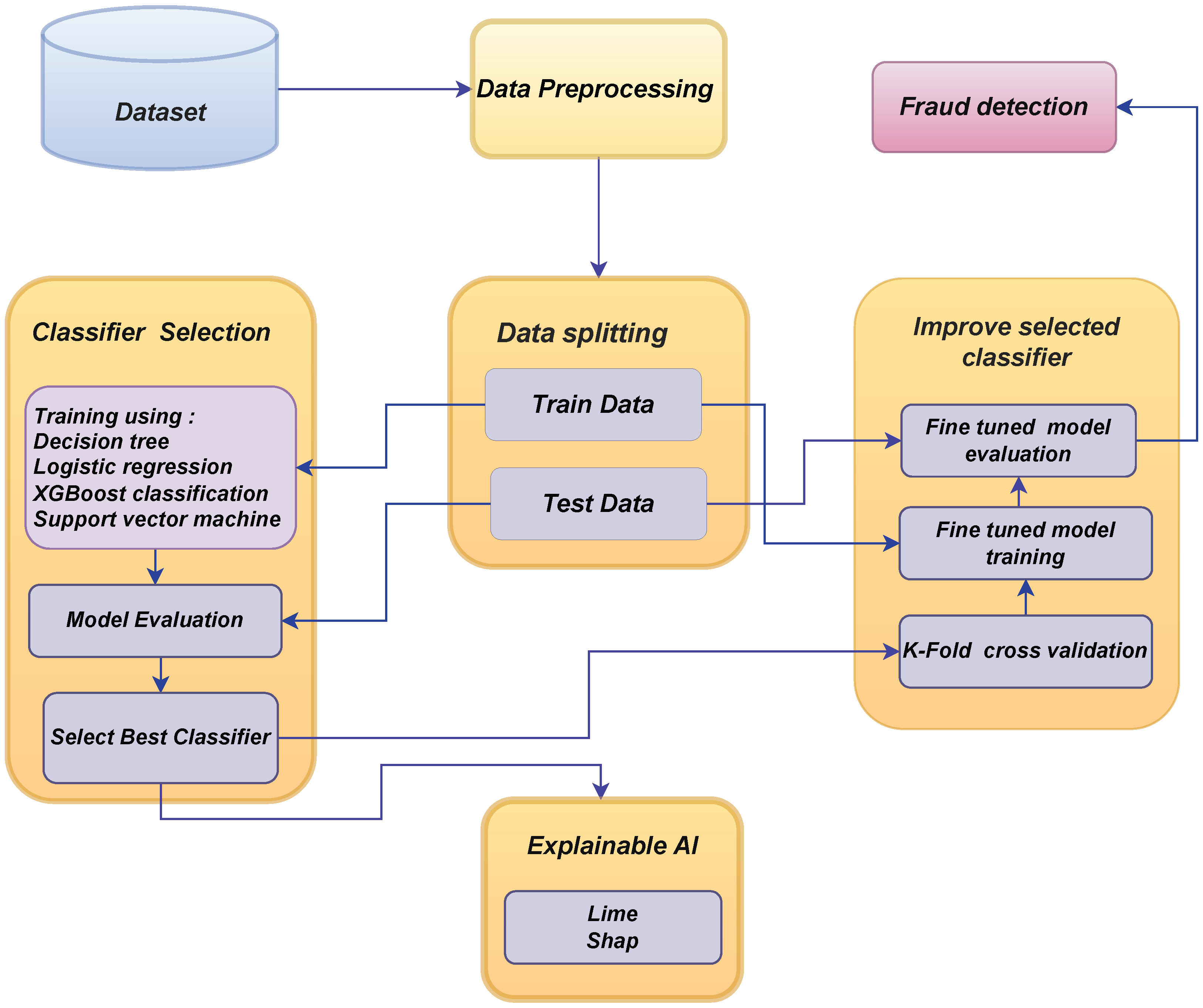
3. Research Methodology of Our Framework
3.1. Dataset Explanation
3.2. Data Preprocessing
3.2.1. SMOTE-Based Data Balancing
| Algorithm 1: SMOTE algorithm |
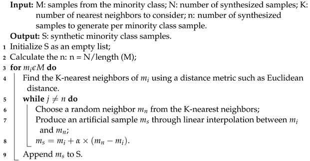 |
3.2.2. LabelEncoder
3.2.3. MinMaxScaler
- = the scaled value of a feature;
- = the feature’s initial value is denoted by this symbol;
- = dataset’s minimum feature value;
- = dataset’s maximum feature value.
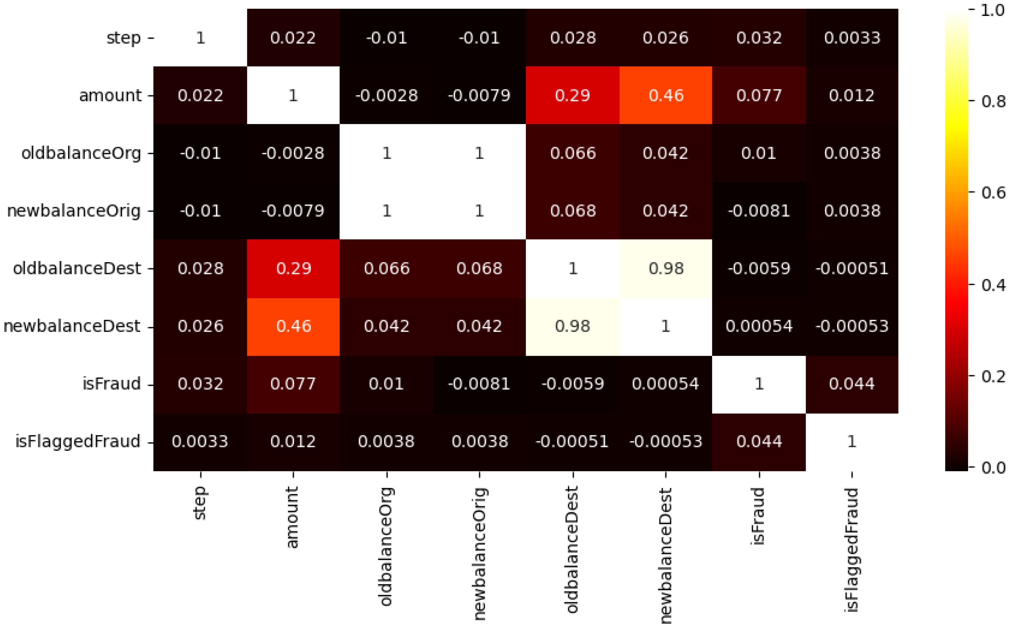
3.3. Correlation Analysis
3.4. Baseline Architectures
Logistic Regression
- y = predicted value;
- x = input value;
- = bias term;
- = the coefficient of the input variable .
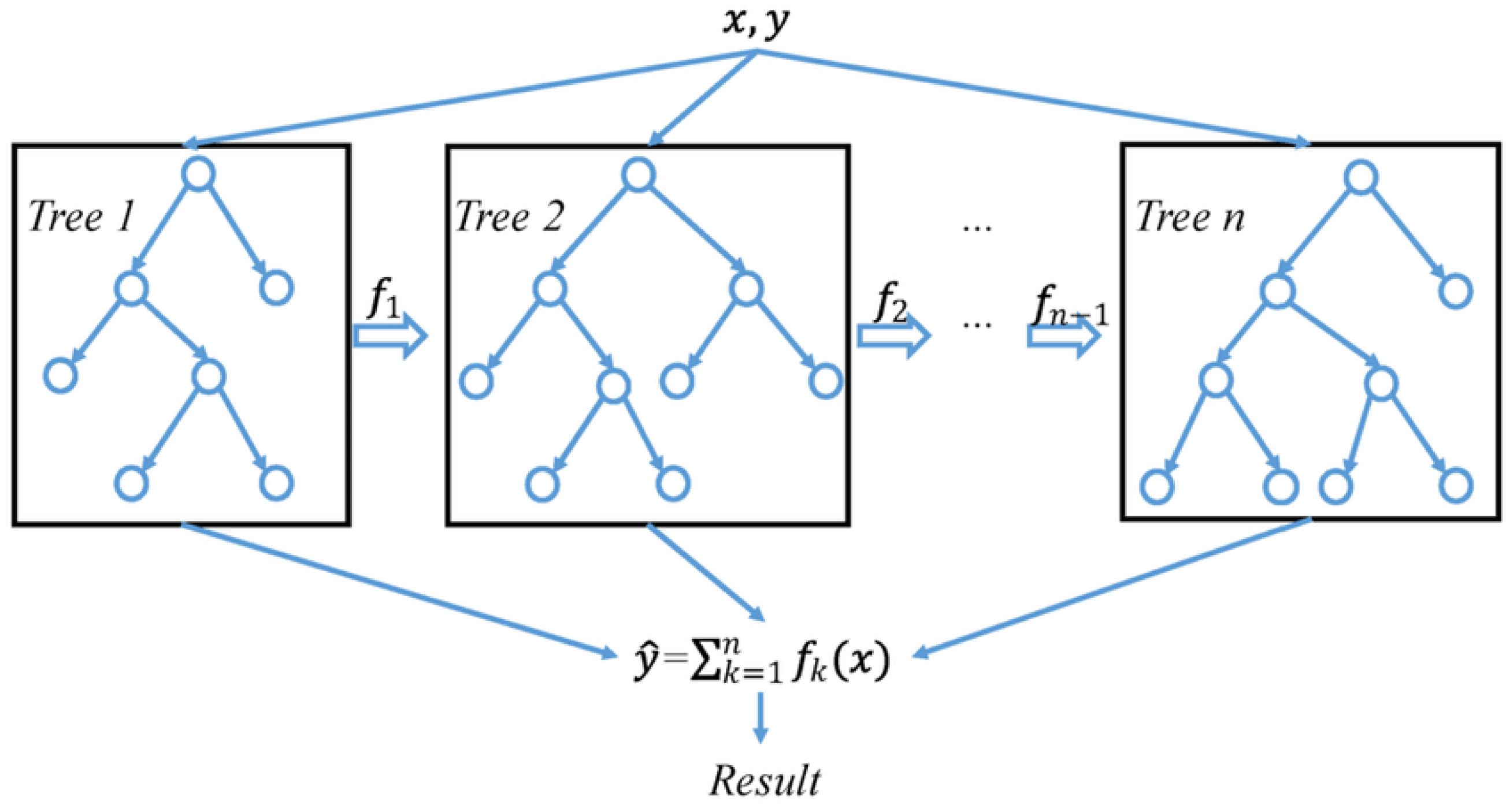
3.5. XGBoost
| Algorithm 2: Detecting fraud with XGboost |
 |
3.6. Decision Tree
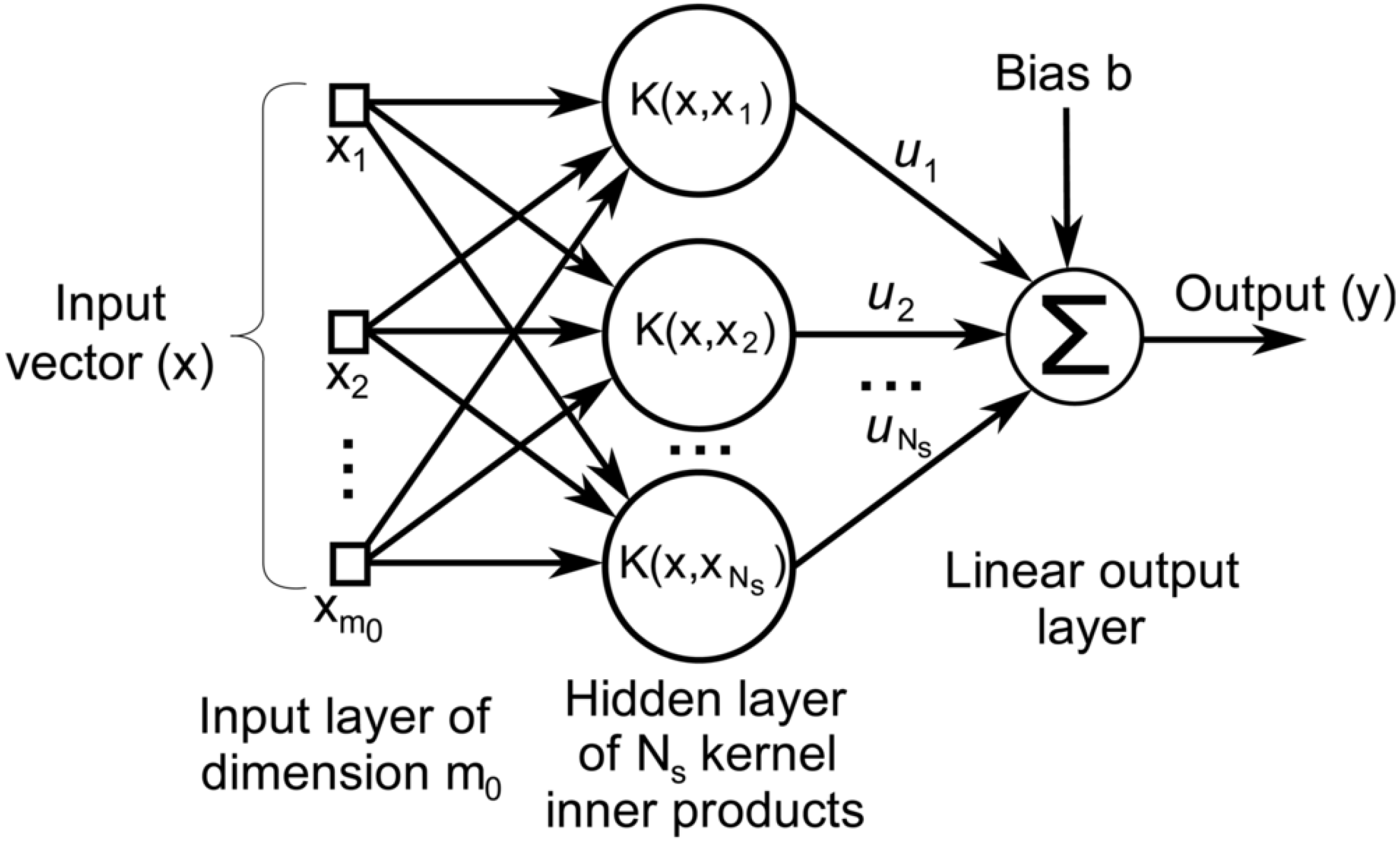
3.7. SVM
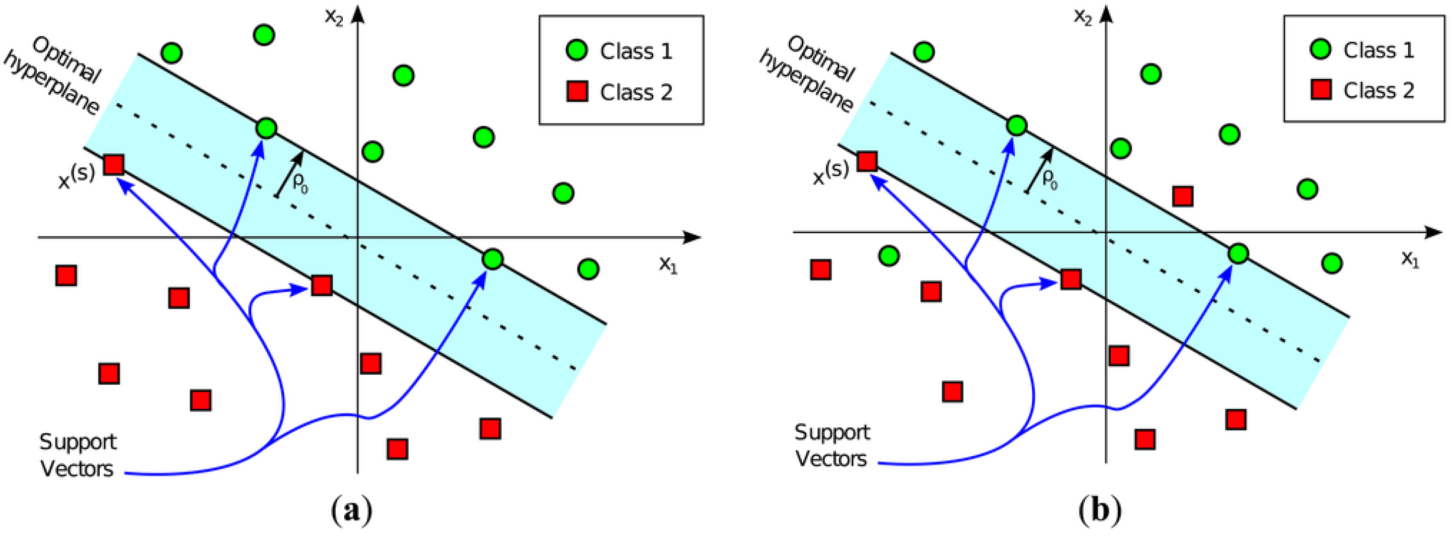
- A hard margin optimality may be employed if the classes in the training dataset can be perfectly separated. Here, the decision boundary of the hyperplane is set such that it is maximally far away from the closest data point in the training set.
- A soft marginal optimality is implemented if completely accurate classification is not desired. Here, the choice of hyperplane is an adjustable compromise between increasing the distance to the next correctly identified training point and decreasing the misclassification rate.
4. Results and Discussion
4.1. Experimental Setup
4.2. Evaluation Measures
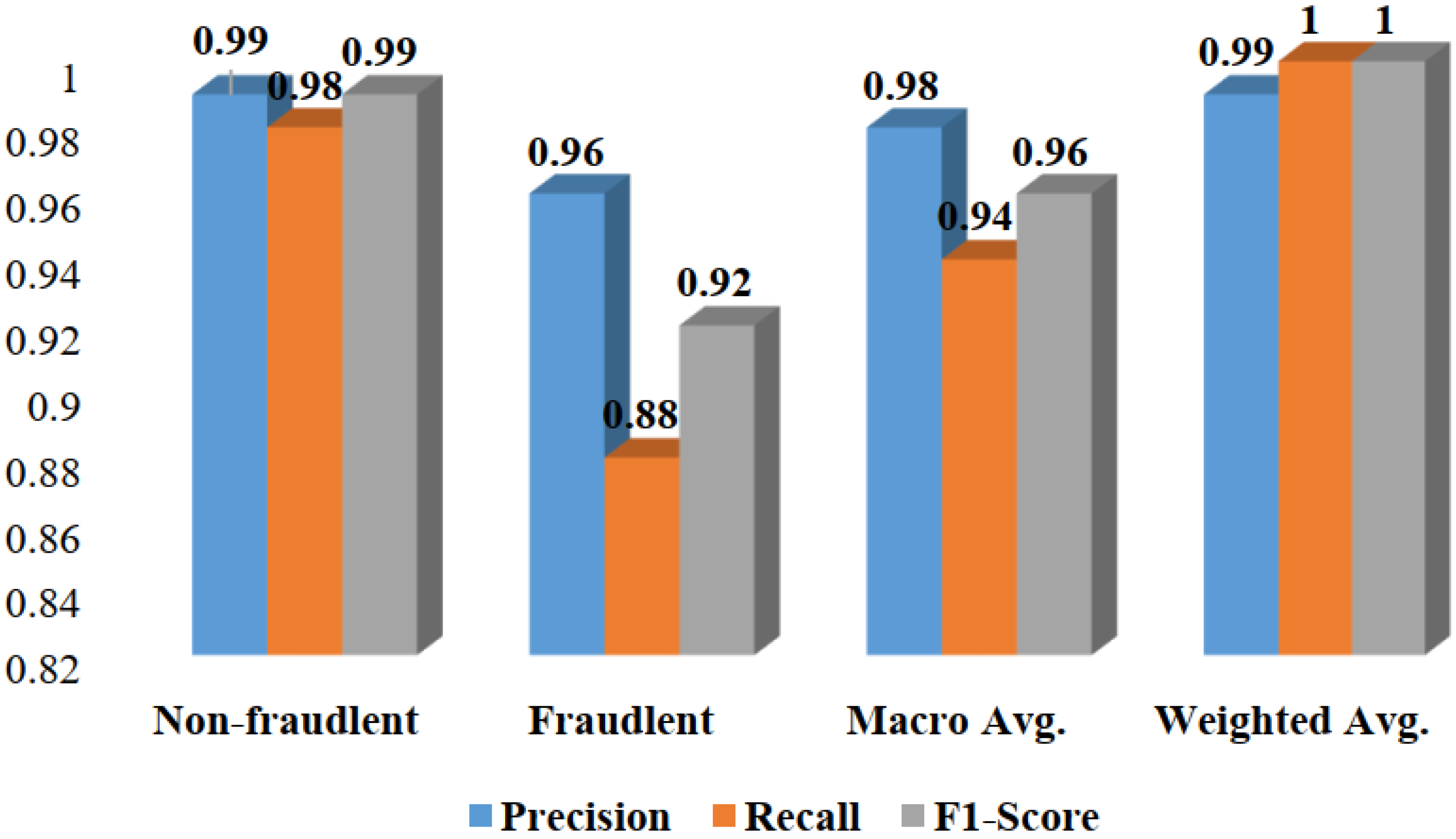
4.3. Result Analysis
4.3.1. K-Fold Cross-Validation
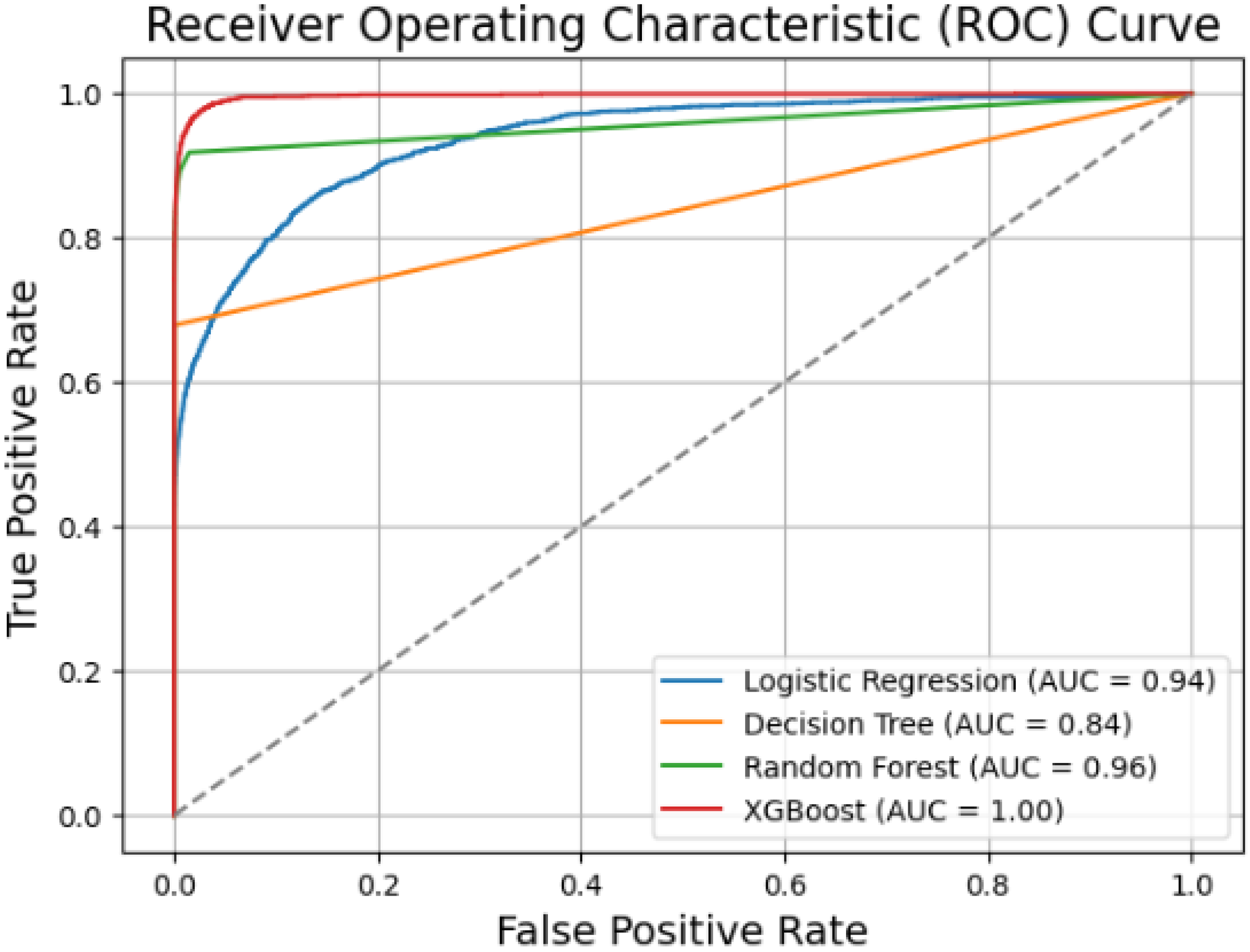
4.3.2. Comparison with Current State-of-the-Art Methods
5. Explainability Analysis
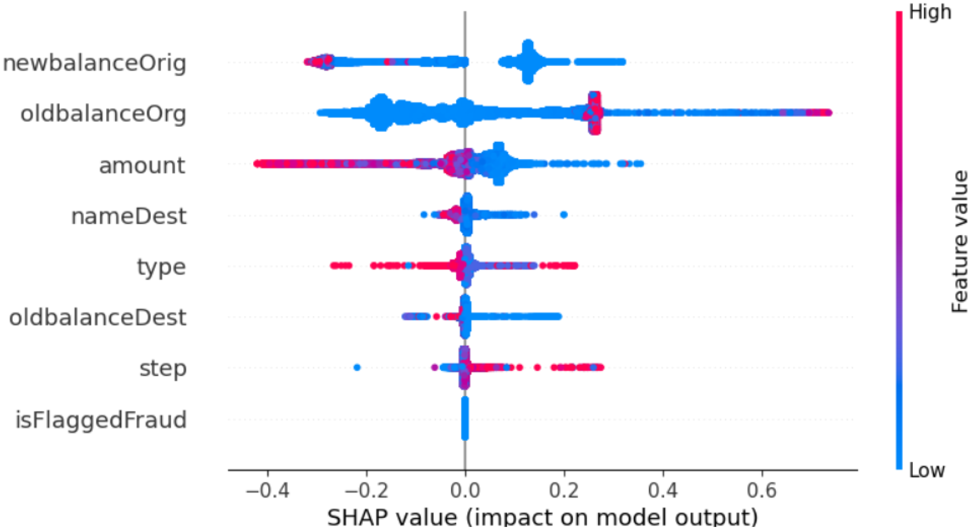
5.1. Model’s Interpretability Using SHAP Analysis
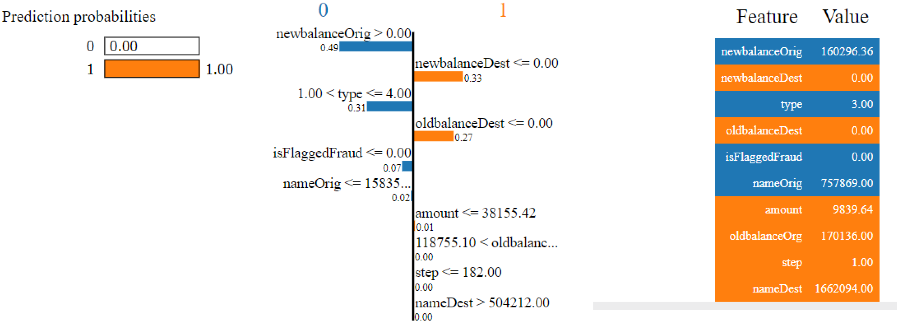
5.2. Model’s Interpretability Using LIME
6. Conclusions and Future Works
Author Contributions
Funding
Institutional Review Board Statement
Informed Consent Statement
Data Availability Statement
Conflicts of Interest
References
- Awoyemi, J.O.; Adetunmbi, A.O.; Oluwadare, S.A. Credit card fraud detection using machine learning techniques: A comparative analysis. In Proceedings of the 2017 International Conference on Computing Networking and Informatics (ICCNI), Lagos, Nigeria, 29–31 October 2017; IEEE: New York, NY, USA, 2017; pp. 1–9. [Google Scholar]
- Mytnyk, B.; Tkachyk, O.; Shakhovska, N.; Fedushko, S.; Syerov, Y. Application of Artificial Intelligence for Fraudulent Banking Operations Recognition. Big Data Cogn. Comput. 2023, 7, 93. [Google Scholar] [CrossRef]
- Yee, O.S.; Sagadevan, S.; Malim, N.H.A.H. Credit card fraud detection using machine learning as data mining technique. J. Telecommun. Electron. Comput. Eng. (JTEC) 2018, 10, 23–27. [Google Scholar]
- Raval, J.; Bhattacharya, P.; Jadav, N.K.; Tanwar, S.; Sharma, G.; Bokoro, P.N.; Elmorsy, M.; Tolba, A.; Raboaca, M.S. RaKShA: A Trusted Explainable LSTM Model to Classify Fraud Patterns on Credit Card Transactions. Mathematics 2023, 11, 1901. [Google Scholar] [CrossRef]
- Irénée, M.; Wang, Y.; Hei, X.; Song, X.; Turiho, J.C.; Nyesheja, E.M. XTS: A Hybrid Framework to Detect DNS-Over-HTTPS Tunnels Based on XGBoost and Cooperative Game Theory. Mathematics 2023, 11, 2372. [Google Scholar] [CrossRef]
- Hasib, K.M.; Tanzim, A.; Shin, J.; Faruk, K.O.; Al Mahmud, J.; Mridha, M. BMNet-5: A novel approach of neural network to classify the genre of Bengali music based on audio features. IEEE Access 2022, 10, 108545–108563. [Google Scholar] [CrossRef]
- Hasib, K.M.; Iqbal, M.; Shah, F.M.; Mahmud, J.A.; Popel, M.H.; Showrov, M.; Hossain, I.; Ahmed, S.; Rahman, O. A survey of methods for managing the classification and solution of data imbalance problem. arXiv 2020, arXiv:2012.11870. [Google Scholar] [CrossRef]
- Maitra, S.; Hossain, T.; Hasib, K.M.; Shishir, F.S. Graph theory for dimensionality reduction: A case study to prognosticate parkinson’s. In Proceedings of the 2020 11th IEEE Annual Information Technology, Electronics and Mobile Communication Conference (IEMCON), Vancouver, BC, Canada, 4–7 November 2020; IEEE: New York, NY, USA, 2020; pp. 134–140. [Google Scholar]
- Jahan, S.; Islam, M.R.; Hasib, K.M.; Naseem, U.; Islam, M.S. Active Learning with an Adaptive Classifier for Inaccessible Big Data Analysis. In Proceedings of the 2021 International Joint Conference on Neural Networks (IJCNN), Shenzhen, China, 18–22 July 2021; IEEE: New York, NY, USA, 2021; pp. 1–7. [Google Scholar]
- Varmedja, D.; Karanovic, M.; Sladojevic, S.; Arsenovic, M.; Anderla, A. Credit card fraud detection-machine learning methods. In Proceedings of the 2019 18th International Symposium INFOTEH-JAHORINA (INFOTEH), Novi Sad, Serbia, 20–22 March 2019; IEEE: New York, NY, USA, 2019; pp. 1–5. [Google Scholar]
- Pech, R. Fraud Detection in Mobile Money Transfer as Binary Classification Problem; Eagle Technilogies Inc Publ: Arlington, VA, USA, 2019; pp. 1–15. [Google Scholar]
- Oza, A. Fraud detection using machine learning. Transfer 2018, 528812, 532909. [Google Scholar]
- Kurshan, E.; Shen, H.; Yu, H. Financial crime & fraud detection using graph computing: Application considerations & outlook. In Proceedings of the 2020 Second International Conference on Transdisciplinary AI (TransAI), Irvine, CA, USA, 21–23 September 2020; IEEE: New York, NY, USA, 2020; pp. 125–130. [Google Scholar]
- Pambudi, B.N.; Hidayah, I.; Fauziati, S. Improving money laundering detection using optimized support vector machine. In Proceedings of the 2019 International Seminar on Research of Information Technology and Intelligent Systems (ISRITI), Yogyakarta, Indonesia, 5–6 December 2019; IEEE: New York, NY, USA, 2019; pp. 273–278. [Google Scholar]
- Zhang, Y.; Trubey, P. Machine learning and sampling scheme: An empirical study of money laundering detection. Comput. Econ. 2019, 54, 1043–1063. [Google Scholar] [CrossRef]
- Raiter, O. Applying supervised machine learning algorithms for fraud detection in anti-money laundering. J. Mod. Issues Bus. Res. 2021, 1, 14–26. [Google Scholar]
- Lopez-Rojas, E.A.; Barneaud, C. Advantages of the PaySim simulator for improving financial fraud controls. In Intelligent Computing: Proceedings of the 2019 Computing Conference, Volume 2; Springer: Berlin/Heidelberg, Germany, 2019; pp. 727–736. [Google Scholar]
- Besenbruch, J. Fraud Detection Using Machine Learning Techniques. Research Paper Business Analytics. 2018. Available online: https://vu-business-analytics.github.io/internship-office/papers/paper-besenbruch.pdf (accessed on 30 April 2024).
- Kuppa, A.; Le-Khac, N.A. Adversarial XAI methods in cybersecurity. IEEE Trans. Inf. Forensics Secur. 2021, 16, 4924–4938. [Google Scholar] [CrossRef]
- Ngai, E.W.; Hu, Y.; Wong, Y.H.; Chen, Y.; Sun, X. The application of data mining techniques in financial fraud detection: A classification framework and an academic review of literature. Decis. Support Syst. 2011, 50, 559–569. [Google Scholar] [CrossRef]
- Saia, R.; Carta, S. Evaluating Credit Card Transactions in the Frequency Domain for a Proactive Fraud Detection Approach; SECRYPT: Berlin, Germany, 2017; pp. 335–342. [Google Scholar]
- Carcillo, F.; Le Borgne, Y.A.; Caelen, O.; Kessaci, Y.; Oblé, F.; Bontempi, G. Combining unsupervised and supervised learning in credit card fraud detection. Inf. Sci. 2021, 557, 317–331. [Google Scholar] [CrossRef]
- Zhao, Z.; Bai, T. Financial Fraud Detection and Prediction in Listed Companies Using SMOTE and Machine Learning Algorithms. Entropy 2022, 24, 1157. [Google Scholar] [CrossRef] [PubMed]
- Nascita, A.; Montieri, A.; Aceto, G.; Ciuonzo, D.; Persico, V.; Pescapé, A. Improving performance, reliability, and feasibility in multimodal multitask traffic classification with XAI. IEEE Trans. Netw. Serv. Manag. 2023, 20, 1267–1289. [Google Scholar] [CrossRef]
- Khatri, S.; Arora, A.; Agrawal, A.P. Supervised machine learning algorithms for credit card fraud detection: A comparison. In Proceedings of the 2020 10th International Conference on Cloud Computing, Data Science & Engineering (Confluence), Noida, India, 29–31 January 2020; IEEE: New York, NY, USA, 2020; pp. 680–683. [Google Scholar]
- Hema, A. Machine Learning methods for Discovering Credit Card Fraud. IRJCS Int. Res. J. Comput. Sci. 2020, III, 1–6. [Google Scholar]
- Kumar, M.S.; Soundarya, V.; Kavitha, S.; Keerthika, E.; Aswini, E. Credit card fraud detection using random forest algorithm. In Proceedings of the 2019 3rd International Conference on Computing and Communications Technologies (ICCCT), Chennai, India, 21–22 February 2019; IEEE: New York, NY, USA, 2019; pp. 149–153. [Google Scholar]
- Seera, M.; Lim, C.P.; Kumar, A.; Dhamotharan, L.; Tan, K.H. An intelligent payment card fraud detection system. Ann. Oper. Res. 2021, 334, 445–467. [Google Scholar] [CrossRef]
- Puh, M.; Brkić, L. Detecting credit card fraud using selected machine learning algorithms. In Proceedings of the 2019 42nd International Convention on Information and Communication Technology, Electronics and Microelectronics (MIPRO), Opatija, Croatia, 20–24 May 2019; IEEE: New York, NY, USA, 2019; pp. 1250–1255. [Google Scholar]
- Lopez-Rojas, E.; Elmir, A.; Axelsson, S. PaySim: A financial mobile money simulator for fraud detection. In Proceedings of the 28th European Modeling and Simulation Symposium, EMSS, Larnaca, Cyprus, 26–28 September 2016; Dime University of Genoa: Genoa, Italy, 2016; pp. 249–255. [Google Scholar]
- Sklearn.Preprocessing.LabelEncoder—scikit-learn.org. Available online: https://scikit-learn.org/stable/modules/generated/sklearn.preprocessing.LabelEncoder.html (accessed on 1 July 2023).
- Sklearn.Preprocessing.MinMaxScaler—scikit-learn.org. Available online: https://scikit-learn.org/stable/modules/generated/sklearn.preprocessing.MinMaxScaler.html (accessed on 1 July 2023).
- Islam, M.T.; Hasib, K.M.; Rahman, M.M.; Tusher, A.N.; Alam, M.S.; Islam, M.R. Convolutional Auto-Encoder and Independent Component Analysis Based Automatic Place Recognition for Moving Robot in Invariant Season Condition. Hum. Centric Intell. Syst. 2022, 3, 13–24. [Google Scholar] [CrossRef]
- Hasnat, F.; Hasan, M.M.; Nasib, A.U.; Adnan, A.; Khanom, N.; Islam, S.M.; Mehedi, M.H.K.; Iqbal, S.; Rasel, A.A. Understanding Sarcasm from Reddit texts using Supervised Algorithms. In Proceedings of the 2022 IEEE 10th Region 10 Humanitarian Technology Conference (R10-HTC), Hyderabad, India, 6–18 September 2022; IEEE: New York, NY, USA, 2022; pp. 1–6. [Google Scholar]
- Hossain, M.S.; Arefin, M.S. Development of an Intelligent Job Recommender System for Freelancers using Client’s Feedback Classification and Association Rule Mining Techniques. J. Softw. 2019, 14, 312–339. [Google Scholar] [CrossRef]
- Jullum, M.; Løland, A.; Huseby, R.B.; Ånonsen, G.; Lorentzen, J. Detecting money laundering transactions with machine learning. J. Money Laund. Control 2020, 23, 173–186. [Google Scholar] [CrossRef]
- Chen, T.; Guestrin, C. Xgboost: A scalable tree boosting system. In Proceedings of the 22nd ACM Sigkdd International Conference on Knowledge Discovery and Data Mining, San Francisco, CA, USA, 13–17 August 2016; pp. 785–794. [Google Scholar]
- Wang, Y.; Pan, Z.; Zheng, J.; Qian, L.; Li, M. A hybrid ensemble method for pulsar candidate classification. Astrophys. Space Sci. 2019, 364, 139. [Google Scholar] [CrossRef]
- Cody, C.; Ford, V.; Siraj, A. Decision tree learning for fraud detection in consumer energy consumption. In Proceedings of the 2015 IEEE 14th International Conference on Machine Learning and Applications (ICMLA), Miami, FL, USA, 9–11 December 2015; IEEE: New York, NY, USA, 2015; pp. 1175–1179. [Google Scholar]
- Javed Mehedi Shamrat, F.; Ranjan, R.; Hasib, K.M.; Yadav, A.; Siddique, A.H. Performance evaluation among id3, c4. 5, and cart decision tree algorithm. In Pervasive Computing and Social Networking: Proceedings of ICPCSN 2021; Springer: Berlin/Heidelberg, Germany, 2022; pp. 127–142. [Google Scholar]
- Nobel, S.N.; Sultana, S.; Tasir, M.A.M.; Rahman, M.S. Next Word Prediction in Bangla Using Hybrid Approach. In Proceedings of the 2023 26th International Conference on Computer and Information Technology (ICCIT), Cox’s Bazar, Bangladesh, 13–15 December 2023; pp. 1–6. [Google Scholar]
- Quinlan, J.R. Induction of decision trees. Mach. Learn. 1986, 1, 81–106. [Google Scholar] [CrossRef]
- Salzberg, S.L. C4. 5: Programs for Machine Learning; Quinlan, J.R., Ed.; Morgan Kaufmann Publishers, Inc.: San Francisco, CA, USA, 1993. [Google Scholar]
- Cortes, C.; Vapnik, V. Support-vector networks. Mach. Learn. 1995, 20, 273–297. [Google Scholar] [CrossRef]
- Salehi, A.; Ghazanfari, M.; Fathian, M. Data mining techniques for anti money laundering. Int. J. Appl. Eng. Res. 2017, 12, 10084–10094. [Google Scholar]
- Ruiz-Gonzalez, R.; Gomez-Gil, J.; Gomez-Gil, F.J.; Martínez-Martínez, V. An SVM-based classifier for estimating the state of various rotating components in agro-industrial machinery with a vibration signal acquired from a single point on the machine chassis. Sensors 2014, 14, 20713–20735. [Google Scholar] [CrossRef] [PubMed]
- Li, D.; Jiang, M.R.; Li, M.W.; Hong, W.C.; Xu, R.Z. A floating offshore platform motion forecasting approach based on EEMD hybrid ConvLSTM and chaotic quantum ALO. Appl. Soft Comput. 2023, 144, 110487. [Google Scholar] [CrossRef]
- Hossen, R.; Whaiduzzaman, M.; Uddin, M.N.; Islam, M.J.; Faruqui, N.; Barros, A.; Sookhak, M.; Mahi, M.J.N. Bdps: An efficient spark-based big data processing scheme for cloud fog-iot orchestration. Information 2021, 12, 517. [Google Scholar] [CrossRef]
- Whaiduzzaman, M.; Sakib, A.; Khan, N.J.; Chaki, S.; Shahrier, L.; Ghosh, S.; Rahman, M.S.; Mahi, M.J.N.; Barros, A.; Fidge, C.; et al. Concept to Reality: An Integrated Approach to Testing Software User Interfaces. Appl. Sci. 2023, 13, 11997. [Google Scholar] [CrossRef]
- Achar, S.; Faruqui, N.; Whaiduzzaman, M.; Awajan, A.; Alazab, M. Cyber-physical system security based on human activity recognition through IoT cloud computing. Electronics 2023, 12, 1892. [Google Scholar] [CrossRef]
- Ekanayake, I.; Meddage, D.; Rathnayake, U. A novel approach to explain the black-box nature of machine learning in compressive strength predictions of concrete using Shapley additive explanations (SHAP). Case Stud. Constr. Mater. 2022, 16, e01059. [Google Scholar] [CrossRef]
- Ahmed, S.; Nobel, S.N.; Ullah, O. An effective deep CNN model for multiclass brain tumor detection using MRI images and SHAP explainability. In Proceedings of the 2023 International Conference on Electrical, Computer and Communication Engineering (ECCE), Chittagong, Bangladesh, 23–25 February 2023; pp. 1–6. [Google Scholar]
- Khedkar, S.; Subramanian, V.; Shinde, G.; Gandhi, P. Explainable AI in healthcare. In Proceedings of the 2nd International Conference on Advances in Science & Technology (ICAST), Mumbai, India, 8–9 April 2019. [Google Scholar]


| Methods | Contribution | Limitation |
|---|---|---|
| RF, NB, MLP [10] | Assessed the three ML algorithms’ credit card fraudulent transactions detection | The short-term nature of the dataset may reduce the generalization ability. |
| Hybrid Model [22] | A novel hybrid framework that seamlessly integrates supervised and unsupervised methodologies to enhance the accuracy of fraud detection. | |
| Logistic Regression and XGBoost [23] | An ensemble machine learning framework for detecting fraudulent credit card transactions leveraging an imbalanced dataset. | Lacks an explanation of the feature selection process. |
| KNN, DT, LR, RF, and NB [25] | Used a severely imbalanced dataset to evaluate ML algorithms for detecting fraudulent transactions with credit cards. | Poor classification performence. |
| RF, LR, and Category Boosting (CatBoost) [26] | The performance of RF, LR, and Category Boosting (CatBoost) is evaluated to obtain the most efficient model for evaluating the ECCFD dataset. | Did not tackle the class imbalance issue. |
| NB, LR, and KNN [1] | The imbalanced dataset was addressed through hybrid sampling. | Poor classification performance of LR. Also, did not implement the feature selection method. |
| GA-RF, GA-ANN, GBT, and GA-DT [28] | Applied Genetic Algorithms (GA) for feature selection and aggregation, along with multiple machine learning methods, to evaluate the approach’s effectiveness. | Consumer transactional aspects must be assessed using data from several regions, although this study concentrates only on Malaysian financial transactions. |
| Data Splitting | Original | SMOTE | RandomUnderSampler |
|---|---|---|---|
| Training dataset | 5090096 | 10167051 | 13140 |
| Test dataset | 1272524 | 2541763 | 3286 |
| Model | Details of Parameters |
|---|---|
| Logistic Regression | random state = 42. |
| XGBoost | n_estimators = 341 |
| max_depth = 7, | |
| subsample = 0.9, | |
| learning rate = 0.001, | |
| = 0.5. | |
| Decision Tree | min samples split = 69 |
| cirterion = entropy | |
| splitter = 42 | |
| SVM | kernel = linear, |
| C = 1.0 |
| Model | Precision | Recall | F1-Score | Accuracy |
|---|---|---|---|---|
| Logistic Regression | 0.92 | 0.86 | 0.89 | 98.99% |
| XGBClassifier | 0.96 | 0.88 | 0.92 | 99.88% |
| Decision Tree | 0.87 | 0.85 | 0.86 | 98.96% |
| SVM | 0.64 | 0.36 | 0.48 | 96.91% |
| Model | SMOTE | Normal | Undersampling |
|---|---|---|---|
| Logistic Regression | 98.99% | 96.89% | 81.71% |
| XGBClassifier | 99.88% | 95.97% | 97.41% |
| Decision Tree | 98.96% | 97.87% | 96.74% |
| SVM | 96.91% | 92.74% | 88.89% |
| Value of K | Train_acc (%) | Valid_acc (%) |
|---|---|---|
| Fold = 1 | 99.991 | 99.973 |
| Fold = 2 | 99.991 | 99.952 |
| Fold = 3 | 99.991 | 99.984 |
| Fold = 4 | 99.991 | 99.983 |
| Fold = 5 | 99.991 | 99.982 |
| Fold = 6 | 99.992 | 99.979 |
| Fold = 7 | 99.991 | 99.980 |
| Fold = 8 | 99.992 | 99.984 |
| Fold = 9 | 99.991 | 99.980 |
| Fold = 10 | 99.993 | 99.984 |
| Reference | Dataset | Accuracy (%) |
|---|---|---|
| RF = 99.96, | ||
| [10] | Credit card fraud detection | NB = 99.23 |
| MLP = 99.93 | ||
| [23] | Transaction records: 18,060 | Logistic Regression + XGBOOST = 98.523 |
| Credit card transactions | Logistic Regression = 99.88 | |
| [26] | conducted by European cardholders. | Random Forest = 99.95 |
| CatBoost = 99.93 | ||
| NB = 97.92 | ||
| [1] | Credit card transactions | KNN= 97.69 |
| Total transaction records: 284,807 | LR = 54.86 | |
| [28] | Statlog (Australian Credit) | Gradient Boosted Trees (GBT) = 96.7 |
| Proposed Method | Synthetic Financial Datasets | 99.88 |
Disclaimer/Publisher’s Note: The statements, opinions and data contained in all publications are solely those of the individual author(s) and contributor(s) and not of MDPI and/or the editor(s). MDPI and/or the editor(s) disclaim responsibility for any injury to people or property resulting from any ideas, methods, instructions or products referred to in the content. |
© 2024 by the authors. Licensee MDPI, Basel, Switzerland. This article is an open access article distributed under the terms and conditions of the Creative Commons Attribution (CC BY) license (https://creativecommons.org/licenses/by/4.0/).
Share and Cite
Nobel, S.M.N.; Sultana, S.; Singha, S.P.; Chaki, S.; Mahi, M.J.N.; Jan, T.; Barros, A.; Whaiduzzaman, M. Unmasking Banking Fraud: Unleashing the Power of Machine Learning and Explainable AI (XAI) on Imbalanced Data. Information 2024, 15, 298. https://doi.org/10.3390/info15060298
Nobel SMN, Sultana S, Singha SP, Chaki S, Mahi MJN, Jan T, Barros A, Whaiduzzaman M. Unmasking Banking Fraud: Unleashing the Power of Machine Learning and Explainable AI (XAI) on Imbalanced Data. Information. 2024; 15(6):298. https://doi.org/10.3390/info15060298
Chicago/Turabian StyleNobel, S. M. Nuruzzaman, Shirin Sultana, Sondip Poul Singha, Sudipto Chaki, Md. Julkar Nayeen Mahi, Tony Jan, Alistair Barros, and Md Whaiduzzaman. 2024. "Unmasking Banking Fraud: Unleashing the Power of Machine Learning and Explainable AI (XAI) on Imbalanced Data" Information 15, no. 6: 298. https://doi.org/10.3390/info15060298
APA StyleNobel, S. M. N., Sultana, S., Singha, S. P., Chaki, S., Mahi, M. J. N., Jan, T., Barros, A., & Whaiduzzaman, M. (2024). Unmasking Banking Fraud: Unleashing the Power of Machine Learning and Explainable AI (XAI) on Imbalanced Data. Information, 15(6), 298. https://doi.org/10.3390/info15060298