An Efficient Ensemble Approach for Brain Tumors Classification Using Magnetic Resonance Imaging

Abstract

Tumors in the brain can be life-threatening, making early and precise detection crucial for effective treatment and improved patient outcomes. Deep learning (DL) techniques have shown significant potential in automating the early diagnosis of brain tumors by analyzing magnetic resonance imaging (MRI), offering a more efficient and accurate approach to classification. Deep convolutional neural networks (DCNNs), which are a sub-field of DL, have the potential to analyze rapidly and accurately MRI data and, as such, assist human radiologists, facilitating quicker diagnoses and earlier treatment initiation. This study presents an ensemble of three high-performing DCNN models, i.e., DenseNet169, EfficientNetB0, and ResNet50, for accurate classification of brain tumors and non-tumor MRI samples. Our proposed ensemble model demonstrates significant improvements over various evaluation parameters compared to individual state-of-the-art (SOTA) DCNN models. We implemented ten SOTA DCNN models, i.e., EfficientNetB0, ResNet50, DenseNet169, DenseNet121, SqueezeNet, ResNet34, ResNet18, VGG16, VGG19, and LeNet5, and provided a detailed performance comparison. We evaluated these models using two learning rates (LRs) of 0.001 and 0.0001 and two batch sizes (BSs) of 64 and 128 and identified the optimal hyperparameters for each model. Our findings indicate that the ensemble approach outperforms individual models, having 92% accuracy, 90% precision, 92% recall, and an F1 score of 91% at a 64 BS and 0.0001 LR. This study not only highlights the superior performance of the ensemble technique but also offers a comprehensive comparison with the latest research.

1. Introduction

Brain tumors are a serious medical condition with potentially life-threatening consequences, affecting the central nervous system (CNS) by disrupting vital functions in the brain and spinal cord. These tumors can be classified into several types, with meningioma, glioma, and pituitary adenomas being the most common. Understanding and accurately diagnosing these tumors is critical for ensuring patients receive timely and appropriate treatment [1].

Meningiomas arise from the meninges, the protective membranes that cover the brain and spinal cord. While they are typically benign, certain cases can develop into malignant forms, depending on the tumor size and growth rate. Gliomas, on the other hand, develop from glial cells, which play a supportive role for neurons. Gliomas represent the largest group of primary brain tumors and vary significantly in terms of aggressiveness and biological characteristics. They can range from low-grade, slow-growing tumors to highly malignant forms like glioblastoma. The third type, pituitary adenomas, are benign tumors that form in the pituitary gland, a small but critical gland located at the base of the brain. These tumors can disrupt hormonal functions and, depending on their size, may cause pressure on surrounding brain structures. Although mostly benign, pituitary adenomas constitute approximately 10% of all intracranial tumors [2].

Diagnosing and classifying these brain tumors accurately is a complex task due to the overlapping features in medical imaging, particularly MRI scans. Conventional methods often rely on radiologists’ expertise, which can be subjective and time-consuming. Artificial intelligence (AI) is nowadays applicable in various domains for disease detection, i.e., early detection and classification of different diseases in humans [3,4,5]. Similarly, AI, especially deep learning (DL), can significantly improve the early classification of brain tumors using magnetic resonance imaging (MRI). The DL technique can analyze large amounts of MRI data much faster than humans. This allows for a quicker diagnosis, which is crucial for starting treatment early. DL techniques, especially deep convolution neural networks (DCNNs), can detect abnormalities in MRIs more accurately and quickly than radiologists [6]. This high level of accuracy can lead to earlier detection of brain tumors. DCNN models can be trained on large datasets to differentiate between different types of brain tumors. This ability helps identify the specific type of tumor, which is essential for choosing the right treatment plan. The DCNN algorithms are helpful for brain tumor classification. It can reduce the workload on radiologists, allowing them to focus on more complex cases. This efficiency can lead to better overall healthcare outcomes for patients [7].

Our study focuses on the influence of DCNN-based models with varied hyperparameters to assess their performance using MRI-based brain tumor classification. After evaluating the individual performance of several DCNN architectures, we identified three top-performing models: DenseNet169, EfficientNetB0, and ResNet50. We implemented an ensemble approach to capitalize on the strengths of each model. This approach combines the outputs of these three high-performing DCNNs to create a more robust and accurate classification system. This ensemble technique harnesses the unique features and learning capabilities of each model, potentially leading to improved overall performance in distinguishing between different tumors and non-tumor MRI samples. The contribution of our study is discussed in later sections; however, a brief overview is as below:

• Our proposed ensemble model provides prominent results. We observed a significant improvement in evaluation parameters, especially improved classification accuracy using our approach.
• This study provides the implementation of ten SOTA DCNN models, i.e., EfficientNetB0, ResNet50, DenseNet169, DenseNet121, SqueezeNet, ResNet34, ResNet18, VGG16, VGG19, and LeNet, and a detailed performance comparison of them. We also observe better results when we compare our proposed ensemble technique’s with SOTA DCNN models.
• We compare results using two LRs of 0.001 and 0.0001 and two BS of 64 and 128. We highlight the best LR and BS for the respective model.

2. Related Work

Several approaches are available in the literature to detect brain tumors. These approaches include basic machine learning algorithms, DL approaches, and a hybrid of both. Therefore, this section presents the overview and analysis of the related research to detect brain tumors using MRI scans.

Khairandish et al. [8] used MRI scans for the classification of brain tumors. Their methodology involved CNN for feature extraction and support vector machines (SVMs) to learn the features and classify them. The model could analyze brain images using CNN and hybrid SVM as a supervised learning approach to categorize normal and cancerous scans. The input images were preprocessed as resized, and then normalization was carried out. Considerable features from the preprocessed image were extracted using the maximally stable extremal regions and the segmentation method based on a threshold. To perform a classification of brain MRI images, the segmented features were labeled and trained through hybrid CNN and SVM algorithms. The researcher used the BRATS 2015 dataset to validate their approach. The hierarchical DL model was developed by Khan et al. [9], in which they proposed a brain tumor classifying model. Three steps made up their proposed approach included data generation, data interpretation, and data use. The MRI scans were obtained first from internet of medical things (IoMT) devices and transferred to the data acquisition layer. Assam et al. [10] proposed a unique method. The preprocessing of MRI images involved applying a median filter, and they then used discrete wavelet transform (DVT) and color moments to extract features. Those features were utilized to create feed-forward artificial neural networks (FF-ANNs) for the classification of brain MRI scans using random forest (RF) and residual sum of squares (RSSs) classifiers. A self-collected dataset of 70 T2-weighted images from Harvard Medical School was used to evaluate their methodology.

Noreen et al. [11] used DCNN-based pre-trained models, i.e., Inception-V3 and DensNet201, to detect brain tumors. The authors used four dense blocks in DensNet201 and eleven inception modules in Inception-V3, where the number of convolution layer features varied depending on the architecture to extract features and end with a softmax classification layer. Their approach incorporated both local and global multi-level feature extraction and concatenation of the resulting features. The data for testing the model under consideration was comprised of 3064 T1-weighted contrast MRI images. Ghassemi et al. [12] proposed a framework consisting of training a DCNN model as the discriminator in the GAN. Its task was to distinguish between fraudulent and genuine MRI scans synthesized by the generative model. Therefore, the discriminator assessed and quantified the features of MRI scans and identified the intricate structure of MRI scans. It was a classification model for brain tumors that was fine-tuned through training of the pre-trained CNN on the original dataset. The final fully connected layer of the GAN discriminator was replaced by the seven neuron SoftMax layer for classification. The author loaded the preprocessed image by rotating and mirroring it to boost the training data through data augmentation. It was applied to T1 contrast-enhanced (CE) MRI images and whole brain volume MR images, 3064. Musallam et al. [13] also proposed a framework involving three stages, i.e., preprocessing such as erasing ambiguous objects from the MRI images, noise reduction on the MRI scans, and online histogram equalization to boost the performance of the MRI images. To diagnose the brain tumor, samples of MRIs corresponding to different types of tumors were used to train a DCNN model. The Navoneel brain tumor dataset, which includes both T1 and T2 MRI images, and Sartaj brain MRI images were used to validate their method.

Ismael et al. [14] modified the ResNet50 DL model for classifying brain tumors through the inclusion of three neurons in a layer and establishing a fully connected layer. The researchers augmented their dataset by performing flipping, rotation, shift, scale, whitening, clipping, and brightness. For the assessment, the subjects consisted of 3064 T1-weighted CE MRI images publicly available for brain tumors. Sekhar et al. [15] modified the existing DL model, i.e., GoogleNet, for extracting features from MRI images in combination with SVM and K-NN classifiers. The researchers used two datasets from the Harvard medical archives and the CE-MRI Figshare repository. Their method produced the best classification accuracy when used with the Figshare dataset for 3-class tumor classification and the Harvard Medical Archives for 4-class tumor classification. Compared to the existing models, their proposed approach showed better results.

Irmak et al. [16] proposed a multi-class classification approach using three fully CNN models connected to classify MRI images of brain tumors, followed by a Softmax classifier. Their study involved 3 CNN models: The Model-I CNN model classifier was used for distinguishing brain tumors: brain tumors classified as glioma, meningioma, pituitary, normal, or metastatic using the Model-II CNN classifier; and glioma brain tumors classified as Class II, Class III, and Class IV using the Model-III CNN classifier. A grid search optimizer was used to find optimal hyperparameters for each CNN model.

Table 1. Comprehensive overview of the literature.

Reference	Dataset	Technique Used	Total Scans	Classes	Advantages	Limitations
[8], Khairandish et al.	BRATS’15	Hybrid CNN for feature extraction and SVM for classification	64 LGG 220 HGG MRIs	Normal and tumor	Combines strengths of CNN for feature extraction and SVM for classification; good accuracy on BRATS’15 dataset	Limited to normal and tumor classification only
[9], Khan et al.	Public	Hierarchical DL model	3264	Normal, Meningioma, Pituitary and Glioma,	Hierarchical approach allows for better multi-class tumor classification	Limited description of the exact performance; needs further evaluation on large datasets
[10], Assam et al.	Self-collected acquired from Harvard Medical College (T2 weighted scans)	Median filter, DWT, color moments for feature extraction, FF-ANN, RF, RSS classifiersPre-trained DCNN (InceptionV3, DenseNet201), multi-level feature extraction and concatenation	25 Normal 45 Tumors scans	Normal and tumor	Combination of feature extraction techniques improves classification performance	Small dataset (self-collected, 70 samples); limited generalization capability
[11], Noreen et al.	3064 T1-CE MRI scans	Pre-trained DCNN (InceptionV3, DenseNet201), multi-level feature extraction and concatenation	3064	Glioma, Meningioma, and Pituitary	Pre-trained models reduce the need for large datasets, multi-level feature extraction enhances classification	Lacks of novality and better performance, exploration of lightweight models
[12], Ghassemi et al.	(1) 3064 T1-CE MRI scans (2) Whole brain MRI scans consisting of 373 longitudinal scans via 150 subjects	DCNN as a discriminator in GAN, data augmentation via image transformations	(1) 3064 (2) 156	Pituitary, Meningioma and, Glioma.	GAN enhances robustness by distinguishing genuine/fake MRI scans; data augmentation improves model performance	GAN training can be unstable; limited evaluation on more diverse datasets
[13], Musallam et al.	(1) Sartaj brain MRI dataset (2) Navoneel brain tumor MRI dataset that has two kinds of MRI	DCNN with pre-processing (noise reduction, histogram equalization)	(1) 3394 (2) 3394	Glioma, Meningioma, and Pituitary	Pre-processing improves MRI scan quality; robust validation on different tumor types	Focused on specific MRI types (T1 and T2); lacks broader generalization on unseen datasets
[14], Ismael et al.	Public	Modified ResNet50 with data augmentation	3064	Meningioma, Glioma, and Pituitary	ResNet50 provides good accuracy; data augmentation helps improve model generalization	Their approach may not perform well on smaller datasets
[15], Sekhar et al.	FigShare CE-MRI dataset	Modified GoogleNet with SVM and K-NN classifiers	3064	Glioma, Meningioma, and Pituitary	Combination of GoogleNet and traditional classifiers yields high classification accuracy	Needs comparison with more advanced deep learning models; computationally expensive
[16], Irmak et al.	(1) RIDER (2) REMBRANDT (3) TCGA-LGG	Multi-class classification with CNN and grid search for hyperparameters	(1) 70,220 RIDER (2) 110,020 REMBRANDT (3) 241,183 TCGA-LGG	Model I: Tumor and non-tumor; Model II: Glioma, pituitary, meningioma, metastatic, and normal; Model III: Different grades of glioma tumors	Use of grid search optimizes hyperparameters; CNN models for multi-level tumor classification	Computational complexity increases with multiple CNN models

summarizes the studies provided in paper to classify the brain tumors using machine learning, deep learning, and hybrid approaches, with other details. Khairandish et al. and Khan et al. utilized different models, including hybrid approaches and hierarchical classifiers, on datasets ranging from 220 to 3264 MRI scans to distinguish between normal and tumor tissues. Assam et al. used several models on a smaller dataset of 70 scans, while Noreen et al. and Ghassemi et al. used advanced DL models like InceptionV3 and DCNN on larger datasets of over 3000 scans to identify specific tumor types. Musallam et al. and Ismael et al. used DCNN and ResNet50 on datasets of similar size to classify glioma, meningioma, and pituitary tumors. Sekhar et al. combined GoogLeNet with SVM or KNN on 3064 scans. Whereas Irmak et al. analyzed extensive datasets with CNN models to classify various tumor types and grades.

The remaining sections of the study include methodology with details in Section 3, results comparison and their discussion in Section 4, and conclusion with possible future direction in Section 5.

3. Materials and Methods

Deep learning-based DCNN models enhance the precision of diagnoses, aiding clinicians in delivering targeted treatments. Similarly, Figure 1 illustrates a brain tumor classification workflow using MRI data and an ensemble of deep learning (DL) models. The process begins by splitting the dataset into training and validation sets, followed by preprocessing steps such as encoding, resizing, and normalization. Three pre-trained deep CNN models, i.e., DenseNet169, EfficientNetB0, and ResNet50, are then employed, with their predictions combined through ensemble majority voting. This method classifies MRI scans into four categories: no tumor, glioma, meningioma, or pituitary tumor. The final stage involves analyzing the model performance using training and validation accuracy.

3.1. Dataset Description

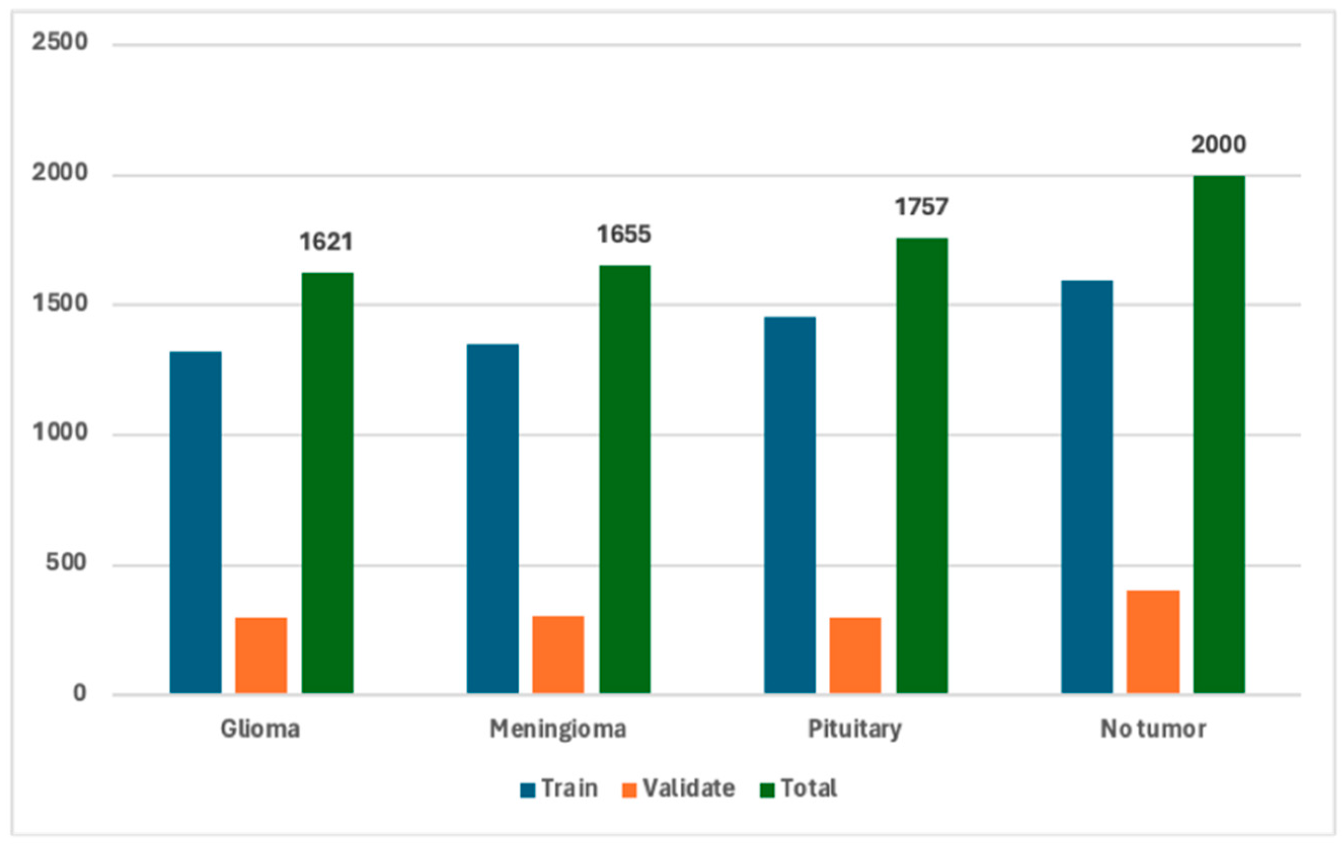
The publicly available dataset from Kaggle [17] has been used in this study and has four classes, i.e., pituitary, glioma, meningioma, and non-tumor samples. Figure 2 shows the MRI samples of each class available in the dataset. The dataset is gathered from three public repositories, i.e., non-tumor samples from the BRATS repository, gliomas samples from the FigShare repository, and meningioma and pituitary samples from the Sartaj dataset. The samples from BraTS images were captured using multiple imaging modalities, including fluid-attenuated inversion recovery (FLAIR), T2-weighted, and T1-weighted with contrast enhanced. The FigShare and Sartaj datasets consist of T1-weighted contrast-enhanced images. The original image resolution is 512 × 512 × 3 for the entire dataset. There are a total of 5722 scans for training, distributed as 1321 gliomas, 1349 meningiomas, 1457 pituitary, and 1595 no tumor. Similarly, there are 1311 scans for validation, with 300 glioma, 306 meningioma, 300 pituitary, and 405 no tumors, as shown in

Table 2. Dataset distribution into training and validation sets.

Class	Train	Validate	Total	Class Label
Glioma	1321	300	1621	“0”
Meningioma	1349	306	1655	“1”
Pituitary	1457	300	1757	“2”
No tumor	1595	405	2000	“3”
Total	5722	1311	7033

. The dataset is considered nearly balanced for different tumor types and non-tumor cases. The label (also known as encoding) against each class is also shown in the table. Figure 3 shows the distribution of the dataset for each class, i.e., 1621 glioma, 1655 meningioma, 1757 pituitary, and 2000 no tumor MRI samples.

3.2. Dataset Preprocessing

Preprocessing is an important step in deep learning while dealing with image data. The vital data preprocessing techniques include resizing and normalization of input data to maintain homogeneity in the size of the feature vectors and scaling of pixel values, which is beneficial to train faster and more efficiently. In our study, the input MRI scans are resized to a target size of 224 × 224 × 3 pixels, and the pixel values are normalized by rescaling them to the range [0,1].

Here x is the pixel value and μ is the mean pixel value in an image. Similarly, σ represents the standard deviation of all pixel values. This normalization helps the model learn more effectively by standardizing the input data.

3.3. Proposed Ensemble of DL DCNN Models

The proposed ensemble consists of three state-of-the-art DCNN models, i.e., ResNet50, DenseNet169, and EfficientNetB0. Each model has unique strengths in extracting hierarchical features from images. The rationale behind using an ensemble of these models is based on the principle that different architectures capture distinct feature representations at varying scales and complexities, which, when combined, can provide a more robust and generalized model. By integrating their outputs, we aim to achieve better classification performance than any single model alone [18].

We focus on classifying MRI images into four distinct classes, i.e., three tumor types and one non-tumor class. The ensemble method aggregates the complementary strengths of these models to improve classification accuracy and reduce generalization error.

3.3.1. Model Architecture

Each of the three models is initialized with pre-trained weights from ImageNet, which allows leveraging transfer learning. The top classification layers from each model are removed, and the remaining network is used as a feature extractor. This means we only retain the convolutional and pooling layers, which are effective in learning spatial hierarchies of features from images. The input image dimensions for all models are standardized to 224 × 224 × 3 (height, width, channels). Here channels refer to T1-weighted, T2-weighted, and FLAIR.

Let $X\in {\mathbb{R}}^{224\times 224\times 3}$ represent the input MRI image. For each model $M_k$ where $k\in \{\mathrm{1,2},3\}$, the model processes $X$ and produces a feature map $F_k$.

$$F_k=M_k\left(X\right)$$

(1)

Here, $F_k\in {\mathbb{R}}^{H_k\times W_k\times D_k}$ where $H_k,W_k$, and $D_k$ represent the height, width, and depth (number of feature channels) of the feature map generated by the model $M_k$.

3.3.2. Global Average Pooling (GAP)

To reduce the dimensionality of each feature map while retaining important information, we apply a GAP layer on each feature map $F_k$. The GAP layer computes the average value across the spatial dimensions (height and width) for each feature channel, resulting in a vector of size $D_k$, where $D_k$ is the depth of the feature map [19]. Mathematically, GAP is defined as:

$$GA{P}_{d_k}={\displaystyle \frac{1}{H_k\times W_k}}\sum _{i=1}^{H_k} \sum _{j=1}^{W_k} F_{k\left(i,j,d_k\right)}$$

(2)

$GA{P}_{d_k}$ is the output of the GAP layer for the $d_k$-th feature channel.

$F_{k\left(i,j,d_k\right)}$ is the feature map value at position $(i,j)$ in the $d_k$-th feature channel.

$H_k$ and $W_k$ are the height and width of the feature map.

$D_k$ is the total number of channels in the feature map.

This operation reduces each feature map $F_k$ to a 1D vector of size $D_k$.

3.3.3. Concatenation and Dense Layer

Once the GAP operation is performed on all three models’ outputs, the resulting feature vectors $GA{P}_1,GA{P}_2,GA{P}_3$ from the three models are concatenated to form a single feature vector $V$ of size $D_1+D_2+D_3$:

$$V=\left[GA{P}_1,GA{P}_2,GA{P}_3\right]\in {\mathbb{R}}^{D_1+D_2+D_3}$$

(3)

This concatenated vector represents a comprehensive feature set derived from all three models. Next, $V$ is passed through a fully connected (dense) layer with 256 neurons and ReLU activation, which is defined as:

$$f\left(z\right)=\mathrm{m}\mathrm{a}\mathrm{x}(0,z)$$

(4)

This layer learns a higher-level representation of the combined feature vector and outputs a transformed vector $V_{\mathrm{dense} }\in {\mathbb{R}}^{256}$

3.3.4. Output Layer

The final output layer is a dense layer with four neurons, corresponding to the four classes (three tumor types and one non-tumor class). The softmax activation function is applied to produce a probability distribution over the four classes. The softmax function is given by:

$${\hat{y}}_i={\displaystyle \frac{e^{x_{f,i}}}{\sum \cdot e^{x_{f,j}}}}$$

(5)

${\hat{y}}_i$ represents the predicted probability for class $i$.

$x_{f,i}$ is the output of the dense layer before softmax for class $i$.

${\sum }_j e^{x_{f,j}}$ is the normalization factor across all classes.

3.3.5. Ensemble Voting Mechanism

For each input image, all three models make predictions. The ensemble combines these predictions using a majority voting mechanism. Let $y_i$ denote the prediction vector for the $i$-th model, where $y_i$ contains the predicted probabilities for all four classes. For each class $j$, we compute the vote count:

$$v_j=\sum _{i=1}^3 1\left(y_{i,j}=\mathrm{m}\mathrm{a}\mathrm{x}\left(y_i\right)\right)$$

(6)

Here, the indicator function 1 equals 1 if class $j$ is predicted by model $i$ with the highest confidence. The final predicted class $\hat{y}$ is determined by selecting the class with the highest number of votes:

$$\hat{y}=\mathrm{a}\mathrm{r}\mathrm{g} \underset{j}{\mathrm{m}\mathrm{a}\mathrm{x}} v_j$$

(7)

This majority voting approach ensures that the ensemble makes a decision based on the consensus of all three models, thus increasing robustness.

3.3.6. Model Optimization and Evaluation

The ensemble model is trained using the Adam optimizer, which adapts the learning rate during training to optimize the categorical cross-entropy loss. The cross-entropy loss $L$ for a single image and its true label $y$ is defined as:

$$L(y,\hat{y})=-\sum _{i=1}^4 y_i\mathrm{l}\mathrm{o}\mathrm{g}\left({\hat{y}}_i\right)$$

(8)

$y_i$ is the true label for class $i$ (one-hot encoded).

${\hat{y}}_i$ is the predicted probability for class $i$.

After training, the model’s performance is evaluated on a validation set. Accuracy, precision, recall, and F1-score are computed to assess the classification performance of the ensemble model.

By integrating different architectures, the ensemble benefits from ResNet50’s deep residual learning, DenseNet169’s feature reuse through dense connections, and EfficientNetB0’s scaling efficiency. This combination yields a model that captures diverse feature hierarchies and generalizes better on unseen MRI data.

3.4. SOTA DL Models

This study provides the comparison of our approach with other SOTA DCNN models, i.e., EfficientNetB0, ResNet50, DenseNet169, DenseNet121, SqueezeNet, ResNet34, ResNet18, VGG16, VGG19, and LeNet5. We used these pretrained models and acquired classification accuracy, precision, recall, and F1-score using an MRI dataset for brain tumors and non-tumor classes. The results are compared with the proposed approach with similar hyperparameters to understand the performance. We discuss the comparison in detail in Section 4 of the paper.

3.5. Hyperparameters

The learning rate decides how quickly the model weights are updated during backpropagation. It directly affects the optimization process, and choosing an appropriate LR is essential for model convergence and avoiding local minima. The relationship between weight update and learning rate in gradient descent.

$$W^{(t+1)}=W^{\left(t\right)}-\eta \nabla L\left(W^{\left(t\right)}\right)$$

(9)

$W^{\left(t\right)}$ are the weights at the $t$-th iteration.

$\eta$ is the learning rate.

$\nabla L\left(W^{\left(t\right)}\right)$ is the gradient of the loss function with respect to the weights at iteration $t$.

If $\eta$ is too large, the model might overshoot the optimal solution, resulting in divergent behavior. Conversely, a very small $\eta$ leads to slow convergence or getting stuck in a local minimum. Based on these dynamics, we tested two LR values, 0.001 and 0.0001, to explore both relatively faster and more cautious learning rates. Through simulation, we observed that a smaller LR provided more stable convergence and reduced overfitting in our deep learning models, which is especially important in medical imaging tasks where the data can be high-dimensional and complex.

Similarly, batch size influences the noise in gradient estimates and the memory requirements during training. The total gradient used to update weights is an average over the gradients computed for each batch. Larger batches result in more stable but computationally expensive updates, while smaller batches may introduce more variance into the gradient estimate, making the training process noisier but requiring less memory. The batch gradient computation can be expressed as:

$$\nabla L\left(W^{\left(t\right)}\right)={\displaystyle \frac{1}{B}}\sum _{i=1}^B \nabla L\left(W^{\left(t\right)},x_i\right)$$

(10)

$B$ is the batch size.

$x_i$ represents individual samples within the batch.

We experimented with batch sizes of 64 and 128 to observe how larger batches would impact the stability of our model’s training. In this case, 128 was chosen as it provided a good balance between computational efficiency and model performance without overburdening the system’s memory or slowing down training excessively.

3.6. Training Parameters

The training of the DL model involves certain parameters set up to allow for efficient operation. All models are trained for 50 epochs, which is sufficient for training. The input data are shuffled after each epoch to prevent the models from memorizing the specific order of data and learning the features that are not informative. For multi-class classification tasks, categorical cross-entropy is used with two optimizers, i.e., Adam and SGD, which provides a strong, basic method for updating gradients [20]. We used Adam optimizer with EfficientNetB0, ResNet50, ResNet34, ResNet18, VGG16, and VGG19, whereas SGD optimizer was used with DenseNet169, DenseNet121, SqueezeNet, and LeNet5.

Table 3. Training parameters used in ensemble technique and other SOTA DCNN models.

Sr. No	Parameters	Value
1.	No.s of epochs	50
2.	Learning Rates	0.001 and 0.0001
3.	Batch Sizes	64 and 128 Against Each Learning Rate
4.	Shuffle	Every Epoch
5.	Optimizer and Loss Function	Adam Optimizer (AO) and Stochastic Gradient Decent (SGD) with Categorical Cross-Entrophy

shows the training parameter and respective value used in this study.

3.7. Experimental Setup

This study is conducted using a Macbook Pro with an M2 chip. It has a dedicated GPU of 16 cores and 19 high-performance CPU cores with a process speed of up to 4.0 GHz, which ensures optimal functionality of the computer hardware and software components. We created a separate virtual environment for the proposed approach and a comparison of different DL DCNN models. The TensorFlow framework is used for alexNet, leNet5, inceptionV1, inceptionV3, VGG16, and the proposed ensemble technique. Similarly, SqueezeNet, resNet18, resNet34, resNet50, efficientNetB0, denseNet121, and denseNet169 are implemented using the PyTorch framework.

3.8. Evaluation Protocols

We computed accuracy, precision, recall, and F1 scores to evaluate the performance of DCNN models and the proposed technique. The confusion matrix, which includes true positives (TPs), true negatives (TNs), false positives (FPs), and false negatives (FNs), is also computed. The percentage of accurately anticipated cases in all instances is known as accuracy (Acc). The percentage of true positives among all positive forecasts is measured by precision (P). The percentage of genuine positives among all actual positive cases is represented by recall (R), which is sometimes referred to as sensitivity or true positive rate. The harmonic mean of recall and precision is known as the F1-score (F1).

$$\mathrm{Acc} ={\displaystyle \frac{TPs+TNs}{TPs+TNs+FPs+FNs}}$$

(11)

$$\mathrm{P} ={\displaystyle \frac{TPs}{TPs+FPs}}$$

(12)

$$\mathrm{R} ={\displaystyle \frac{TPs}{TPs+FNs}}$$

(13)

$$\mathrm{F}1 =2\times {\displaystyle \frac{ \mathrm{P} \times \mathrm{R} }{ \mathrm{P} + \mathrm{R} }}$$

(14)

4. Results and Analysis

This section provides the discussion and comparison of results with our approach and SOTA DCNN models.

Table 4. Evaluation parameters for each DCNN model and proposed ensemble technique with respective batch size and learning rate.

Model	Batch size (BS)	Learning Rate (LR)	Accuracy (%)	Precision (%)	Recall (%)	F1 Score (%)
Proposed Ensemble Model	64	0.001	89	88	85	87
		0.0001	92	90	92	91
	128	0.001	83	83	80	81
		0.0001	89	88	84	86
EfficientNetB0	64	0.001	88	97	88	85
		0.0001	90	93	89	87
	128	0.001	83	95	82	79
		0.0001	89	93	88	86
ResNet50	64	0.001	80	86	87	78
		0.0001	88	91	88	87
	128	0.001	79	88	79	74
		0.0001	84	86	83	83
DenseNet169	64	0.001	84	87	82	82
		0.0001	65	72	65	64
	128	0.001	83	85	82	81
		0.0001	70	74	70	69
DenseNet121	64	0.001	83	90	81	80
		0.0001	45	53	46	42
	128	0.001	79	86	78	77
		0.0001	65	66	66	64
SqueezeNet	64	0.001	81	83	79	77
		0.0001	63	64	64	63
	128	0.001	79	77	73	72
		0.0001	54	58	56	54
ResNet34	64	0.001	79	88	79	74
		0.0001	80	86	87	78
	128	0.001	74	80	72	74
		0.0001	79	88	78	77
ResNet18	64	0.001	79	78	78	77
		0.0001	78	77	78	78
	128	0.001	67	81	65	62
		0.0001	72	70	69	73
VGG16	64	0.001	75	84	74	70
		0.0001	71	75	70	69
	128	0.001	79	83	75	72
		0.0001	66	68	65	63
VGG19	64	0.001	70	75	70	71
		0.0001	71	70	70	69
	128	0.001	75	74	75	72
		0.0001	69	68	66	66
LeNet5	64	0.001	69	71	68	66
		0.0001	63	68	62	65
	128	0.001	67	77	66	64
		0.0001	64	71	64	62

shows the evaluation parameters of DCNN models and the proposed ensemble technique. The performance metrics such as accuracy, precision, recall, and F1 score are reported for two different BS and LR. The analysis provides a comprehensive understanding of hyperparameters (i.e., RL and BS) and their importance for each model.

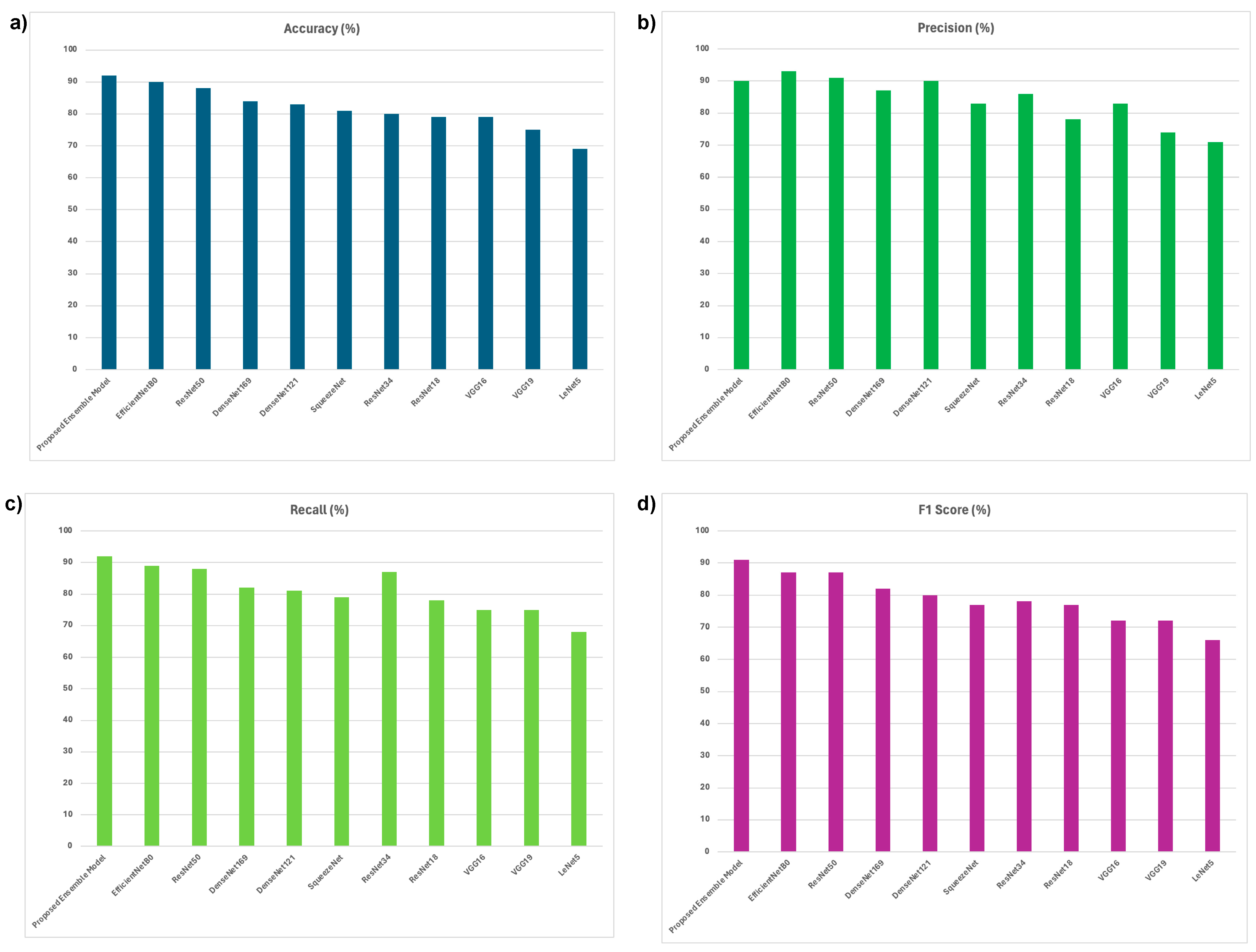
The proposed ensemble model shows better performance with a BS of 64 and a LR of 0.0001 and achieves the highest, i.e., 92% accuracy and 91% F1-score. This indicates that the ensemble method effectively uses the strengths of its constituent models and provides superior performance compared to individual networks. The model also performs well with a BS of 128 and the same LR, achieving an accuracy of 89% and an F1 score of 86%, further highlighting its robustness.

EfficientNetB0 also shows high precision across different configurations, particularly with a BS of 64 and LRs of both 0.001 and 0.0001. It achieves a precision of 97% with a LR of 0.001. ResNet50 performs well with an LR of 0.0001, achieving an accuracy of 88% and an F1 score of 87% with a BS of 64. With a larger batch size of 128, the performance slightly drops. DenseNet169 shows a significant drop in performance with a lower LR of 0.0001, especially with a BS of 64, where the accuracy drops to 65% and the F1 score to 64%. Similarly, DenseNet121 shows poor performance with the same LR. These models highlight the importance of selecting appropriate LRs and BS for optimal performance.

SqueezeNet shows moderate performance, with a decline in accuracy and other metrics at a lower LR of 0.0001. For example, with a BS of 64 and an LR of 0.001, it achieves an accuracy of 81% and an F1 score of 77%, but these metrics drop significantly with a lower LR. The model emphasizes the importance of higher learning rates for maintaining performance. ResNet34 and ResNet18 show stable performance across different settings, though they perform better with an LR of 0.0001 and a BS of 64. ResNet34 achieves an accuracy of 80% and an F1 score of 78% under these conditions. It is observed that these models are versatile and can maintain consistent performance across different configurations.

Both VGG16 and VGG19 show better performance with a higher LR of 0.001. VGG16 achieves an accuracy of 79% and an F1 score of 72% with a BS of 128. The performance of both models drops with a lower LR, indicating these models require higher learning rates to achieve optimal results. LeNet5 shows the lowest performance among the models, particularly with a lower LR. With a BS of 64 and a LR of 0.001, it achieves an accuracy of 69% and an F1 score of 66%. The results indicate that LeNet5 is not recommended for complex datasets. The proposed ensemble model outperforms individual DCNN models, especially at an LR rate of 0.0001 and a batch size of 64 images.

Table 5. Evaluation parameters for each DCNN model and proposed ensemble technique with best batch size and learning rate against each model.

Model	Batch size (BS)	Learning Rate (LR)	Accuracy (%)	Precision (%)	Recall (%)	F1 Score (%)
Proposed Ensemble Model	64	0.0001	92	90	92	91
EfficientNetB0	64	0.0001	90	93	89	87
ResNet50	64	0.0001	88	91	88	87
DenseNet169	64	0.001	84	87	82	82
DenseNet121	64	0.001	83	90	81	80
SqueezeNet	64	0.001	81	83	79	77
ResNet34	64	0.001	80	86	87	78
ResNet18	64	0.001	79	78	78	77
VGG16	128	0.001	79	83	75	72
VGG19	128	0.001	75	74	75	72
LeNet5	64	0.001	69	71	68	66

presents the evaluation parameters for various DCNN models and a proposed ensemble technique using the best batch size and learning rate. The proposed ensemble model demonstrates superior performance with an accuracy of 92% and an F1 score of 91%, using a batch size of 64 and a learning rate of 0.0001. EfficientNetB0 achieves 2% and 4% less accuracy and an F1 score, respectively, under the same hyperparameters. ResNet50 achieves 88% accuracy and recall, whereas an F1 score of 87%. DenseNet169 and DenseNet121 achieve accuracy of 84% and 83%, respectively. SqueezeNet and ResNet34 show moderate performance, with accuracies of 81% and 80%. Overall, the ensemble model outperforms individual models. Figure 4 shows the evaluation parameters as a bar graph to understand the performance of individual models visually.

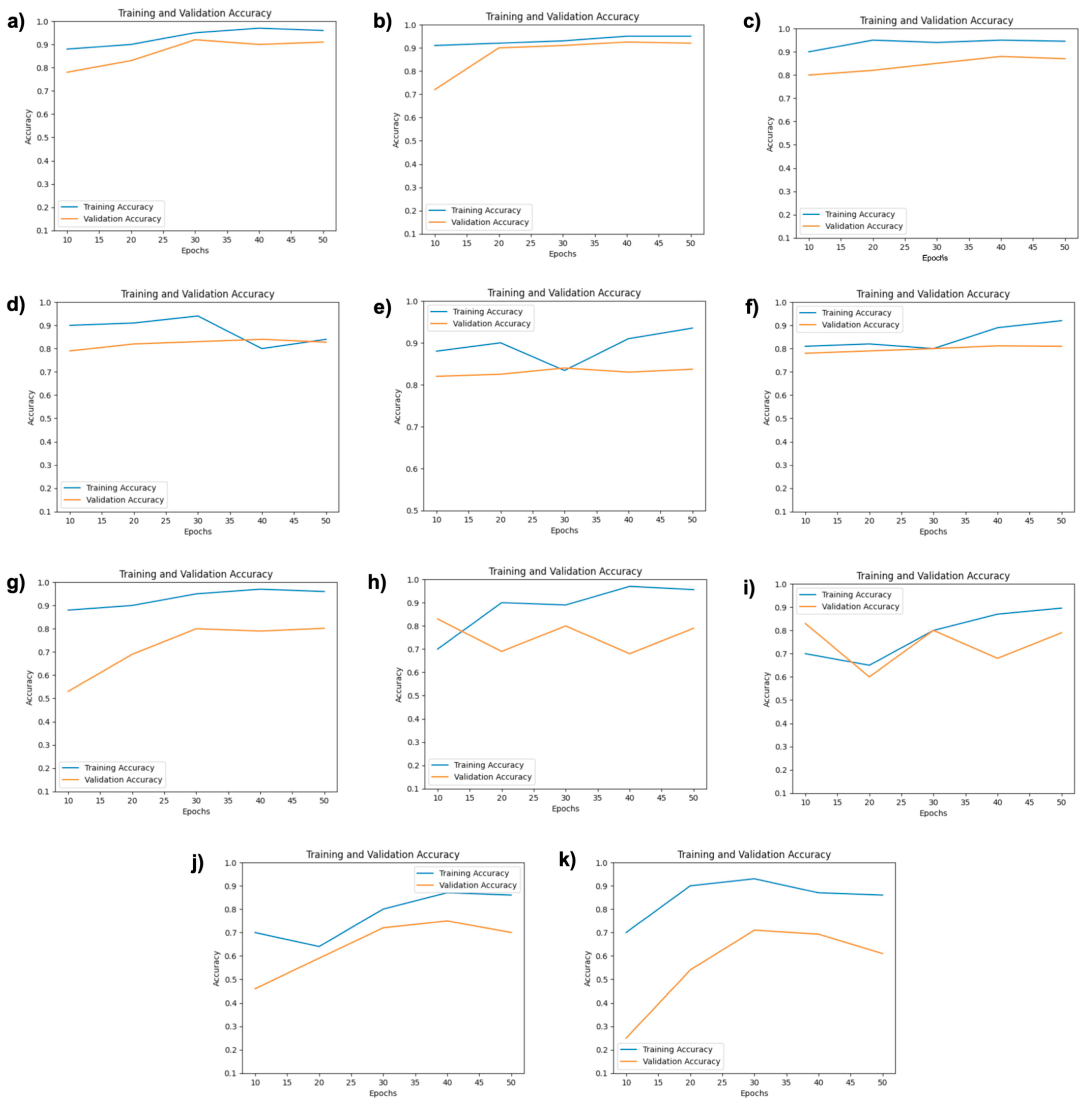
Figure 5 shows the validation accuracy and training accuracy plots for ten DCNN models and our approach using BS and LR. The proposed ensemble model, using a BS of 64 and an LR of 0.0001, shows an increase in accuracy over the epochs, indicating better performance and stability. EfficientNetB0 with a BS of 64 and LR of 0.0001 demonstrates good accuracy but less than the proposed ensemble model. ResNet50 shows a similar trend with robust training and validation accuracy.

DenseNet169, using a BS of 64 and an LR of 0.001, shows a notable performance with increasing accuracy over epochs. Similarly, DenseNet121 under the same conditions illustrates a solid training process but with some fluctuations in validation accuracy. SqueezeNet, also trained with a BS of 64 and an LR of 0.001, indicates a gradual improvement in accuracy, though with some validation instability.

ResNet34, using a BS of 64 and an LR of 0.001, reflects a stable training curve but exhibits some variance in validation accuracy. ResNet18 under similar conditions shows consistent training accuracy but a more varied validation performance. VGG16, with a BS of 128 and a LR of 0.001, shows a relatively steady increase in both training and validation accuracy. VGG19, under the same conditions, shows a comparable pattern with stable improvements. Lastly, LeNet5, using a BS of 64 and an LR of 0.001, indicates moderate performance improvements with some variability in validation accuracy as compared to other models. These plots highlight the robustness of the proposed ensemble method compared to individual DCNN models under various training conditions.

The experimental analysis highlights the importance of appropriate hyperparameter selection, particularly learning rates and batch sizes, in optimizing model performance. The ensemble model’s ability to integrate the strengths of various networks results in a robust and effective solution for high-accuracy tumor and non-tumor MRI classification. The approach has proven its effectiveness for complex MRI datasets.

Comparison of Proposed Ensemble Model vs. Latest Techniques

Table 6. Quantitative comparison of our approach with the latest techniques available in the literature.

Reference	Method	Model	Dataset Medical Modality	Performance
[21], Pareek, M. et al.	Machine Learning	SVM with linear kernal	MRI images	Acc: 78.12
[22], Decuyper, M. et al.	Deep Learning for feature learning and SVM for classification	DL-SVM	MRI images	Acc: 83.30, P: 86.7, R: 79.2
[23], Gupta, M. et al.	Machine Learning	Segmentation-based fractal texture analysis (SFTA)	MRI images	Acc: 87%, P: 88%, R: 86%
[24], Saxena, P. et al.	Deep Learning based DCNN model	(1) VGG16 (2) InceptionV3	MRIs Images	(1) Acc: 90%, P: 90.9% (2) Acc: 55%, P: 68.9%
[25], Cheng, J. et al.	Machine Learning	Spatial Pyramid Matching (SPM)	MRI images	Acc: 91.2%, P:89.7%, R:90.8%, F1: 90%
Proposed Ensemble Technique	Deep Learning	DCNN	MRI images	Acc: 92, P: 90, R: 92, F1: 91

shows a quantitative comparison of our proposed ensemble approach with the latest techniques in the literature for brain tumor classification using MRI images. In [21], Pareek et al. use a machine learning method using an SVM with a linear kernel, achieving 78.12% accuracy. Decuyper et al. [22] combine deep learning for feature learning with SVM for classification, resulting in 83.30% accuracy, 86.7% precision, and 79.2% recall. Gupta et al. [23] utilize a machine learning technique involving segmentation-based fractal texture analysis (SFTA), reporting 87% accuracy, 88% precision, and 86% recall.

Saxena et al. [24] explore deep learning-based DCNN models, specifically VGG16 and InceptionV3, with VGG16 achieving 90% accuracy and 90.9% precision, while InceptionV3 shows lower performance with 55% accuracy and 68.9% precision. Cheng et al. [25] use a machine learning approach using Spatial Pyramid Matching (SPM), having 91.2% accuracy, 89.7% precision, 90.8% recall, and 90% F1-score. Whereas, our proposed ensemble technique uses deep learning, with three DCNN models and achieves superior performance with 92% accuracy, 90% precision, 92% recall, and 91% F1. This comparison highlights the effectiveness of our ensemble approach in enhancing the classification performance of brain tumor detection using MRI images.

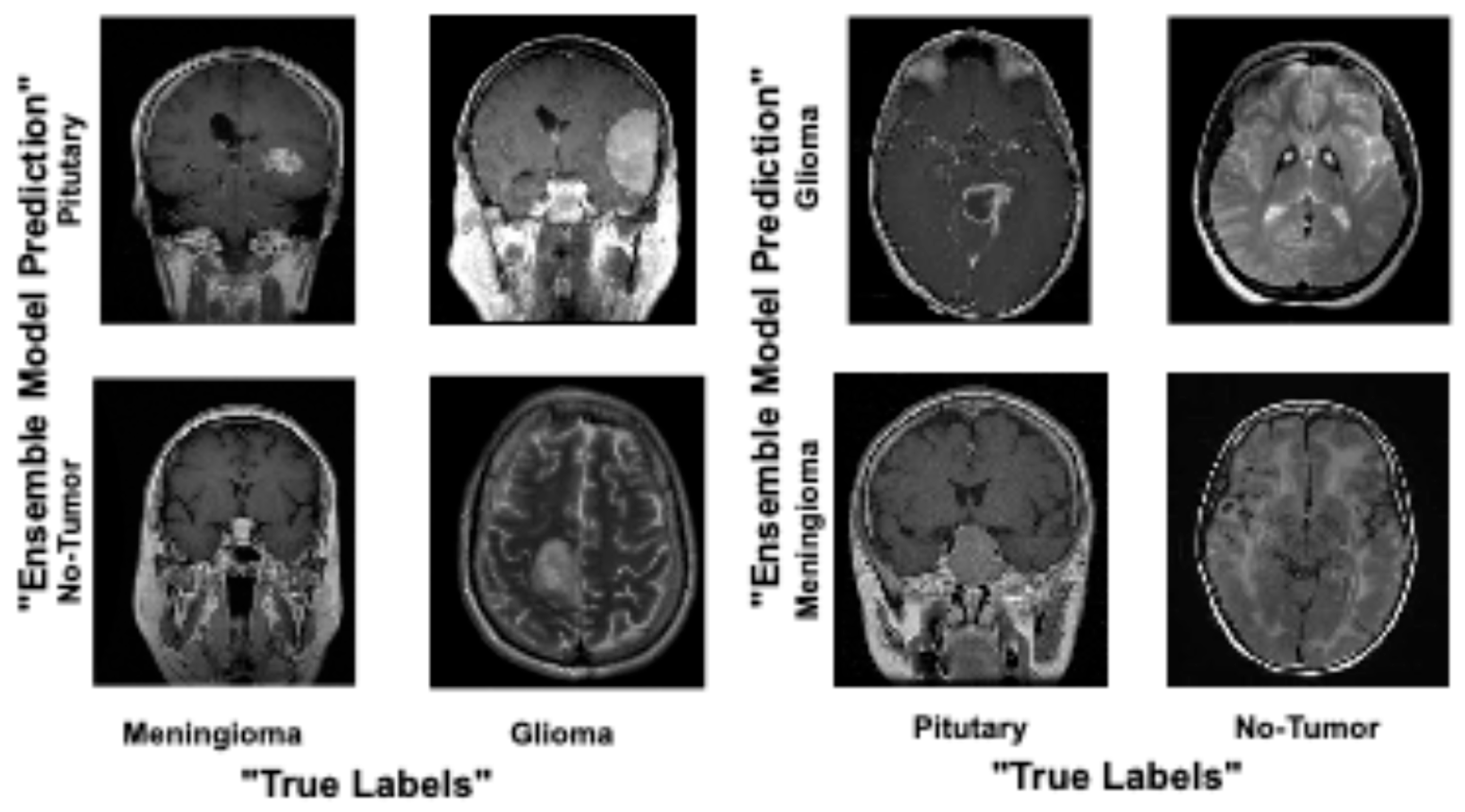
Figure 6 shows the false predictions made by the proposed ensemble technique for MRI classification of brain tumors. There are cases where the model incorrectly identifies the tumor type, such as misclassifying a glioma as a meningioma or failing to detect a non-tumor. Each example in the figure includes the model’s predicted label alongside the actual diagnosis, providing a clear visual comparison of the errors. This allows identifying the specific types of misclassifications the ensemble model is prone to–missing tumors in some cases. It suggests areas where the model may need additional training data or architectural modifications to better distinguish between similar tumor types and avoid false negatives. Analyzing these failure cases is a crucial step in iteratively enhancing the model’s performance for reliable clinical application.

5. Conclusions

An ensemble of three well-performing DCNN models, i.e., DenseNet169, EfficientNetB0, and ResNet50, is shown in this study for the accurate classification of tumors (glioma, meningioma, and pituitary) and non-tumor MRI samples. Our proposed ensemble model significantly improves classification accuracy, precision, recall, and F1 score compared to individual SOTA DCNN models. We implemented and compared ten SOTA models and evaluated them with two LR and two BS to identify optimal hyperparameters for each model. The ensemble model outperformed compared to other well-known DCNN models at a BS of 64 and an LR of 0.0001. We also highlighted the better performance of our approach and provided a comparison with the latest research. We used only a single dataset, which may reduce the generalizability of our findings. While our ensemble approach may perform well on this particular dataset, their performance across different datasets, especially those with varying characteristics, such as image quality, noise levels, or class imbalance, remains untested. Expanding this study to multiple datasets and a wider range of hyperparameters could provide more robust and comprehensive insights into the optimal settings for the SOTA DCNN models and our ensemble approach.

As a future direction, considering the limitations of our study, we aim to expand this study by including diverse datasets with varying characteristics, such as different image qualities, noise levels, and class imbalances. They are crucial to improving the generalizability of our findings. Additionally, exploring a wider range of hyperparameters beyond the two learning rates and batch sizes we used could help identify optimal configurations for DCNN models and further refine our ensemble approach [26]. This would provide more comprehensive insights into model performance across a variety of real-world scenarios.

References

1. Mukadam, S.B.; Patil, H.Y. Machine learning and computer vision based methods for cancer classification: A systematic review. Arch. Comput. Methods Eng. 2024, 31, 3015–3050. [Google Scholar] [CrossRef]
2. International Agency for Research on Cancer. Cancer Today. 2023. Available online: https://gco.iarc.fr/today/data/factsheets/cancers/20-Brain.cancer (accessed on 16 April 2024).
3. Raza, A.; Khan, M.U.; Saeed, Z.; Samer, S.; Mobeen, A.; Samer, A. Classification of eye diseases and detection of cataract using digital fundus imaging (DFI) and inception-V4 deep learning model. In Proceedings of the 2021 International Conference on Frontiers of Information Technology (FIT), Islamabad, Pakistan, 13–14 December 2021; IEEE: New York, NY, USA, 2021; pp. 137–142. [Google Scholar]
4. Saeed, Z.; Khan, M.U.; Raza, A.; Khan, H.; Javed, J.; Arshad, A. Classification of pulmonary viruses X-ray and detection of COVID-19 based on invariant of inception-V 3 deep learning model. In Proceedings of the 2021 International Conference on Computing, Electronic and Electrical Engineering (ICE Cube), Quetta, Pakistan, 26–27 October 2021; IEEE: New York, NY, USA, 2021; pp. 1–6. [Google Scholar]
5. Naqvi, S.Z.H.; Khan, M.U.; Raza, A.; Saeed, Z.; Abbasi, Z.; Ali, S.Z.E.Z. Deep Learning Based Intelligent Classification of COVID-19 & Pneumonia Using Cough Auscultations. In Proceedings of the 2021 6th International Multi-Topic ICT Conference (IMTIC), Jamshoro & Karachi, Pakistan, 10–12 November 2021; IEEE: New York, NY, USA, 2021; pp. 1–6. [Google Scholar]
6. Byun, Y.H.; Ha, J.; Kang, H.; Park, C.K.; Jung, K.W.; Yoo, H. Changes in the Epidemiologic Pattern of Primary CNS Tumors in Response to the Aging Population: An Updated Nationwide Cancer Registry Data in the Republic of Korea. JCO Glob. Oncol. 2024, 10, e2300352. [Google Scholar] [CrossRef] [PubMed]
7. Srinivas, C.; KS, N.P.; Zakariah, M.; Alothaibi, Y.A.; Shaukat, K.; Partibane, B.; Awal, H. Deep transfer learning approaches in performance analysis of brain tumor classification using MRI images. J. Healthc. Eng. 2022, 2022, 3264367. [Google Scholar] [CrossRef] [PubMed]
8. Khairandish, M.O.; Sharma, M.; Jain, V.; Chatterjee, J.M.; Jhanjhi, N.Z. A hybrid CNN-SVM threshold segmentation approach for tumor detection and classification of MRI brain images. Irbm 2022, 43, 290–299. [Google Scholar] [CrossRef]
9. Khan, A.H.; Abbas, S.; Khan, M.A.; Farooq, U.; Khan, W.A.; Siddiqui, S.Y.; Ahmad, A. Intelligent model for brain tumor identification using deep learning. Appl. Comput. Intell. Soft Comput. 2022, 2022, 8104054. [Google Scholar] [CrossRef]
10. Assam, M.; Kanwal, H.; Farooq, U.; Shah, S.K.; Mehmood, A.; Choi, G.S. An efficient classification of MRI brain images. IEEE Access 2021, 9, 33313–33322. [Google Scholar] [CrossRef]
11. Noreen, N.; Palaniappan, S.; Qayyum, A.; Ahmad, I.; Imran, M.; Shoaib, M. A deep learning model based on concatenation approach for the diagnosis of brain tumor. IEEE Access 2020, 8, 55135–55144. [Google Scholar] [CrossRef]
12. Ghassemi, N.; Shoeibi, A.; Rouhani, M. Deep neural network with generative adversarial networks pre-training for brain tumor classification based on MR images. Biomed. Signal Process. Control 2020, 57, 101678. [Google Scholar] [CrossRef]
13. Musallam, A.S.; Sherif, A.S.; Hussein, M.K. A new convolutional neural network architecture for automatic detection of brain tumors in magnetic resonance imaging images. IEEE Access 2022, 10, 2775–2782. [Google Scholar] [CrossRef]
14. Ismael SA, A.; Mohammed, A.; Hefny, H. An enhanced deep learning approach for brain cancer MRI images classification using residual networks. Artif. Intell. Med. 2020, 102, 101779. [Google Scholar] [CrossRef] [PubMed]
15. Sekhar, A.; Biswas, S.; Hazra, R.; Sunaniya, A.K.; Mukherjee, A.; Yang, L. Brain tumor classification using fine-tuned GoogLeNet features and machine learning algorithms: IoMT enabled CAD system. IEEE J. Biomed. Health Inform. 2021, 26, 983–991. [Google Scholar] [CrossRef] [PubMed]
16. Irmak, E. Multi-classification of brain tumor MRI images using deep convolutional neural network with fully optimized framework. Iran. J. Sci. Technol. Trans. Electr. Eng. 2021, 45, 1015–1036. [Google Scholar] [CrossRef]
17. Kaggle Dataset. Available online: https://www.kaggle.com/datasets/masoudnickparvar/brain-tumor-mri-dataset (accessed on 13 August 2023).
18. Mahesh, T.R.; Vinoth Kumar, V.; Vivek, V.; Karthick Raghunath, K.M.; Sindhu Madhuri, G. Early predictive model for breast cancer classification using blended ensemble learning. Int. J. Syst. Assur. Eng. Manag. 2024, 15, 188–197. [Google Scholar] [CrossRef]
19. Bai, Y.; Zhang, X.; Wang, Q.; Lv, J.; Chen, L.; Du, Y.; Du, L. An Area-Efficient CNN Accelerator Supporting Global Average Pooling with Arbitrary Shapes. In Proceedings of the 2024 IEEE 6th International Conference on AI Circuits and Systems (AICAS), Abu Dhabi, The United Arab Emirates, 22–25 April 2024; IEEE: New York, NY, USA, 2024. [Google Scholar]
20. Hussain, D.; Al-Masni, M.A.; Aslam, M.; Sadeghi-Niaraki, A.; Hussain, J.; Gu, Y.H.; Naqvi, R.A. Revolutionizing tumor detection and classification in multimodality imaging based on deep learning approaches: Methods, applications and limitations. J. X-ray Sci. Technol. 2024, 32, 857–911. [Google Scholar] [CrossRef] [PubMed]
21. Pareek, M.; Jha, C.K.; Mukherjee, S. Brain tumor classification from MRI images and calculation of tumor area. In Soft Computing: Theories and Applications: Proceedings of SoCTA 2018; Springer: Singapore, 2020; pp. 73–83. [Google Scholar]
22. Decuyper, M.; Bonte, S.; Deblaere, K.; Van Holen, R. Automated MRI based pipeline for glioma segmentation and prediction of grade, IDH mutation and 1p19q co-deletion. arXiv 2020, arXiv:2005.11965. [Google Scholar] [CrossRef] [PubMed]
23. Gupta, M.; Sasidhar, K. Non-invasive brain tumor detection using magnetic resonance imaging based fractal texture features and shape measures. In Proceedings of the 2020 3rd International Conference on Emerging, Kolkata, India, 23–25 February 2020. [Google Scholar]
24. Saxena, P.; Maheshwari, A.; Maheshwari, S. Predictive modeling of brain tumor: A deep learning approach. In Innovations in Computational Intelligence and Computer Vision: Proceedings of ICICV 2020; Springer: Singapore, 2020; pp. 275–285. [Google Scholar]
25. Cheng, J.; Huang, W.; Cao, S.; Yang, R.; Yang, W.; Yun, Z.; Wang, Z.; Feng, Q. Enhanced performance of brain tumor classification via tumor region augmentation and partition. PLoS ONE 2015, 10, e0140381. [Google Scholar] [CrossRef] [PubMed]
26. Saeed, Z.; Bouhali, O.; Ji, J.X.; Hammoud, R.; Al-Hammadi, N.; Aouadi, S.; Torfeh, T. Cancerous and Non-Cancerous MRI Classification Using Dual DCNN Approach. Bioengineering 2024, 11, 410. [Google Scholar] [CrossRef] [PubMed]
Figure 1. Block diagram of our proposed methodology.
Information 15 00641 g001
Figure 2. Dataset samples (a) No tumor, (b) Glioma, (c) Meningioma, and (d) Pituitary.
Information 15 00641 g002
Figure 3. Overall dataset distribution against each class.
Information 15 00641 g003
Figure 4. (a) Accuracy, (b) Precision, (c) Recall, (d) F1-Score of Proposed Ensemble Model using 64 BS and 0.0001 LS, EfficientNetB0 using 64 BS and 0.0001, ResNet59 using 64 BS and 0.0001, DenseNet169, DenseNet121 using 64 BS and 0.001, SqueezeNet using 64 BS and 0.001, ResNet34 using 64 BS and 0.001, ResNet18 using 64 BS and 0.001, VGG16 using 128 BS and 0.001, VGG18 using 128 BS and 0.001, LeNet5 using 64 BS and 0.001.
Information 15 00641 g004
Figure 5. Training and Validation plots of (a) Proposed Ensemble Model using 64 BS and 0.0001 LS, (b) EfficientNetB0 using 64 BS and 0.0001, (c) ResNet59 using 64 BS and 0.0001, (d) DenseNet169 using 64 BS and 0.001, (e) DenseNet121 using 64 BS and 0.001, (f) SqueezeNet using 64 BS and 0.001, (g) ResNet34 using 64 BS and 0.001, (h) ResNet18 using 64 BS and 0.001, (i) VGG16 using 128 BS and 0.001, (j) VGG18 using 128 BS and 0.001, (k) LeNet5 using 64 BS and 0.001.
Information 15 00641 g005
Figure 6. False predictions of Proposed Ensemble Technique.
Information 15 00641 g006