Abstract
Support vector regression (SVR) is a powerful kernel-based regression prediction algorithm that performs excellently in various application scenarios. However, for real-world data, the general SVR often fails to achieve good predictive performance due to its inability to assess feature contribution accurately. Feature weighting is a suitable solution to address this issue, applying correlation measurement methods to obtain reasonable weights for features based on their contributions to the output. In this paper, based on the idea of a Hilbert–Schmidt independence criterion least absolute shrinkage and selection operator (HSIC LASSO) for selecting features with minimal redundancy and maximum relevance, we propose a novel feature-weighted SVR that considers the importance of features to the output and the redundancy between features. In this approach, the HSIC is utilized to effectively measure the correlation between features as well as that between features and the output. The feature weights are obtained by solving a LASSO regression problem. Compared to other feature weighting methods, our method takes much more comprehensive consideration of weight calculation, and the obtained weighted kernel function can lead to more precise predictions for unknown data. Comprehensive experiments on real datasets from the University of California Irvine (UCI) machine learning repository demonstrate the effectiveness of the proposed method.
1. Introduction
Support vector regression (SVR) is a powerful kernel-based technique for solving the problem of regression estimation [1,2]. SVR was initially proposed by Vapnik and his collaboration partners based on the concept of support vectors [3,4]. It promotes the support vector machine (SVM) grounded in statistical learning and Vapnik-Chervonenkis (VC) theory and returns a continuous-valued output instead of an output from a finite set [5]. As a supervised learning method, SVR avoids the overfitting problem by adopting the principle of structural risk minimization, and the computational complexity of SVR does not depend on the dimensionality of the input space [6,7]. Due to its outstanding performance in many aspects, SVR has currently become a widely used tool in regression prediction analysis, in which it is used for analyzing financial data trends [8,9], forecasting time series [10,11], and predicting engineering energy consumption [12,13]. In general, its good generalization ability makes it popular in the machine learning and data mining community [14].
Assigning certain weights to each feature in a dataset based on a specific criterion is called feature weighting [15]. It assumes that the contributions of different dimensional features of the sample vector to the regression task are different [16]. During SVR training, each feature is assigned a weight corresponding to its contribution to the output, resulting in a more robust model known as feature-weighted SVR (FWSVR). Since the generalization ability of SVR is determined by the features in kernel space, ensuring features are weighted is an effective way to build a more potent model [17,18]. Compared with SVR, FWSVR considers the importance of feature variables relative to predicted labels. Additionally, to a certain extent, weights reflect the impact of features on the regression results. Therefore, reasonable measures for quantifying the correlation between features and output are crucial in feature weighting algorithms.
In recent years, there has been active research on FWSVR and its applications. Liu and Hu [19] introduced an FWSVR based on the gray correlation degree (GCD) for stock price prediction. The key idea of the GCD method is to assess the correlation between two variables by evaluating the similarity of the geometric shapes of their sequence curves. Hou et al. [20] proposed a modified SVR with a maximal information coefficient (MIC)-weighted kernel. MIC is employed to measure the correlation of both linear and nonlinear relationships between input and output [21]. Xie et al. [22] proposed a FWSVR based on MIC and particle swarm optimization (PSO) algorithm [23]. In this method, the MIC of each feature is calculated to reveal its contribution to the output, and both weights and parameters are tuned by a constrained PSO. Pathak et al. [24,25] used an efficient learning method called reservoir computing (RC) to make model-free predictions of chaotic systems based solely on the knowledge of past states. This method can predict the future state of the system by analyzing data correlation without explicit prior knowledge, which is very instructive for the calculation of feature weights.
There are also many methods for calculating weights in feature-weighted SVM (FWSVM) [16,26,27]. However, these methods cannot be directly applied to regression tasks because they are primarily designed to enhance algorithmic learning for classification. Moreover, in regression problems, the output consists of a series of continuous values, whereas in classification problems, the output typically comprises integer values representing class labels. The aim of our study is to design a new FWSVR algorithm for regression problems.
For the feature weighting algorithm, the method of evaluating feature weights is crucial, as it directly determines the predictive performance of the model. However, the feature weighting methods mentioned above only use the correlation between features and outputs as the basis for evaluating feature weights, ignoring the redundancy between different features. Inspired by the HSIC LASSO, which finds the features with the greatest dependence on the output value and the least redundancy through HSIC [28,29,30,31], we present a HSIC LASSO-based feature weighting method for SVR called HL-FWSVR. In this method, the correlations between features and those between features and the output are measured by HSIC. Our method simultaneously incorporates the redundancy among the features and the correlation between features and output into the evaluation of feature weights. Besides, HSIC LASSO has a clear statistical interpretation and is a convex optimization problem, in which the global optimal solution can be efficiently calculated by solving a LASSO optimization problem.
The remainder of the paper is organized as follows. In the next section, we briefly review SVR and focus on the HSIC LASSO optimization problem. The process of calculating the feature-weighted kernel function and constructing FWSVR is presented in Section 3. In Section 4, we conduct experiments comparing the proposed algorithm with the previously excellent FWSVR algorithms on public datasets. The general conclusion and directions for future work are discussed in Section 5.
2. Preliminaries
In this section, we briefly review some preliminaries on SVR and HSIC LASSO.
2.1. Review of SVR
Given a training set , ( represents the number of samples, denotes the set of real numbers and is the number of original features) represents the input data and is the target output. SVR seeks to learn a regression model in the kernel space in the form of Equation (1), where maps the input features to a high-dimensional kernel space, is the normal vector, and is the bias term.
In SVR, an insensitive loss is introduced to avoid overfitting, and nonnegative slack variables and are adopted to weaken the constraints of some certain sample points. Specifically, SVR can be formulated as a convex quadratic programming problem expressed as follows:
where is a penalty parameter, and ‘s.t’ stands for ‘subject to’ followed by the constraints. The above constrained quadratic programming problem can be solved by its dual problem, as shown in Equation (3):
where are Lagrange multipliers and is the kernel function (kernel matrix is defined as ). Several commonly used kernel functions are listed in Table 1.

Table 1.
Commonly used kernel functions.
Finally, the decision function can be expressed as follows:
2.2. HSIC LASSO
HSIC LASSO was first introduced by Yamada et al. [30] for feature selection. Given a weight vector , suppose represents the input data which have samples with features and is the output label vector, and are corresponding kernel matrices that are respectively defined on the input data and output vector . HSIC LASSO is given by
where is the Frobenius norm, is a regression coefficient vector and denotes the regression coefficient of the -th feature, is the regularization parameter, and are centered Gram matrices ( is the centering matrix, where and are the vector of ones and the identity matrix, respectively), and is the kernel matrix on the feature for all samples. In Equation (5), the first term indicates that the linear combination of the centered kernel matrices (one feature associates with a kernel) for the input data is aligned with the centered kernel matrix for the output label, and the second term indicates that the weights (combination coefficients) for the irrelevant features (kernels) tend to be zero, since the norm is inclined to generate a sparse solution.
HSIC LASSO can be regarded as a minimum redundancy maximum relevancy (mRMR)-based method [32]. The first term in Equation (5) can be rewritten as
where is the vector of the feature for all samples, is a kernel-based independence measure called the empirical HSIC [29], and denotes the trace. HSIC always takes a nonnegative value, and is zero if and only if two random variables are statistically independent. The empirical HSIC asymptotically converges to the true HSIC with [29].
In Equation (6), is a constant and can be ignored. If the -th feature exhibits a high dependency on the output , takes a large value; thus, should also take a large value so that Equation (5) is minimized. On the other hand, if is independent of , takes a small value and, thus, tends to be zero as a result of the -regularizer. Moreover, if and are highly correlated (i.e., redundant features), takes a large value and thus either or tends to be zero. This implies that HSIC LASSO considers both the importance of features on the output and the correlation among features.
3. Training FWSVR with HSIC LASSO
3.1. Modifying Kernel Function
The generalization performance of SVR largely depends on a key component, namely the kernel function, which maps the input data into a high-dimensional feature space. This mapping is implicitly defined by the kernel function, thus selecting the appropriate kernel function is crucial when training an SVR [33]. There are simple examples illustrating that constructing such a kernel space by only considering the feature values of samples and ignoring their contributions to the model output is unreasonable [18]. Therefore, we apply feature weighting to match the impact of features in kernel space with their contributions to the model output. For the -th feature, if its feature weight is calculated using a weighting metric method, the form of the feature-weighted kernel function is as follows:
where the linear transformation matrix serves as the feature weighting matrix, and choosing different shapes of will lead to different weighting scenarios [16]. In this paper, we only consider the diagonal matrix situation, shown in Equation (8), where .
Based on Equation (7), the commonly used kernel functions can be rewritten as the feature-weighted kernel functions. For example, if a Gaussian kernel is selected, the weighted form is given as follows:
3.2. Constructing HL-FWSVR
The relative positions between sample points will correspondingly change given a set of weight values for features. More specifically, changes in the positional relationships alter the shape of the Euclidean feature space, thereby creating conditions conducive to improving the performance of SVR. The steps for constructing FWSVR based on HSIC LASSO are summarized in Table 2.

Table 2.
Algorithm of the proposed HL-FWSVR.
In Step 3, as a universal kernel (such as a Gaussian kernel or Laplacian kernel) enables HSIC to detect the dependency between two random variables [29]. In this paper, the Gaussian kernel is selected for the input . For the output , the Gaussian kernel is commonly applied in regression scenarios, while the Delta kernel is used for classification problems. In this paper, the Gaussian kernel is also selected for the output . In summary, since we consider the regression scenario, the kernels described in Equations (10) and (11) are utilized, where and are the Gaussian kernel widths.
In Step 4, based on the computational properties of HSIC LASSO, the dual augmented Lagrangian (DAL) [34] can efficiently solve the HSIC LASSO problem when the number of features is relatively large. Conversely, when the number of samples is relatively large, we employ the feature vector machine (FVM) [35] formulation. In our work, we use Python implementation of an HSIC LASSO named pyHSICLasso to tackle the problem (details on the usage of pyHSICLasso can be found at https://pypi.org/project/pyHSICLasso).
4. Experiments
In this section, we perform extensive experiments on several real-world regression datasets to evaluate the efficacy of the proposed HL-FWSVR approach. All the codes are compiled on a laptop with 8 GB memory and Inter (R) Core (TM) i5-7300HQ 2.50 Ghz CPU by using PyCharm (Community Edition 2023.1.1).
4.1. Comparison Approaches and Evaluation Criteria
We compare HL-FWSVR with the following learning methods:
- SVR: The classical SVR machine.
- GCD-FWSVR: A feature-weighted SVR machine with correlation between input and output evaluated by GCD [19].
- MIC-FWSVR: The MIC is applied to obtain the weighted kernel of SVR, which can measure the linear and nonlinear correlation between two variables [20].
- MP-FWSVR: The feature weighting method of this approach adopts a PSO algorithm [22]. The MIC of each feature is calculated to constrain the search range of weights. It is an improved PSO search method.
The root mean squared error (RMSE) is considered to be an essential statistical metric to evaluate the prediction performance of the regression algorithm. It measures the deviation between the actual values and the predicted ones. A smaller RMSE value indicates a better fitting effect of the model [36]. The coefficient of determination (R2 or R-Squared) is selected as the other performance metric. R2 can be interpreted as the proportion of the variance in the dependent variable that is predictable from the independent variables, and its worst value is and best value is 1 [36]. A value closer to 1 indicates a better model fit. The RMSE and R2 are formally defined as follows:
4.2. Experiment Setup
We select eight popular datasets, i.e., Servo (which contains data on the servo motor’s angle based on certain inputs), Auto MPG (which relates to different car models and their fuel efficiency), Qualitative Structure–Activity Relationships (which addresses the activity of chemical compounds based on their molecular structures), Bodyfat (which comprises measurements related to body fat percentage), Boston Housing (which contains information about housing values in suburbs of Boston), Facebook Metrics (the Facebook performance metrics of a renowned cosmetic’s brand Facebook page), Energy Efficiency (assessments on the heating load and cooling load requirements of buildings), and Concrete Compressive Strength (the composition of concrete and its compressive strength), from the University of California Irvine (UCI) machine learning repository [37]. For each dataset, we exclude samples with missing values from the original dataset. Table 3 presents the statistical information for these datasets. The abbreviations for each dataset, along with the sample size (numbers of samples for the training set (S) and test set (T) in parentheses), the number of features, and the original names of the datasets, are provided.

Table 3.
Statistics of the selected eight datasets.
Before the model is trained, Min–Max scaling is applied to normalize the features to the range of [−1, 1]. All the algorithms utilize the Gaussian kernel for model construction. The regularization parameter , kernel parameter , and margin of tolerance play pivotal roles in shaping the performance of SVR. Inspired by the MP-FWSVR, we employ the PSO algorithm (instead of the commonly used grid search) to search for the model parameters on the training set S, and use ten-fold cross validation (9/10 of S is used as the training set and 1/10 of S is used as the test set in each fold) as the fitness function of PSO to determine whether the current position is optimal [23]. Subsequently, we use the obtained optimal parameters to construct an FWSVR model on S. The performance of the model will finally be tested on the test set T.
4.3. Results and Discussion
The RMSE and R2 results for each algorithm are presented in Table 4, and the bold numbers highlight the best performance of these methods on each dataset. The average performance ranking of each algorithm is also attached at the bottom of Table 4. It is evident that FWSVR generally outperforms the classical SVR in regression tasks. This suggests that assigning appropriate weights to features based on their contributions to the output can indeed enhance the predictive performance of regression algorithms. Another important consideration is that, compared to other baseline approaches, our proposed HL-FWSVR consistently demonstrates the best overall prediction performance. Of the eight datasets evaluated, GCD-FWSVR reports two best results and MP-FWSVR reports one best result, while our HL-FWSVR reports five best results. Moreover, as for the R2 results, the proposed HL-FWSVR can explain more than 96% and 99% of the variation in the results of the predictor variables on the Bodyfat dataset and Energy dataset, respectively. In particular, for the Facebook dataset, the result surpasses 98%, while the suboptimal model MP-FWSVR only reaches approximately 66%, indicating that our model has a significantly better fitting effect on this dataset compared to other models.

Table 4.
RMSE and R2 comparison of different algorithms.
In order to provide a clearer observation of the performance differences among different algorithms, we plot the prediction curves and distributions of feature weights of different models on these eight datasets, which are shown in Figure 1, Figure 2, Figure 3, Figure 4, Figure 5, Figure 6, Figure 7, Figure 8, Figure 9, Figure 10, Figure 11, Figure 12, Figure 13, Figure 14, Figure 15 and Figure 16 (F1 represents the first feature, F2 represents the second feature, and so on). In the prediction curve charts, the horizontal axis is the serial number of the sample point and the vertical axis is the model output. It is apparent from the sub-figures (d) that our model has a better fitting performance on some datasets; for example, Servo, Pyrim, and Facebook. As for the distribution of feature weights, it can be seen that the weights obtained by the HL-FWSVR are more dispersed, the standard deviation of the weight values is larger, and the differences are more pronounced. To some extent, the higher fluctuation in the weight values indicates that the HL-FWSVR model more effectively considers the correlation between features and the redundancy among features, thereby avoiding the influence of irrelevant and redundant features in calculating feature-weighted kernel functions. It should also be noted that, for the HL-FWSVR method, due to the influence of the LASSO regularization term, some of feature weights are shrunk to 0.
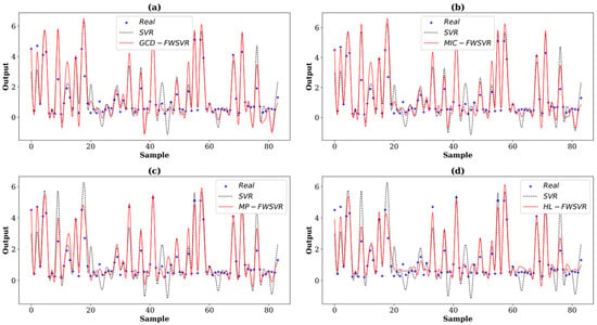
Figure 1.
Prediction curves of different algorithms on the Servo dataset. The (a–d) show the prediction comparison between SVR and GCD-FWSVR, MIC-FWSVR, MP-FWSVR, and HL-FWSVR, respectively.
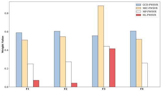
Figure 2.
Feature weights of different models on the Servo dataset.
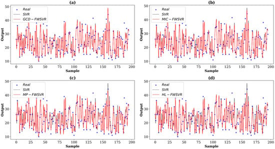
Figure 3.
Prediction curves of different algorithms on the Mpg dataset. The (a–d) show the prediction comparison between SVR and GCD-FWSVR, MIC-FWSVR, MP-FWSVR, and HL-FWSVR, respectively.
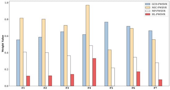
Figure 4.
Feature weights of different models on the Mpg dataset.
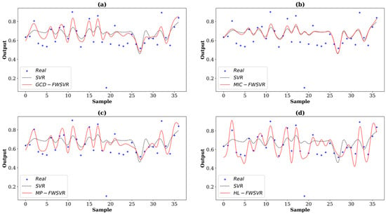
Figure 5.
Prediction curves of different algorithms on the Pyrim dataset. The (a–d) show the prediction comparison between SVR and GCD-FWSVR, MIC-FWSVR, MP-FWSVR, and HL-FWSVR, respectively.
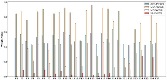
Figure 6.
Feature weights of different models on the Pyrim datasets.
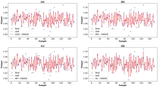
Figure 7.
Prediction curves of different algorithms on the Bodyfat dataset. The (a–d) show the prediction comparison between SVR and GCD-FWSVR, MIC-FWSVR, MP-FWSVR, and HL-FWSVR, respectively.
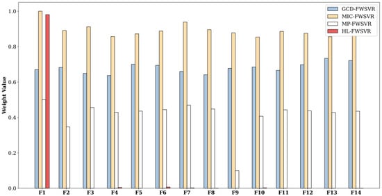
Figure 8.
Feature weights of different models on the Bodyfat dataset.
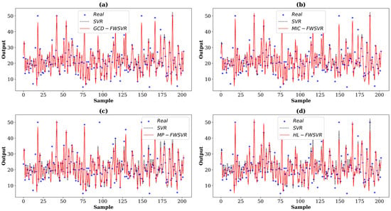
Figure 9.
Prediction curves of different algorithms on the Boston dataset. The (a–d) show the prediction comparison between SVR and GCD-FWSVR, MIC-FWSVR, MP-FWSVR, and HL-FWSVR, respectively.
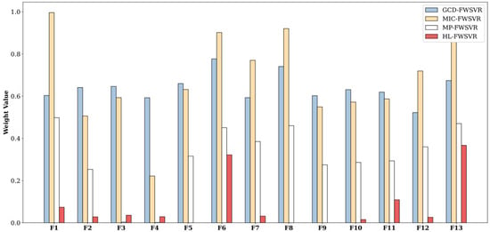
Figure 10.
Feature weights of different models on the Boston dataset.
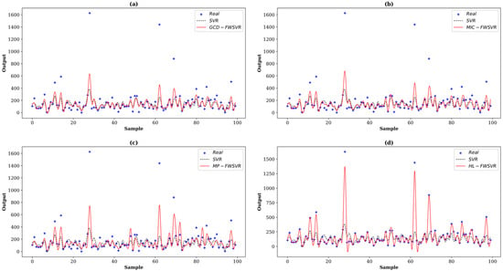
Figure 11.
Prediction curves of different algorithms on the Facebook dataset. The (a–d) show the prediction comparison between SVR and GCD-FWSVR, MIC-FWSVR, MP-FWSVR, and HL-FWSVR, respectively.
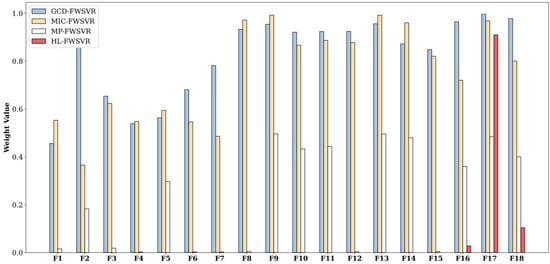
Figure 12.
Feature weights of different models on the Facebook dataset.
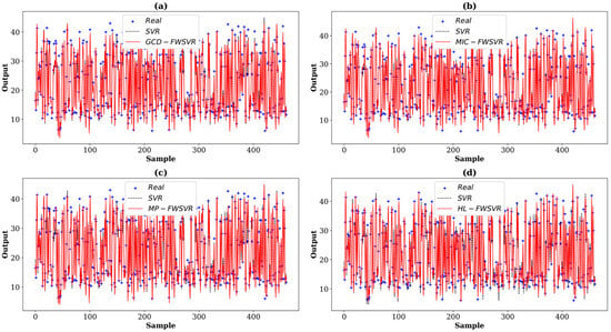
Figure 13.
Prediction curves of different algorithms on the Energy dataset. The (a–d) show the prediction comparison between SVR and GCD-FWSVR, MIC-FWSVR, MP-FWSVR, and HL-FWSVR, respectively.
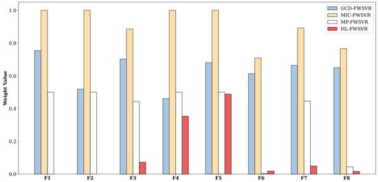
Figure 14.
Feature weights of different models on the Energy dataset.
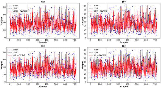
Figure 15.
Prediction curves of different algorithms on the Concrete dataset. The (a–d) show the prediction comparison between SVR and GCD-FWSVR, MIC-FWSVR, MP-FWSVR, and HL-FWSVR, respectively.
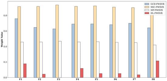
Figure 16.
Feature weights of different models on the Concrete dataset.
To summarize, our proposed HL-FWSVR achieves the best overall prediction results on these benchmark datasets. We attribute the superior performance to the fact that HSIC LASSO has the advantage of identifying features that are relevant to the output, but remain independent of each other. Unlike our method, the baseline approaches only consider the correlation between features and output, while the redundancy between different features is neglected. Besides, the MP-FWSVR mothed employs heuristic search strategies which tend to produce local optima, while our method can determine the globally optimal solution.
5. Conclusions and Future Work
This paper proposes an effective HSIC LASSO-based FWSVR model called HL-FWSVR. In the proposed model, HSIC LASSO is introduced as a method for measuring feature weights, thereby computing the weighted kernel function to obtain the FWSVR model for predicting regression data. The essential advantage of the proposed HL-FWSVR model lies in the fact that the calculated feature weights not only reflect the contributions of features to the output but also consider the redundancy among features. We conduct comprehensive experiments on several regression datasets, and the proposed method yields promising results.
With regard to future work, price time series forecasting is currently an important and complex area of machine learning [38]. The fact that price evolution has a time component adds additional information to the forecast, which means that the model needs to be able to handle new complexities that are not present in other forecasting tasks. Therefore, our next step will be to extend the application of HSIC LASSO to time series forecasting, such as weather forecasting and stock indices. Also, we will further investigate the proposed HL-FWSVR in high-dimensional scenarios like text datasets and biological gene datasets. While dimensionality reduction is not a good choice in scenarios with unclear domain knowledge, it is necessary to utilize feature weighting to fully consider the importance of features and avoid losing any potentially important information. Furthermore, feature weights also affect the selection of kernel parameters. Methods of obtaining the optimal kernel parameters that match the optimal weight values are also worthy of exploration.
Author Contributions
Conceptualization, X.Z. and T.W.; Methodology, X.Z. and T.W.; Software, X.Z. and Z.L.; Validation, X.Z. and T.W.; Formal analysis, X.Z. and T.W.; Investigation, X.Z. and T.W.; Resources, X.Z., T.W. and Z.L.; Data curation, X.Z. and Z.L.; Writing—original draft, X.Z.; Writing—review and editing, X.Z. and T.W.; Visualization, X.Z.; Supervision, T.W.; Project administration, T.W. All authors have read and agreed to the published version of the manuscript.
Funding
This work is supported in part by the Natural Science Foundation of Jiangxi Province of China (No. 20242BAB26024), the Graduate Innovation Special Foundation of Jiangxi Province of China (No. YC2023-S865), and the Program of Academic Degree and Graduate Education and Teaching Reform in Jiangxi Province of China (No. JXYJG-2022-172).
Institutional Review Board Statement
Not applicable.
Informed Consent Statement
Not applicable.
Data Availability Statement
The datasets used in this study can be accessed from the UCI machine learning repository, as referenced in [37].
Conflicts of Interest
The authors declare no conflicts of interest.
References
- Vapnik, V. An overview of statistical learning theory. IEEE Trans. Neural Netw. 1999, 10, 988–999. [Google Scholar] [CrossRef] [PubMed]
- Drucker, H.; Burges, C.J.; Kaufman, L.; Smola, A.; Vapnik, V. Support vector regression machines. Adv. Neural Inf. Process. Syst. 1996, 9, 155–161. [Google Scholar]
- Vapnik, V. The Nature of Statistical Learning Theory; Springer Science and Business Media: Berlin/Heidelberg, Germany, 2013. [Google Scholar]
- Cortes, C.; Vapnik, V. Support-vector networks. Mach. Learn. 1995, 20, 273–297. [Google Scholar] [CrossRef]
- Awad, M.; Khanna, R. Support vector regression. In Efficient Learning Machines; Apress: Berkeley, CA, USA, 2015. [Google Scholar]
- Vapnik, V. Principles of risk minimization for learning theory. Adv. Neural Inf. Process. Syst. 1991, 4, 831–838. [Google Scholar]
- Cheng, K.; Lu, Z. Active learning Bayesian support vector regression model for global approximation. Inf. Sci. 2021, 544, 549–563. [Google Scholar] [CrossRef]
- Lu, C.; Lee, T.; Chiu, C. Financial time series forecasting using independent component analysis and support vector regression. Decis. Support Syst. 2009, 47, 115–125. [Google Scholar] [CrossRef]
- Kazem, A.; Sharifi, E.; Hussain, F.; Saberi, M.; Hussian, O. Support vector regression with chaos-based firefly algorithm for stock market price forecasting. Appl. Soft Comput. 2013, 13, 947–958. [Google Scholar] [CrossRef]
- Yang, H.; Huang, K.; King, I.; Lyu, M. Localized support vector regression for time series prediction. Neurocomputing 2009, 72, 2659–2669. [Google Scholar] [CrossRef]
- Pai, P.; Lin, K.; Lin, C.; Chang, P. Time series forecasting by a seasonal support vector regression model. Expert Syst. Appl. 2010, 37, 4261–4265. [Google Scholar] [CrossRef]
- Zhong, H.; Wang, J.; Jia, H.; Mu, Y.; Lv, S. Vector field-based support vector regression for building energy consumption prediction. Appl. Energy 2019, 242, 403–414. [Google Scholar] [CrossRef]
- Kavaklioglu, K. Modeling and prediction of Turkey’s electricity consumption using support vector regression. Appl. Energy 2011, 88, 368–375. [Google Scholar] [CrossRef]
- Shawe-Taylor, J.; Cristianini, N. Kernel Methods for Pattern Analysis; Cambridge University Press: Cambridge, UK, 2004. [Google Scholar]
- Wang, X.; Wang, Y.; Wang, L. Improving fuzzy c-means clustering based on feature-weight learning. Pattern Recognit. Lett. 2004, 25, 1123–1132. [Google Scholar] [CrossRef]
- Wang, T.; Tian, S.; Huang, H. Feature weighted support vector machine. J. Electron. Inf. Technol. 2009, 31, 514–518. [Google Scholar]
- Xie, M.; Wang, D.; Xie, L. One SVR modeling method based on kernel space feature. IEEJ Trans. Electr. Electron. Eng. 2018, 13, 168–174. [Google Scholar] [CrossRef]
- Xie, M.; Wang, D.; Xie, L. A feature-weighted SVR method based on kernel space feature. Algorithms 2018, 11, 62. [Google Scholar] [CrossRef]
- Liu, J.; Hu, Y. Application of feature-weighted support vector regression using grey correlation degree to stock price forecasting. Neural Comput. Appl. 2013, 22, 143–152. [Google Scholar] [CrossRef]
- Hou, H.; Gao, Y.; Liu, D. A support vector machine with maximal information coefficient weighted kernel functions for regression. In Proceedings of the 2014 2nd International Conference on Systems and Informatics, Shanghai, China, 15–17 November 2014; pp. 938–942. [Google Scholar]
- Reshef, D.; Reshef, Y.; Finucane, H.; Grossman, S.; McVean, G.; Turnbaugh, P.; Lander, E.; Mitzenmacher, M.; Sabeti, P. Detecting novel associations in large data sets. Science 2011, 334, 1518–1524. [Google Scholar] [CrossRef]
- Xie, M.; Xie, L.; Zhu, P. An efficient feature weighting method for support vector regression. Math. Probl. Eng. 2021, 2021, 6675218. [Google Scholar] [CrossRef]
- Wang, D.; Tan, D.; Liu, L. Particle swarm optimization algorithm: An overview. Soft Comput. 2018, 22, 387–408. [Google Scholar] [CrossRef]
- Pathak, J.; Hunt, B.; Girvan, M.; Lu, Z.; Ott, E. Model-free prediction of large spatiotemporally chaotic systems from data: A reservoir computing approach. Phys. Rev. Lett. 2018, 120, 024102. [Google Scholar] [CrossRef]
- Vlachas, P.; Pathak, J.; Hunt, B.; Sapsis, T.; Girvan, M.; Ott, E. Backpropagation algorithms and reservoir computing in recurrent neural networks for the forecasting of complex spatiotemporal dynamics. Neural Netw. 2020, 126, 191–217. [Google Scholar] [CrossRef] [PubMed]
- Wei, W.; Jia, Q. Weighted feature Gaussian kernel SVM for emotion recognition. Comput. Intell. Neurosci. 2016, 2016, 7696035. [Google Scholar] [CrossRef] [PubMed]
- Huang, C.; Zhou, J.; Chen, J.; Yang, J.; Clawson, K.; Peng, Y. A feature weighted support vector machine and artificial neural network algorithm for academic course performance prediction. Neural Comput. Appl. 2023, 35, 11517–11529. [Google Scholar] [CrossRef]
- Tibshirani, R. Regression shrinkage and selection via the lasso. J. R. Stat. Soc. Ser. B Stat. Methodol. 1996, 58, 267–288. [Google Scholar] [CrossRef]
- Gretton, A.; Bousquet, O.; Smola, A.; Schölkopf, B. Measuring statistical dependence with Hilbert-Schmidt norms. In Proceedings of the 16th International Conference on Algorithmic Learning Theory, Singapore, 8 October 2005; pp. 63–77. [Google Scholar]
- Yamada, M.; Jitkrittum, W.; Sigal, L.; Xing, E.; Sugiyama, M. High-dimensional feature selection by feature-wise kernelized lasso. Neural Comput. 2014, 26, 185–207. [Google Scholar] [CrossRef]
- Wang, T.; Hu, Z.; Liu, H. A unified view of feature selection based on Hilbert-Schmidt independence criterion. Chemom. Intell. Lab. Syst. 2023, 236, 104807. [Google Scholar] [CrossRef]
- Peng, H.; Long, F.; Ding, C. Feature selection based on mutual information criteria of max-dependency, max-relevance, and min-redundancy. IEEE Trans. Pattern Anal. Mach. Intell. 2005, 27, 1226–1238. [Google Scholar] [CrossRef]
- Hofmann, T.; Schölkopf, B.; Smola, A. Kernel methods in machine learning. Ann. Stat. 2008, 36, 1171–1220. [Google Scholar] [CrossRef]
- Tomioka, R.; Suzuki, T.; Sugiyama, M. Super-linear convergence of dual augmented Lagrangian algorithm for sparsity regularized estimation. J. Mach. Learn. Res. 2011, 12, 1537–1586. [Google Scholar]
- Li, F.; Yang, Y.; Xing, E. From lasso regression to feature vector machine. Adv. Neural Inf. Process. Syst. 2005, 18, 779–786. [Google Scholar]
- Chicco, D.; Warrens, M.; Jurman, G. The coefficient of determination R-squared is more informative than SMAPE, MAE, MAPE, MSE and RMSE in regression analysis evaluation. PeerJ Comput. Sci. 2021, 7, e623. [Google Scholar] [CrossRef]
- Dua, D.; Graff, C. UCI Machine Learning Repository; University of California, School of Information and Computer Science: Irvine, CA, USA, 2019; Available online: http://archive.ics.uci.edu/ml (accessed on 6 March 2024).
- Domingo, L.; Grande, M.; Borondo, F.; Borondo, J. Anticipating food price crises by reservoir computing. Chaos Solitons Fractals 2023, 174, 113854. [Google Scholar] [CrossRef]
Disclaimer/Publisher’s Note: The statements, opinions and data contained in all publications are solely those of the individual author(s) and contributor(s) and not of MDPI and/or the editor(s). MDPI and/or the editor(s) disclaim responsibility for any injury to people or property resulting from any ideas, methods, instructions or products referred to in the content. |
© 2024 by the authors. Licensee MDPI, Basel, Switzerland. This article is an open access article distributed under the terms and conditions of the Creative Commons Attribution (CC BY) license (https://creativecommons.org/licenses/by/4.0/).