Explainable AI Evaluation: A Top-Down Approach for Selecting Optimal Explanations for Black Box Models

Abstract

Explainable Artificial Intelligence (XAI) evaluation has grown significantly due to its extensive adoption, and the catastrophic consequence of misinterpreting sensitive data, especially in the medical field. However, the multidisciplinary nature of XAI research resulted in diverse scholars possessing significant challenges in designing proper evaluation methods. This paper proposes a novel framework of a three-layered top-down approach on how to arrive at an optimal explainer, accenting the persistent need for consensus in XAI evaluation. This paper also investigates a critical comparative evaluation of explanations in both model agnostic and specific explainers including LIME, SHAP, Anchors, and TabNet, aiming to enhance the adaptability of XAI in a tabular domain. The results demonstrate that TabNet achieved the highest classification recall followed by TabPFN, and XGBoost. Additionally, this paper develops an optimal approach by introducing a novel measure of relative performance loss with emphasis on faithfulness and fidelity of global explanations by quantifying the extent to which a model’s capabilities diminish when eliminating topmost features. This addresses a conspicuous gap in the lack of consensus among researchers regarding how global feature importance impacts classification loss, thereby undermining the trust and correctness of such applications. Finally, a practical use case on medical tabular data is provided to concretely illustrate the findings.

1. Introduction

Explainable Artificial Intelligence (XAI) exhibits remarkable efficacy in the medical domain by assisting clinicians in comprehending underlying disease etiology. Their interpretability is attainable by either developing inherently interpretable models or by developing model-agnostic explainers capable of describing the behavior of any black-box models. XAI adoption in the medical domains yields multiple benefits including explaining model behavior to ensure the selection of relevant features for prediction. This obtains trust and usability of these algorithms within the medical community. Moreover, it directs clinicians through early diagnosis, treatment recommendations, and a deeper understanding of disease causality. XAI integration assists in understanding, debugging, and improving model performance to improve robustness, security, and user trust by reducing faulty behavior [1].

However, XAI could lead to misinterpretations which highlight the need for evaluation frameworks. Multiple literatures attempt to evaluate the XAI techniques by conducting a user interview or quantifying distinct evaluation metrics for specific tasks. Scalability is one metric identified by Saeed and Omlin [2] concerns that local explanation methods struggle when explaining a substantial number of instances. Stassin et al. [3] compared fourteen different metrics applied to nine different explainers emphasizing the importance of hyperparameters in evaluating metrics specifically in computer vision. Interpretability is considered the most important criterion for an explainer [4]. A key study explored twelve evaluation criteria and as a result, faithfulness, translucence, uncertainty, and stability were considered the most important criteria whereas compactness and coherence were determined as the least important factors [5]. Consistency is discussed by Carvalho et al. [6]. Papenmeier et al. [7], Dieber and Kirrane [8], and Duell et al. [9] conduct user interviews as their evaluation approach. Zhang et al. [10] brought insights into this research by introducing the Mean Degree of Metrics Change (MDMC) to evaluate the explanations. In addition, various evaluation tools were developed through the literature for evaluating specific explainers with distinct metrics. A more detailed example of these studies will be discussed in related work in Section 2.

Upon reviewing the literature, it is evident that despite the vast body of knowledge developed around the concept of XAI evaluation, these studies lack consensus among scholars on how to arrive at an optimal explainer. To address this diversity, the study aims to arrive at one concise approach as a general framework to guide and assess the credibility of explanations to arrive at the best explainer for specific applications. The methodology of this study is represented in Figure 1. In this paper, we have made the following contributions:

• Expanding the scope of analysis beyond existing studies by examining various models, including DT (Decision Trees), RF (Random Forest), LR (Logistic Regression), Xgboost (Extreame Gradient Boosting), and LightGBM(Light Gradient Boosting), in addition to transfer learning including TabNeT [11], and TabPFN (Tabular Prior-Data Fitted Networks) [12], and focusing on recall as an evaluation approach (Section 4).
• Focusing on an explainer-agnostic metric for classification task by examining the relative performance loss in Section 6 which emphasizes the faithfulness and fidelity of global explanations by quantifying the extent to which a model’s capabilities diminish when eliminating top features.
• Providing a comparative evaluation of explainers by utilizing both model agnostic and specific approaches including LIME (Local Interpretable Model Agnostic Explanations) [4], SHAP (Shapley Additive exPlanations) [13], Anchors [14], and TabNet in Section 7 and Section 8 to identify the strengths and weaknesses of each technique.
• The choice of a proper evaluation approach facilitates arriving at an optimal explainer for any problem and affects the usability and trust within these explanations. We propose a three-layered top-down approach on how to arrive at an optimal explainer. This kind of evaluation approach has not been considered in previous studies.

2. Related Work

Recent studies have extensively utilized AI algorithms across diverse domains with various data formats including images, text, and tabular data due to their remarkable performance. However, a notable dedicated concern to the inherent black-box nature of these models, forming a lack of trust, especially around sensitive domains where the risk of mispredictions poses a substantial risk to human life. Scapin et al. [15] applied RFto tabular heart disease data, achieving an accuracy of 85%. In a comparative study using the same dataset, Gurgul, Paździerz, and Wydra [16] normalized K-Nearest Neighbors achieved an optimal classifier with minimum misprediction. Building upon this, Bhatt et al. [17] achieved an even higher accuracy of 87.28% through the application of a multilayer perceptron. Employing feature engineering techniques, different optimizers, hyperparameter-tuning, and cross-validation regardless of machine/deep learning techniques utilized, reveals remarkable improvement in accuracy [18]. Dileep et al. [19] exhibit a significantly higher accuracy of 94.78% by proposing cluster-based bi-directional long-short-term memory (C-BiLSTM).

Deep transfer learning demonstrates even better efficiency, particularly with image data. For instance, Enhance-Net models established an accuracy of 96.74% in X-ray real-time medical image testing [20]. However, their adoption in tabular data remains unexplored by most literature. Extensive research encourages converting tabular data to images to leverage transfer learning methodologies, such as SuperTML [21]. However, this approach is not applicable in the medical domain as transforming data domains might potentially damage the data integrity, thereby influencing prediction outcomes and reducing the trust and credibility of these algorithms. The literature review represents limited work around direct training of tabular data. To address this gap, this study employs TabNet and TabPFN to assess their explanation credibility in comparison to already established methods such as SHAP and LIME. In addition, the study utilizes TabNet without inputting prior knowledge to assess its behavior.

Other examples of deep tabular transfer learning models include PTab [22] which is trained for modeling tabular data and visualized instance-based interpretability and TransTab [23] which converts tabular data to sequence input to train using downstream sequence models. By combining transfer learning, the study aims to bring greater adaptability in working with tabular data.

XAI draws attention for its ability to provide the logic underlying complex black-box prediction. XAI techniques address the gap in interpretability particularly in situations where a significant correlation exists between model accuracy and complexity [2]. XAI demonstrated significant impact in various areas of study, specifically in a data-driven learning such as flood prediction modeling [24,25], and medical data. XAI practice, specifically in the medical domain, improves trust by ensuring reasonable judgment in arriving at the predicted outcome. Due to new GDPR (General Data Protection Regulation) policies, AI models must possess the qualities of interpretability, and accountability, which are now becoming legal requirements to ensure AI functions [26]. Karim et al. [1] explored multiple XAI libraries in the medical field by discussing the trade-off between explainability and application-use aspects. Based on their findings, not all predictions require explanation due to their time-consuming, reduction in model efficiency, and high development costs. Explainability becomes redundant when the risk of misinterpretations is negligible or the task is deeply comprehended, studied, and evaluated multiple times in practice. This ensures confidence that the result predicted by the black-box models is trustworthy [2].

Despite the numerous tabular data across various domains, it is surprising that most XAI techniques are not inherently suitable for such data format, and engaging their applications constantly presents challenges [27]. The majority of literature concerning explainability revolves around SHAP and LIME, primarily due to their model-agnostic nature, and versatility across various data domains. In addition, Anchors explanations are used in this study as an example of a rule-based explanation method. Other explainers in the literature include MAPLE (Model Agnostic suPervised Local Explanations) [28], GRAD-CAM (Gradient-weighted Class Activation Mapping) [29], and MUSE (Model Understanding through Subspace Explanations) [30].

Dieber and Kirrane [31], employed LIME on a tabular data trained on XGBoost with the highest accuracy of 85%. They investigate the quality of LIME on both local and global levels by conducting user interviews. Their outcome demonstrated LIME explanations are difficult to comprehend without documentation. Moreover, the relationship between prediction probability and feature probability graph is deemed unclear and, thereby, less effective on a global level. Another study [24] applied LIME and SHAP across five distinct models to utilize flood prediction modeling. As a result of this study, LIME and SHAP agreed on selecting the same features for explaining the predictions.

Numerous studies employed layer-wise relevance propagation (LRP) [32] due to its’ pixel-level representation of the input values, highlighting the most contributed to diagnosis results. For example, Grenzmak et al. [33] employed LRP to understand the working logic of CNN. Another recent study by Mandloi, Zuber, and Gupta on brain tumor detection applied Layer-wise relevance propagation on deep neural pre-trained models starts by utilizing a conditional generative adversarial network (cGAN) to image data augmentation, employing classification using pre-trained models including MobileNet, InceptionResNet, EfficientNet, and VGGNet. Lastly, layer-wise relevance propagation (LRP) is employed to Interpret the model outcome [34]. Hassan et al. [35] compared three different deep learning explainability methods including Composite LRP, Single Taylor Decomposition, and Deep Taylor Decomposition for the prediction covid-19 using radiography X-ray images while applying two deep learning models including VGG11, and VGG16. Their research considered input perturbation, explainability selectivity, and explainability continuity as evaluation factors. The findings of their work identified Composite LRF can identify the most important pixels up to a certain threshold followed by Deep Taylor Decomposition, outperforming in selectivity and continuity.

Another recent study by Dieber and Kirrane [8], introduced a novel framework called Model Usability Evaluation (MUsE) to assess the UX efficiency of LIME explanations resulting in optimal usability achieved when interacting with AI-experts. Furthermore, to enhance global explanations, the researchers suggested the integration of self-explanatory data visualizations. This article presents various frameworks, intended to assess their technical limitations, and offer design and evaluation alternatives across tabular data. In addition, it aims to support diverse design goals and evaluation in XAI research and offer a thorough review of XAI-related papers. This study presents a mapping between design goals for different XAI user groups and their evaluation metrics. Upon a comprehensive review of the literature and study of the tools and framework which will be expanded further in this section, it is evident that prior studies have predominantly focused on specific methods and explainability, often combined with a particular scenario. The novelty of our study lies in the innovation to develop a consensus within existing literature that is capable of evaluating the broader methods and scenarios across different data domains. We contribute by presenting a layer-wise framework that systematically considers each explainability critera while prioritizing the specific requirements of the application domain to prevent any misinterpretation. In contrast to previous literature, where the evaluation framework relied either on user interviews or explainability tools, our study scrutinizes the combined impacts.

XAI integration assists in understanding, debugging, and improving model performance to improve robustness, security, and user trust by reducing faulty behavior. However, XAI could lead to misinterpretations which highlight the need for evaluation frameworks. While interpretability is crucial, it is not sufficient for evaluating explainability [1]. We argue that neither of the explainer approaches is without limitations. Scalability is one of the challenges discussed by Saeed and Omlin [2] concerns that local explanations often struggle when explaining numerous instances. SHAP’s complexity raises an issue from considering combinations of variables, making it computationally expensive to contribute variable contributions with a vast number of data instances. To ensure interpretability, explanations must be evaluated using languages familiar to humans. Moreover, data quality must be assessed. Low-quality data resulted in low-quality models, thereby, low-quality explanations. User interactivity is vital in engaging explanations with end-users. In addition, balancing the reliance on XAI-generated advice is crucial to avoid unintended consequences such as relying too much or too little on explanations [2].

This study aims to conduct a comprehensive assessment in evaluating the strengths and weaknesses of this explainer. Similarly, a metareview conducted by Clement et al. [36] demonstrates a high correlation between the evaluation method and the complexity of the development process. They primarily considered computational evaluation by calculating time, resources, and expenses in producing explanations without human intervention. In addition, the importance of robustness is highlighted. A well-performed explainer should remain stable in similar perturbed input. The reason is that users expect similar model behavior from similar data, hence, similar explanations. The paper also considers faithfulness and complexity. Stassin et al. [3] state that perturbation-based methods analyze the model’s behavior in variations of perturbed input to estimate the loss due to the perturbing input and determine the effect on the prediction score. A study conducted by Carvalho et al. [6] showed that when two models contribute similar features to arrive at a prediction with consistent explanations, they exhibit a high degree of consistency, signifying a robust explanatory characteristic. Conversely, when two models reflect on disparate aspects of the same data’s features, the respective explanations should naturally be diverse.

An interesting study examined the impact of model accuracy and explanation fidelity on user trust. The study discovered that the model’s accuracy has the highest impact on gaining user trust. The results represent that the highest trust is obtained with no explanation, and low fidelity always harms the trust. Therefore, when explanation is involved in a system, high fidelity is most preferred in assisting user trust [7].

The research exploration on pattern discovery for reliable and explainable AI identified reliability as an assurance metric to identify whether the system’s output is spurious and can be trusted [37]. Spurious correlations happen when a model learns correlations from the data that are not valid under natural distribution shifts. This is because the model extracts unreliable features from the data, which is one of the drawbacks of data-driven learning. In practice, spurious features might occur due to existing biases during data collection or measurement errors [38,39]. Based on the work of Lapuschkin et al. [40], a model relying on the spurious correlation’s decision strategy would mostly fail in identifying the correct classification and, therefore, lead to overfitting when applied to real-world applications. This can damage the precision and robustness of the model.

An example of a user interview was presented by Dieber and Kirrane [31] identified that LIME explanations tend to be time-consuming and exhaustive for non-AI-experts. The study outlined a gap for further studies to improve LIME’s user experience, developing tools, and techniques to enhance global comparisons. In addition, TabularLIME was recognized as less effective at the global level, with the potential risk of misinterpretation. Duell et al. [9] aimed to understand clinicians’ expectations by analyzing explanations produced by LIME, SHAP, and Anchors on a medical tabular dataset. As a result, SHAP was identified with superior comprehensibility on both global and local levels. Hailemariam et al. [41] examined LIME and SHAP on neural models on image data, substantiating SHAP’s superior performance on stability, identity, and separability in security-sensitive domains. Conversely, Burger et al. [42] highlighted LIME’s potential instability. Zhang et al. [10] introduced the Mean Degree of Metrics Change (MDMC) to evaluate the explanations by removing the contributed features and calculating the average loss (R², MSE, and MAE). Since these metrics are more suitable for regression tasks, this study aims to provide such evaluation for the classification by calculating the relative performance on logarithmic loss. Despite the vast body of knowledge developed around the concept of XAI evaluation, these studies lack consensus among scholars on how to arrive at an optimal explainer. To address this diversity, our proposed study aims to agree on a three-layered top-down approach to assess the credibility of explanations to arrive at the best explainer for specific applications.

The literature around XAI tools includes Xplique [43], a neural network explainability toolbox for image data, that assists in extracting human-interpretable aspects within an image and examines their contribution to the prediction outcomes. The toolbox encompasses several explainers such as Saliency Map [44], Grad-CAM [29], Integrated Gradients [45], etc. Dalex [46] is a model-agnostic explanation toolbox that supports popular models such as Caret [47], random forests, and Gradient Boosting Machines. It offers a selection of tools to enhance the understanding of a conditional model’s response with respect to a single variable. Dalex incorporates explainers such as PDP [48], ALE [49], and Margin Path Plot [50]. AIX360 [51] is an alternative tool supporting tabular, text, image, and time-series data. It is a directly interpretable tool capable of providing data-level local and global explanations. It supports faithfulness and monotonicity metrics in evaluating the quality of explanations. ALIBI [52] can provide a high-quality implementation of complex models at both local and global levels. Quantus [53] is a notable advancement for evaluating the explanations for neural networks based on the six explainability criteria including faithfulness, robustness, localization, complexity, randomization, and axiomatic. Although the tools were initially designed for images, newer versions support tabular data. OpenXAI [54] is another alternative capable of providing explanations for black-box models and evaluating the post-hoc explainers based on the evaluation criteria.

Another tool for evaluating the XAI explainers is CompareXAI [55] which uses metrics including comprehensibility, portability, and average execution time. Further contribution includes the Local Explanation Evaluation Framework (LEAF) [56] which can evaluate the explanation produced by SHAP and LIME with respect to stability, local concordance, fidelity, and prescriptivity. Upon reviewing existing literature on the XAI tool and its evaluation metrics, it is evident that there is a substantial gap necessitating the development of a toolbox that addresses various explanations and their evaluation criteria by achieving consensus in the field. Additionally, a gap is identified in the availability of a tool for evaluating rule-based explanations such as Anchors. LEAF is employed to contribute to the current study. However, in contrast to most instance-wise explanation techniques, the goal of our study is to rely on the global feature effect because it underlines the rationale of the model, not just providing relevant details to individual prediction. Ultimately, our research prioritized global explainability over individual explanations.

3. Datasets

The study utilized two medical tabular publicly available datasets taken from the UCI machine learning repository. Both datasets are separately discussed in the study in the Section 7 and Section 8.

4. Classifiers

The research framework utilizes distinct algorithms including DT, RF, LR, XGBoost, LightGBM, TabNet, and TabPFN. TaPFN is a state-of-the-art supervised classification model, recently introduced by Hollmann et al. [12] is a neural network for small tabular datasets. It is a single transformer that has been pre-trained and uses Bayesian inference to approximate posterior prediction distributions in a single forward pass. TabPFN demonstrated excellent speeds and outperformed XGBoost.

Ultimately, established evaluation methodologies were leveraged to assess the model performance. To ensure optimal performance, all models underwent hyperparameter-tuning. For this purpose, Bayesian optimization is selected due to its superiority over grid and random search. Grid search was excluded because of its time-consuming and resource-intensive process including exhaustively exploring the combination of hyperparameters and suffering from the “curse of dimensionality”. In contrast, Bayesian optimization excels by modeling between hyperparameters and performance values via a surrogate model, thereby making informed decisions about subsequent hyperparameter choice based on surrogate model prediction and uncertainty estimates, whereas random search randomly samples hyperparameters from a predefined search space [57]. An experiment from Turner et al. [58] stated in [57], demonstrate Bayesian optimization consistently outperforms other algorithms in optimization tasks.

Furthermore, cross-validation is optimized to find the best possible accuracy. In the study conducted by Bischl et al. [57], 5 or 10-fold cross-validation is suggested as sufficient for small datasetsTherefore, 10-fold cross-validation was selected.

The model comparison is represented in separate tables for each dataset. The metrics computed for both classes and utilized include accuracy, precision, recall, and F1-score. In medical applications, minimizing the False Negative rate exhibits significance in representing misclassified positive samples where a patient is incorrectly classified as healthy. Such misclassification could lead to endangering human life. Minimizing recall is critical as it minimizes the missing positive cases. High recall improves patient safety, enhancing early diagnosis by ethical and legal considerations. Furthermore, high precision is favored, as misclassifying a healthy person as a patient could lead to unnecessary treatment. Similarly, recall qualifies the positive samples correctly classified as positive and bears the most significance due to the high consequence of misclassifying positive cases. Ultimately, the F1-score presents the ratio between precision and recall, representing the model’s correctness in classifying positive predictions. As a result, this study preferred recall over accuracy, followed by F1-score. For the evaluation phase, the study will select and primarily emphasize best-performing models. Nevertheless, the overarching scope of this research extends to an exploration of the effects of explainability on all algorithms.

5. Explainable Artificial Intelligence (XAI)

Explainability evolves into a legal and ethical consideration where blindly relying on the model’s prediction could lead to severe consequences. In biomedical applications, interpretability is preferred over accuracy. Hence, it is imperative to understand the logic behind black-box prediction, ensuring the accurate contribution of features to the model’s prediction. Explainers assist with multiple purposes, including evaluating the reliability of predictions, selecting optimal models, improving untrustworthy classifiers, and identifying whether a classifier should be trusted [4]. Several factors can cause inaccuracies in the model’s rationale, demonstrating the necessity for robust explainers. Among these factors, data leakage is the most frequent. Another one is data shifts where disparities exist between training and testing data [4].

5.1. LIME

LIME can explain the model’s prediction by generating human-understandable explanations for individual prediction regardless of any assumptions to the black-box model. It considers a trade-off between interpretability and fidelity by learning a locally interpretable linear model [4]. LIME does not provide direct explanations for black-box models; rather it elucidates a local linear model trained on the perturbed dataset. The algorithm revolves around understanding the feature contributions of different data variations. An overview of the LIME algorithm is represented in Figure 2. The process initially starts with creating a new dataset from perturbed data points centered around the main instance along with the predictions of a black box for the corresponding perturbed data points. LIME trains an interpretable linear model by utilizing the new dataset which is weighted by the proximity of the main instance and the new perturbed dataset [4]. The mathematical form of LIME is represented as follows:

$$Exp\left(x\right)=\begin{array}{c} \\ argmin\\ g\in G\end{array}\mathcal{L}\left(f,g,{\pi }_{\varkappa }\right)+\Omega \left(i\right)$$

(1)

$$\mathcal{L}\left(f,g,{\pi }_x\right)=\sum _{z,z^{\prime }\in z}{\pi }_x\left(z\right){\left(f\left(z\right)-g\left(z^{\prime }\right)\right)}^2$$

(2)

where G represents a family of interpretable models, f a black box, and ${\pi }_{\varkappa }$ is the proximity/locality around x. The Ω(i) is the complexity measure of the explanation g, and should be kept at minimum [4,59]. To ensure the trade-off between interpretability and local fidelity, the algorithm tries to minimize the expression (2) as it represents the unfaithfulness of the explanation g in approximating black box model f [60].

For tabular data, LIME creates new samples by perturbing individual features. This perturbation is achieved from normal distribution with mean and standard deviation of the corresponding feature. In addition, defining a meaningful neighborhood around the main data point is required which is usually challenging and addressed by the exponential smoothing kernel.

One of the challenges in LIME is that different black-box models can attribute distinct contributions to separate classes. Additionally, there is a tendency for features to exhibit similar effect sizes although utilizing distinct models [60]. This is due to LIME generating an approximate local linear model and subsequent reporting feature weights. In addition, collinearity, and interpretation of obtained weights by LIME signifies a unit change in the feature in the perturbing dataset corresponds to an increase/decrease in the outcome.

5.2. SHAP

Shapley Additive Explanations (SHAP) is a model-agnostic explainer capable of providing explanations on both local and global levels. SHAP is based on a game theoretic approach that explains the black box by calculating each feature contribution in the prediction [13]. According to the SHAP paper, SHAP considers explanations as

$$g\left(z^{\prime }\right)={\varphi }_0+{\sum }_{i=1}^M{\varphi }_j{z}_j^{\prime }$$

(3)

where g is the explanation model and ${\varphi }_j$ is the Shapley value, and M is the maximum coalition size.

5.3. Anchors

Local explainers similar to LIME use the feature weights of the linear model to understand the local behavior, thereby, being incapable of capturing non-linearity. Their unclear coverage causes low human precision and leads to inaccurate insights about model behavior in unseen data. In addition to their accurate local explanations, they do not guarantee precision at a global level. To address these challenges, Anchors introduced high-precision, rule-based, and model-agnostic explanations that utilize reinforcement learning by applying simple if-then rules [14,59]. Following a perturbation-based strategy to generate local explanations [59]. Anchors employ a rule to “anchor” the prediction locally and ignore the change in the remaining feature values. Expressly, it selects sufficient predicates for a classifier to make the prediction a clear coverage. Anchors are designed to select predicates only applied to all conditions in the rule, confirming high precisions [14]. In providing a concise explanation, focusing on individual prediction is much more feasible in a globally complex model. Accordingly, $A$ is an anchor if the following condition is satisfied:

$$E_{D\left(\left.z\right|A\right)}\left[1_{f_{\left(x\right)=f\left(z\right)}}\right]\ge \tau ,A\left(x\right)=1$$

(4)

where $f$ is a black-box model. $x$ is the instance being explained and $f\left(x\right)$ is the individual prediction for $x$. $D$ is a perturbation distribution and $D\left(\left.z\right|A\right)$ is a conditional distribution when rule A applies. A is an anchor if A(x) is equal to one and A is a sufficient condition for f(x) with high probability.

Figure 3 represents the beam search algorithm used in Anchors. To understand mode behavior, Anchors must apply in several instances [14]. The Anchors evaluate the result by considering the trade-off between coverage and precision. Coverage is defined as the fraction of instances predicted after seeing an explanation and precision describes the fraction of the correct prediction. In conclusion, Anchors’s explanations are faithful to the original model. They guarantee high human understanding along with high precision. The reinforcement learning techniques are less likely to underfit the model. Moreover, it is highly efficient as it can be parallelized [59]. However, they face the challenge of producing too specific results with low coverage due to their highly configurable nature with scenarios that require decentralization. This might lead to results that do not contribute to the understanding of the model [59].

5.4. TabNet

TabNet [11] is a deep neural model with model-specific explanations, which inputs raw data into a batch normalization (BN) block. The output then passes through multiple iterative steps. The feature transformer generates output for the attentive transformer which creates masks. Each feature transformer block produces two outputs, one generates predictions that pass through ReLU to sum up with other predictions in the following steps, and the other generates the next features that are passed to the attentive transformer. Each step exhibits its specific masks using distinct features, and the overall output is summed up from all steps. In this way, it can be observed what features the model used in each step while making the predictions [11]. Ultimately, output is summed up from prediction in each step. Finally, a fully connected layer allows for solving any problem (such as binary/multiclass classification, and regression). The mask gives information about feature attributes, which provides interpretability in model prediction.

6. XAI Evaluation Framework

The high consequence of misinterpreting the results in sensitive AI applications emphasizes the importance of developing a framework to evaluate the quality of explanations in developing responsible AI solutions [61]. Many studies evaluate XAI by conducting user interviews or introducing multiple evaluation criteria. Fewer studies mathematically quantified these criteria to address the evaluation gap. This study assesses the quality of explanations by proposing a three-layered top-down approach to selecting the most suitable explainer for a particular application. The algorithm starts by introducing explainability criteria collected from the literature. It then suggests a relative performance loss and prioritizes global explainability. Finally, it concludes by evaluating local explanations using LEAF. An overview of the proposed algorithm is illustrated in Figure 4.

6.1. General Prerequisites

In order to select an appropriate explainer for a specific task, this study suggests relying on the abroad criterion that aligns with the application requirements. For this purpose, this section collects frequent evaluation metrics from recent literature as follows:

• Interpretability/comprehensibility is defined by the degree to which explanations are understandable to humans. This is closely associated with the complexity of the selected method [5,6,61].
• Fidelity/Faithfulness represents how loyal the explanations are to the predictive behavior of the black-box model [3,5,61].
• Robustness/Stability/Reliability is defined by explanations’ strength in remaining steady in small input perturbations. To clarify, it evaluates the explanation consistency in dealing with minor changes in input. Robust explanations are desired because the user expects the model to behave consistently by generating similar explanations for similar instances [3,6,36,61].
• Complexity refers to explanations’ conciseness [3]. The complex explanations include plenty of details which makes it overwhelming to non-AI-Experts. Concise explanations are preferred as they only contain the necessary information, making them much easier to comprehend for humans. However, the choice of complexity depends on the user’s background in XAI.
• Time limitation refers to the time spent to understand the explanations. Depending on the task, the user might need to quickly respond to the explanations, while more critical tasks require deeper analysis for decision-making [61].
• User experience indicates that explanations must be chosen based on the users’ expertise in XAI. Users with no experience may require more simple explanations, whereas domain experts prefer more complex ones [61].
• Fairness aims to mitigate discrimination against any specific groups [61]. In contrast, this study suggests that considering bias might exhibit potential benefits in biomedical applications, where inheriting characteristics of patients such as age, and gender might have a significant effect in developing certain diseases. The choice of considering or preventing bias is mainly unexplored in biomedical XAI applications. For instance, in the dataset explored in this study, where the probability of developing heart disease is higher among men, gender emerges as a contributing factor to predictions.
• Monotonicity is often considered as a consistent correlation between changes in numerical features and model prediction. In a monotonic predictor, the probability of an instance belonging to a specific class exhibits a consistent and monotonic trend with respect to variations of numerical feature values [61]. For example, in the dataset applied in this study, the probability of developing heart disease increases for older patients. This monotonicity should also be evident in explanations. Precisely, explanations must align with monotonic patterns observed in the feature relations, and back-box model, ensuring consistency and transparency in the explanatory process.
• Consistency states that in employing distinct models on the same instances, the presence of identical explanations signifies a high degree of consistency. However, it is important to be aware of the “Rashomon effect,” where distinct models may employ different sets of features to arrive at the same prediction. Therefore, adhering solely to high consistency as a criterion may not be a good choice. Instead, high consistency is desired when two models utilize similar features and exhibit comparable relationships in making a prediction, and their explanations align accordingly. Conversely, if these two models capture distinct aspects of data/features, then the explanations should naturally diverge accordingly [6].
• Importance represents how well the explanations reflect the importance of features or a part of the explanations [6].
• Selectivity is the explainers’ ability to dwell on the main aspects of data contributing to the prediction [6].

In addition to the above criteria, social/interactivity is recognized as a valuable criterion [6], allowing users to engage with the XAI-system by asking follow-up questions. Moreover, focusing on abnormality in the data facilitates explanation conciseness [6]. Further, it is preferable for explainers to be consistent with end-users’ prior beliefs. This is referred to as “information bias effect” or “coherence” [5,6]. It is also an advantage for explanations to be transparent about their limitations. This criterion is known as “Translucence” [5]. Explanations following these metrics enhance users’ trust significantly.

In this study, LIME is chosen as a complex, and interpretable explainer that requires users to spend time in order to understand the explanations. SHAP is an example of interpretable, faithful, and stable explanations that are capable of providing explanations at both global and local levels. Anchors is chosen for its selectivity and importance which can understand non-linearity. It requires less time and does not require an AI-Expert level background to understand the explanations. Finally, TabNet was selected as a state-of-the-art model-specific explanation with the highest interpretability and fidelity. Not only does TabNet provide explanations on a local and global level, but it also provides more interpretability by visualizing masks. In addition, it allows for injection of prior knowledge into the model learning process which facilitates knowledge consolidation.

6.2. Global Explanations

Despite the vast literature on XAI evaluation, there is a lack of consensus around the literature on evaluation criteria. Different literature employed different criteria, leading to a completely different framework addressing only a limited number of algorithms around specific domains. This creates a challenge and confusion in XAI systems making it impossible to concise a general solution. To tackle this lack of unity, this study prioritizes global explainability as the second step in selecting the best explainer. For explainers that solely focus on local explanations, the study recommends applying them to multiple instances to gain insights into the model’s behavior and the features it values the most. This is because global explainability reveals the overall logic behind the model’s algorithms, whereas local explanations focus only on a single instance and do not provide a broader perspective on the model’s reasoning.

Relative Performance Loss

This study proposes a comparative performance loss by introducing a novel concept of relative performance loss as shown in Equation (5), emphasizing the faithfulness and fidelity of global explanations by quantifying the extent to which a model’s capabilities diminish when eliminating top features. This addresses the gap that exists among scholars on how global feature importance reflects the model behavior, thereby affecting classification loss. The result of these criteria will evaluate the trustworthiness and correctness of such applications.

$$Relative Performance Loss=\frac{Log Loss\left(Model after Feature Puning\right)-Log Loss\left(Model\right)}{Log Loss\left(Model\right)}\times 100$$

(5)

The metrics are calculated across models and XAI explainers through this study. In contrast to prevailing instance-wise explanation techniques from literature, this study prioritizes the global feature effect, due to its capability in elucidating the causality of the model’s prediction, moving beyond of narrow confines of single predictions.

6.3. Local Explanations

After understanding the model’s rationale and assessing its strength in selecting relevant features, the next step is dedicated to local level evaluation. This helps in determining the best explainers because a model with logical reasoning at a global level is most likely to provide effective local explanations. In this regard, this study postpones evaluating on a local level to the last step. This approach ensures arriving at an optimal explainer by eliminating unreasonable behavior and focusing on only techniques that demonstrate logical rationale.

LEAF

This study employs LEAF, which is a framework employed to evaluate SHAP and LIME explanations introduced by Amparore et al. [56]. The framework focuses solely on LIME and SHAP, primarily due to widespread adoption as model-agnostic explainers known for their flexibility with various data domains. These explainers adopt a uniform approach by converting any data type to a tabular format, thereby offering a consistent framework for interpretation. Consequently, the LEAF framework evaluates explanations by measuring four metrics. This evaluation is obtained by giving a local linear explanation method and complexity level. Secondly, in the context of model development, LEAF generates feedback to facilitate the evaluation of different black boxes with respect to the quality of explanations. LEAF evaluates four different metrics as follows:

• Conciseness measures the simplicity of explanations by defining K as a relevant feature to the prediction and F-K as the opposite.
• Local fidelity calculates the fidelity of explainers in the main instance neighborhoods of the perturbed dataset.
• Local concordance is defined as an explainer’s ability to imitate a black box model.
• Reiteration similarity is defined by explanations’ consistency in different reiteration.

In this study, the LEAF framework is configured on 5000 samples with 1000 iterations considering the top six features to evaluate the explainers more broadly. In conclusion, even though the LEAF framework was capable of quantifying evaluation metrics, it suffers from multiple challenges. The main challenges arise from LEAF’s limitation in dealing with different black boxes. For instance, it was unable to evaluate XGBoost, TabNet, and TabPFN classifiers. Since XAI evaluation is to address black-box complexity, the framework does not show wide contribution, therefore, necessitating the need for developing novel approaches. In addition, the framework is solely limited to SHAP, and LIME and does not consider broader explanations such as Anchors.

7. Experiment 1

7.1. Dataset

The first dataset [62] used in this study is well-established having served as a standard benchmark in numerous prior research scrutinized by domain specialists. Essentially, this dataset offers an avenue to authenticate the outcomes derived from the proposed XAI evaluation by means of comparison with domain experts’ insights. It encompasses the medical records of 918 individuals who underwent a diagnostic assessment for heart disease. The dataset was selected due to its distinctive composition, encompassing data amalgamated from five distinct UCI heart disease datasets, and noteworthy inclusion of features directly associated with causal factors contributing to the development of heart disease. Prior to use, the dataset has been slightly pre-processed to eliminate duplicate entries and exclude null values. It comprises seven categorical and five numerical features, including the target feature.

Table 1. Heart Disease Dataset information.

Feature Name	Description	Data Type
Age	In years between 28 and 77	Numerical
Sex	Gender coded as M for male and F for female	Categorical
Chest Pain Type	Type of the chest pain experienced by the patient during examination coded as TA: Typical Angina, ATA: Atypical Angina, NAP: Non-Anginal Pain, ASY: Asymptomatic	Categorical
RestingBP	Resting blood pressure in millimeters of mercury (mmHG) between 0 to 200	Numerical
Cholesterol	Serum cholesterol level of the patient in milligrams per deciliter (mg/dl) between 0 to 603	Numerical
FastingBS	Fasting blood sugar level coded as 1: if FastingBS > 120 mg/dL, and 0: otherwise	Categorical
RestingECG	Resting electrocardiogram results, coded as, Normal, ST: having ST-T waves abnormality, and LVH: showing probable or definite left ventricular hypertrophy	Categorical
MaxHR	Maximum heart rate achieved during exercise between 60 to 202	Numerical
Exercise Angina	Experienced angina during exercise which coded as Y: Yes, and N: No.	Categorical
Oldpeak	ST depression between −2.6 to 6.2	Numerical
ST_Slope	Slope of the peak exercise ST segment coded as, Up, Flat, and Down	Categorical
HeartDisease	Class label coded as 1 for heart disease and 0 for healthy.	Categorical

represents the features and their corresponding data types.

7.1.1. Dataset Inaccuracies

The data analysis identified multiple inaccuracies in the dataset. The first belongs to the value of one record of resting blood pressure which is equal to zero. Given that only one record has this issue, the record is removed from the dataset. The most important concern involves 172 records which include the cholesterol of zero. One assumption is the values are either missing or mistakenly written as zero. Another perspective suggests that since the minimum cholesterol value captured in the dataset is around 70, and no values fall below the threshold, it might be inferred that any value lower than the threshold has been truncated to zero. Because of the sensitivity of the medical data, any alteration to the dataset might potentially alter the insight derived from it. Therefore, the decision is made to retain the cholesterol values as they are. This is motivated by factors including the high number of records, which removing them causes the loss of valuable data, and cholesterol’s significant impact including its high correlation with heart disease prediction.

7.1.2. Data Pre-Processing

Initially, an assessment was conducted to ensure data did not contain any null values. Followed by checking data types to confirm their alignment with their corresponding values. The correlation coefficient between variables is investigated to identify the dependencies between features and their significance in explainability. Moreover, attention was directed to identifying and removing outliers using the interquartile range (IQR) method by calculating the first and third quartiles. Furthermore, categorical data undergo vectorization using a label encoder. The dataset was then split to train and test to evaluate the prediction.

7.2. Classification Evaluation

As presented in

Table 2. Classification report with 0 denoting a healthy person and 1 signifies an existence of heart disease.

	Accuracy	Prec-0	Prec-1	Recall-0	Recall-1	F1-Score-0	F1-Score-1
DT	84.48	82	86	82	87	82	86
RF	84.81	86	84	78	90	82	87
LR	86.46	84	88	85	88	85	88
XGboost	89.10	88	90	86	91	87	90
LightGBM	88.11	87	89	85	91	86	90
TabNet	91	87	97	98	83	92	90
TabPFN	90.21	89	91	87	93	88	92

, the classification outcome identifies TabNet with the highest recall of 98% followed by TabPFN and XGboost at 93%, and 91%, respectively. DT and RF were recognized as the least performing model in all metrics with the lowest accuracy of 84%. TabNet earned a precision of 97%, proving as the best model with minimum positive misprediction. This means TabNet is highly accurate in diagnosing actual patients. This was followed by TabPFN and XGBoost. LightGBM performed in the middle of these criteria, outperforming DT, RF, and LR, however, not good enough to reach TabNet, TabPFN, and XGBoost. Consequently, these three models achieved the highest F1-score. Finally, the study is the first to predominantly focus on optimal recall for medical applications by selecting TabNet, TabPFN, and XGBoost. However, the broader exploration of this study will explore the effects of explainability on remaining algorithms including DT, RF, LR, and LightGBM.

7.3. Model Specific Explainability

One comparison between TabNet with XGBoost is that even though TabNet outperforms XGBoost in case of accuracy, it is slow and takes more time to train. The categorical and numerical features were separately given to the model. A superiority of TabNet is the prior knowledge that can be given to help the model’s performance by grouping related features [11]. In this case, the group features were not given to capture the models’ insights to evaluate the result obtained in comparison to other models. As a result, TabNet achieved the highest accuracy of 91% with the best recall of 98%. The overall behavior of TabNet and its learning process is represented in Figure 5.

As represented in Figure 6, which focuses on the relationship between correlation and causation, even though Oldpeak and ExerciseAngina represent a high positive correlation of 0.5, they are not included within the top three features. ST_Slope with a negative correlation of −0.6, chest pain type of −0.4, and FastingBS and Cholesterol with a correlation coefficient of 0.16, and 0.11, respectively, are the most contributed features to the model’s decision. This implies that indicating the causation based on the correlation coefficient might be misleading. A deeper analysis shows TabNet’s behavior in dealing with features in each mask as illustrated in Figure 7. Initially, it focuses on ChestPainType and RestingBP and as it moves further, it tries to include diverse groups of features by combining the results from previous steps. Finally, the last step only focuses on ST_Slope and Exercise Angina. The overall results were obtained by combining all mask results. The optimal performance is achieved using ten masks with early stopping on epoch 97, the best epoch on 47, and the best valid accuracy of 93%.

7.4. XAI Evaluation Framework

7.4.1. Global Explanations

The subsequent paragraph represents the global explanations obtained by each explainer. Initially, model intrinsic feature importance is being utilized as shown in Figure 8. ST_Slope is considered as most important feature with the highest importance value for all models except LightGBM. DT, RF, and LR appeared to have unreasonable behavior, with DT ignoring ExcersixeAniga, RestingBP, FastingBS, and RestingECG, RF ignoring Age, RestingECG and MaxHR, and LR ignoring Cholesterol. This means that these models did not consider any contributions for these features in the entire dataset, which questioned the logic behind their prediction. LGBM classifier, instead, exhibits a completely different feature importance by considering Oldpeak and MaxHR as the most important features. The best-performing models, TabNet and XGBoost, demonstrated better feature importance considering all features in prediction. They both agree on ST_Slope and ChestPainType as the most and RestingBP as the least contributing features, however, there are variations in the order for the rest of the features.

To determine the feature importance on a global scale, LIME is applied over all instances in the test set to calculate individual contributions of each feature and by counting each feature frequency in the explanations. As shown in

Table 3. LIME Global Feature Importance for Heart Disease Classification.

	LIME
DT	ST_Slope, Sex, ChestPainType
RF	ST_Slope, ExerciseAngina, Age
LR	ST_Slope, Sex, ExerciseAngina
XGboost	Sex, Cholesterol, ST_Slope
LightGBM	Sex, Cholesterol, ChestPainType
TabNet	Sex, FastingBS, ChestPainType

, the most frequent features are considered the most influential. The result is then compared to the model’s built-in feature importance. The conducted experiment on XGBoost revealed that LIME was successful in obtaining the correct feature contribution, but not as accurate as it expected to be. As an example, XGBoost considered ST_Slope, chestPainType, and ExcerciseAngina in the top six important features but LIME considered this less important than sex and cholesterol. The same condition occurs for TabNet. However, LIME was more accurate in dealing with RF, and DT. On global and local evaluations, and by comparing the TaNet explanations with LIME, LIME behaves poorly in explaining the logic behind TabNet explanations.

Similar to LIME, SHAP global feature importance shows agreement in ST_Slope and ChestPainType as the topmost features across all models. However, as shown in Figure 9 there is a notable variation in the order of remaining features which represent SHAP’s model-dependent characteristic. For instance, DT, XGBoost, and LightGBM agree on cholesterol as the third most important feature, while it is fifth for RF, and sixth for LR. In addition, all models reach a consensus on RestingECG being the least important feature. The are some inaccuracies/misinterpretations observed in global importance. DT ignores ExerciseAngina, RestingECG, FastingBS, and RestingBP, and RF ignores RestingECG, FastingBS, and Sex which is the same with their intrinsic feature importance. This proves SHAP’s accuracy in identifying global feature importance.

Anchors’ global explanations are calculated similarly to LIME, by employing Anchors on all samples represented in

Table 4. Anchors Global Explanations for Heart Disease Classification.

	Anchors
DT	ST_Slope, ChestPainType, Cholesterol
RF	ST_Slope, Age, ChestPainType
LR	ST_Slope, ExerciseAngina, ChestPainType
XGboost	ST_Slope, ChestPainType, Cholesterol
LightGBM	ST_Slope, ChestPainType, Oldpeak

. A comparison of global feature importance reveals Anchor precision in global explanations, especially in XGboost which can result in the same feature importance as SHAP. The global explanations did not apply to TabPFN due to its time limitations in providing global aspects for numerous numbers of data points.

TabNet global feature importance is shown in Figure 10. Same as previous models, TabNet considers the most contribution for ST_Slope, ChestPainType, and FastingBS and Cholesterol with the same importance. In addition, it captures the same importance score for Oldpeak and MaxHr, and ExerciseAngina and Age. TabNet and LR are the only models that consider FastingBS within their topmost important features, whereas this is ignored by DT and RF, and is in the fifth and tenth place by XGboost and LightGBM.

The result of this comparative metric represented in

Table 5. Relative Performance Loss for Ensemble Trees with SHAP, LIME, and Anchors for Heart Disease Classification.

	LIME	SHAP	Anchors
DT	10.63	25.53	25.53
RF	23.91	49.99	21.73
LR	43.90	46.34	46.34
XGBoot	60.60	81.81	81.81
LightGBM	27.77	38.88	58.33

demonstrates that XGBoost achieves the best performance with all explainers with the highest impact of 81.81% increase in models’ loss with SHAP, and Anchors. This means the model loses more than 60% of its performance when eliminating the top important features identified by the explainers. In the case of explainer-specific comparison, DT achieves its best performance with SHAP and Anchors, while RF performs best with SHAP. LR showed a moderate performance across all models, but its best global features were identified when applying with LIME. For LightGBM, the most precise global feature importance can be achieved with Anchors.

In overall conclusion, SHAP and Anchors were identified as the optimal algorithms with the most faithfulness to the model’s prediction. Anchor’s superior fidelity is achieved due to its ability to capture non-linearity. However, LIME was identified as the worst-performing explainer at the global level leading to the identification of features with the lowest impact on model performance after eliminating its highly contributing features.

TabNet showed superior performance shown in

Table 6. Relative Performance Loss for Deep Learning Models for Heart Disease Classification.

	Log Loss
TabNet	100
TabPFN	72.43

not only among deep learning algorithms but across all models utilized in this study. The model lost twice its performance after eliminating the topmost features, demonstrating its strength in identifying features’ contribution towards the prediction. TabPFN achieved a relative performance loss of 72%, obtaining the third-best models in this study. However, TabPFN lacks more interpretability across all models because of its black-box nature, time-consuming process, and incapability in dealing with SHAP, LIME, and Anchors.

7.4.2. Local Explanations

On evaluating the local explanations, Figure 11 represents LIME explanations across diverse models, with the first column returning the probability of the instance classified, the second column representing the feature important score obtained from a local linear model denoting the weight of each feature in surrogate model, and the third column describing features sorted by their importance in the prediction, representing their contributions toward each class. Furthermore, LIME obtained a model-dependent characteristic that can impact predictions and explanations based on the black box [60].

The analyses of LIME explanations demonstrate that DT and RF are unreliable than others with the highest possibility of misinterpretations. The feature contributions for XGboost and LightGBM are similar across different samples, with similar prediction probabilities even though they exhibit distinct feature weights. TabNet and TabPFN agree on similar contributions, however, their prediction probabilities may vary even though they contribute to the same features. In addition, TabNet shows superior performance by correctly interpreting instances when all models, even TabPFN and XGBoost are incapable of correctly interpreting. The ST_Slope and ChestPainType are considered the most important features for all classifiers. Cholesterol and MaxHR seem to be contributing to opposite classes.

In comparison to LIME, SHAP local explanations represent inconsistency in feature variations, as shown in Figure 12. However, in global explanations, agreement exists between the top important features across different models.

In comparison to LIME, Anchors demonstrate better precision, and human interpretation [14].

Table 7. Anchors Local Explanations for Heart Disease Classification.

	Precision	Coverage	Anchor
DT	1.00	0.35	ST_Slope = Flat AND ChestPainType = ASY
RF	1.00	0.35	ST_Slope = Flat AND ChestPainType = ASY
LR	0.99	0.29	ST_Slope = Flat AND ExerciseAngina = Y
XGBoost	0.99	0.35	ST_Slope = Flat AND ChestPainType = ASY
LightGBM	0.97	0.35	ST_Slope = Flat AND ChestPainType = ASY
TabPFN	0.96	0.29	ST_Slope = Flat AND ExerciseAngina = Y

represents an Anchors’s explanation of a man aged 62 with exercise angina and flat ST_Slope. The result shows most models agree on ST_Slope and ChestPainType.

In comparison to LIME and SHAP, it can be observed that Anchors produce more selective explanations only focusing on primary reasons. In addition, it also considers coverages of explanations and attributes that previous explainers were unable to capture. Another positive attribute is that Anchors can capture non-linearity in explanations.

Figure 13 represents TabNet’s local explanations. The y-axis represents the instances and x-axis represents the features and the colors represent the importance. In an overall observation, ST_Slope, ChestPainType, Cholesterol, and Sex made the most contributions Whereas RestingBP is the least contributed. In addition, there is no assumption that the top three important features must pose the highest contribution in every scenario. There are scenarios with ST_Slope being the least important as observed in local explanations.

The result demonstrates LIME as the most unstable explainer, especially with DT, RF, and LR. However, LIME represents superior performance with LightGBM with a stability score of 97%. For local concordance, LR was chosen as an optimal model with a score of 94%. Fidelity and prescriptivity scores were constantly low across all models. In comparison to LIME, SHAP demonstrates significant performance with the highest stability and local concordance score of 1.00 across all classifiers except LR with a lower score of 94%. This indicates SHAP’s superiority in identifying model behavior. Even though SHAP fidelity was better than LIME, it remains low as an evaluation metric. The highest fidelity captured by LEAF was achieved by LR with a score of 63% as shown in Figure 14.

8. Experiment 2

8.1. Dataset

The second dataset [63] used in this study is originally from the National Institute of Diabetes and Digestive and Kidney Diseases. It encompasses the medical records of 768 individuals indicating diabetic or non-diabetic patients. In contrast to the previous dataset, this dataset only includes Pima Indian females who are 21 or older. The dataset comprises eight numerical features, including the target feature. The dataset does not include any categorial value.

Table 8. Diabetes dataset information.

Feature Name	Description	Data Type
Pregnancies	Number of time pregnant from 0 to 17	Numerical
Glucose	Plasma glucose concentration 2 h in an oral glucose tolerance test from 0 to 199	Numerical
BloodPressure	Diastolic blood pressure (mm Hg) from 0 to 122	Numerical
SkinThickness	Triceps skin fold thickness (mm) from 0 to 99	Numerical
Insulin	2-Hour serum insulin (mu U/mL) from 0 to 864	Numerical
BMI	Body mass index (weight in kg/(height in m)2) from 0 to 67	Numerical
DiabetesPedigreeFunction	Diabetes pedigree function	Numerical
Age	Patient Age in years from 21 to 81	Numerical
Outcome	Class label coded as 1 for diabetes and 0 for healthy.	Categorical

represents the features and their corresponding data types.

8.1.1. Dataset Inaccuracies

The data analysis identified multiple inaccuracies in the dataset. The minority values of Glucose, Blood Pressure, and BMI do not fall within the range of normal values. The most inaccurate records belong to the SkinThickness where around two hundred records fall within the value of 0. As discussed in the previous dataset, these inaccuracies are predicted in the medical data. This might happen for several reasons such as measurement error, and missing data. Due to the sensitivity of the medical data, any alteration to the dataset might potentially alter the insight derived from it. In addition, any incorrect data might damage the integrity and correctness of the model’s decision-making and explainability. Therefore, in contrast to the previous dataset, the authors have decided to treat these inaccuracies as missing values and therefore remove them from the dataset to further investigate the effect of data inaccuracy in explainability. The final number of records is reduced to 532 after eliminating the abnormal values.

8.1.2. Data Preprocessing

Initially, an assessment was conducted to ensure data did not contain any null, missing, or duplicate values. Followed by verifying data types to confirm their alignment with their corresponding values. The correlation coefficient between variables is investigated to identify the dependencies between features and their significance in explainability. The highest correlation has been identified within the pairs of SkinThickness and BMI, Glucose with Outcome, and Glucose and Insulin.

Moreover, the dataset is imbalanced around the target variable with the number of healthy instances almost twice the number of patients with diabetes. Therefore, the SMOTE [64] data augmentation is used to balance the training data before model training.

8.2. Classification Evaluation

In accordance with

Table 9. Classification report with 0 denoting a healthy person and 1 signifies diabetes.

	Accuracy	Prec-0	Prec-1	Recall-0	Recall-1	F1-Score-0	F1-Score-1
DT	64.77	77	49	66	62	71	54
RF	72.15	83	58	73	70	78	63
LR	73.29	86	58	72	77	78	66
XGboost	73.86	81	61	79	63	80	62
LightGBM	70.45	79	59	76	60	77	58
TabNet	74.57	72	76	57	86	63	81
TabPFN	75.70	77	72	87	57	82	64

, the classification outcome identifies TabNet with the highest recall of 86% for the positive class followed by TabPFN and XGboost for the negative class. In comparison to the previous experiment, in this example, LR represents a competitive result similar to the topmost accurate model including XGBoost, TabNet, and TabPFN. DT and LGBM were recognized as the least-performing models in all metrics with the lowest accuracy of 67% and 71%, respectively. TabNet is recognized as the best-performing model in favor of the positive class whereas TabPFN is more in favor of the negative class. In comparison to TabNet and TabPFN, XGBoost represents a decent balance between both classes for recall. Consequently, for this experiment, based on the focus evaluation for accuracy TabNet, TabPFN, XGBoost, and LR are recognized as the optimal performing models for this task.

8.3. Model Specific Explainability

As predicted and aligned with the previous experiment, TabNet represents exemplary results for accuracy, precision, and f1-score. However, the model represents the weak performance in recall for the diabetes class the overall behavior of TabNet and its learning process is represented in Figure 15.

Based on the data represented in Figure 16 focusing on the relationship between correlation and causation, Age, Glucose, and BMI has represented a high positive correlation. The BMI has a correlation coefficient of 0.65 with SkinThickness, Glucose with Insulin and Outcome, and Age with Blood Pressure, Glucose and Outcome. In contrast to the heart disease dataset, the correlation result is aligned with the TabNet feature importance since Glucose, Age, and BMI are recognized as the topmost important features followed by DiabetesPedigreeFunction and Insulin. In addition, the masks illustrate the model behavior in dealing with features in each step in Figure 17. As represented, the model combines the different sets of features in each mask. Finally, the ideal performance is achieved using 10 masks with early stopping on epoch 74, with the best epoch on 24, and the best valid accuracy of 90%.

8.4. XAI Evaluation Framework

8.4.1. Global Explanations

Based on the model intrinsic feature importance is utilized in Figure 18. Glucose is identified as the most important feature among most models followed by Age and BMI. The result was slightly different for LR as it recognized DiabetesPedigreeFunction as the topmost important feature. DT is again considered to be the least performing model as it excludes BloodPressure from its learning process.

For LIME explanations on the global level, as shown in

Table 10. LIME Global Feature Importance for Diabetes Disease Classification.

	LIME
DT	Glucose, Insulin, Age
RF	Glucose, Pregnancies, SkinThickness
LR	Glucose, Pregnancies, BloodPressure
XGboost	Glucose, DiabetesPedigreeFunction, Age
LightGBM	Glucose, Pregnancies, DiabetesPedigreeFunction
TabNet	Glucose, Age, DiabetesPedigreeFunction

, and by comparing the result with model built-in feature importance, the conducted experiment revealed that LIME was successful in predicting the correct model behavior on the global level. Overall, Glucose, Age, and DiabetesPedigreeFunction are identified by LIME as the most contributing features across different models.

SHAP identified Glucose as the most important feature. Based on Figure 19, even though LR represents a good performance, the model behavior in feature contribution is completely different from XGBoost and LightGBM. In addition, Insulin was identified as the least important feature among the models. As represented in

Table 11. Anchors Global Explanations for Diabetes Disease Classification.

	Anchors
DT	Pregnancies, Age, Glucose
RF	Glucose, Pregnancies, BMI
LR	Glucose, Pregnancies, Age
XGboost	Glucose, SkinThickness, Age
LightGBM	Glucose, Age, SkinThickness

, Anchors show a similar result. One difference is that Anchors considers the SkinThickness among the most contributing features. TabNet global feature importance is shown in Figure 20 which represents that TabNet global feature importance behaves similarly to XGBoost and LightGBM while employing LIME, SHAP, and Anchors.

For this dataset, the relative performance loss presents less contribution in topmost features as represented in

Table 12. Relative Performance Loss for Ensemble Trees with SHAP, LIME, and Anchors for Diabetes Disease Classification.

	LIME	SHAP	Anchors
DT	6.89	−29.31	5.17
RF	−3.7	14.81	16.66
LR	9.8	9.80	1.96
XGBoot	46.51	32.55	46.51
LightGBM	−3.84	11.53	19.23

. This might be because more than three features are computing to the model decision since in this experiment log loss is calculated for only the topmost features., XGBoost whether applied by LIME, SHAP, or Anchor, is identified as the best-performing model with identifying the topmost important features. Even though XGBoost might represent different results with each model. This is followed by Anchors and SHAP with LightGBM and RF. Once again DT has been identified as the least performing model. For deep learning, as represented in

Table 13. Relative Performance Loss for Deep Learning models for Diabetes Disease Classification.

Deep Learning Model	Log Loss
TabNet	39.95
TabPFN	25.72

TabNet showed superior performance by dropping 39.95% of its performance by eliminating topmost features. However, in this example, TabNet did not outperform XGBoost.

8.4.2. Local Explanations

The analyses of LIME explanations in Figure 21 demonstrate that XGBoost and LightGBM are the most reliable. Even though the DT seems to be reliable for this example, based on its weak performance at the lower level, it is evidenced that includes inaccuracies in the model behavior, hence, is excluded from the analysis. However, it is included in this example to emphasize high reliance on local explainability alone, which does not imply trust in the explainer or model behavior. The same features with various contributions are identified across different models. In addition, the result of TabNet while applied in the LIME represents that these two methods do not perform well when applied with each other. Similar to the heart disease dataset, SHAP local explanations represent inconsistency in feature variations, as shown in Figure 22. However, in global explanations, agreement exists between the top important features across different models.

The Anchors’ local explanations, represented in

Table 14. Anchors Local Explanations for Diabetes Disease Classification.

	Precision	Coverage	Anchor
DT	097	0.09	Age > 28 AND Insulin > low 165.00 AND Glucose > 143.25
RF	0.91	0.02	Glucose > 143.25 AND Age > 28.00 AND Insulin > 165.00 AND BMI > 28.40 AND DiabetesPedigreeFunction > 0.41 AND Pregnancies > 2.00 AND BloodPressure ≤ 72.00
LR	0.98	0.01	Glucose > 143.25 AND Pregnancies > 2.00 AND DiabetesPedigreeFunction > 0.41 AND BloodPressure ≤ 64.00
XGBoost	0.95	0.02	Glucose > 143.25 AND Age > 28.00 AND BMI > 28.40 AND BloodPressure ≤ 64.00
LightGBM	0.99	0.01	Glucose > 143.25 AND Age > 28.00 AND DiabetesPedigreeFunction > 0.41 AND BMI > 28.40 AND BloodPressure ≤ 64.00
TabPFN	0.98	0.09	Glucose > 143.25 AND Age > 28.00 AND BMI > 28.40 AND DiabetesPedigreeFunction > 0.41

, demonstrate interesting yet different behavior than the previous example. Anchors selected more than three features for explaining the result which means for this experiment, more features need to contribute to the prediction. This also may explain the lower Relative Log Loss effect (only the top three features are considered in evaluating the log loss effect, however, this can be modified). However, some consistency can be observed across different models. In addition, in comparison to the heart disease dataset example, Anchors’ local explanations demonstrate much less coverage.

Figure 23 represents TabNet’s local explanations. In an overall observation, pregnancies and BloodPressure and SkinThickness has the fewest contribution whereas Glucose, BMI, DiabetesPedigreeFunction, and Age are the most contributing features.

Based on the LEAF local evaluation represented in Figure 24, SHAP is the more consistent explainer which is similar to the previous experiment whereas LIME appears to be least stable across different iterations which is the most important feature in damaging the user trust. SHAP appeared to be most faithful with LR with a Fidelity score of 0.91. LIME has the best local concordance with RF and LR.

9. Analysis of the XAI Evaluation

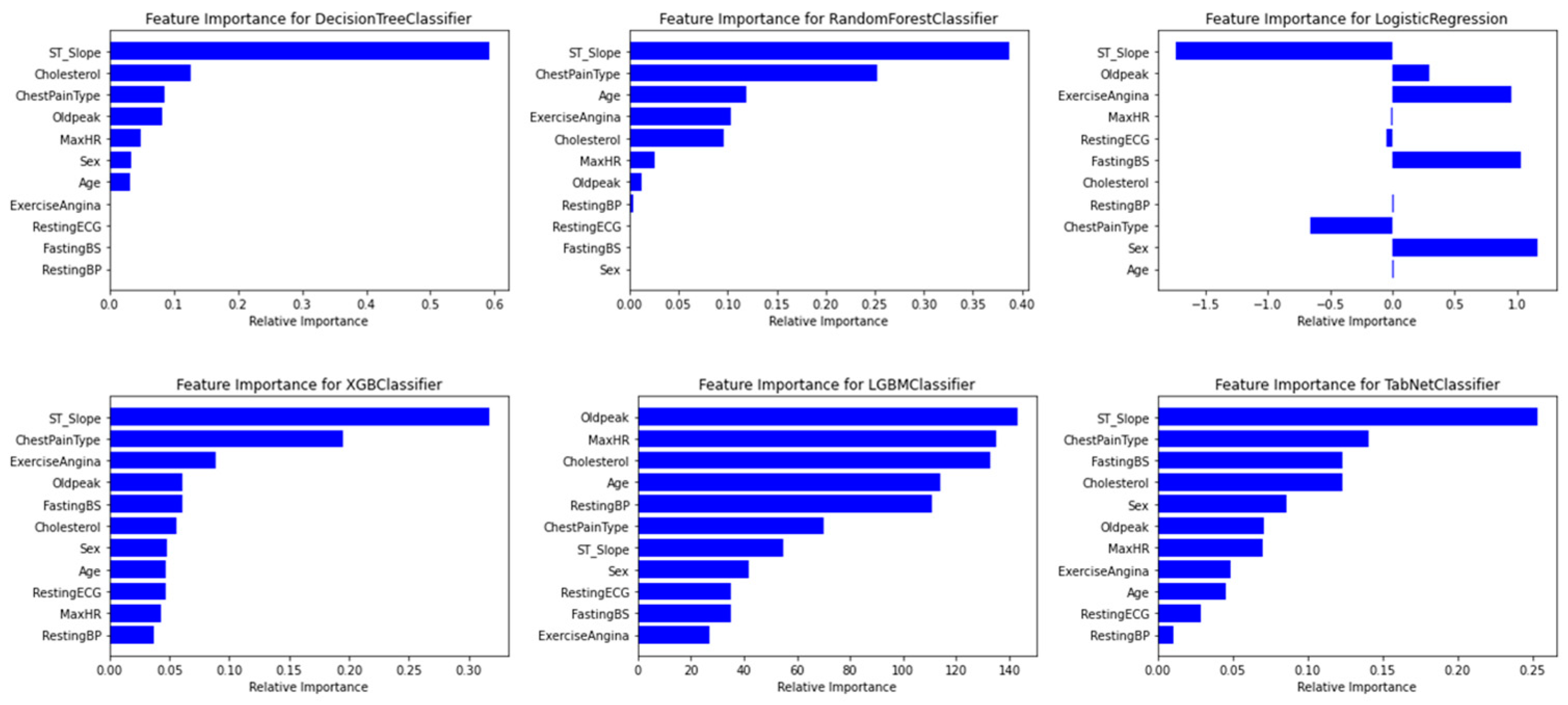
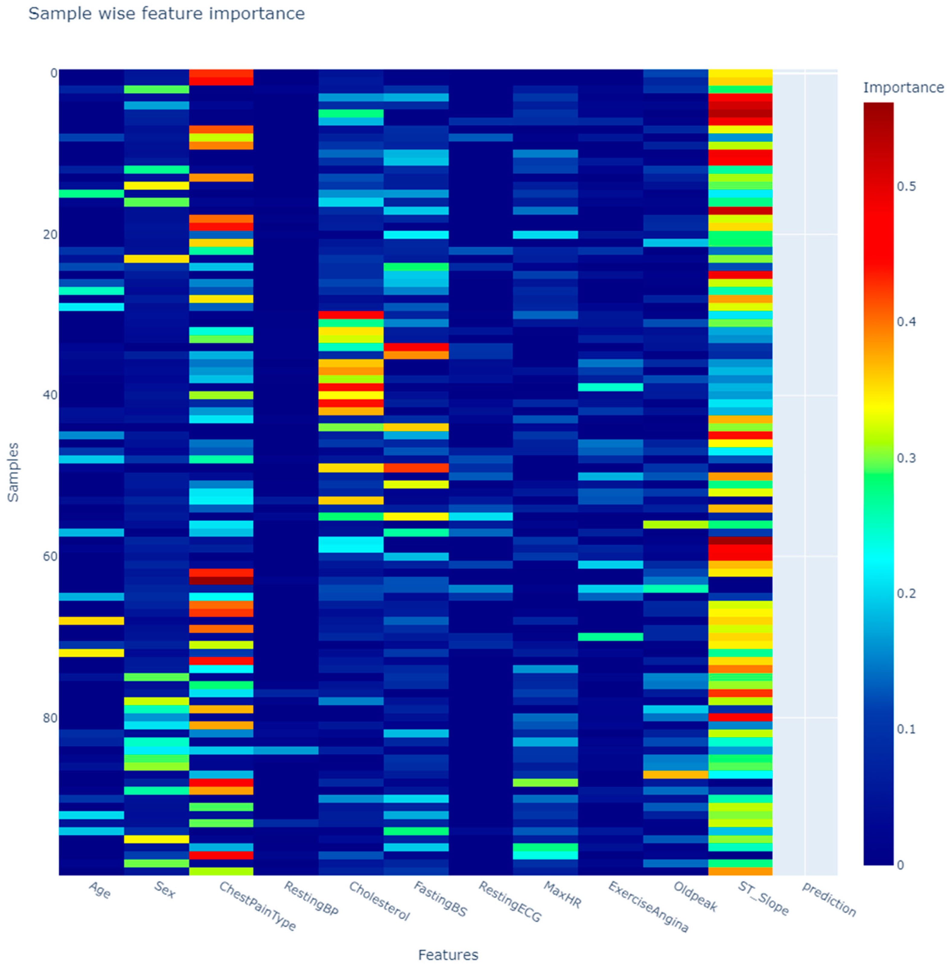
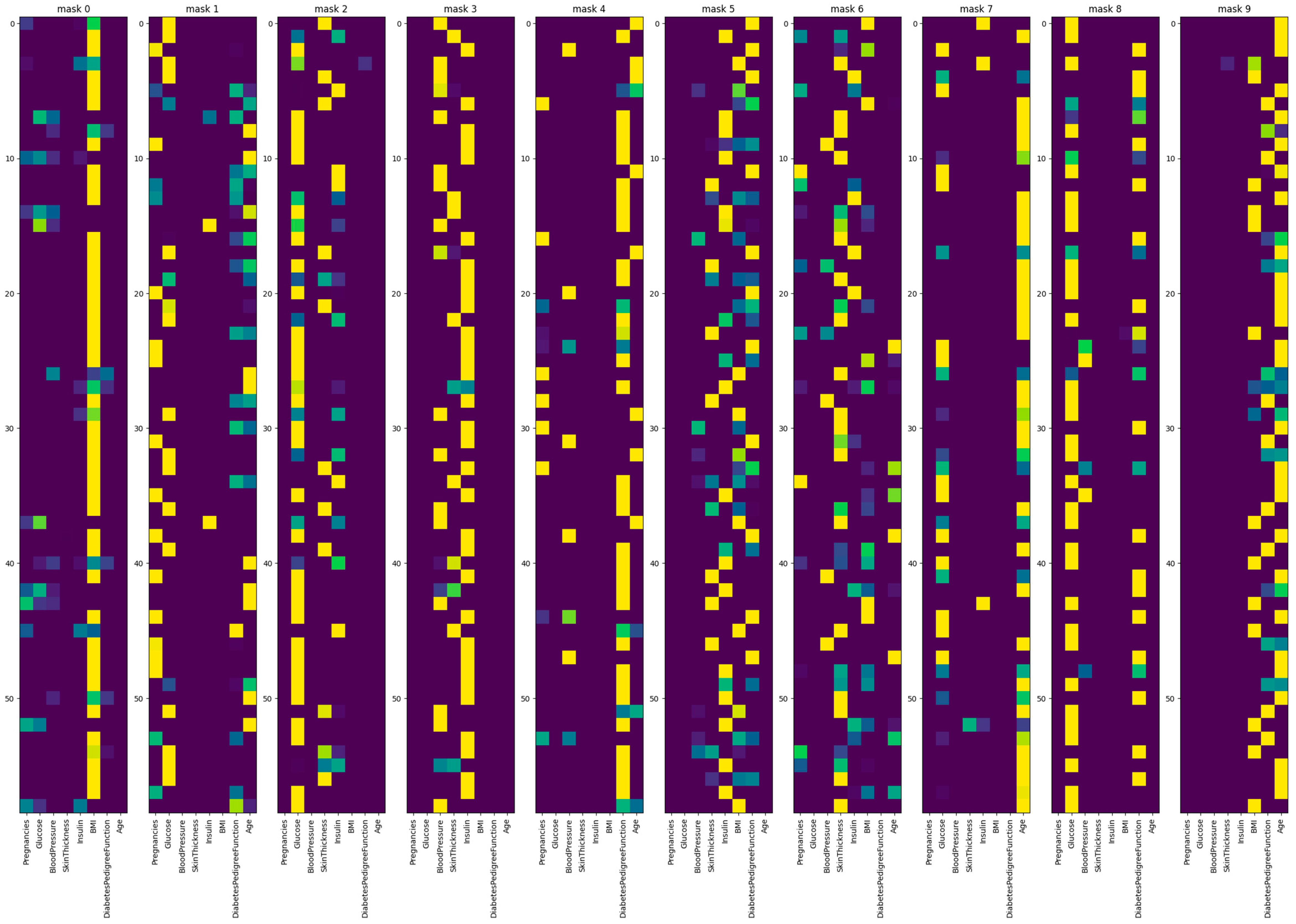
This study aimed to address the question of how to effectively select an optimal explainer to reduce misinterpretations. The study evaluated various classification models with a focus on recall across two medical tabular datasets. In both studies, XGBoost emerged as the top-performing model for classification and explainability tasks. This is followed by TabNet and TabPFN. A notable strength of utilizing TabNet lies in its model-specific explainability and capability to inject additional knowledge into the model. While TabPFN demonstrated satisfactory performance, it comprises multiple challenges within the scope of explainability including the lack of built-in model-specific interpretability struggles with providing feature importance, and incompatibility with the majority of model-agnostic explainers due to its black-box nature and time-consuming process. Furthermore, the study examined the intrinsic feature importance of these models. The result demonstrates a consensus with XGboost, LightGBM, and TabNet. Additionally, DT, RF, and LR are unsuccessful in generating reasonable logic as they failed to capture the correct feature relations in both studies.

In addition, the study utilized LIME, SHAP, and Anchors to generate explanations. Consequently, LIME stands out as the most unstable model specifically at the local level, endangering user trust. In LIME explanations, TabNet and TabPFN identified similar behaviors, however, they represent different prediction probabilities in many test cases. In addition, TabNet displayed unique behavior in comparison to all models. DT and RF were found to pose a higher risk of misinterpretations across all techniques, which is not surprising based on their unreasonable behavior from global feature importance. XGBoost maintained a consistent ranking for certain features, with slight differences. Anchors consistently demonstrated the highest precision across all models within both experiments. However, Anchors represent significantly less coverage for the second dataset.

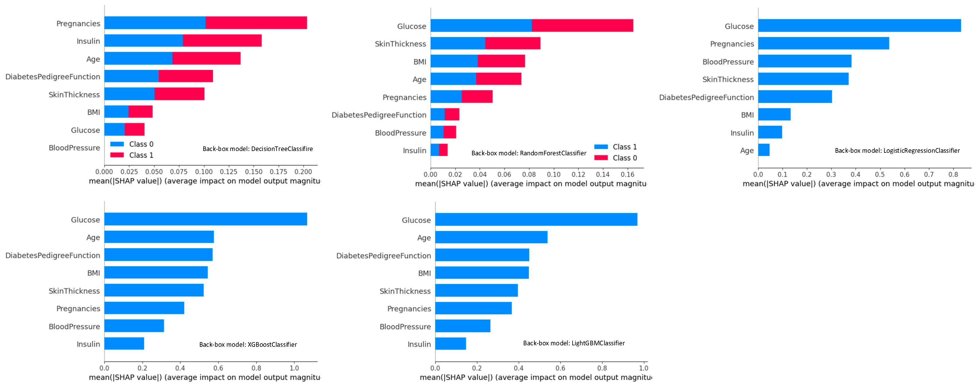
In addition, this study compared global feature importance across different techniques, including intrinsic and post-hoc model explainability at the global level. This resulted in a varying feature importance ranking for each technique. The results derived from both experiments, model-agnostic explanations including SHAP, and LIME exhibit similar behavior for XGBoost and LightGBM. However, model-specific explainers, particularly TabNet in this study, demonstrate advanced precision in explaining the decision. Across both studies, DT is recognized as the least-performing model due to its inaccuracies in either eliminating necessary features or learning the incorrect feature relations. In contrast, there was no consensus on the topmost important features of RF and LR across all four techniques. This disparity resulted because intrinsic model explanations rely on impurity-based feature importance, which is based on differences in entropy whereas LIME uses linear model coefficients, and SHAP aggregates Shapley values [65] across all instances [4,13,66]. On the contrary, feature contributions obtained from the interpretable ensemble models were incorporated into the models as part of their optimization process. These interpretabilities are directly incorporated from model structure whereas post-hoc model-agnostic explanations are limited in their strength in approximating the black box. Their key difference lies in the trade-off between model accuracy and explanation fidelity [67].

Our study underscores the consistency in feature importance with certain findings across the literature. As an example, our results aligned with the research conducted by Tasin et al. (2022), where LIME and SHAP were employed as their explainer, identifying XGBoost as the best-performing model. Remarkably, Glucose, BMI, and Age were recognized as the most salient features [68]. Similarly, another study employed similar methods including RF and XGBoost, and employed LIM and SHAP as explainers [69].

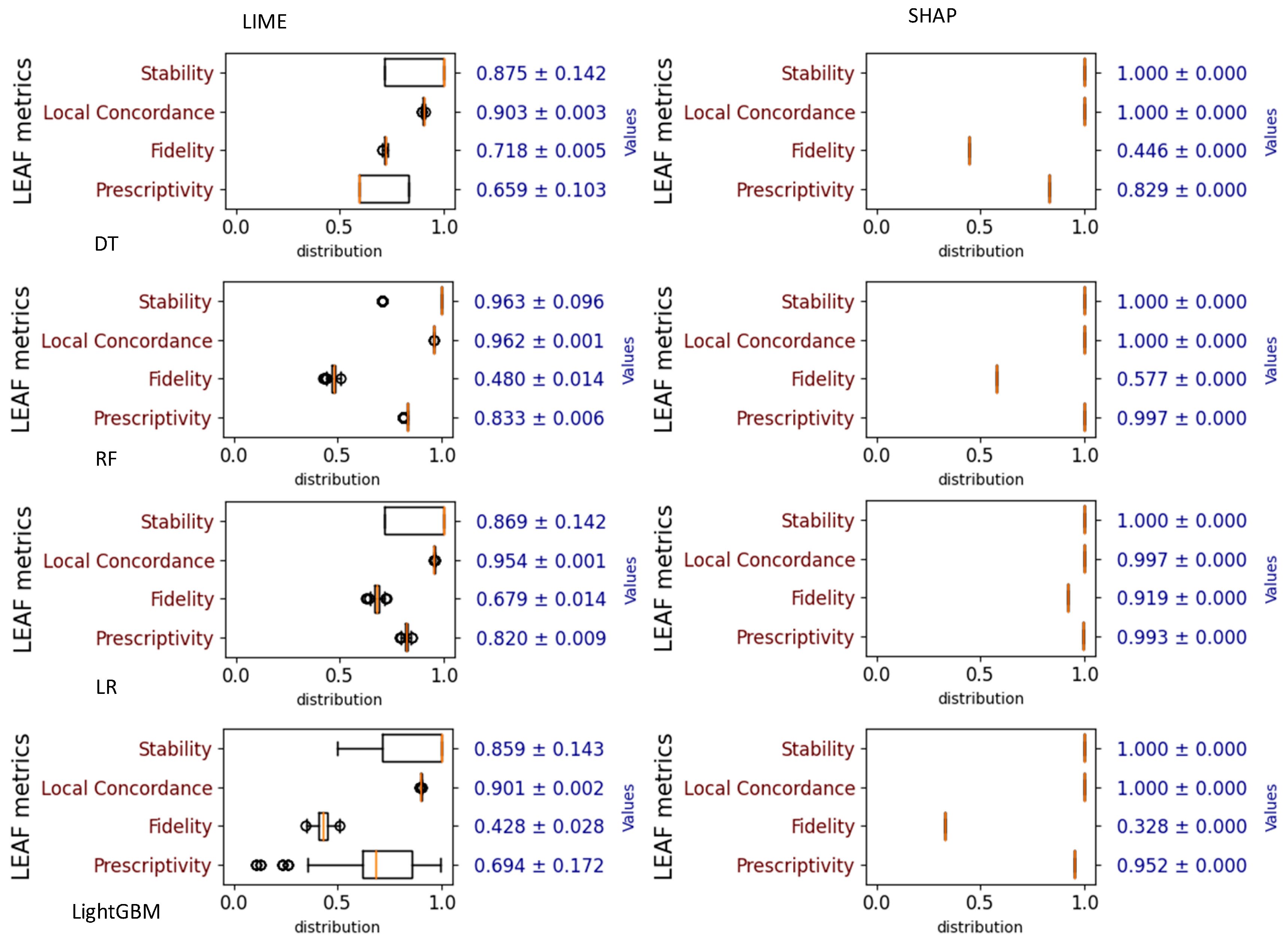
LEAF was employed to evaluate the explainers at the local level. Subsequently, LIME achieved the best stability with LightGBM, with the highest local concordance score for LR and the best prescriptivity for RF for the heart disease dataset and best stability with RF, the highest local concordance with RF and LR, and the best prescriptivity with RF. However, LIME performed poorly in terms of fidelity, with slightly better results for RF for the first dataset whereas for the second one, SHAP is identified with the lowest fidelity score, except for LR with a fidelity of 0.91. In general, SHAP demonstrates better performance with optimal stability, local concordance, and presciptivity across all models.

In evaluating global feature importance for a classification, this study recommends Relative Performance Loss as a metric that calculates the impact of global feature contributions on model loss. As a result, XGBoost demonstrates excellent compatibility with all three model-agnostic explainers within both experiments. In the first experiment, DT and LightGBM performed best with Anchors, RF with SHAP, and LR with LIME. Furthermore, TabNet demonstrates the most effective global feature importance, followed by XGBoost and TabPFN. For the second dataset, the best explainer is devoted to XGBoost with the best results across all explainers, this choice is followed by TabNet and TabPFN.

10. Discussion of Algorithm Selection

Machine learning algorithms have shown impressive performance in various domains, especially in medicine. However, these algorithms are often seen as complex black boxes that lack transparency, which poses a challenge to trust among clinicians. To address this, numerous XAI frameworks have been proposed to shed light on their inner logic. The enormous XAI frameworks, along with their misinterpreting risk, have grown as a need for assessing these explainers. Consequently, a significant portion of the literature focuses on developing new evaluation frameworks. However, the diversity of topics within the XAI literature led to a lack of consensus, making it difficult to choose the optimal approach. This study contributed to the field of XAI by introducing some unity by proposing a framework to assist in choosing an explainer.

The result, this study identified XGboost, TabNet, and TabPFN as optimal models by initially evaluating at the global level utilizing relative performance loss, followed by local evaluation using LEAF. The result indicates SHAP with superior stability and local concordance, with optimal fidelity and perceptivity for LR which is aligned with the result conducted by [56].

This study addresses the question of how to arrive at the best explainers for classification involving tabular data by proposing a three-layered top-down approach. First, it emphasizes the importance of identifying the application domain and considering the end-user experience. As an example, it is incredibly important for a user to be able to understand the explanations otherwise the interpretability might be damaged. Different applications require different criteria of sensitivity and completeness. Time limitation is another crucial factor. Extremely sensitive tasks such as disease diagnoses require appropriate time to understand the explanations and explore the patient’s history and disease etiology. Complexity is another criterion that indicates whether explanations need to be comprehensive or selective. Lastly, the social/interactivity aspects of explanations can be useful in specific domains, facilitating user communication with the framework.

Following the initial assessment and selecting techniques for specific application domains, the study signifies evaluating global explanations before local level evaluation. Global explanations assess the overall behavior of the algorithm, whereas local explanations are limited to the scope of individual instances and provide fewer insights into model behavior. To be concise, the study suggests applying relative loss performance to evaluate the global explanations to assess their feature contribution impact on model loss by feature pruning. The results yield an overall insight into model behavior and evaluate the model’s capability in choosing relevant features. This algorithm is outstanding because it is agnostic to both model and explainer and can be applied to any classification task. The insight from this approach leads to possible explainers that are globally accurate and select relevant features.

Subsequently, the study advocates conducting local evaluations to qualify individual explanations. High-quality global explanations ensure the quality of local explanations [13]. The top-down approach is illustrated in Figure 1, arrives at optimal explanations for specific tasks. There are many approaches to evaluating local explanations. This study makes use of the LEAF. Quantus and OpenXA are other alternatives recommended for future work.

11. Limitations

To gain a comprehensive understanding of our findings, it is crucial to consider the limitations inherent in this study. Limited literature developed deep neural model-specific explanations capable of interpreting the result at both global and local level. This study utilized TabNet and TabPFN for their popularity in outperforming XGBoost. A similar limitation arises in XAI explainers. This research utilized SHAP, LIME, Anchors, and TabNet because of their established performance in working with such applications. The gap increases in XAI evaluation as it is a newly explored field of study, stressing limited work around it. LEAF happened to be useful but is only functional for local linear models and SHAP and LIME explainers. Subsequently, it is not suitable for XGBoost and Anchors. Another limitation is that most of the explainability criteria introduced in the literature suffer from consistent and concise definitions and lack of implementation. The researchers address this gap by developing a framework for calculating log loss relative performance. Another limitation arises from TabPFN, because of its lack of intrinsic explainability, or global feature importance, and due to its time-consuming and rigid nature in applying with multiple explainers was challenging. In addition, however slow, the eli5 library was also useful in generating global explainability for TabPFN.

Moreover, this study confines its evaluation around the impact of global and local explanations and does not consider other forms of explanations such as counterfactual explanations. Future work is recommended to expand the work by considering an extensive range of explainability methods. In addition, the current investigation is specifically tailored around tabular. This is driven by the limited work around the tabular data in the literature. In addition, the majority of the data, especially in medical, is intrinsically tabular. However, the authors recommend expanding this work in different data domains such as images, text, etc., and different areas such as finance, criminal justice, weather forecast etc., to extreme investigation of the evaluation methodology.

12. Conclusions and Future Work

This paper has aimed to examine the relevant literature for the field of explainability evaluation and arrive at a conclusion on which approaches to consider when adding XAI to AI-system. This work has combined various approaches to conduct a comparative evaluation of techniques used across literature. In evaluating the explainers applied in the study, the research contributed to gathering relevant work on literature to converge on the most important criteria, then the study proposed relative performance loss as the metric to evaluate global explainability. One positive contribution of this study is that even though the research has focused on the classification task, the three-layered top-down approach can be considered for all applications as it generally evaluates the important principles prioritized sequentially, and the metrics themselves, such as loss can be tailored for a specific task. For classification, this study has contributed to the relative performance evaluation of log loss. The contribution of this research is accomplished as a guideline for evaluating whether the explainers should be trusted. Performance measurement in the context of XAI is a challenging task. Multiple explanations and application criteria such as fidelity, complexity, selectivity, etc. must be considered which are discussed in the study. The novelty of this study is to combine both qualitative and quantitative methods. The main goal of such XAI frameworks is to eliminate the human in the decision loop due to many reasons including limited access to domain experts in multiple scenarios, time-sensitivity of the task, or increasing the precision and to allow XAI to explain itself to end-users. However, for a highly sensitive task such as medical, XAI requires domain supervision which is included in the first layer of this framework. Even in this case, the XAI will assist medical practitioners to enhance their precision and reduce misinterpretation in the decision-making process.

On the concept of improving user trust, several studies have argued that adding the calibration layer has a significant effect on improving the quality of explanations, therefore, increasing user trust. The research conducted by Scafarto, Posocco, and Bonnefoy [70] on image data demonstrates that post-hoc calibration can positively impact the quality of saliency maps in terms of faithfulness, stability, and visual coherence. In addition, the authors argue that applying the calibration before interpretability will lead to more trustworthy and accurate explanations. Another study by Mohammad Naiseh et al. [71] explored four different explainability methods including local, example-based, counterfactual, and global explanations during human-AI collaborative decision-making tasks to investigate how different explanations impact trust calibration in clinical decision-making. Their work highlighted that local explanations are more efficient in explaining unfair model decisions and, therefore, more beneficial in calibrating the user fairness judgment. In addition, they argue that including the confidence score enhances the user’s trust calibration. As a result of their study, example-based and counterfactual explanations were more interpretable than others. Moreover, the study conducted by Zhang, Liao, and Bellamy [72] supports the idea that including confidence score in end-users decision-making- process will positively impact the trust calibration. The major findings of the study argue that local explanations significantly improve user trust and AI accuracy even more than confidence score. The main study by Löfström et al. [73] investigates the impacts of the calibration in the explanation quality by utilizing misleading explainers such as LIME. The study indicates that adding a layer of calibration will significantly enhance the accuracy and fidelity of explanations. In the experiment with LIME, a well-calibrated black-box model will lead to well-calibrated explanations. They also argue that for a poorly calibrated model, the confidence score may not reflect true probabilities, leading to misinterpretations. In addition, in a poorly calibrated model, the explanations produce a higher log loss, indicating the larger errors by the explanations. The calibration layer will assist in ensuring that the model’s confidence is aligned with its accuracy. To improve calibration, their study employed Platt scaling and Venn–Abers. However, Venn–Abers is considered the optimal choice. Another framework was developed by Famiglini, Campagner, and Cabitza [74] to assess the calibration. Therefore, based on the recent study and the positive and required effect of calibration, the focus is on further investigating the effect of calibration within the framework by adding a layer of calibration evaluation and re-calibration to the pipeline before explanations and evaluating the quality of explanations to deeper investigate the XAI evaluation.

In addition, since the requirements of medical AI systems are different, special attention must be given to models that can process medical applications based on their specific criteria. A future might benefit from XAI explainers that are more detailed and perform along with human logic systems in order to be trusted within the medical community. Extracting the strengths and weaknesses of each explainer will assist in detecting the gap in developing enhanced explainers, therefore, developing a more accurate framework. The future work must be aware to provide evaluations that are capable of evaluating various explainers. Moreover, the techniques proposed in this paper will benefit from further enhancement in future work by examining various datasets across various domains. For this reason, the research emphasizes the importance of future work in expanding this work in various approaches.

References

1. Karim, M.R.; Islam, T.; Beyan, O.; Lange, C.; Cochez, M.; Rebholz-Schuhmann, D.; Decker, S. Explainable AI for Bioinformatics: Methods, Tools, and Applications. arXiv 2022, arXiv:2212.13261. [Google Scholar] [CrossRef] [PubMed]
2. Saeed, W.; Omlin, C. Explainable AI (XAI): A Systematic Meta-Survey of Current Challenges and Future Opportunities. Knowl. Based Syst. 2023, 263, 110273. [Google Scholar] [CrossRef]
3. Stassin, S.; Englebert, A.; Nanfack, G.; Albert, J.; Versbraegen, N.; Peiffer, G.; Doh, M.; Riche, N.; Frenay, B.; De Vleeschouwer, C. An Experimental Investigation into the Evaluation of Explainability Methods. arXiv 2023, arXiv:2305.16361. [Google Scholar]
4. Ribeiro, M.T.; Singh, S.; Guestrin, C. “Why Should I Trust You?” Explaining the Predictions of Any Classifier. In Proceedings of the 22nd ACM SIGKDD International Conference on Knowledge Discovery and Data Mining, New York, NY, USA, 13–17 August 2016; pp. 1135–1144. [Google Scholar]
5. Liao, Q.V.; Zhang, Y.; Luss, R.; Doshi-Velez, F.; Dhurandhar, A. Connecting Algorithmic Research and Usage Contexts: A Perspective of Contextualized Evaluation for Explainable AI. In Proceedings of the AAAI Conference on Human Computation and Crowdsourcing, Virtual, 6–10 November 2022; Volume 10, pp. 147–159. [Google Scholar]
6. Carvalho, D.V.; Pereira, E.M.; Cardoso, J.S. Machine Learning Interpretability: A Survey on Methods and Metrics. Electronics 2019, 8, 832. [Google Scholar] [CrossRef]
7. Papenmeier, A.; Englebienne, G.; Seifert, C. How Model Accuracy and Explanation Fidelity Influence User Trust. arXiv 2019, arXiv:1907.12652. [Google Scholar]
8. Dieber, J.; Kirrane, S. A Novel Model Usability Evaluation Framework (MUsE) for Explainable Artificial Intelligence. Inf. Fusion. 2022, 81, 143–153. [Google Scholar] [CrossRef]
9. Duell, J.; Fan, X.; Burnett, B.; Aarts, G.; Zhou, S.-M. A Comparison of Explanations given by Explainable Artificial Intelligence Methods on Analysing Electronic Health Records. In Proceedings of the 2021 IEEE EMBS International Conference on Biomedical and Health Informatics (BHI), Athens, Greece, 27–30 July 2021; IEEE: Piscataway, NJ, USA, 2021; pp. 1–4. [Google Scholar]
10. Zhang, Y.; Xu, F.; Zou, J.; Petrosian, O.L.; Krinkin, K.V. XAI Evaluation: Evaluating Black-Box Model Explanations for Prediction. In Proceedings of the 2021 II International Conference on Neural Networks and Neurotechnologies (NeuroNT), Saint Petersburg, Russia, 16 June 2021; IEEE: Piscataway, NJ, USA, 2021; pp. 13–16. [Google Scholar]
11. Arik, S.Ö.; Pfister, T. Tabnet: Attentive Interpretable Tabular Learning. In Proceedings of the AAAI Conference on Artificial Intelligence, Virtual, 2–9 February 2021; Volume 35, pp. 6679–6687. [Google Scholar]
12. Hollmann, N.; Müller, S.; Eggensperger, K.; Hutter, F. Tabpfn: A Transformer That Solves Small Tabular Classification Problems in a Second. arXiv 2022, arXiv:2207.01848. [Google Scholar]
13. Lundberg, S.M.; Lee, S.-I. A Unified Approach to Interpreting Model Predictions. Adv. Neural Inf. Process Syst. 2017, 30. [Google Scholar] [CrossRef]
14. Ribeiro, M.T.; Singh, S.; Guestrin, C. Anchors: High-Precision Model-Agnostic Explanations. In Proceedings of the AAAI Conference on Artificial Intelligence, New Orleans, LA, USA, 2–7 February 2018; Volume 32. [Google Scholar]
15. Scapin, D.; Cisotto, G.; Gindullina, E.; Badia, L. Shapley Value as an Aid to Biomedical Machine Learning: A Heart Disease Dataset Analysis. In Proceedings of the 2022 22nd IEEE International Symposium on Cluster, Cloud and Internet Computing (CCGrid), Taormina, Italy, 16–19 May 2022; IEEE: Piscataway, NJ, USA, 2022; pp. 933–939. [Google Scholar]
16. Gurgul, J.; Paździerz, A.; Wydra, D. A Parameters-Based Heart Disease Prediction Model. Age 2022, 53, 28. [Google Scholar]
17. Bhatt, C.M.; Patel, P.; Ghetia, T.; Mazzeo, P.L. Effective Heart Disease Prediction Using Machine Learning Techniques. Algorithms 2023, 16, 88. [Google Scholar] [CrossRef]
18. Bakar, W.A.W.A.; Josdi, N.L.N.B.; Man, M.B.; Zuhairi, M.A.B. A Review: Heart Disease Prediction in Machine Learning & Deep Learning. In Proceedings of the 2023 19th IEEE International Colloquium on Signal Processing & Its Applications (CSPA), Kedah, Malaysia, 3–4 March 2023; IEEE: Piscataway, NJ, USA, 2023; pp. 150–155. [Google Scholar]
19. Dileep, P.; Rao, K.N.; Bodapati, P.; Gokuruboyina, S.; Peddi, R.; Grover, A.; Sheetal, A. An Automatic Heart Disease Prediction Using Cluster-Based Bi-Directional LSTM (C-BiLSTM) Algorithm. Neural Comput. Appl. 2023, 35, 7253–7266. [Google Scholar] [CrossRef]
20. Narayan, V.; Mall, P.K.; Alkhayyat, A.; Abhishek, K.; Kumar, S.; Pandey, P. Enhance-Net: An Approach to Boost the Performance of Deep Learning Model Based on Real-Time Medical Images. J. Sens. 2023, 2023, 8276738. [Google Scholar] [CrossRef]
21. Sun, B.; Yang, L.; Zhang, W.; Lin, M.; Dong, P.; Young, C.; Dong, J. Supertml: Two-Dimensional Word Embedding for the Precognition on Structured Tabular Data. In Proceedings of the IEEE/CVF Conference on Computer Vision and Pattern Recognition Workshops, Long Beach, CA, USA, 16–17 June 2019. [Google Scholar]
22. Liu, G.; Yang, J.; Wu, L. PTab: Using the Pre-Trained Language Model for Modeling Tabular Data. arXiv 2022, arXiv:2209.08060. [Google Scholar]
23. Wang, Z.; Sun, J. Transtab: Learning Transferable Tabular Transformers across Tables. Adv. Neural Inf. Process Syst. 2022, 35, 2902–2915. [Google Scholar]
24. Kadiyala, S.P.; Woo, W.L. Flood Prediction and Analysis on the Relevance of Features using Explainable Artificial Intelligence. In Proceedings of the 2021 2nd Artificial Intelligence and Complex Systems Conference, Bangkok, Thailand, 21–22 October 2021; 2021; pp. 1–6. [Google Scholar] [CrossRef]
25. Sanderson, J.; Tengtrairat, N.; Woo, W.L.; Mao, H.; Al-Nima, R.R. XFIMNet: An Explainable Deep Learning Architecture for Versatile Flood Inundation Mapping with Synthetic Aperture Radar and Multi-Spectral Optical Images. Int. J. Remote Sens. 2023, 44, 7755–7789. [Google Scholar] [CrossRef]
26. Lagioia, F. The Impact of the General Data Protection Regulation (GDPR) on Artificial Intelligence; European Parliamentary Research Service: Brussels, Belgium, 2020. [Google Scholar]
27. Sahakyan, M.; Aung, Z.; Rahwan, T. Explainable Artificial Intelligence for Tabular Data: A Survey. IEEE Access 2021, 9, 135392–135422. [Google Scholar] [CrossRef]
28. Plumb, G.; Molitor, D.; Talwalkar, A.S. Model Agnostic Supervised Local Explanations. Adv. Neural Inf. Process Syst. 2018, 31. [Google Scholar] [CrossRef]
29. Selvaraju, R.R.; Cogswell, M.; Das, A.; Vedantam, R.; Parikh, D.; Batra, D. Grad-Cam: Visual Explanations from Deep Networks via Gradient-Based Localization. In Proceedings of the IEEE International Conference on Computer Vision, Venice, Italy, 22–29 October 2017; pp. 618–626. [Google Scholar]
30. Lakkaraju, H.; Kamar, E.; Caruana, R.; Leskovec, J. Faithful and Customizable Explanations of Black Box Models. In Proceedings of the 2019 AAAI/ACM Conference on AI, Ethics, and Society, Honolulu, HI, USA, 27–28 January 2019; pp. 131–138. [Google Scholar]
31. Dieber, J.; Kirrane, S. Why Model Why? Assessing the Strengths and Limitations of LIME. arXiv 2020, arXiv:2012.00093. [Google Scholar]
32. Montavon, G.; Binder, A.; Lapuschkin, S.; Samek, W.; Müller, K.-R. Layer-Wise Relevance Propagation: An Overview. Explainable AI: Interpreting, Explaining and Visualizing Deep Learning; Springer International Publishing: Berlin/Heidelberg, Germany, 2019; pp. 193–209. [Google Scholar]
33. Grezmak, J.; Zhang, J.; Wang, P.; Loparo, K.A.; Gao, R.X. Interpretable Convolutional Neural Network through Layer-Wise Relevance Propagation for Machine Fault Diagnosis. IEEE Sens. J. 2019, 20, 3172–3181. [Google Scholar] [CrossRef]
34. Mandloi, S.; Zuber, M.; Gupta, R.K. An Explainable Brain Tumor Detection and Classification Model Using Deep Learning and Layer-Wise Relevance Propagation. Multimed. Tools Appl. 2023, 1–31. [Google Scholar] [CrossRef]
35. Hassan, M.M.; AlQahtani, S.A.; Alelaiwi, A.; Papa, J.P. Explaining COVID-19 Diagnosis with Taylor Decompositions. Neural Comput. Appl. 2023, 35, 22087–22100. [Google Scholar] [CrossRef] [PubMed]
36. Clement, T.; Kemmerzell, N.; Abdelaal, M.; Amberg, M. XAIR: A Systematic Metareview of Explainable AI (XAI) Aligned to the Software Development Process. Mach. Learn. Knowl. Extr. 2023, 5, 78–108. [Google Scholar] [CrossRef]
37. Thien, T.Q. Concept and Pattern Discovery for Reliable and Explainable AI. PhD Thesis, University of Tsukuba, Tsukuba, Japan.
38. Sreekumar, G.; Boddeti, V.N. Spurious Correlations and Where to Find Them. arXiv 2023, arXiv:2308.11043. [Google Scholar]
39. Fan, J.; Han, F.; Liu, H. Challenges of Big Data Analysis. Natl. Sci. Rev. 2014, 1, 293–314. [Google Scholar] [CrossRef] [PubMed]
40. Lapuschkin, S.; Wäldchen, S.; Binder, A.; Montavon, G.; Samek, W.; Müller, K.-R. Unmasking Clever Hans Predictors and Assessing What Machines Really Learn. Nat. Commun. 2019, 10, 1096. [Google Scholar] [CrossRef] [PubMed]
41. Hailemariam, Y.; Yazdinejad, A.; Parizi, R.M.; Srivastava, G.; Dehghantanha, A. An Empirical Evaluation of AI Deep Explainable Tools. In Proceedings of the 2020 IEEE Globecom Workshops (GC Wkshps), Taipei, Taiwan, 7–11 December 2020; IEEE: Piscataway, NJ, USA, 2020; pp. 1–6. [Google Scholar]
42. Burger, C.; Chen, L.; Le, T. Are Your Explanations Reliable? Investigating the Stability of LIME in Explaining Textual Classification Models via Adversarial Perturbation. arXiv 2023, arXiv:2305.12351. [Google Scholar]
43. Fel, T.; Hervier, L.; Vigouroux, D.; Poche, A.; Plakoo, J.; Cadene, R.; Chalvidal, M.; Colin, J.; Boissin, T.; Béthune, L. Xplique: A Deep Learning Explainability Toolbox. arXiv 2022, arXiv:2206.04394. [Google Scholar]
44. Simonyan, K.; Vedaldi, A.; Zisserman, A. Deep inside Convolutional Networks: Visualising Image Classification Models and Saliency Maps. arXiv 2013, arXiv:1312.6034. [Google Scholar]
45. Schwegler, M.; Müller, C.; Reiterer, A. Integrated Gradients for Feature Assessment in Point Cloud-Based Data Sets. Algorithms 2023, 16, 316. [Google Scholar] [CrossRef]
46. Biecek, P. DALEX: Explainers for Complex Predictive Models in R. J. Mach. Learn. Res. 2018, 19, 3245–3249. [Google Scholar]
47. Kuhn, M. Building Predictive Models in R Using the Caret Package. J. Stat. Softw. 2008, 28, 1–26. [Google Scholar] [CrossRef]
48. Greenwell, B.M. Pdp: An R Package for Constructing Partial Dependence Plots. R. J. 2017, 9, 421. [Google Scholar] [CrossRef]
49. Apley, D.W.; Zhu, J. Visualizing the effects of predictor variables in black box supervised learning models. J. R. Stat. Soc. Ser. B Stat. Methodol. 2020, 82, 1059–1086. [Google Scholar] [CrossRef]
50. Sitko, A.; Biecek, P. The Merging Path Plot: Adaptive Fusing of k-Groups with Likelihood-Based Model Selection. arXiv 2017, arXiv:1709.04412. [Google Scholar]
51. Arya, V.; Bellamy, R.K.E.; Chen, P.-Y.; Dhurandhar, A.; Hind, M.; Hoffman, S.C.; Houde, S.; Liao, Q.V.; Luss, R.; Mojsilović, A. One Explanation Does Not Fit All: A Toolkit and Taxonomy of Ai Explainability Techniques. arXiv 2019, arXiv:1909.03012. [Google Scholar]
52. Klaise, J.; Van Looveren, A.; Vacanti, G.; Coca, A. Alibi Explain: Algorithms for Explaining Machine Learning Models. J. Mach. Learn. Res. 2021, 22, 8194–8200. [Google Scholar]
53. Hedström, A.; Weber, L.; Krakowczyk, D.; Bareeva, D.; Motzkus, F.; Samek, W.; Lapuschkin, S.; Höhne, M.M.-C. Quantus: An Explainable Ai Toolkit for Responsible Evaluation of Neural Network Explanations and Beyond. J. Mach. Learn. Res. 2023, 24, 1–11. [Google Scholar]
54. Agarwal, C.; Krishna, S.; Saxena, E.; Pawelczyk, M.; Johnson, N.; Puri, I.; Zitnik, M.; Lakkaraju, H. Openxai: Towards a Transparent Evaluation of Model Explanations. Adv. Neural Inf. Process Syst. 2022, 35, 15784–15799. [Google Scholar]
55. Belaid, M.K.; Hüllermeier, E.; Rabus, M.; Krestel, R. Do We Need Another Explainable AI Method? Toward Unifying Post-Hoc XAI Evaluation Methods into an Interactive and Multi-Dimensional Benchmark. arXiv 2022, arXiv:2207.14160. [Google Scholar]
56. Amparore, E.; Perotti, A.; Bajardi, P. To Trust or Not to Trust an Explanation: Using LEAF to Evaluate Local Linear XAI Methods. PeerJ Comput. Sci. 2021, 7, e479. [Google Scholar] [CrossRef]
57. Bischl, B.; Binder, M.; Lang, M.; Pielok, T.; Richter, J.; Coors, S.; Thomas, J.; Ullmann, T.; Becker, M.; Boulesteix, A. Hyperparameter Optimization: Foundations, Algorithms, Best Practices, and Open Challenges. Wiley Interdiscip. Rev. Data Min. Knowl. Discov. 2023, 13, e1484. [Google Scholar] [CrossRef]
58. Turner, R.; Eriksson, D.; McCourt, M.; Kiili, J.; Laaksonen, E.; Xu, Z.; Guyon, I. Bayesian Optimization Is Superior to Random Search for Machine Learning Hyperparameter Tuning: Analysis of the Black-Box Optimization Challenge 2020. In Proceedings of the NeurIPS 2020 Competition and Demonstration Track, PMLR, Virtual, 6–12 December 2020; pp. 3–26. [Google Scholar]
59. Molnar, C. Interpretable Machine Learning: A Guide for Making Black Box Models Interpretable; Lulu: Morisville, NC, USA, 2019. [Google Scholar]
60. Salih, A.; Raisi-Estabragh, Z.; Galazzo, I.B.; Radeva, P.; Petersen, S.E.; Menegaz, G.; Lekadir, K. Commentary on Explainable Artificial Intelligence Methods: SHAP and LIME. arXiv 2023, arXiv:2305.02012. [Google Scholar]
61. Guidotti, R.; Monreale, A.; Ruggieri, S.; Turini, F.; Giannotti, F.; Pedreschi, D. A Survey of Methods for Explaining Black Box Models. ACM Comput. Surv. (CSUR) 2018, 51, 1–42. [Google Scholar] [CrossRef]
62. Heart Failure Prediction Dataset. Available online: https://www.kaggle.com/datasets/fedesoriano/heart-failure-prediction (accessed on 30 September 2023).
63. PIMA Indian Dataset. Available online: https://www.kaggle.com/datasets/uciml/pima-indians-diabetes-database (accessed on 13 December 2023).
64. Chawla, N.V.; Bowyer, K.W.; Hall, L.O.; Kegelmeyer, W.P. SMOTE: Synthetic Minority over-Sampling Technique. J. Artif. Intell. Res. 2002, 16, 321–357. [Google Scholar] [CrossRef]
65. Kuhn, H.W.; Tucker, A.W. Contributions to the Theory of Games; Princeton University Press: Princeton, NJ, USA, 1953. [Google Scholar]
66. Ensembles: Gradient Boosting, Random Forests, Bagging, Voting, Stacking—Scikit-Learn 1.3.1 Documentation. Available online: https://scikit-learn.org/stable/modules/ensemble.html (accessed on 30 September 2023).
67. Du, M.; Liu, N.; Hu, X. Techniques for Interpretable Machine Learning. Commun. ACM 2019, 63, 68–77. [Google Scholar] [CrossRef]
68. Tasin, I.; Nabil, T.U.; Islam, S.; Khan, R. Diabetes Prediction Using Machine Learning and Explainable AI Techniques. Healthc. Technol. Lett. 2023, 10, 1–10. [Google Scholar] [CrossRef]
69. Kibria, H.B.; Nahiduzzaman, M.; Goni, M.O.F.; Ahsan, M.; Haider, J. An Ensemble Approach for the Prediction of Diabetes Mellitus Using a Soft Voting Classifier with an Explainable AI. Sensors 2022, 22, 7268. [Google Scholar] [CrossRef]
70. Scafarto, G.; Posocco, N.; Bonnefoy, A. Calibrate to Interpret. In Proceedings of the Joint European Conference on Machine Learning and Knowledge Discovery in Databases, Grenoble, France, 19–23 September 2022; Springer: Berlin/Heidelberg, Germany, 2022; pp. 340–355. [Google Scholar]
71. Naiseh, M.; Al-Thani, D.; Jiang, N.; Ali, R. How the Different Explanation Classes Impact Trust Calibration: The Case of Clinical Decision Support Systems. Int. J. Hum. Comput. Stud. 2023, 169, 102941. [Google Scholar] [CrossRef]
72. Zhang, Y.; Liao, Q.V.; Bellamy, R.K.E. Effect of Confidence and Explanation on Accuracy and Trust Calibration in AI-Assisted Decision Making. In Proceedings of the 2020 Conference on Fairness, Accountability, and Transparency, Barcelona, Spain, 27–30 January 2020; pp. 295–305. [Google Scholar]
73. Löfström, H.; Löfström, T.; Johansson, U.; Sönströd, C. Investigating the Impact of Calibration on the Quality of Explanations. Ann. Math. Artif. Intell. 2023, 1–18. [Google Scholar] [CrossRef]
74. Famiglini, L.; Campagner, A.; Cabitza, F. Towards a Rigorous Calibration Assessment Framework: Advancements in Metrics, Methods, and Use. In ECAI 2023; IOS Press: Amsterdam, The Netherlands, 2023; pp. 645–652. [Google Scholar] [CrossRef]
Figure 1. Proposed Methodology.
Information 15 00004 g001
Figure 2. LIME Algorithm.
Information 15 00004 g002
Figure 3. Beam Seach Algorithm.
Information 15 00004 g003
Figure 4. Flowchart of the proposed three-layer approach.
Information 15 00004 g004
Figure 5. TabNet model history for Heart Disease Classification.
Information 15 00004 g005
Figure 6. Heatmap for Heart Disease Classification.
Information 15 00004 g006
Figure 7. Tabnet Masks for Heart Disease Classification.
Information 15 00004 g007
Figure 8. Model Intrinsic Feature Importance for Heart Disease Classification.
Information 15 00004 g008
Figure 9. SHAP Global Feature Importance for Heart Disease Classification.
Information 15 00004 g009
Figure 10. TabNet Global Feature Importance for Heart Disease Classification.
Information 15 00004 g010
Figure 11. LIME Local Explanations for Heart Disease Classification.
Information 15 00004 g011
Figure 12. Example of SHAP Local Explanations for Heart Disease Classification.
Information 15 00004 g012
Figure 13. TabNet Local Explanations for Heart Disease Classification.
Information 15 00004 g013
Figure 14. LEAF evaluation framework for DT, RF, LR, and LightGBM for Heart Disease Classification.
Information 15 00004 g014
Figure 15. TabNet model history for Diabetes Disease Classification.
Information 15 00004 g015
Figure 16. Heatmap for Diabetes Disease Classification.
Information 15 00004 g016
Figure 17. TabNet Mask for Diabetes Disease Classification.
Information 15 00004 g017
Figure 18. Model Intrinsic Feature Importance for Diabetes Disease Classification.
Information 15 00004 g018
Figure 19. SHAP Global Feature Importance for Diabetes Disease Classification.
Information 15 00004 g019
Figure 20. TabNet Global Feature Importance for Diabetes Disease Classification.
Information 15 00004 g020
Figure 21. LIME Local Explanations for Diabetes Disease Classification.
Information 15 00004 g021
Figure 22. Example of SHAP Local Explanations for Diabetes Disease Classification.
Information 15 00004 g022
Figure 23. TabNet Local Explanations for Diabetes Disease Classification.
Information 15 00004 g023
Figure 24. LEAF evaluation framework for DT, RF, LR, and LightGBM for Diabetes Disease Classification.
Information 15 00004 g024