Abstract
In this work, we introduce an innovative Markov Chain Monte Carlo (MCMC) classifier, a synergistic combination of Bayesian machine learning and Apache Spark, highlighting the novel use of this methodology in the spectrum of big data management and environmental analysis. By employing a large dataset of air pollutant concentrations in Madrid from 2001 to 2018, we developed a Bayesian Logistic Regression model, capable of accurately classifying the Air Quality Index (AQI) as safe or hazardous. This mathematical formulation adeptly synthesizes prior beliefs and observed data into robust posterior distributions, enabling superior management of overfitting, enhancing the predictive accuracy, and demonstrating a scalable approach for large-scale data processing. Notably, the proposed model achieved a maximum accuracy of 87.91% and an exceptional recall value of 99.58% at a decision threshold of 0.505, reflecting its proficiency in accurately identifying true negatives and mitigating misclassification, even though it slightly underperformed in comparison to the traditional Frequentist Logistic Regression in terms of accuracy and the AUC score. Ultimately, this research underscores the efficacy of Bayesian machine learning for big data management and environmental analysis, while signifying the pivotal role of the first-ever MCMC Classifier and Apache Spark in dealing with the challenges posed by large datasets and high-dimensional data with broader implications not only in sectors such as statistics, mathematics, physics but also in practical, real-world applications.
1. Introduction
In the realm of global public health and climate action, the pervasive issue of air pollution looms large, as it poses significant threats to both human well-being and the environment. Understanding the origins, patterns, and consequences of air pollution relies heavily on the analysis of environmental data. By leveraging advanced analytical techniques, we can extract invaluable insights into pollution trends, pinpoint areas of concern, and devise effective strategies to mitigate its impact, thereby promoting sustainable environmental management. This analytical endeavor assumes that facilitating well-informed decision-making processes, policy formulation, and the protection of public health are of utmost importance [1,2].
One comprehensive solution involves the observation of the well-established AQI Categories, as outlined in Table 1, to accurately predict the air’s safety for the general population on an hourly basis. By utilizing these categories, we can provide the population with clear and easily understandable information regarding air quality, thereby effectively alerting them to potential safety concerns regarding their well-being. To delve into this subject matter, our methodology adopts a combination of Bayesian Logistic Regression and Markov Chain Monte Carlo (MCMC) sampling. By harnessing these sophisticated tools, we can predict and categorize the Air Quality Index (AQI) into two distinct classes, “safe” or “hazardous”, catering to the general population’s safety. This classification is primarily based on the concentrations of pollutants. If the AQI falls within the first three categories, it is deemed “safe” (classified as the negative class); otherwise, it is labeled “hazardous” (classified as the positive class). This classification is performed for each one of the 18 stations every hour and is primarily based on the hourly concentrations of pollutants.

Table 1.
AQI Categories and Index Ranges.
Our analysis begins with a comprehensive sensitivity analysis performed on the dataset from 2017. This dataset is divided into training and testing sets, maintaining an 80–20 ratio, which enables us to evaluate the model complexity and accuracy across various features and fine-tune the MCMC sampling parameters. The model is then trained using a dataset from 2017 by employing pymc3 for posterior distribution sampling. Predictions on the test set are generated using user-defined functions (UDFs) within pyspark, along with different decision thresholds. The test set comprises hourly data spanning 18 years and is meticulously processed using Apache Spark. Finally, we compare the performance of the Bayesian logistic regression in Spark with a Frequentist Logistic Regression model, considering the same features, training and test sets, and threshold.
Our methodology leverages the power of Bayesian Logistic Regression and MCMC sampling, enabling precise predictions and classifications of AQI levels. Through this approach, valuable insights into the air quality and its associated hazards are garnered. To enhance our understanding of the model’s performance and its suitability for air quality assessment, a comparative analysis between Bayesian and Frequentist approaches is conducted.
The primary aim of this study is to introduce and evaluate the performance of an innovative Markov Chain Monte Carlo (MCMC) Classifier that synergistically combines Bayesian machine learning and Apache Spark for robust environmental data analysis. More specifically, the study focuses on utilizing a large dataset of air pollutant concentrations in Madrid from 2001 to 2018 to construct a Bayesian Logistic Regression model. This model is designed to accurately classify the Air Quality Index (AQI) as either safe or hazardous, a crucial factor in promoting public health and environmental sustainability. Through the rigorous statistical analysis, the study seeks to validate the efficacy of the Bayesian approach in managing big data, controlling overfitting, and enhancing the predictive accuracy. Furthermore, it aims to illuminate the capacity of the MCMC Classifier and Apache Spark in handling large-scale, high-dimensional data. This study concludes with a comparison of the Bayesian model with the conventional Frequentist Logistic Regression with a focus on the accuracy and AUC scores. The scope of this work is to demonstrate the broader applicability of such models in the fields of statistics, mathematics, physics, and real-world paradigms.
The subsequent sections of this paper are thoughtfully organized as follows: In Section 2, the preliminaries for Bayesian machine learning and Markov Chain Monte Carlo are introduced. Section 3 offers an extensive review of prior work in the realm of the Air Quality Index, shedding light on existing studies and research contributions. It also delves into the statistical inference of Bayesian machine learning within the framework of MCMC methods, elucidating the fundamental principles and concepts. In Section 4, we outline the methodology adopted for data selection and preprocessing, followed by a comprehensive exposition of our approach based on the Bayesian Logistic Regression. In Section 5, the present study elucidates the findings and outcomes derived from the implemented MCMC-based classifier, denoted as the EVCA (Environmental Variable Classifier using Apache Spark). This section primarily revolves around a meticulous evaluation of the classification metrics pertaining to diverse MCMC tuning parameters as well as a comprehensive assessment of the predictive performance within the Apache Spark environment. A thorough analysis is conducted to discern the efficacy and proficiency of the classifier in accurately classifying environmental variables, thereby shedding light on its inherent capabilities and limitations. Consequently, in Section 6, the study culminates by encapsulating the key discoveries and implications that have emerged from the research endeavor.
2. Preliminaries
2.1. Bayesian Machine Learning
Statistical inference provides a method for acquiring knowledge concerning unseen elements by capitalizing on already observed data. In essence, it facilitates the drawing of conclusions, such as precise or distributional estimates for certain random variables (causes) in a population, based on the observed variables (effects) within this population or a sample from it. However, before we venture into the realm of the Bayesian Machine Learning and Markov Chain Monte Carlo (MCMC) sampling methodologies, an understanding of the Bayesian approach to probabilities is paramount.
Two central approaches exist concerning probabilities: the Frequentist and Bayesian perspectives. In the Frequentist paradigm, probabilities represent the occurrence frequency of an event, with each new experiment construed as a potential repetition within an infinite series of identical experiments. In other words, given an event x and an experiment comprising n trials, the probability of x can be defined as:
where is the number of times event x occurred.
Within the Bayesian framework, however, the concept of Bayes’ theorem becomes instrumental. This theorem supplies a mathematical mechanism for refining our beliefs with the introduction of new evidence. The mathematical representation of Bayes’ theorem is:
where is the posterior probability of A given B, represents the likelihood of B given A, is the prior probability of A, and stands for the total probability of B.
In a Bayesian Machine Learning context, we might need to estimate the model parameters of a model M given the data D. The initial belief about the parameters is depicted by . Upon data observation, we seek to update our beliefs about the parameters, denoted by the posterior probability . Bayes’ theorem hence provides:
In this equation, denotes the likelihood of the data given the parameters and the model, while signifies the evidence or marginal likelihood.
During machine learning tasks, we typically seek parameters that maximize the posterior probability, yielding the Maximum a Posteriori (MAP) estimate:
By applying the logarithm to both sides of the Bayes’ equation and disregarding the denominator (independent of ), we obtain:
In this formula, the first term represents the log-likelihood of the data given the model parameters, while the second term illustrates the prior probability of the parameters’ log [3]. This equation underpins many Bayesian Machine Learning algorithms.
The prior probability and the likelihood can be relatively easily expressed, as they are integral components of the given model. However, the marginal knowledge about the event, also known as the normalization factor, needs to be calculated as:
This computation becomes complex when additional dimensions are incorporated into the problem and is nearly insurmountable for extremely high dimensions. Therefore, due to these difficulties and others, such as ensuring correlation, alternative approximation techniques are employed. Among these is the Markov Chain Monte Carlo (MCMC) method.
In the Bayesian machine learning framework, the MCMC methodology facilitates sampling from complex and high-dimensional distributions. Here, the goal is to generate samples from the posterior distribution without needing to calculate the normalization factor .
For the purpose of MCMC sampling, let us define a Markov chain with a stationary distribution that is equal to our desired posterior distribution . If we can construct such a chain, then by the ergodic theorem, the state of the chain will converge to the stationary distribution after a large number of steps, no matter what the chain’s initial state was. Thus, the samples generated from a Markov chain in its stationary phase can be used as samples from the posterior distribution.
Given a current state , the next state in the chain is generated by a proposal distribution . Then, the Metropolis–Hastings algorithm is applied to decide whether to accept the proposed state or stay at the current state. The decision is made based on the Metropolis–Hastings ratio:
If , the proposed state is accepted. If , the proposed state is accepted with a probability of r. Otherwise, the chain remains at the current state .
The sampling process continues for a large number of iterations, and the generated samples are used to approximate the posterior distribution and make inferences about the model parameters . This procedure forms the basis of many Bayesian machine learning algorithms that deal with complex and high-dimensional models.
2.2. Markov Chain Monte Carlo Sampling
Markov Chain Monte Carlo (MCMC) techniques represent a class of algorithms for sampling from a probability distribution. Essentially, they enable the extraction of samples from a probability distribution, even if it is impossible to compute directly. Therefore, they can be used to sample from the posterior distribution of the parameter . A significant advantage of MCMC is that it does not need to assume a specific model for the probability distribution under investigation which, in the case of Bayesian inference, is the posterior distribution. Consequently, these are more objective models. However, they are characterized by high variance, implying more accurate results, albeit at a substantial computational cost.
In statistics, the primary objective of MCMC methods is to generate samples from a given probability distribution of multiple variables. Monte Carlo techniques pertain to the purpose of sampling, while Markov chains relate to the method by which these samples are drawn [4,5]. Essentially, a Markov chain is constructed, from which the stationary distribution is to be sampled. Subsequently, a random sequence of chain states is simulated. The sequence size is such that it reaches a steady state, after which some of the produced states are retained as samples [6,7].
The Monte Carlo component of MCMC originates from the statistical techniques of the Monte Carlo simulations, which involve repeated random sampling to estimate numerical results. The term “Markov chain” refers to a sequence of events in which the probability of each event depends solely on the state attained in the previous event. By combining these two concepts, MCMC methods allow sampling from intricate, high-dimensional distributions, which would be otherwise computationally prohibitive [8,9,10,11].
MCMC methods, although computationally expensive, have become an integral part of Bayesian statistics due to their efficacy in handling complex models and high-dimensional parameter spaces. They are widely used in various fields of research, including physics, computer science, engineering, biology, and economics, to provide solutions to complicated problems involving uncertainty and randomness. In essence, the applicability and versatility of MCMC methods have paved the way for a more profound understanding and application of Bayesian statistics [12,13,14,15].
2.2.1. Markov Chain
Consider a sequence of random variables , whose values belong to a set S. This set represents the state space and can be either finite or countably infinite. The aforementioned sequence constitutes a Markov chain in discrete time if, for every (natural numbers), and for all possible values of the random variables, the Markov property (also known as the property of memorylessness) is satisfied. Mathematically, this can be expressed as:
In the context of this Markov property, the future state of the process () depends only on the present state () and is independent of the past states (). This property is what characterizes a Markov chain [16].
The Markov property, also known as the memoryless property, is:
The conditions for elements of the transition matrix are:
The probability of the process being in state i at time n is:
The vector of probabilities can be written as:
The probabilities for the next state can be written as:
This can also be represented in matrix form:
The Markov chain provides a mathematical method for dealing with systems that follow a chain of linked events where each event in the chain depends solely on the previous event. These models are particularly useful in the study of different types of systems, ranging from communication and information processing systems to biological systems and financial markets.
Discrete-time Markov chains are a fundamental tool used in Markov Chain Monte Carlo methods, as they can model the sequence of states in the MCMC method, where the next sample (or state) is drawn based on the current sample (or state). By understanding this fundamental property of Markov chains, we can better comprehend how MCMC algorithms function and can be utilized effectively in the context of Bayesian machine learning [17,18,19,20,21,22,23].
2.2.2. Metropolis–Hastings
The Metropolis–Hastings algorithm is one of the most important methods in the class of Markov Chain Monte Carlo (MCMC) algorithms. It is used to sample from a target probability distribution when direct sampling is computationally demanding [24,25]. The sequence of samples generated by the Metropolis–Hastings algorithm serves a crucial purpose in approximating distributions or computing integrals. This algorithm, initially introduced by Metropolis et al. in 1953, primarily focused on symmetric proposal distributions. However, in 1970, Hastings extended its applicability to encompass more general cases. The fundamental concept underlying the Metropolis–Hastings algorithm revolves around simulating a Markov chain with a stationary distribution, which aligns with the target distribution [26].
In the context of the Metropolis–Hastings algorithm, a proposal distribution q is employed to sample from a target distribution f. This mechanism enables the algorithm to efficiently explore and sample from complex distributions, contributing to a wide range of applications across various domains. In essence, it draws samples from q and accepts them with a certain probability; otherwise, it repeats the sampling process. To achieve this, the algorithm employs a Markov chain that asymptotically converges to a unique stationary distribution , such that [27].
Let us consider that, at step n, the Markov chain is in the state . For the next state, , the algorithm proposes a value, denoted as , by sampling from the proposal distribution . The proposed value is accepted with the acceptance probability:
where
- is the target distribution (also known as the posterior distribution in Bayesian machine learning) from which we want to sample.
- is the proposal distribution, which represents the probability of proposing given the current state x.
- If , the proposed value is always accepted.
- Otherwise, if , the proposed value is accepted with the probability and rejected with the probability .
The Metropolis–Hastings algorithm iteratively applies this process, generating a sequence of samples from the target distribution. By running the algorithm for a sufficient number of iterations, the samples converge to an approximation of the desired distribution.
In the context of Bayesian inference, the prior distribution embodies our initial beliefs about the parameters before observing any data, while the likelihood function characterizes the probability of observing the data given specific parameter values. Their combination results in the posterior distribution, which is proportional to the product of the prior and the likelihood function. The posterior distribution encapsulates our updated knowledge about the parameters after incorporating the information from the observed data.
To generate a sequence of samples from the posterior distribution, the Metropolis–Hastings algorithm is commonly employed. This algorithm involves the proposal of a new sample from a proposal distribution and the subsequent acceptance or rejection of the proposed sample based on a probability ratio. The ratio is calculated as the product of the posterior distribution evaluated for the proposed sample and the proposal distribution evaluated for the current sample, divided by the product of the posterior distribution evaluated for the current sample and the proposal distribution evaluated for the proposed sample.
Through this iterative process, the algorithm generates a Markov chain of samples that progressively converges, in the asymptotic sense, towards the desired target distribution, i.e., the posterior distribution. The Metropolis–Hastings algorithm finds extensive application across various disciplines, including econometrics [28,29,30], engineering [31,32,33,34], and physics [35], owing to its versatility and effectiveness in estimating parameters of interest, such as posterior means, variances, and other statistical quantities [28,36,37].
In Bayesian machine learning, we employ the principles of Bayesian inference to reason about uncertain quantities such as model parameters. The cornerstone of Bayesian inference is Bayes’ theorem, which relates the posterior distribution of the parameters given the observed data to the likelihood and prior distributions. To approximate the posterior distribution when direct sampling is computationally demanding, we turn to Markov Chain Monte Carlo (MCMC) methods [38,39,40].
Among these, the Metropolis–Hastings algorithm stands out as a key technique. It enables the generation of a sequence of random samples from a target distribution by proposing new states and accepting or rejecting them based on a carefully designed acceptance ratio. By harnessing the properties of a Markov chain, the algorithm achieves asymptotic convergence to a unique stationary distribution, enabling us to approximate the desired posterior distribution and undertake various computational tasks, including probability estimation and integral computation. The equations associated with Bayesian inference and the Metropolis–Hastings algorithm encapsulate the mathematical framework underlying these powerful techniques [25,41,42].
The essence of Bayesian inference and the Metropolis–Hastings algorithm is combining prior knowledge with observed data to obtain the posterior distribution and leveraging Markov chains to explore the target distribution:
- Bayesian Inference of Posterior Distribution:where represents the parameters, D is the observed data, is the likelihood function, is the prior distribution, and is the evidence or marginal likelihood.
- Detailed Balance Equation:where is the target distribution, is the transition probability from state x to state , and is the target distribution for the proposed state .
- Acceptance Ratio:where is the acceptance ratio, is the target distribution, is the proposal distribution for transitioning from state to state x, and is the target distribution for the proposed state .
- Transition Probability:where is the transition probability from state x to state , is the proposal distribution, is the acceptance ratio, and is the Kronecker delta function.
2.2.3. Gibbs Sampling
Gibbs sampling is a powerful Markov Chain Monte Carlo (MCMC) technique and a special case of the Metropolis–Hastings algorithm. It is widely used for sampling from high-dimensional target distributions by leveraging the knowledge of their fully conditional distributions, which must be known in advance [43]. The key principle behind Gibbs sampling is to iteratively update one element (or a subset) of the parameter vector while keeping the remaining elements fixed, based on their conditional distribution.
At each step of Gibbs sampling, a single element is updated by sampling from the full conditional distribution of , conditioned on the current values of the other elements, denoted by . This conditional distribution is derived from the joint distribution of the variables. The beauty of Gibbs sampling lies in its simplicity and effectiveness, as it allows us to sample from complex high-dimensional distributions by iterative sampling from simpler, lower-dimensional, conditional distributions.
Specifically, to update the i-th element of the sample vector, say , denoted as , we sample from the conditional distribution:
This update process is repeated for each element of the vector until convergence is achieved. The fundamental principles of Gibbs sampling are represented through a set of key equations:
- The joint distribution of the variables of interest, denoted as , represents the complete probabilistic model capturing the dependencies among the variables:
- The marginal distribution encapsulates the probability distribution of a single variable , obtained by integrating the joint distribution over all other variables :
- To update the i-th variable in the Gibbs sampling process, we sample from its conditional distribution . This conditional distribution is obtained by rearranging the joint distribution equation and dividing it by the marginal distribution of the remaining variables :
- The updated Gibbs sampling equation states that, at each iteration, we sample a new value for variable from its conditional distribution . This ensures that the updated sample vector retains the dependencies between variables as defined by the joint distribution.
- Additionally, the calculation of expectations involves integrating the function with respect to the conditional distribution , providing a means to estimate various quantities of interest based on the updated sample vector:
- By iteratively updating the elements of the sample vector using their respective conditional distributions, Gibbs sampling enables the exploration and approximation of the target distribution, facilitating Bayesian inference and probabilistic modeling tasks:Each element is updated sequentially using the corresponding conditional distribution.
In light of the foregoing discussion, it is evident that Gibbs sampling possesses desirable convergence properties, ensuring its ability to converge to the target distribution under conditions of irreducibility and aperiodicity. However, the efficacy of Gibbs sampling critically hinges on the amenability of the conditional distributions to efficient sampling. In practical applications, the identification and characterization of suitable conditional distributions, along with their associated sampling strategies, may pose considerable challenges, particularly in the context of intricate models characterized by complex dependencies.
In conclusion, Gibbs sampling emerges as a versatile and robust technique for sampling from high-dimensional distributions by iteratively updating individual elements according to their conditional distributions. It constitutes a powerful tool in the realm of Bayesian inference and probabilistic modeling, enabling the comprehensive exploration of complex parameter spaces. Nonetheless, it is crucial to meticulously address the selection and characterization of appropriate conditional distributions to ensure the efficacy and precision of the sampling process.
2.3. Hamiltonian Monte Carlo and The No-U-Turn Sampler
Hamiltonian Monte Carlo (HMC) is a sophisticated MCMC algorithm that overcomes the difficulties encountered by other techniques when dealing with complex and high-dimensional target distributions. By incorporating gradient information, HMC enables a more efficient exploration of the parameter space, resulting in improved convergence rates and enhanced sampling performance, especially for high-dimensional target distributions with correlated parameters. In addition, the ability of HMC to exploit the geometry of the target distribution makes it a valuable instrument for confronting difficult Bayesian inference problems, according to [44,45].
HMC has exhibited an exceptional empirical performance when used for difficult problems. It does, however, require two user-defined parameters, the step size and the number of steps, which can have a significant effect on its efficacy. The No-U-Turn Sampler (NUTS) is an extension of HMC that addresses this problem by employing a recursive algorithm to determine the appropriate number of steps based on the candidate points that explore the target distribution. This eliminates the need for the user to specify a fixed number of sampling steps, resulting in more efficient sampling [45]. Despite the practical value of HMC and its extension, NUTS, a firm comprehension of their efficacy and the optimal application methods requires a sound foundation in the mathematical field of differential geometry. Although this theory is beyond the scope of this work, it is important to note that NUTS is the default MCMC sampling method in the pymc library that is used in the following sections. Therefore, we do not conduct a thorough analysis of the algorithm, but we acknowledge its importance to this study. However, additional information can be discovered in [45].
To provide a more comprehensive overview, let us delve into the mathematical underpinnings of HMC and NUTS. Hamiltonian Monte Carlo leverages the concept of Hamiltonian dynamics, which combines position and momentum variables to define a joint system known as the Hamiltonian system. In this context, the target distribution is treated as a potential energy function, and the momentum variables contribute to the kinetic energy. HMC constructs proposals that traverse the target distribution more efficiently than traditional MCMC methods by simulating the Hamiltonian dynamics using numerical methods.
The key idea behind HMC is to utilize the gradient information of the log-density function of the target distribution. By incorporating gradient information, HMC generates proposals that follow the contours of the target distribution, enabling more effective exploration of the parameter space. The algorithm achieves this by introducing auxiliary momentum variables that are decoupled from the target distribution. During each iteration, HMC performs a Metropolis–Hastings acceptance step based on the joint Hamiltonian of the position and momentum variables, ensuring a detailed balance is maintained.
However, the performance of HMC heavily depends on the user-specified step size and the number of steps. Selecting inappropriate values can lead to suboptimal exploration of the target distribution or slow convergence. This limitation is addressed by the No-U-Turn Sampler (NUTS), an extension of HMC that automates the selection of the number of steps. NUTS uses a recursive algorithm to dynamically construct a trajectory in the parameter space, terminating when the trajectory exhibits signs of “turning back”. By adaptively adjusting the trajectory length, NUTS overcomes the need for manual tuning and improves the sampling efficiency [45]. The joint Hamiltonian is defined as follows:
where represents the position variables, is the potential energy associated with the target distribution, denotes the momentum variables, and is the kinetic energy. The leapfrog integration scheme is used to simulate the Hamiltonian dynamics, and it can be described by the following equations:
where t denotes the iteration step, represents the step size, is the gradient of the potential energy, and M is a mass matrix. The NUTS algorithm dynamically determines the number of steps to take. A recursive algorithm is used to construct the trajectory, and it terminates when the trajectory starts turning back on itself. The NUTS recursion scheme can be represented by the following equations:
3. Related Work
Air Quality Index—AQI
The Air Quality Index (AQI) is an essential instrument for assessing air pollution levels and determining their impacts on public health. The AQI relies on accurate data collection using air quality sensors, which are influenced by a variety of factors, including traffic, forest fires, and other pollution sources that increase air pollution levels. The general populace can gain insights into the current air quality and evaluate its potential risks to human health through a detailed analysis of these data.
According to the European Environment Agency, the AQI is divided into six classifications, ranging from “good” to “extremely poor”. The concentrations of five major pollutants determine the classification: nitrogen dioxide (NO), ozone (O), particulate matter with a diameter of 10 m or less (PM), particulate matter with a diameter of 2.5 m or less (PM), and sulfur dioxide (SO). This exhaustive categorization system facilitates the better comprehension of air quality conditions, allowing for more informed decision-making and public health protection measures. The AQI categories and index ranges for the five key pollutants are shown in Table 1.
For a given area and time, the final AQI classification will align with the category in which the pollutant with the highest index value is located, according to Table 1. This approach ensures that the AQI accurately represents the air quality status at each monitoring station, considering the pollutant with the most detrimental effects on health. By adhering to the European standards, the AQI facilitates informed decision-making and effective measures to address air pollution and mitigate its potential health risks.
4. Methodology
The objective of this research is to develop a Bayesian Logistic Regression model for binary classification of the air quality on an hourly basis based on air pollutant concentrations. In order to perform Bayesian Modeling, Python’s pymc3 library for probabilistic programming is used. We also use Apache Spark’s Python API—Pyspark—for scalable and effective big data analysis and machine learning. Thanks to its distributed computing engine, Apache Spark facilitates large dataset handling, along with efficient complex computations. Spark’s scalability is particularly valuable in the realm of environmental data analysis, where the volume and complexity of data pose significant challenges. Here, it is essential as we will be experimenting with a large-volume dataset containing hourly air pollutant data measured at 18 stations over a period of 18 years.
4.1. Data Selection and Preprocessing
The dataset chosen for the experiments included in this research contains the hourly air pollutant concentrations in Madrid from January 2001 to April 2018, available through Madrid’s Open Data website and through Kaggle [46]. The analysis of this dataset is of great practical and environmental importance, as Madrid is one of the cities in Europe with the worst air quality [47]. Consequently, it also exhibits the highest mortality rate attributed to nitrogen dioxide and carbon monoxide, emphasizing the need for extensive efforts to improve the air quality, starting from data analysis and comprehension.
The dataset consists of hourly pollutant concentrations for each year, saved in separate CSV files. The pollutants include sulfur dioxide (SO), carbon monoxide (CO), nitrogen dioxide (NO), particles smaller than 2.5 m (PM), particles smaller than 10 m (PM), O (ozone), toluene (TOL), benzene (BEN), ethylbenzene (EBE), total hydrocarbons (TCH), and non-methane hydrocarbons or volatile organic compounds (NMHC). These measurements were taken at 18 measurement stations in Madrid and are represented as columns in each file.
Before describing the steps followed to prepare the data for analysis, it is important to mention that the data cleaning process involved the same preprocessing steps for each dataset. The training set (2017 data) was preprocessed using pandas, numpy, and scikit-learn, while the testing set (data spanning 18 years) was processed with pyspark, utilizing pyspark.sql and pyspark.mllib for efficient handling and analysis. The raw data can be seen in Figure 1 and Figure 2.
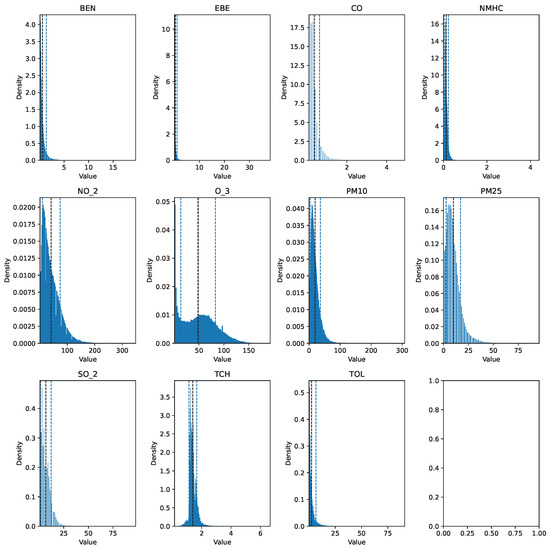
Figure 1.
Histogram of the raw pollutant data for 2017.
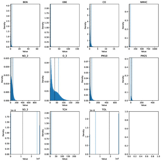
Figure 2.
Histogram of the raw pollutant data over the 18-year period.
The first step taken was the imputation of missing values using the interpolation method time to account for temporal patterns and to ensure consistency in the irregularly sampled data points. Prior to further modifications, the AQI category of each row was added to a new column AQI_Index, where the AQI corresponds to the “worst level” for any of the five pollutants, according to Table 1. An additional column, AQI_GenPop_Index, was introduced to represent the binary AQI values, indicating the air quality’s suitability for the general population. Subsequently, outliers from the pollutant columns were removed using the interquartile range (IQR), as the data exhibited high skewness. Finally, the pollutant columns were normalized using z-score normalization to have a mean of 0 and a standard deviation of 1. The clean features can be seen in Figure 3 and Figure 4. The target variable distribution is shown in Figure 5 and Figure 6.
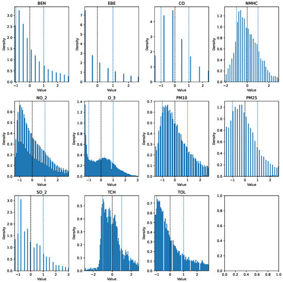
Figure 3.
Clean 2017 data (Training Set).
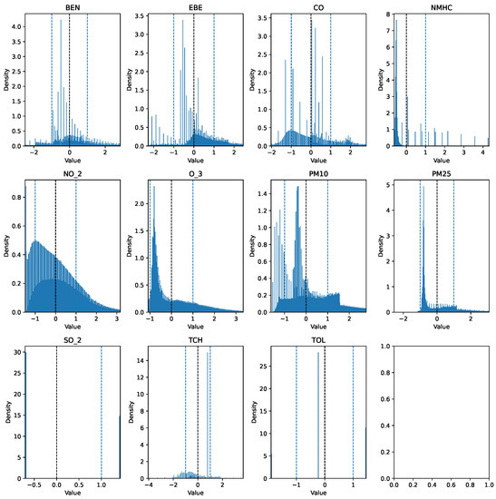
Figure 4.
Clean data over the 18-year period (testing set).
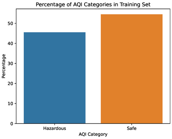
Figure 5.
Percentage of the AQI values in the training set.
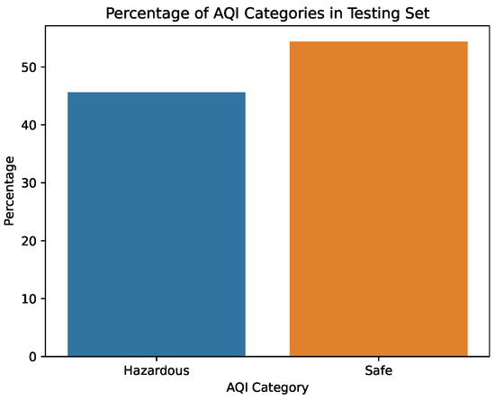
Figure 6.
Percentage of AQI values in the testing dataset.
4.2. Bayesian Logistic Regression
4.2.1. Model Definition
The training and evaluation data are imported and the relevant pollutant columns are selected as the features, while AQI_GenPop_Index is selected as the target column. This is followed by the design of the Bayesian Logistic Regression model using pymc3 for the prediction of the binary AQI categories. A pymc3 model object, called the AQI_model, is initialized and used to define priors that follow the normal distribution for both the coefficients(coeffs) and the model bias, while the coeffs are set to have an initial value of 0. The normal distribution is selected as we do not have any prior knowledge or preference for specific values of coeffs and bias [48].
Bayesian Logistic Regression is employed to estimate the probability of a binary variable (here, safe or hazardous) based on predictor variables (here: pollutants). The logistic function, also known as the sigmoid function, maps the linear combination of predictors and coefficients, along with a bias term, to a probability value between 0 and 1. In our implementation, we use the Theano library to efficiently compute the sigmoid function while ensuring numerical stability.
The probability of the positive class (1, representing “hazardous”) is calculated using the logistic function. This involves taking the inner product of the feature vector X_train and the coefficients, adding the bias term, and passing the result through the logistic function to obtain a probability value.
The resulting probability values, denoted as p, are utilized to model the observed binary variable y_train by employing the Bernoulli likelihood function. The model aims to estimate the probability of a sample belonging to the positive data class based on the input characteristics, as well as the probability of observing the actual binary response variable y_train. This concludes the model definition.
4.2.2. MCMC Sampling
After defining the model, posterior distribution sampling is performed using Markov Chain Monte Carlo (MCMC) techniques. Several algorithms are tested, with a particular preference for NUTS, and various tuning parameters are manually adjusted to optimize the prediction accuracy, as shown in Table 2 and Table 3. The target_accept argument determines the desired acceptance rate for the sampler, while the tune argument specifies the number of initial samples to be discarded before recording the results. The arguments chains and cores specify the numbers of parallel chains and cores used for sampling. Following sampling, a trace is generated for each model parameter using the pm.trace() function, which contains the posterior distribution samples of the coefficients and bias.
Table 2.
Classification metrics for various MCMC tuning parameters using five features.
Table 3.
Classification Metrics for various MCMC tuning parameters using 11 features.
4.2.3. Class Prediction on Unseen Data
Prediction for the Sensitivity Analysis
In the sensitivity analysis on the pandas data frame, predictions on unseen data are made using a predict_proba() function, as seen in Listing 1. This function calculates the predicted probabilities of the variable belonging to the positive class in a similar manner to the training model by taking the inner product of X_test and the posterior mean of the coefficients, along with the mean of the bias obtained from the MCMC trace. This result is passed to the logistic function, resulting in the predicted probability y_test_pred_proba. The predicted class y_test_pred is determined by selecting the class with the highest predicted probability, as shown in Listing 1.
| Listing 1: Predictions for Pandas Test Data. |
| def predi c t_proba (X, t r a c e ) : |
| l i n e a r = np . dot (X, t r a c e [ ‘ ‘ c o e f f s ’ ’ ] . mean ( a x i s = 0) ) |
| + t r a c e [ ‘ ‘ bi a s ’ ’ ] . mean ( ) |
| proba = 1 / (1 + np . exp(− l i n e a r ) ) |
| return np . column_stack ( ( 1 − proba , proba ) ) |
| y_test_pred_proba = predict_proba ( X_tes t , t r a c e ) |
| y_tes t_pred = np . argmax ( y_test_pred_proba , a x i s = 1) |
The evaluation metrics are computed using the scikit-learn.metrics library and can be seen in Table 2 and Table 3. These results are discussed in Section 5.1.
Predictions on the 18-Year Data in Apache Spark
We follow a similar approach as in the previous chapter, where we define the Bayesian Logistic Regression model. However, this time we train the model using the entire pandas data frame and make predictions on new and unknown data spanning eighteen years, utilizing the Apache Spark environment. The model definition and MCMC sampling procedures remain unchanged.
As for the predictions, instead of using np.column_stack, like in Listing 1, we combine the probabilities into a two-item array. To compute the linear combination of features and coefficients, we use the sum function instead of numpy’s dot function. While numpy’s dot function is typically used for matrix multiplication, the sum function simply adds the elements of a matrix. In the context of the Bayesian logistic regression, the linear combination of features and coefficients represents an inner product rather than a simple sum. However, given that we process one line at a time in Spark, the sum function suffices for calculating the linear combination. The above is achieved with the help of the user-defined function predict_proba_udf, as seen in Listing 2.
| Listing 2: User-defined predict_proba() function in pyspark. |
| @udf ( returnType=ArrayType (DoubleType ( ) ) ) |
| def predict_proba_udf ( c o e f f s _ l i s t , bias_value , * f e a tur e s ) : |
| l i n e a r = sum ( [ f e a tur e s [ i ] * c o e f f s _ l i s t [ i ] |
| for i in range ( len ( c o e f f s _ l i s t ) ) ] ) + bias_value |
| proba = 1 / (1 + math . exp(− l i n e a r ) ) |
| return [1 − proba , proba ] |
In the final definition of y_pred, we explore different decision threshold values to account for the roughly balanced nature of the classes that we aim to predict on the unknown data. It is important to note that y_test_pred_proba, mentioned in Listing 1, is a two-dimensional numpy array, where each row represents the predicted probabilities for each class.
By using np.argmax, we obtain the index of the highest probability along the second axis, which corresponds to the classes. Consequently, the predicted class y_test_pred can be either 0 or 1.
In Apache Spark, we directly calculate the probability of the positive class (col(“proba”)[1]) and then apply a threshold to determine the predicted label, shown in Listing 3. Although the notation might be different, the underlying concept remains the same, as both approaches involve computing the probability of the positive class and converting it into a binary label.
| Listing 3: Predicted probabilities and classes in pyspark. |
| spark_df = spark_df .withColumn ( ‘ ‘ proba ’ ’ , |
| predict_proba_udf ( coe f f s _ a r r ay , l i t ( bias_value ) , |
| * [ col ( c ) for c in feature_columns ] ) ) |
| spark_df=spark_df .withColumn ( ‘ ‘ y_pred ’ ’ , ( col ( ‘ ‘ proba ’ ’ ) [ 1 ] |
| >=threshold ) . c a s t (DoubleType ( ) ) ) |
The evaluation metrics for different thresholds can be seen in Table 4 and are discussed in Section 5.2.
Table 4.
Bayesian Logistic Regression Metrics in Spark for different decision threshold values.
5. Experimental Results
5.1. Sensitivity Analysis
The tuning parameters that were experimented with are as follows [49]:
- Tune: MCMC samplers rely on the concept of Markov chains, which converge to the stationary distribution of the defined model. To obtain unbiased samples, each chain should reach convergence. By setting the tuning parameter to a value (e.g., 1000), the chain iterates 1000 times to achieve convergence before sampling from the distribution begins. The default value is 1000.
- Draws: This parameter determines the number of samples to be taken from the model distribution after the tuning process. The default value is 1000.
- Chains: It is recommended that multiple chains (2–4) are run for reliable convergence diagnostics [49]. The number of chains is set to two by default or is equal to the number of available processors.
Table 2 and Table 3 present the model evaluation metrics obtained by varying the tuning parameters during MCMC sampling and using different numbers of features. The sensitivity analysis is initially performed on a set of five features, NO, O, PM, PM, and SO (which are used in the AQI calculation. Next, we incorporate BEN, EBE, CO, NMHC, TCH, and TOL into the model features, encompassing all pollutants in the dataset, resulting in a total of 11 features. By adjusting these tuning parameters and exploring different combinations of features, we obtain a comprehensive evaluation of the model’s performance.
Several observations can be made regarding the sampling process, model performance, the impact of tuning parameters, and the number of features. Our key findings include:
- Sampling Efficiency: Smaller draws and a tuning value of around 75–100% of the number of samples result in improved sampling and successful predictions on unknown data. Increasing the number of samples beyond a certain point does not provide additional information about the posterior distribution of the model.
- Model Complexity and Feature Set: Models with a smaller feature set tend to perform better than those with a larger set of 11 features. This is expected because sampling from high-dimensional distributions (such as those with more features) implies a higher model complexity and can lead to decreased performance.
- Convergence of the Sampling Algorithm: The sampling algorithm demonstrates convergence for different tuning parameters, as seen in Figure 7, but this does not guarantee successful predictions on unknown data. Convergence refers to the algorithm’s stability and not necessarily to the accuracy of predictions.
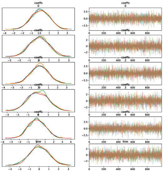 Figure 7. MCMC trace KDE and samples for five features.
Based on these observations, the following conclusions can be drawn:
- Draw: The number of samples required for MCMC sampling depends on the complexity of the posterior distribution being sampled rather than the number of features. Increasing the number of features generally increases the complexity, requiring more samples for accurate estimation.
- Tune: Larger "tune" values can prolong the adjustment phase, slowing down sampling and potentially leading to overfitting. Higher tune values may also result in samples with high autocorrelation, hindering accurate estimation. Conversely, a lower tune value leads to a shorter fitting phase, incomplete sampling, and biased estimation of the posterior distribution. Here, we check the model bias by comparing the mean of the target and predicted labels, as seen in Table 5.
Table 5. Model bias check: If the average value of the target column is similar to the average value of the predicted labels, the model is unbiased.
- Number of Features: The number of features in a model does not necessarily translate to more reliable beliefs. The reliability of beliefs depends on the data themselves and the estimates of the model parameters. While adding more features can increase the available information, it also increases the risk of overfitting. On the contrary, using fewer features may lead to underfitting, where the model is too simplistic and fails to capture the data complexity.
In summary, the optimal tuning parameters and a number of features should be carefully chosen to balance the model complexity, convergence, and prediction accuracy. Here, we conclude that the best choice for our model is draw = 1000, tune = 800–1000, and chains = 4 for the five-pollutant feature set.
5.2. Predictions in Apache Spark for Different Decision Thresholds
Having evaluated the model’s accuracy on small training and testing datasets, we now proceed to the retraining of the model on the 2017 pandas data frame. The goal is to make predictions on 18 years of unseen data using Pyspark for scalable big data management.
The evaluation metrics seen in Table 4 represent the performance of the classifier on the unknown data. During our experiment, we explored various decision threshold values for proba[1], as seen in Listing 3. This threshold determines the minimum probability at which the model classifies a case as positive.
For the evaluation, we use the following metrics: true positive (TP), true negative (TN), false positive (FP), and false negative (FN). It is worth noting that MCMC sampling is carried out using the following parameters: draw = 1000, tune = 1000, chains = 4, init=’advi’, n_init = 50,000, and the five feature set.
We observe that higher values of the threshold lead to a more conservative model that makes fewer false positive predictions but more false negatives (Table 4). At the lowest threshold, the model exhibits low precision, with a value of 0.4584, indicating a significant number of incidents being incorrectly classified as false positives (hazardous). As the threshold increases, both the accuracy and precision of the model improve. The maximum values of 0.8791 and 0.9932, respectively, are achieved for a decision threshold of 0.505. However, beyond this threshold, the model’s accuracy begins to decline again. These findings clearly demonstrate the substantial influence of the decision threshold on the classification model’s performance. Ultimately, the selection of an appropriate threshold depends on the specific requirements of each problem, such as the relative costs associated with false positives and false negatives [50].
Here, the objective is to classify the AQI as either “safe” (negative) or “hazardous” (positive) for the general population. This means that it is crucial to minimize false negatives, as misclassifying the air quality as “safe” could unknowingly subject the general population to harmful air pollution. Hence, our primary concern lies in the metric of recall/specificity, which quantifies the model’s ability to correctly identify safe air quality instances (or true negatives, TN).
Upon analyzing the results, we find that, for a decision threshold of 0.505, the recall/specificity metric reaches a value of 0.9958. This indicates that the model consistently and accurately predicts the safe air quality, as evidenced by the high number of true negatives (TN). For this reason, we consider the threshold of 0.505 to be the optimal choice. This decision is based not only on the superior overall model performance achieved at this threshold but also on the fact that selecting higher thresholds would lead to an increase in false negative predictions, which is undesirable in our context.
Hence, we conclude that the threshold of 0.505 offers the best balance in terms of the overall model performance, recall/specificity, and the prevention of false negative predictions.
5.3. Bayesian vs. Frequentist Logistic Regression in Apache Spark
This research concludes with the examination, training, and testing of a Frequentist Logistic Regression model using the predefined algorithms in Pyspark’s MLlib library. The evaluation metrics of both models, trained and assessed on identical training and control sets, are presented in Table 6, using a consistent decision threshold of 0.505.
Table 6.
Frequentist and Bayesian Logistic Regression evaluation metrics in Spark with five features and a decision threshold equal to 0.505.
By comparing the two models, we observe that they demonstrate similar levels of accuracy and duration for the training and testing processes. The precision and ROC AUC metrics differ significantly for the two models, with the Bayesian model performing better in terms of precision and the Frequentist model having a higher ROC score, indicating its overall superior performance in terms of balancing the true positive rate against the false positive rate. The confusion matrices for each model for various thresholds are shown in Figure 8, Figure 9 and Figure 10 while the ROC curve, as well as the AUC score for each method, are shown in Figure 11.
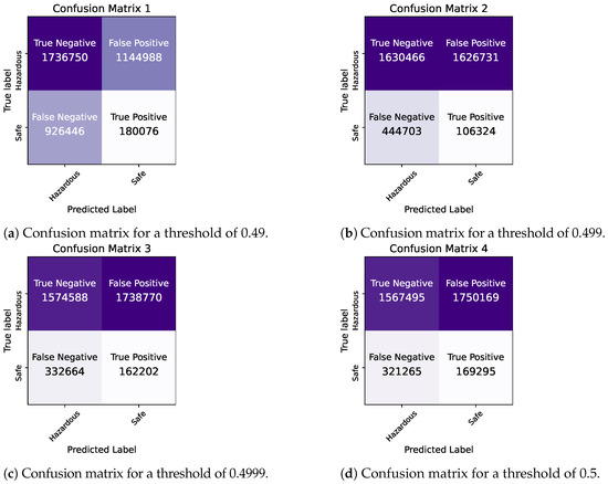
Figure 8.
Bayesian Logistic Regression in Pyspark: Confusion matrices for thresholds of 0.49–0.5.
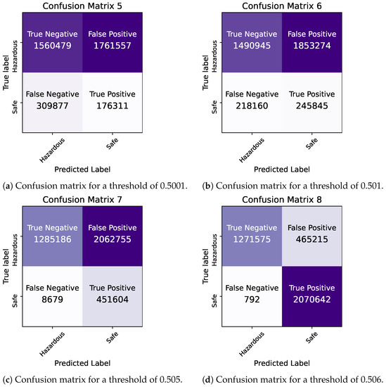
Figure 9.
Bayesian Logistic Regression in Pyspark: confusion matrices for thresholds of 0.5001–0.506.
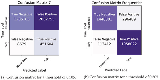
Figure 10.
Bayesian vs. Frequentist Logistic Regression in Pyspark: confusion matrices for a threshold of 0.505.
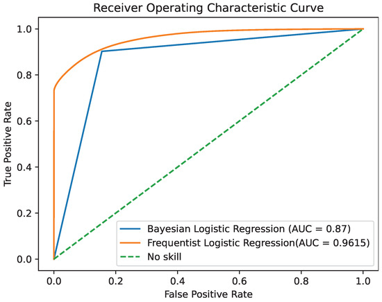
Figure 11.
ROC area under the curve for the two models.
Given the significance of true negatives in this specific problem, the recall/specificity metric is assumed to be of utmost importance. Notably, in Table 6, the Bayesian model demonstrates a superior performance compared to its Frequentist counterpart when considering this specific metric, highlighting its effectiveness in accurately identifying true negatives. This is crucial for ensuring that the Air Quality Index (AQI) category is not mistakenly classified as “safe”, thereby preventing inadvertent exposure of the general population to harmful air. The examination of the confusion matrices supports the idea that the Bayesian model exhibits a greater number of true negatives compared to the Frequentist model, a crucial aspect for addressing the problem at hand.
As a final conclusion, the Bayesian model provides more up-to-date estimates by incorporating uncertainty, instilling a higher level of confidence in the data quality. Consequently, based on these observations, it is safe to say that Bayesian Logistic Regression is the best option between the two for this specific case.
6. Conclusions and Future Work
6.1. Conclusions
In this study, we introduced and presented the first-ever Markov Chain Monte Carlo (MCMC) classifier in the context of environmental data analysis. Our focus on model simplicity revealed that an equilibrium between the number of features and model complexity is crucial for preventing overfitting and optimizing the predictive accuracy. Specifically, our MCMC classifier achieved an outstanding accuracy of 87.91% and a remarkable recall/specificity of 99.58% at a decision threshold of 0.505, demonstrating its efficacy in air quality prediction.
Furthermore, we underpinned the essentiality of custom decision thresholds and the careful selection of problem-specific evaluation metrics. This approach focuses on addressing the consequences of false negative predictions and optimizing the trade-offs between false positives and negatives. Moreover, our research demonstrates the superior capabilities of Bayesian machine learning models over their Frequentist counterparts in managing the inherent uncertainties of environmental datasets. Simultaneously, this work underscores the notable role of Apache Spark in big data management. Its distributed computing capabilities facilitate the handling of large environmental datasets, ultimately enhancing the model’s performance, reliability, and scalability. The scalability of Apache Spark is particularly valuable in the spectrum of environmental data analysis, where the volume and complexity of data pose significant challenges. Through the utilization of Apache Spark, this study explored the scalability of our MCMC-based classifier, enabling comprehensive insights and accurate predictions on larger datasets. This not only enhanced the model performance but also facilitated the exploration of complex environmental problems, generating more reliable and robust results. The findings presented in Section 5.2 highlight the potential of Apache Spark for use in environmental data analysis as it overcomes the challenges faced while working with such data, while also incorporating prior knowledge, leading to evidence-based decisions.
Regarding future work, several potential extensions can be considered. These include the development of a multiclass Bayesian classification model to predict all categories of the Air Quality Index (AQI), refining prior distributions to enhance the sampling and estimation efficiency, exploring Bayesian models’ application to alternative environmental datasets, such as recyclables management, and integrating Pymc with Pyspark for distributed Bayesian modeling. These directions aim to expand the capabilities of our classifier for environmental data analysis, fostering a deeper understanding of air quality data and supporting informed decision-making in environmental management and public health. As future directions, we will focus on developing a multiclass Bayesian classification model, refining prior distributions, and broadening Bayesian models’ applications to more complex environmental datasets. These improvements aim to further exploit the potential of our pioneering MCMC classifier, deepen our understanding of air quality data, and support informed decision-making processes in environmental management and public health.
6.2. Future Work
6.2.1. Environmental Data Analysis Applications
Future work on environmental data analysis must address various challenges such as handling large volumes of data, managing uncertainties in characteristics and predictions, minimizing computational complexities, and exploring intricate data relationships [51,52]. Novel techniques to be pursued include stochastic process modeling for environmental systems [53,54], statistical computation methods for detecting patterns and trends [55,56], and deep learning approaches to uncover hidden correlations [57,58,59,60]. The application of intelligent gas detection systems, IoT, and advanced sensor technologies for real-time monitoring can further enhance this field [61,62,63]. Notably, the integration of AutoML with Bayesian optimizations, as presented in [64], offers promising results.
Moreover, the application of TinyML, which is characterized by lightweight machine learning models optimized for resource-constrained peripheral devices, represents a new frontier in environmental monitoring, according to [65]. Expanding the scope of TinyML applications and integrating them with environmental sensors and networks could pave the way for economically viable real-time data analysis solutions. In addition, the research and development of novel clustering methods, such as those suggested in [66], could potentially be beneficial. These techniques can aid in the unraveling of complex environmental patterns, thereby enhancing the precision and robustness of machine learning models within complex and high-dimensional datasets.
The scope and variety of possible future research in environmental data analysis is vast and requires significant progress to be made in the fields of data science, modeling, and distributed and cloud computing. Such research should focus on managing the complexities of large-scale data analysis and the inherent uncertainty in environmental data. Interdisciplinary collaborations and novel research practices are essential to address the multifaceted challenges in earth and environmental sciences. Pursuing these areas will underpin effective environmental issue management and promote informed, sustainable decision-making.
6.2.2. Bayesian Machine Learning and Bayesian Inference
Future research in Bayesian machine learning should focus on improving model accuracy and scalability, particularly within the context of Markov Chain Monte Carlo (MCMC) applications in Apache Spark environments. Emphasis should be placed on the development of efficient methods for the post hoc computation of high-dimensional targets, investigating the potential of normalized flows for adaptive MCMC and creating Bayesian coresets for data compression before sampling to mitigate the computational burden [51].
There is a significant need to explore distributed Bayesian inference for dependent, high-dimensional models, moving beyond the current focus on independent data models [67]. Methods that capitalize on the low-dimensional structures of high-dimensional problems can be valuable, along with those that reduce bias and variance, promote asynchronous updates, and facilitate automated diagnosis.
Furthermore, to address larger and more complex problems, the scalability of Bayesian models should be enhanced using distributed memory technologies. Optimization strategies for these technologies can help to achieve faster and more energy-efficient predictions [68]. This necessitates the development of novel algorithms and techniques for Bayesian inference suitable for distributed memory architectures. Investigation into alternative formulations of the Bayesian theorem for distributed memory and hybrid architectures that combine Bayesian models with other machine learning methods, such as neural networks and decision trees, could also be of significant value.
Ultimately, the future of Bayesian machine learning involves its successful integration into existing machine learning technologies, focusing on speed, computational complexity, energy efficiency, and cost-effectiveness. This exploration will unlock the full potential of Bayesian models in addressing real-world challenges, promoting advancements in data analysis and decision-making.
Author Contributions
E.V., C.K., A.K., D.T. and S.S. conceived the idea, designed and performed the experiments, analyzed the results, drafted the initial manuscript and revised the final manuscript. All authors have read and agreed to the published version of the manuscript.
Funding
This research received no external funding.
Data Availability Statement
The data presented in this study are available on request from the corresponding author.
Conflicts of Interest
The authors declare no conflict of interest.
Abbreviations
The following abbreviations are used in this manuscript:
| API | Application Programming Interface |
| AQI | Air Quality Index |
| AUC | Area Under the Curve |
| FN | False Negative |
| FP | False Positive |
| HMC | Hamiltonian Monte Carlo |
| IQR | Interquartile Range |
| MCMC | Markov Chain Monte Carlo |
| MH | Metropolis-Hastings |
| ML | Machine Learning |
| NUTS | No-U-Turn Sampler |
| RDD | Resilient Distributed Dataset |
| ROC | Receiver Operating Characteristic |
| TN | True Negative |
| TP | True Positive |
| UDF | User-Defined Function |
| IoT | Internet of Things |
| EI | Environment Information |
| IT | Information Technology |
References
- Villanueva, F.; Ródenas, M.; Ruus, A.; Saffell, J.; Gabriel, M.F. Sampling and analysis techniques for inorganic air pollutants in indoor air. Appl. Spectrosc. Rev. 2021, 57, 531–579. [Google Scholar] [CrossRef]
- Martínez Torres, J.; Pastor Pérez, J.; Sancho Val, J.; McNabola, A.; Martínez Comesaña, M.; Gallagher, J. A Functional Data Analysis Approach for the Detection of Air Pollution Episodes and Outliers: A Case Study in Dublin, Ireland. Mathematics 2020, 8, 225. [Google Scholar] [CrossRef]
- Karras, C.; Karras, A.; Avlonitis, M.; Giannoukou, I.; Sioutas, S. Maximum Likelihood Estimators on MCMC Sampling Algorithms for Decision Making. In Proceedings of the Artificial Intelligence Applications and Innovations, AIAI 2022 IFIP WG 12.5 International Workshops, Creta, Greece, 17–20 June 2022; Maglogiannis, I., Iliadis, L., Macintyre, J., Cortez, P., Eds.; Springer International Publishing: Cham, Switzerland, 2022; pp. 345–356. [Google Scholar]
- Wang, G.; Wang, T. Unbiased Multilevel Monte Carlo methods for intractable distributions: MLMC meets MCMC. arXiv 2022, arXiv:2204.04808. [Google Scholar]
- Braham, H.; Berdjoudj, L.; Boualem, M.; Rahmania, N. Analysis of a non-Markovian queueing model: Bayesian statistics and MCMC methods. Monte Carlo Methods Appl. 2019, 25, 147–154. [Google Scholar] [CrossRef]
- Altschuler, J.M.; Talwar, K. Resolving the Mixing Time of the Langevin Algorithm to its Stationary Distribution for Log-Concave Sampling. arXiv 2022, arXiv:2210.08448. [Google Scholar]
- Paguyo, J. Mixing times of a Burnside process Markov chain on set partitions. arXiv 2022, arXiv:2207.14269. [Google Scholar]
- Dymetman, M.; Bouchard, G.; Carter, S. The OS* algorithm: A joint approach to exact optimization and sampling. arXiv 2012, arXiv:1207.0742. [Google Scholar]
- Jaini, P.; Nielsen, D.; Welling, M. Sampling in combinatorial spaces with survae flow augmented mcmc. In Proceedings of the International Conference on Artificial Intelligence and Statistics, PMLR, Virtual, 13–15 April 2021; pp. 3349–3357. [Google Scholar]
- Vono, M.; Paulin, D.; Doucet, A. Efficient MCMC sampling with dimension-free convergence rate using ADMM-type splitting. J. Mach. Learn. Res. 2022, 23, 1100–1168. [Google Scholar]
- Pinski, F.J. A Novel Hybrid Monte Carlo Algorithm for Sampling Path Space. Entropy 2021, 23, 499. [Google Scholar] [CrossRef]
- Beraha, M.; Argiento, R.; Møller, J.; Guglielmi, A. MCMC Computations for Bayesian Mixture Models Using Repulsive Point Processes. J. Comput. Graph. Stat. 2022, 31, 422–435. [Google Scholar] [CrossRef]
- Cotter, S.L.; Roberts, G.O.; Stuart, A.M.; White, D. MCMC Methods for Functions: Modifying Old Algorithms to Make Them Faster. Stat. Sci. 2013, 28, 424–446. [Google Scholar] [CrossRef]
- Craiu, R.V.; Levi, E. Approximate Methods for Bayesian Computation. Annu. Rev. Stat. Its Appl. 2023, 10, 379–399. [Google Scholar] [CrossRef]
- Van Ravenzwaaij, D.; Cassey, P.; Brown, S.D. A simple introduction to Markov Chain Monte–Carlo sampling. Psychon. Bull. Rev. 2018, 25, 143–154. [Google Scholar] [CrossRef] [PubMed]
- Karras, C.; Karras, A.; Avlonitis, M.; Sioutas, S. An Overview of MCMC Methods: From Theory to Applications. In Proceedings of the Artificial Intelligence Applications and Innovations, AIAI 2022 IFIP WG 12.5 International Workshops, Creta, Greece, 17–20 June 2022; Maglogiannis, I., Iliadis, L., Macintyre, J., Cortez, P., Eds.; Springer International Publishing: Cham, Switzerland, 2022; pp. 319–332. [Google Scholar]
- Snoek, J.; Larochelle, H.; Adams, R.P. Practical bayesian optimization of machine learning algorithms. Adv. Neural Inf. Process. Syst. 2012, 25. [Google Scholar]
- Theodoridis, S. Machine Learning: A Bayesian and Optimization Perspective; Academic Press: Cambridge, MA, USA, 2015. [Google Scholar]
- Elgeldawi, E.; Sayed, A.; Galal, A.R.; Zaki, A.M. Hyperparameter Tuning for Machine Learning Algorithms Used for Arabic Sentiment Analysis. Informatics 2021, 8, 79. [Google Scholar] [CrossRef]
- Band, S.S.; Janizadeh, S.; Saha, S.; Mukherjee, K.; Bozchaloei, S.K.; Cerdà, A.; Shokri, M.; Mosavi, A. Evaluating the Efficiency of Different Regression, Decision Tree, and Bayesian Machine Learning Algorithms in Spatial Piping Erosion Susceptibility Using ALOS/PALSAR Data. Land 2020, 9, 346. [Google Scholar] [CrossRef]
- Itoo, F.; Singh, S. Comparison and analysis of logistic regression, Naïve Bayes and KNN machine learning algorithms for credit card fraud detection. Int. J. Inf. Technol. 2021, 13, 1503–1511. [Google Scholar] [CrossRef]
- Wu, J.; Chen, X.Y.; Zhang, H.; Xiong, L.D.; Lei, H.; Deng, S.H. Hyperparameter optimization for machine learning models based on Bayesian optimization. J. Electron. Sci. Technol. 2019, 17, 26–40. [Google Scholar]
- Wei, X.; Wang, H. Stochastic stratigraphic modeling using Bayesian machine learning. Eng. Geol. 2022, 307, 106789. [Google Scholar] [CrossRef]
- Hitchcock, D.B. A history of the Metropolis–Hastings algorithm. Am. Stat. 2003, 57, 254–257. [Google Scholar] [CrossRef]
- Robert, C.; Casella, G.; Robert, C.P.; Casella, G. Metropolis–hastings algorithms. In Introducing Monte Carlo Methods with R; Springer: Berlin/Heidelberg, Germany, 2010; pp. 167–197. [Google Scholar]
- Hassibi, B.; Hansen, M.; Dimakis, A.G.; Alshamary, H.A.J.; Xu, W. Optimized Markov Chain Monte Carlo for Signal Detection in MIMO Systems: An Analysis of the Stationary Distribution and Mixing Time. IEEE Trans. Signal Process. 2014, 62, 4436–4450. [Google Scholar] [CrossRef]
- Chib, S.; Greenberg, E. Understanding the metropolis-hastings algorithm. Am. Stat. 1995, 49, 327–335. [Google Scholar]
- Hoogerheide, L.F.; van Dijk, H.K.; van Oest, R.D. Simulation Based Bayesian Econometric Inference: Principles and Some Recent Computational Advances. Econom. J. 2007, 215–280. [Google Scholar] [CrossRef]
- Johannes, M.; Polson, N. MCMC methods for continuous-time financial econometrics. In Handbook of Financial Econometrics: Applications; Elsevier: Amsterdam, The Netherlands, 2010; pp. 1–72. [Google Scholar]
- Flury, T.; Shephard, N. Bayesian inference based only on simulated likelihood: Particle filter analysis of dynamic economic models. Econom. Theory 2011, 27, 933–956. [Google Scholar] [CrossRef]
- Zuev, K.M.; Katafygiotis, L.S. Modified Metropolis–Hastings algorithm with delayed rejection. Probabilistic Eng. Mech. 2011, 26, 405–412. [Google Scholar] [CrossRef]
- Alotaibi, R.; Nassar, M.; Elshahhat, A. Computational Analysis of XLindley Parameters Using Adaptive Type-II Progressive Hybrid Censoring with Applications in Chemical Engineering. Mathematics 2022, 10, 3355. [Google Scholar] [CrossRef]
- Afify, A.Z.; Gemeay, A.M.; Alfaer, N.M.; Cordeiro, G.M.; Hafez, E.H. Power-modified kies-exponential distribution: Properties, classical and bayesian inference with an application to engineering data. Entropy 2022, 24, 883. [Google Scholar] [CrossRef] [PubMed]
- Elshahhat, A.; Elemary, B.R. Analysis for Xgamma parameters of life under Type-II adaptive progressively hybrid censoring with applications in engineering and chemistry. Symmetry 2021, 13, 2112. [Google Scholar] [CrossRef]
- Delmas, J.F.; Jourdain, B. Does waste-recycling really improve Metropolis-Hastings Monte Carlo algorithm? arXiv 2006, arXiv:math/0611949. [Google Scholar]
- Datta, S.; Gayraud, G.; Leclerc, E.; Bois, F.Y. Graph sampler: A C language software for fully Bayesian analyses of Bayesian networks. arXiv 2015, arXiv:1505.07228. [Google Scholar]
- Gamerman, D. Markov chain Monte Carlo for dynamic generalised linear models. Biometrika 1998, 85, 215–227. [Google Scholar] [CrossRef]
- Alvin J., K.C.; Vallisneri, M. Learning Bayes’ theorem with a neural network for gravitational-wave inference. arXiv 2019, arXiv:1909.05966. [Google Scholar]
- Vuckovic, J. Nonlinear MCMC for Bayesian Machine Learning. In Proceedings of the Neural Information Processing Systems, New Orleans, LA, USA, 28 November–9 December 2022. [Google Scholar]
- Green, S.R.; Gair, J. Complete parameter inference for GW150914 using deep learning. Mach. Learn. Sci. Technol. 2021, 2, 03LT01. [Google Scholar] [CrossRef]
- Martino, L.; Elvira, V. Metropolis sampling. arXiv 2017, arXiv:1704.04629. [Google Scholar]
- Catanach, T.A.; Vo, H.D.; Munsky, B. Bayesian inference of stochastic reaction networks using multifidelity sequential tempered Markov chain Monte Carlo. Int. J. Uncertain. Quantif. 2020, 10, 515–542. [Google Scholar] [CrossRef]
- Burke, N. Metropolis, Metropolis-Hastings and Gibbs Sampling Algorithms; Lakehead University Thunder Bay: Thunder Bay, ON, Canada, 2018. [Google Scholar]
- Apers, S.; Gribling, S.; Szilágyi, D. Hamiltonian Monte Carlo for efficient Gaussian sampling: Long and random steps. arXiv 2022, arXiv:2209.12771. [Google Scholar]
- Hoffman, M.D.; Gelman, A. The No-U-Turn sampler: Adaptively setting path lengths in Hamiltonian Monte Carlo. J. Mach. Learn. Res. 2014, 15, 1593–1623. [Google Scholar]
- Soluciones, D. Air Quality in Madrid (2001–2018). In Kaggle: A Platform for Data Science; Kaggle: San Francisco, CA, USA, 2018. [Google Scholar]
- Aguilar, P.M.; Carrera, L.G.; Segura, C.C.; Sánchez, M.I.T.; Peña, M.F.V.; Hernán, G.B.; Rodríguez, I.E.; Zapata, R.M.R.; Lucas, E.Z.D.; Álvarez, P.D.A.; et al. Relationship between air pollution levels in Madrid and the natural history of idiopathic pulmonary fibrosis: Severity and mortality. J. Int. Med. Res. 2021, 49, 03000605211029058. [Google Scholar] [CrossRef]
- Salvatier, J.; Wiecki, T.V.; Fonnesbeck, C. Probabilistic programming in Python using PyMC3. Peerj Comput. Sci. 2016, 2, e55. [Google Scholar] [CrossRef]
- Salvatier, J.; Wiecki, T.V.; Fonnesbeck, C. Sampling, PyMC3 Documentation. Online Documentation. 2021. Available online: https://www.pymc.io/projects/docs/en/v3/pymc-examples/examples/getting_started.html (accessed on 1 May 2023).
- Hossin, M.; Sulaiman, M.N. A review on evaluation metrics for data classification evaluations. Int. J. Data Min. Knowl. Manag. Process. 2015, 5, 1. [Google Scholar]
- Blair, G.S.; Henrys, P.; Leeson, A.; Watkins, J.; Eastoe, E.; Jarvis, S.; Young, P.J. Data science of the natural environment: A research roadmap. Front. Environ. Sci. 2019, 7, 121. [Google Scholar] [CrossRef]
- Kozlova, M.; Yeomans, J.S. Sustainability Analysis and Environmental Decision-Making Using Simulation, Optimization, and Computational Analytics. Sustainability 2022, 14, 1655. [Google Scholar] [CrossRef]
- Bhuiyan, M.A.M.; Sahi, R.K.; Islam, M.R.; Mahmud, S. Machine Learning Techniques Applied to Predict Tropospheric Ozone in a Semi-Arid Climate Region. Mathematics 2021, 9, 2901. [Google Scholar] [CrossRef]
- Del Giudice, D.; Löwe, R.; Madsen, H.; Mikkelsen, P.S.; Rieckermann, J. Comparison of two stochastic techniques for reliable urban runoff prediction by modeling systematic errors. Water Resour. Res. 2015, 51, 5004–5022. [Google Scholar] [CrossRef]
- Cheng, T.; Wang, J.; Li, X. A Hybrid Framework for Space–Time Modeling of Environmental Data. Geogr. Anal. 2011, 43, 188–210. [Google Scholar] [CrossRef]
- Chen, L.; He, Q.; Wan, H.; He, S.; Deng, M. Statistical computation methods for microbiome compositional data network inference. arXiv 2021, arXiv:2109.01993. [Google Scholar]
- Li, J.B.; Qu, S.; Metze, F.; Huang, P.Y. AudioTagging Done Right: 2nd comparison of deep learning methods for environmental sound classification. arXiv 2022, arXiv:2203.13448. [Google Scholar]
- Jubair, S.; Domaratzki, M. Crop genomic selection with deep learning and environmental data: A survey. Front. Artif. Intell. 2022, 5, 1040295. [Google Scholar] [CrossRef]
- Hsiao, H.C.W.; Chen, S.H.F.; Tsai, J.J.P. Deep Learning for Risk Analysis of Specific Cardiovascular Diseases Using Environmental Data and Outpatient Records. In Proceedings of the 2016 IEEE 16th International Conference on Bioinformatics and Bioengineering (BIBE), Taichung, Taiwan, 31 October–2 November 2016; pp. 369–372. [Google Scholar] [CrossRef]
- Jin, X.B.; Zheng, W.Z.; Kong, J.L.; Wang, X.Y.; Zuo, M.; Zhang, Q.C.; Lin, S. Deep-Learning Temporal Predictor via Bidirectional Self-Attentive Encoder–Decoder Framework for IOT-Based Environmental Sensing in Intelligent Greenhouse. Agriculture 2021, 11, 802. [Google Scholar] [CrossRef]
- Senthil, G.; Suganthi, P.; Prabha, R.; Madhumathi, M.; Prabhu, S.; Sridevi, S. An Enhanced Smart Intelligent Detecting and Alerting System for Industrial Gas Leakage using IoT in Sensor Network. In Proceedings of the 2023 5th International Conference on Smart Systems and Inventive Technology (ICSSIT), Tirunelveli, India, 23–25 January 2023; pp. 397–401. [Google Scholar] [CrossRef]
- Liu, B.; Zhou, Y.; Fu, H.; Fu, P.; Feng, L. Lightweight Self-Detection and Self-Calibration Strategy for MEMS Gas Sensor Arrays. Sensors 2022, 22, 4315. [Google Scholar] [CrossRef]
- Fascista, A. Toward Integrated Large-Scale Environmental Monitoring Using WSN/UAV/Crowdsensing: A Review of Applications, Signal Processing, and Future Perspectives. Sensors 2022, 22, 1824. [Google Scholar] [CrossRef] [PubMed]
- Karras, A.; Karras, C.; Schizas, N.; Avlonitis, M.; Sioutas, S. AutoML with Bayesian Optimizations for Big Data Management. Information 2023, 14, 223. [Google Scholar] [CrossRef]
- Schizas, N.; Karras, A.; Karras, C.; Sioutas, S. TinyML for Ultra-Low Power AI and Large Scale IoT Deployments: A Systematic Review. Future Internet 2022, 14, 363. [Google Scholar] [CrossRef]
- Karras, C.; Karras, A.; Giotopoulos, K.C.; Avlonitis, M.; Sioutas, S. Consensus Big Data Clustering for Bayesian Mixture Models. Algorithms 2023, 16, 245. [Google Scholar] [CrossRef]
- Krafft, P.M.; Zheng, J.; Pan, W.; Della Penna, N.; Altshuler, Y.; Shmueli, E.; Tenenbaum, J.B.; Pentland, A. Human collective intelligence as distributed Bayesian inference. arXiv 2016, arXiv:1608.01987. [Google Scholar]
- Winter, S.; Campbell, T.; Lin, L.; Srivastava, S.; Dunson, D.B. Machine Learning and the Future of Bayesian Computation. arXiv 2023, arXiv:2304.11251. [Google Scholar]


Disclaimer/Publisher’s Note: The statements, opinions and data contained in all publications are solely those of the individual author(s) and contributor(s) and not of MDPI and/or the editor(s). MDPI and/or the editor(s) disclaim responsibility for any injury to people or property resulting from any ideas, methods, instructions or products referred to in the content. |
© 2023 by the authors. Licensee MDPI, Basel, Switzerland. This article is an open access article distributed under the terms and conditions of the Creative Commons Attribution (CC BY) license (https://creativecommons.org/licenses/by/4.0/).