

Local Community Detection in Graph Streams with Anchors


Abstract
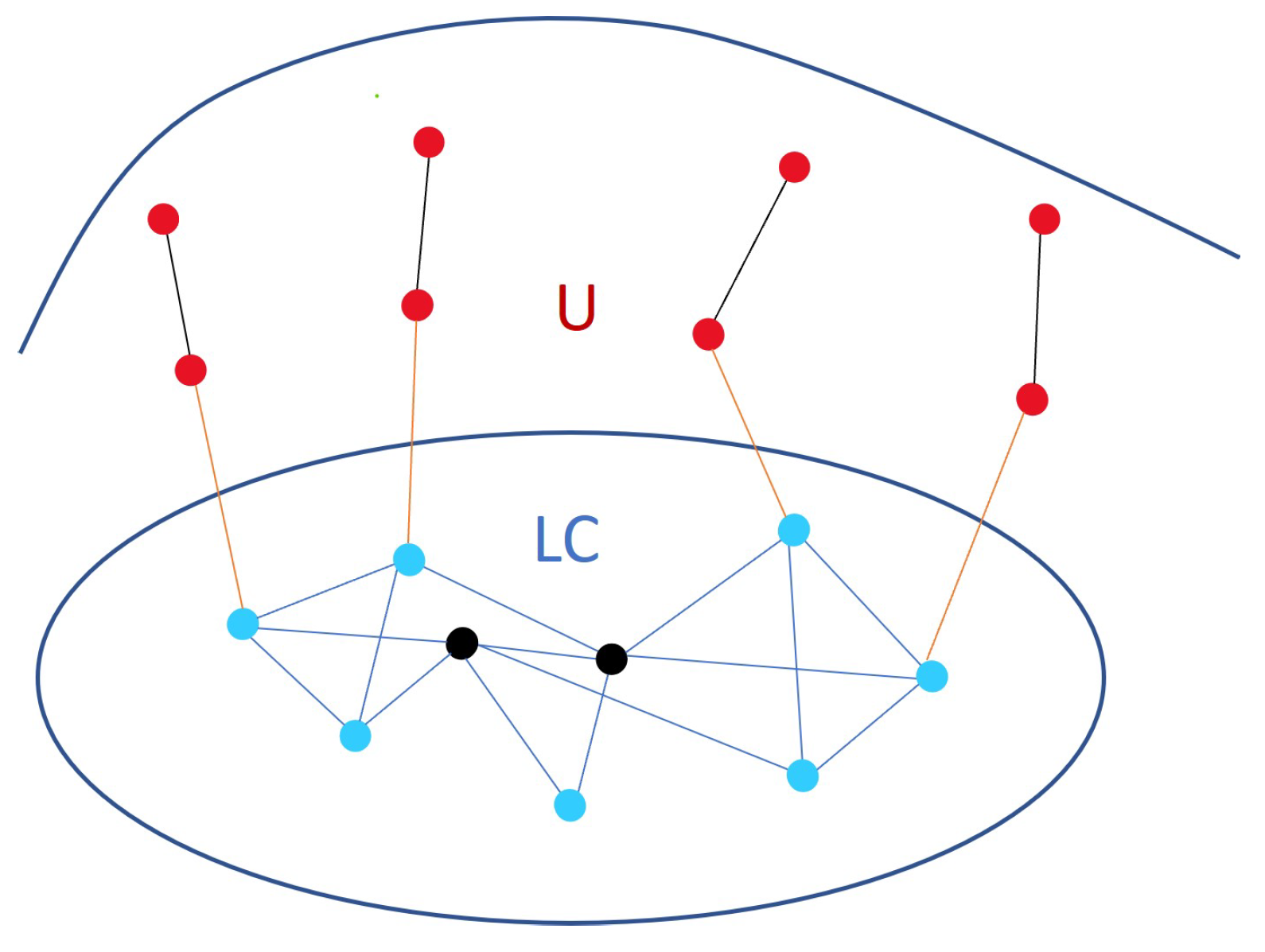
1. Introduction
Contributions
- From a modeling perspective, our contribution lies in introducing the notion of the anchor node in the local community detection problem into time-evolving networks.
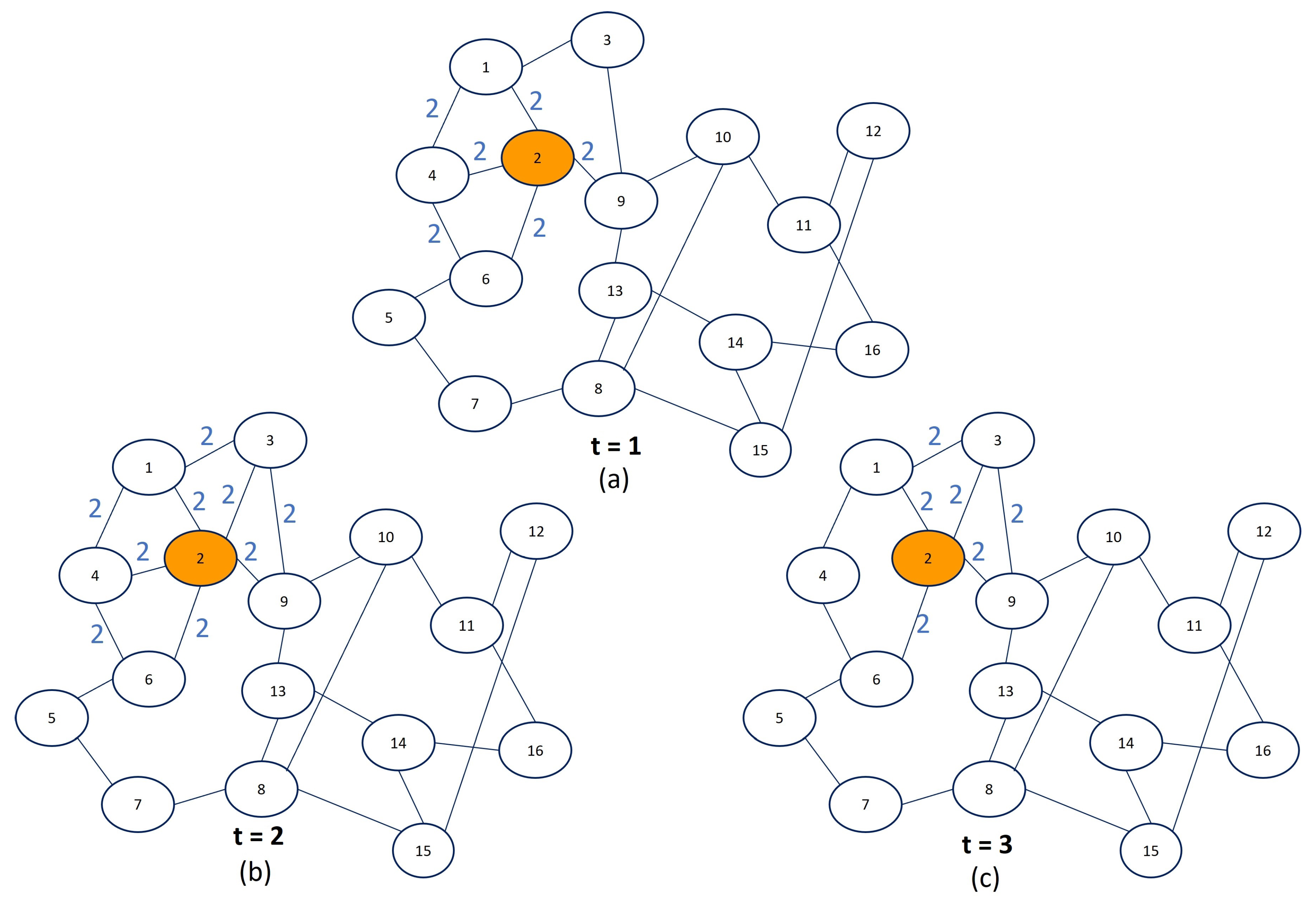
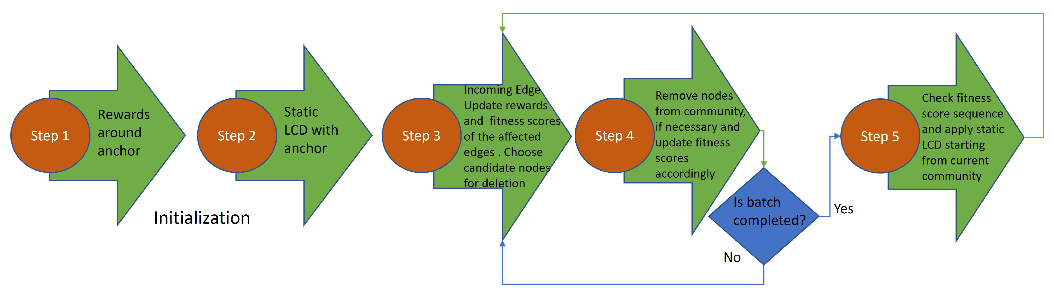
- From an algorithmic perspective, a general multi-step framework was proposed that can be used to detect stable communities of an important node in time-evolving networks.
2. Related Work
3. Problem Formulation and Methodology
3.1. Preliminaries
3.2. Problem Formulation
| Algorithm 1 Static algorithm [22] |
Input:
|
3.3. Local Community Detection in Graph Streams with Anchors
| Algorithm 2 The pseudo-code of the proposed LCDS-A framework |
Input:
|
Time Complexity
4. Experiments
4.1. Experiment Design
4.2. Datasets
4.2.1. Synthetic Datasets
4.2.2. Real Datasets
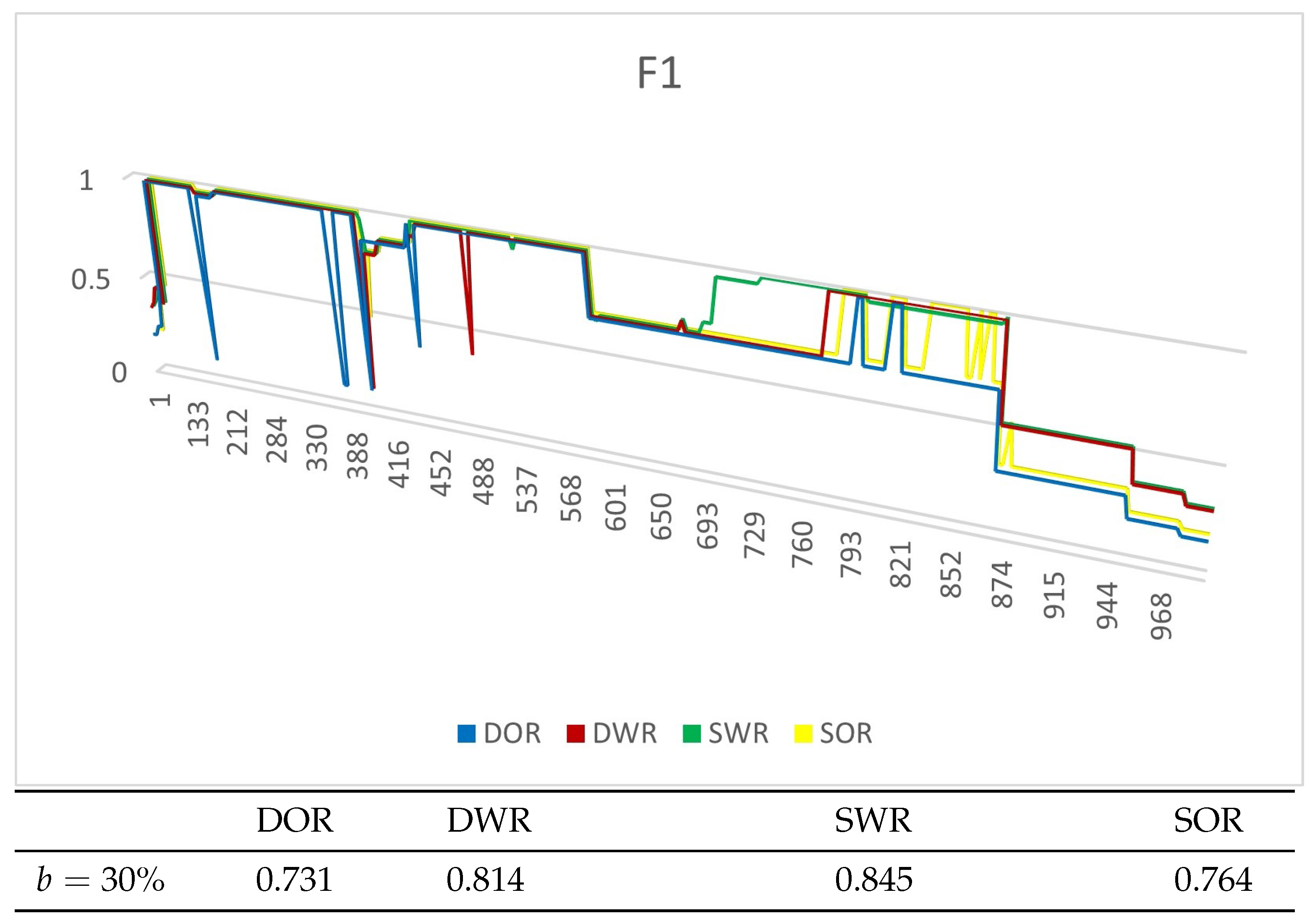
4.3. Evaluation Metrics
4.4. Experiment Results
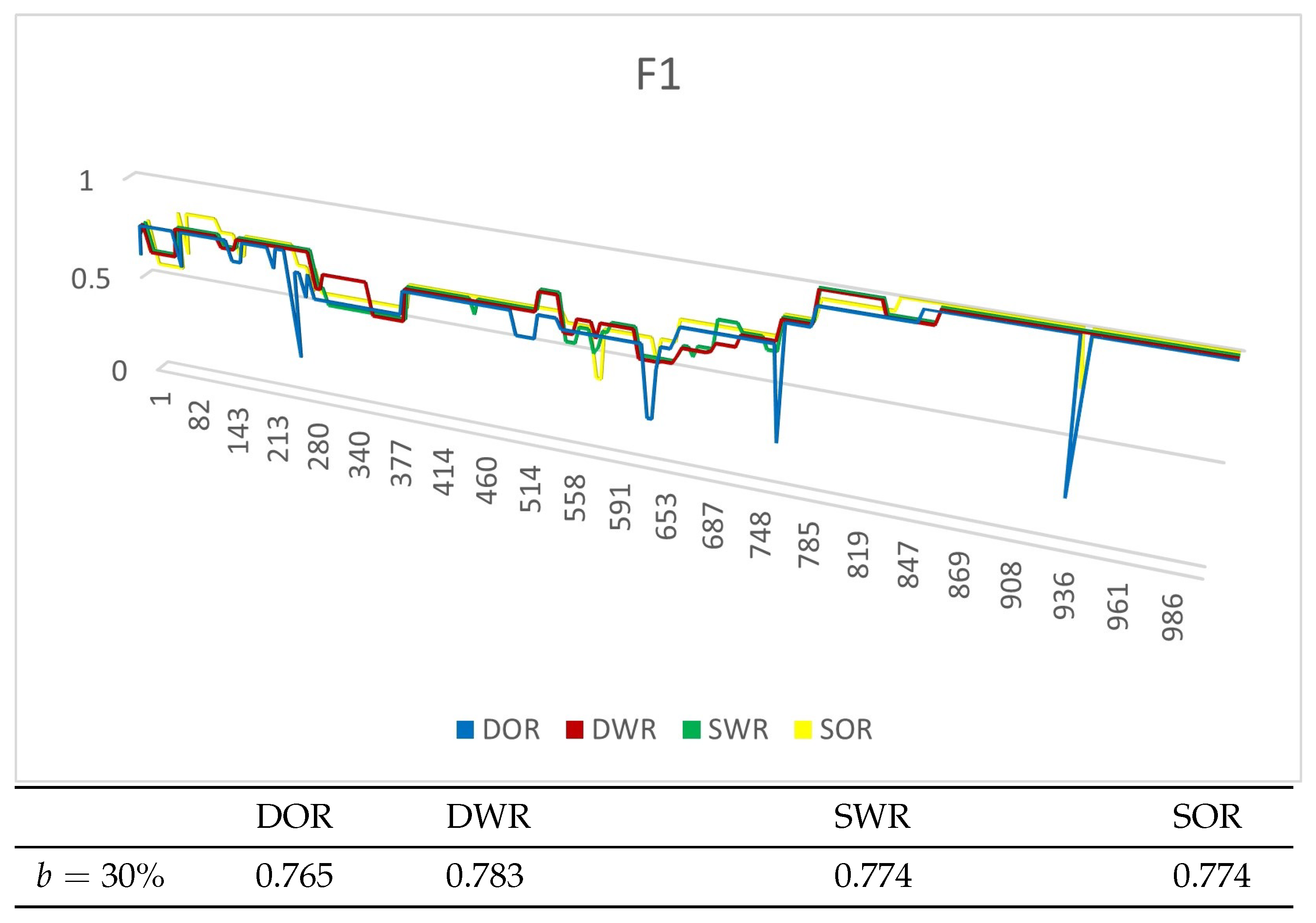
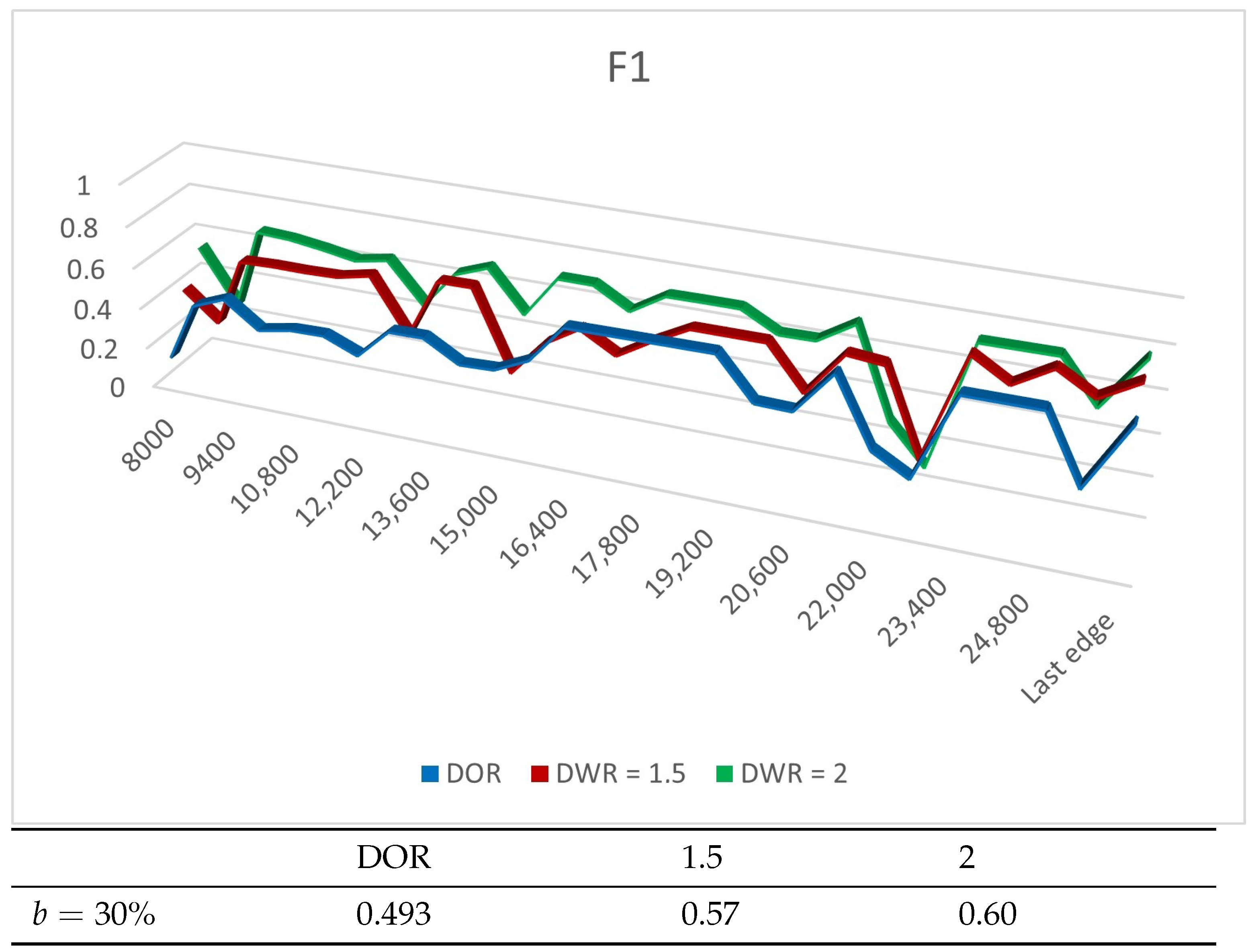
4.4.1. Experiments on Synthetic Datasets
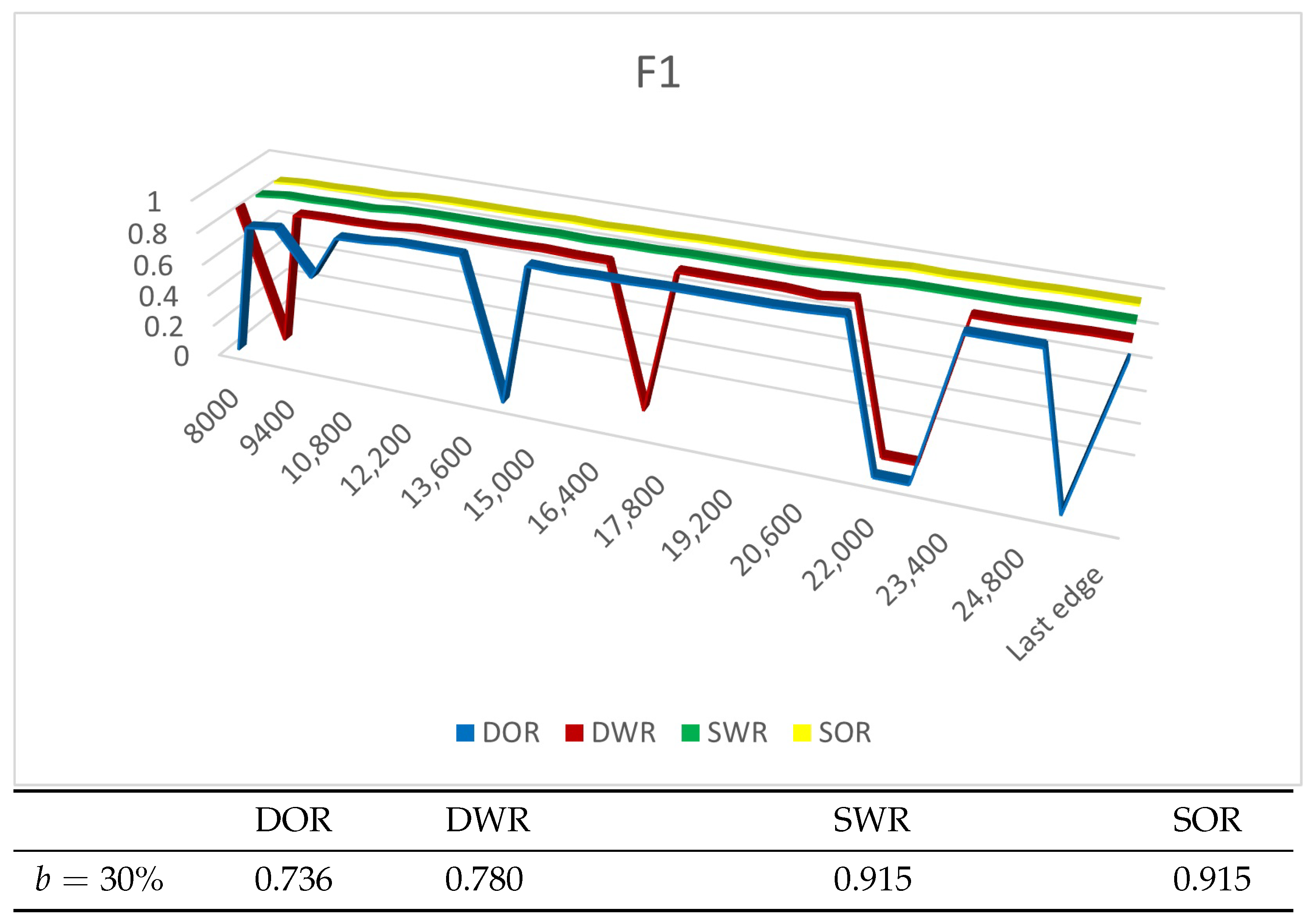
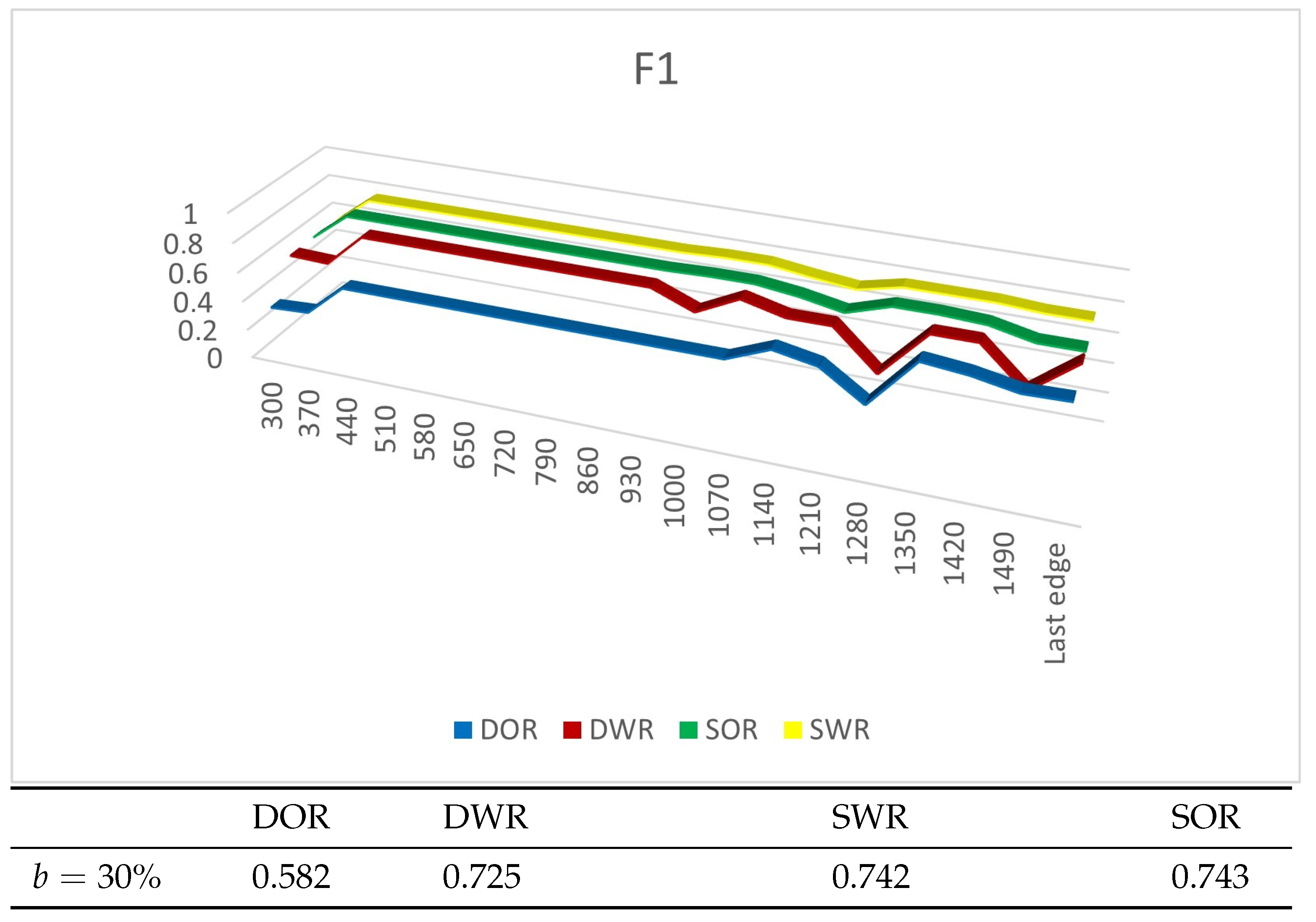
4.4.2. Experiments on Real Datasets
5. Discussion
6. Conclusions
Author Contributions
Funding
Data Availability Statement
Conflicts of Interest
References
- Fortunato, S. Community detection in graphs. Phys. Rep. 2010, 486, 75–174. [Google Scholar] [CrossRef]
- Veldt, N.; Klymko, C.; Gleich, D.F. Flow-based local graph clustering with better seed set inclusion. In Proceedings of the 2019 SIAM International Conference on Data Mining, Calgary, AL, Canada, 2–4 May 2019; pp. 378–386. [Google Scholar]
- Bian, Y.; Ni, J.; Cheng, W.; Zhang, X. The multi-walker chain and its application in local community detection. Knowl. Inf. Syst. 2019, 60, 1663–1691. [Google Scholar] [CrossRef]
- Bian, Y.; Luo, D.; Yan, Y.; Cheng, W.; Wang, W.; Zhang, X. Memory-based random walk for multi-query local community detection. Knowl. Inf. Syst. 2020, 62, 2067–2101. [Google Scholar] [CrossRef]
- De Meo, P.; Ferrara, E.; Fiumara, G.; Provetti, A. Mixing local and global information for community detection in large networks. J. Comput. Syst. Sci. 2014, 80, 72–87. [Google Scholar] [CrossRef]
- Baltsou, G.; Christopoulos, K.; Tsichlas, K. Local Community Detection: A Survey. IEEE Access 2022, 10, 110701–110726. [Google Scholar] [CrossRef]
- Kostakos, V. Temporal graphs. Phys. A Stat. Mech. Its Appl. 2009, 388, 1007–1023. [Google Scholar] [CrossRef]
- Casteigts, A.; Flocchini, P.; Quattrociocchi, W.; Santoro, N. Time-varying graphs and dynamic networks. In Proceedings of the 10th International Conference, ADHOC-NOW 2011, Paderborn, Germany, 18–20 July 2011; Springer: Berlin/Heidelberg, Germany, 2011; pp. 346–359. [Google Scholar]
- Baltsou, G.; Tsichlas, K. Dynamic Community Detection with Anchors. In Proceedings of the 10th International Conference on Complex Networks and Their Applications, Madrid, Spain, 30 November–2 December 2021; Published by the International Conference on Complex Networks and Their Applications. pp. 64–67. [Google Scholar]
- Yang, L.; Shami, A. IoT data analytics in dynamic environments: From an automated machine learning perspective. Eng. Appl. Artif. Intell. 2022, 116, 105366. [Google Scholar] [CrossRef]
- Bonifazi, G.; Cauteruccio, F.; Corradini, E.; Marchetti, M.; Terracina, G.; Ursino, D.; Virgili, L. A framework for investigating the dynamics of user and community sentiments in a social platform. Data Knowl. Eng. 2023, 146, 102183. [Google Scholar] [CrossRef]
- Bonifazi, G.; Cecchini, S.; Corradini, E.; Giuliani, L.; Ursino, D.; Virgili, L. Investigating community evolutions in TikTok dangerous and non-dangerous challenges. J. Inf. Sci. 2022, 2022, 01655515221116519. [Google Scholar] [CrossRef]
- Jalabneh, R.; Syed, H.Z.; Pillai, S.; Apu, E.H.; Hussein, M.R.; Kabir, R.; Arafat, S.Y.; Majumder, M.A.A.; Saxena, S.K. Use of mobile phone apps for contact tracing to control the COVID-19 pandemic: A literature review. Appl. Artif. Intell. COVID-19 2021, 2021, 389–404. [Google Scholar]
- Radanliev, P.; De Roure, D.; Ani, U.; Carvalho, G. The ethics of shared COVID-19 risks: An epistemological framework for ethical health technology assessment of risk in vaccine supply chain infrastructures. Health Technol. 2021, 11, 1083–1091. [Google Scholar] [CrossRef]
- Radanliev, P.; De Roure, D. Epistemological and bibliometric analysis of ethics and shared responsibility—Health policy and IoT systems. Sustainability 2021, 13, 8355. [Google Scholar] [CrossRef]
- Aggarwal, C.C.; Yu, P.S. Online analysis of community evolution in data streams. In Proceedings of the 2005 SIAM International Conference on Data Mining, Beach, CA, USA, 21–23 April 2005; pp. 56–67. [Google Scholar]
- Duan, D.; Li, Y.; Jin, Y.; Lu, Z. Community mining on dynamic weighted directed graphs. In Proceedings of the 1st ACM International Workshop on Complex Networks Meet Information & Knowledge Management, Hong Kong, China, 2–6 November 2009; pp. 11–18. [Google Scholar]
- Takaffoli, M.; Rabbany, R.; Zaïane, O.R. Incremental local community identification in dynamic social networks. In Proceedings of the 2013 IEEE/ACM International Conference on Advances in Social Networks Analysis and Mining (ASONAM 2013), Istanbul, Turkey, 10–13 November 2013; pp. 90–94. [Google Scholar]
- Chen, J.; Zaiane, O.R.; Goebel, R. Detecting communities in large networks by iterative local expansion. In Proceedings of the 2009 International Conference on Computational Aspects of Social Networks, Fontainebleau, France, 24–27 June 2009; pp. 105–112. [Google Scholar]
- Yun, S.Y.; Proutiere, A. Streaming, memory limited algorithms for community detection. Adv. Neural Inf. Process. Syst. 2014, 27, 3167–3175. [Google Scholar]
- Zakrzewska, A.; Bader, D.A. A dynamic algorithm for local community detection in graphs. In Proceedings of the 2015 IEEE/ACM International Conference on Advances in Social Networks Analysis and Mining (ASONAM), Paris, France, 25–28 August 2015; pp. 559–564. [Google Scholar]
- Zakrzewska, A.; Bader, D.A. Tracking local communities in streaming graphs with a dynamic algorithm. Soc. Netw. Anal. Min. 2016, 6, 65. [Google Scholar] [CrossRef]
- Kanezashi, H.; Suzumura, T. An incremental local-first community detection method for dynamic graphs. In Proceedings of the 2016 IEEE International Conference on Big Data (Big Data), Washington, DC, USA, 5–8 December 2016; pp. 3318–3325. [Google Scholar]
- Coscia, M.; Rossetti, G.; Giannotti, F.; Pedreschi, D. Demon: A local-first discovery method for overlapping communities. In Proceedings of the 18th ACM SIGKDD International Conference on Knowledge Discovery and Data Mining, Beijing, China, 12–16 August 2012; pp. 615–623. [Google Scholar]
- DiTursi, D.J.; Ghosh, G.; Bogdanov, P. Local community detection in dynamic networks. In Proceedings of the 2017 IEEE International Conference on Data Mining (ICDM), New Orleans, LA, USA, 18–21 November 2017; pp. 847–852. [Google Scholar]
- Guo, K.; He, L.; Huang, J.; Chen, Y.; Lin, B. A Local Dynamic Community Detection Algorithm Based on Node Contribution. In Proceedings of the CCF Conference on Computer Supported Cooperative Work and Social Computing, Kunming, China, 16–18 August 2019; Springer: Berlin/Heidelberg, Germany, 2019; pp. 363–376. [Google Scholar]
- Conde-Cespedes, P.; Ngonmang, B.; Viennet, E. An efficient method for mining the maximal α-quasi-clique-community of a given node in complex networks. Soc. Netw. Anal. Min. 2018, 8, 20. [Google Scholar] [CrossRef]
- Liu, J.; Shao, Y.; Su, S. Multiple local community detection via high-quality seed identification over both static and dynamic networks. Data Sci. Eng. 2021, 6, 249–264. [Google Scholar] [CrossRef]
- Liakos, P.; Papakonstantinopoulou, K.; Ntoulas, A.; Delis, A. Rapid detection of local communities in graph streams. IEEE Trans. Knowl. Data Eng. 2020, 34, 2375–2386. [Google Scholar] [CrossRef]
- Rossetti, G.; Cazabet, R. Community discovery in dynamic networks: A survey. ACM Comput. Surv. (CSUR) 2018, 51, 1–37. [Google Scholar] [CrossRef]
- Havemann, F.; Heinz, M.; Struck, A.; Gläser, J. Identification of overlapping communities and their hierarchy by locally calculating community-changing resolution levels. J. Stat. Mech. Theory Exp. 2011, 2011, P01023. [Google Scholar] [CrossRef]
- Rossetti, G. RDYN: Graph benchmark handling community dynamics. J. Complex Netw. 2017, 5, 893–912. [Google Scholar] [CrossRef]
- Collection, Stanford Large Network Dataset. Available online: http://snap.stanford.edu/data (accessed on 25 November 2022).
- Database, J.J.A.T.T. Al Qaeda Operations Attack Series 1993–2003, Worldwide. 2003. Available online: http://doitapps.jjay.cuny.edu/jjatt/data.php (accessed on 5 November 2022).
- F1 Score Lemma. F1 Score Lemma—Wikipedia, the Free Encyclopedia. Available online: https://en.wikipedia.org/wiki/F-score (accessed on 5 May 2022).
- Li, Y.; He, K.; Bindel, D.; Hopcroft, J.E. Uncovering the small community structure in large networks: A local spectral approach. In Proceedings of the 24th International Conference on World Wide Web, Florence, Italy, 18–22 May 2015; pp. 658–668. [Google Scholar]
- Li, Y.; He, K.; Kloster, K.; Bindel, D.; Hopcroft, J. Local spectral clustering for overlapping community detection. ACM Trans. Knowl. Discov. Data (TKDD) 2018, 12, 1–27. [Google Scholar] [CrossRef]
- Shang, R.; Zhang, W.; Zhang, J.; Feng, J.; Jiao, L. Local community detection based on higher-order structure and edge information. Phys. A Stat. Mech. Its Appl. 2022, 587, 126513. [Google Scholar] [CrossRef]
- Rossetti, G.; Pappalardo, L.; Rinzivillo, S. A novel approach to evaluate community detection algorithms on ground truth. In Proceedings of the Complex Networks VII: Proceedings of the 7th Workshop on Complex Networks CompleNet 2016, Dijon, France, 23–25 March 2016; Springer: Berlin/Heidelberg, Germany, 2016; pp. 133–144. [Google Scholar]
- Zhang, Y.; Wu, B.; Liu, Y.; Lv, J. Local community detection based on network motifs. Tsinghua Sci. Technol. 2019, 24, 716–727. [Google Scholar] [CrossRef]
- Jaccard Similarity Coefficient Lemma. Jaccard Similarity Coefficient Lemma—Wikipedia, the Free Encyclopedia. Available online: https://en.wikipedia.org/wiki/Jaccard_index (accessed on 2 November 2022).
- Labatut, V.; Cherifi, H. Accuracy measures for the comparison of classifiers. arXiv 2012, arXiv:1207.3790. [Google Scholar]
- Bharali, A. An Analysis of Email-Eu-Core Network. Int. J. Sci. Res. Math. Stat. Sci. 2018, 5, 100–104. [Google Scholar] [CrossRef]
- Gill, P.; Young, J.K. Comparing Role-Specific Terrorist Profiles. 2011. SSRN 1782008. Available online: https://papers.ssrn.com/sol3/papers.cfm?abstract_id=1782008 (accessed on 8 November 2022).
- Gao, Y.; Zhang, H.; Zhang, Y. Overlapping community detection based on conductance optimization in large-scale networks. Phys. A Stat. Mech. Its Appl. 2019, 522, 69–79. [Google Scholar] [CrossRef]


| Symbol/Abbreviation | Description |
|---|---|
| The network at time instance t—if no time index is given (G) then time is irrelevant | |
| V | The node set of G |
| N | The total number of nodes in G () |
| The edge set of network G at time t | |
| Weight of edge e | |
| A | The anchor node |
| The community of the anchor at time t | |
| The total internal degree of , when the i-th node is inserted to the community | |
| The total boundary degree of , when the i-th node is inserted to the community C | |
| The set of neighbors of node u | |
| R | The radius of the ball centered around the anchor A |
| The set of nodes, called influence range, in distance at most R from anchor A. | |
| The streaming source | |
| b | The size of the batch in the streaming algorithm |
| LCDS-A | The proposed General framework of Local Community detection in graph streams with Anchors |
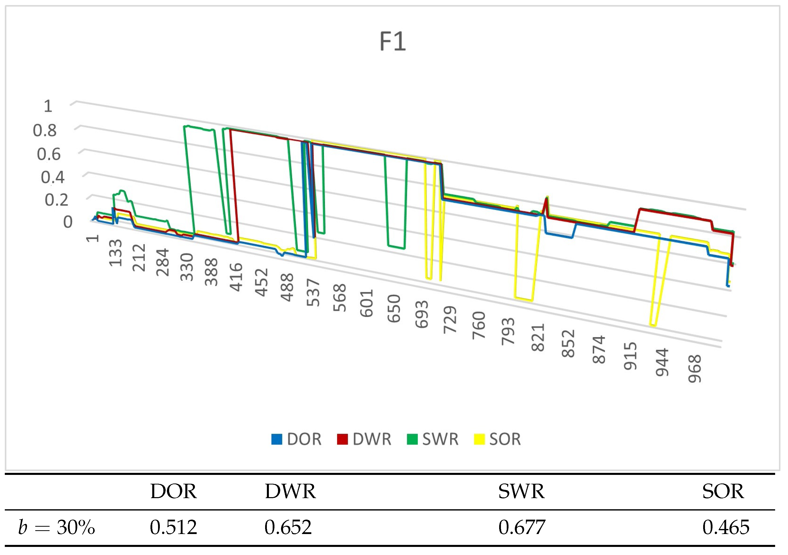
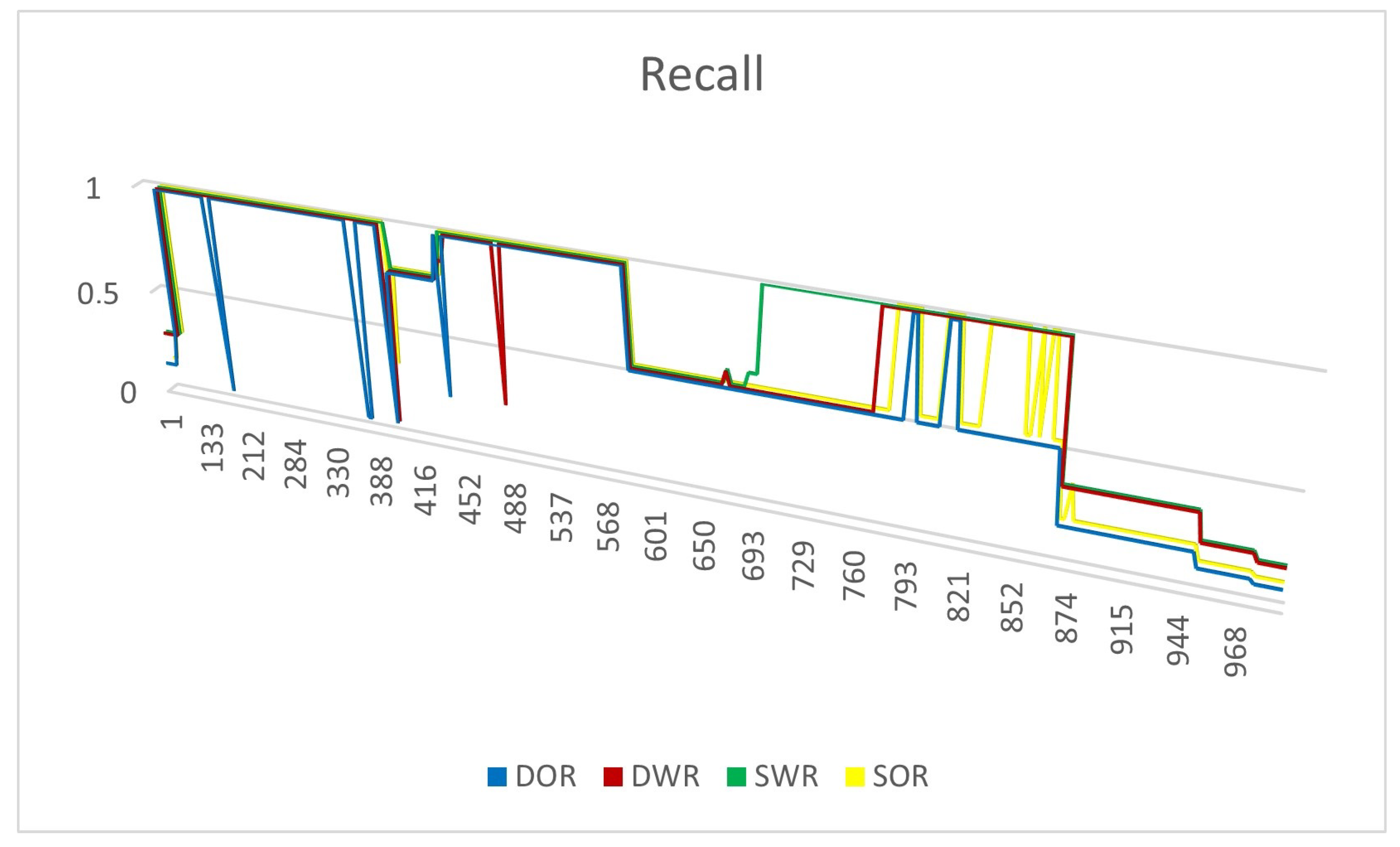
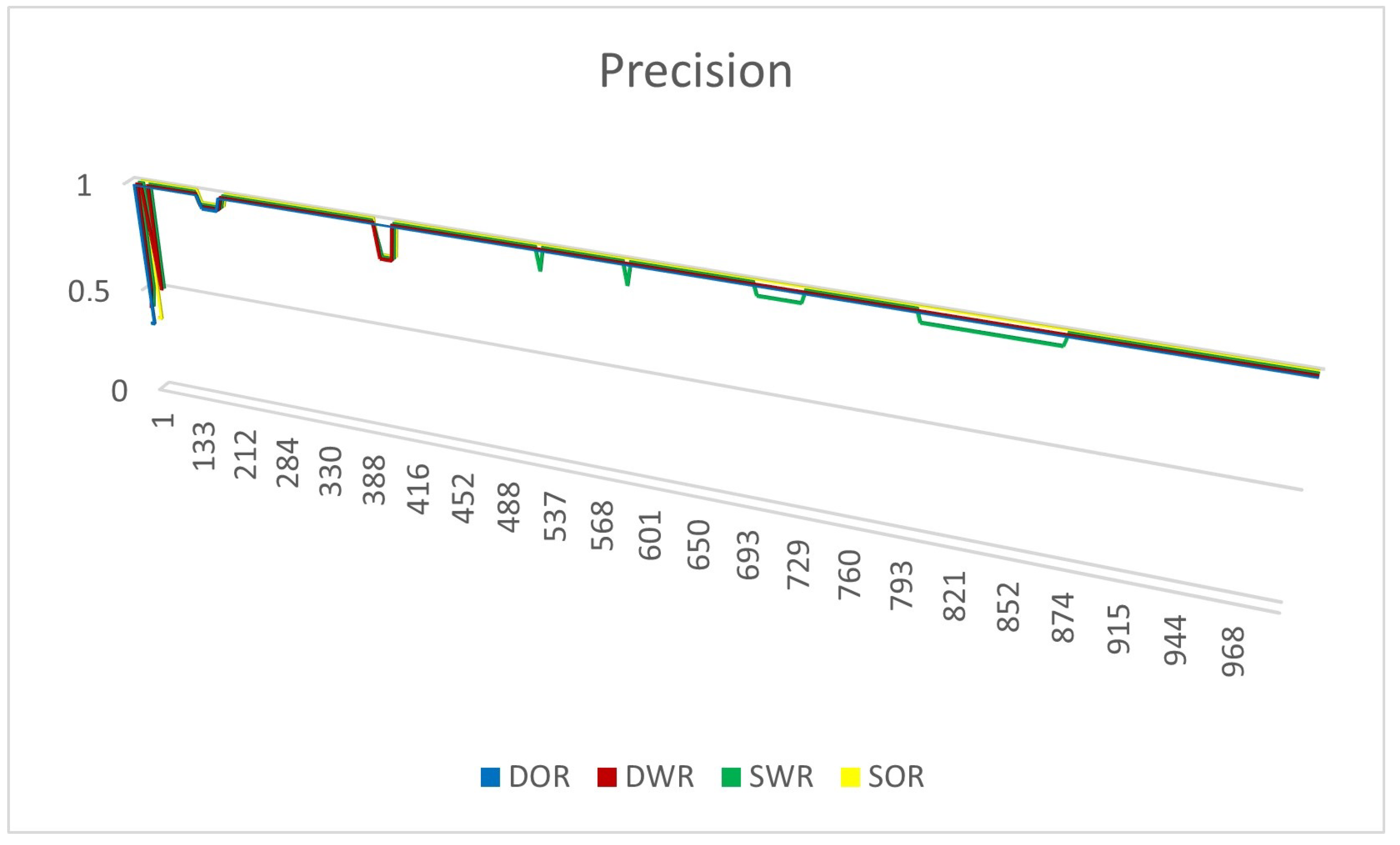
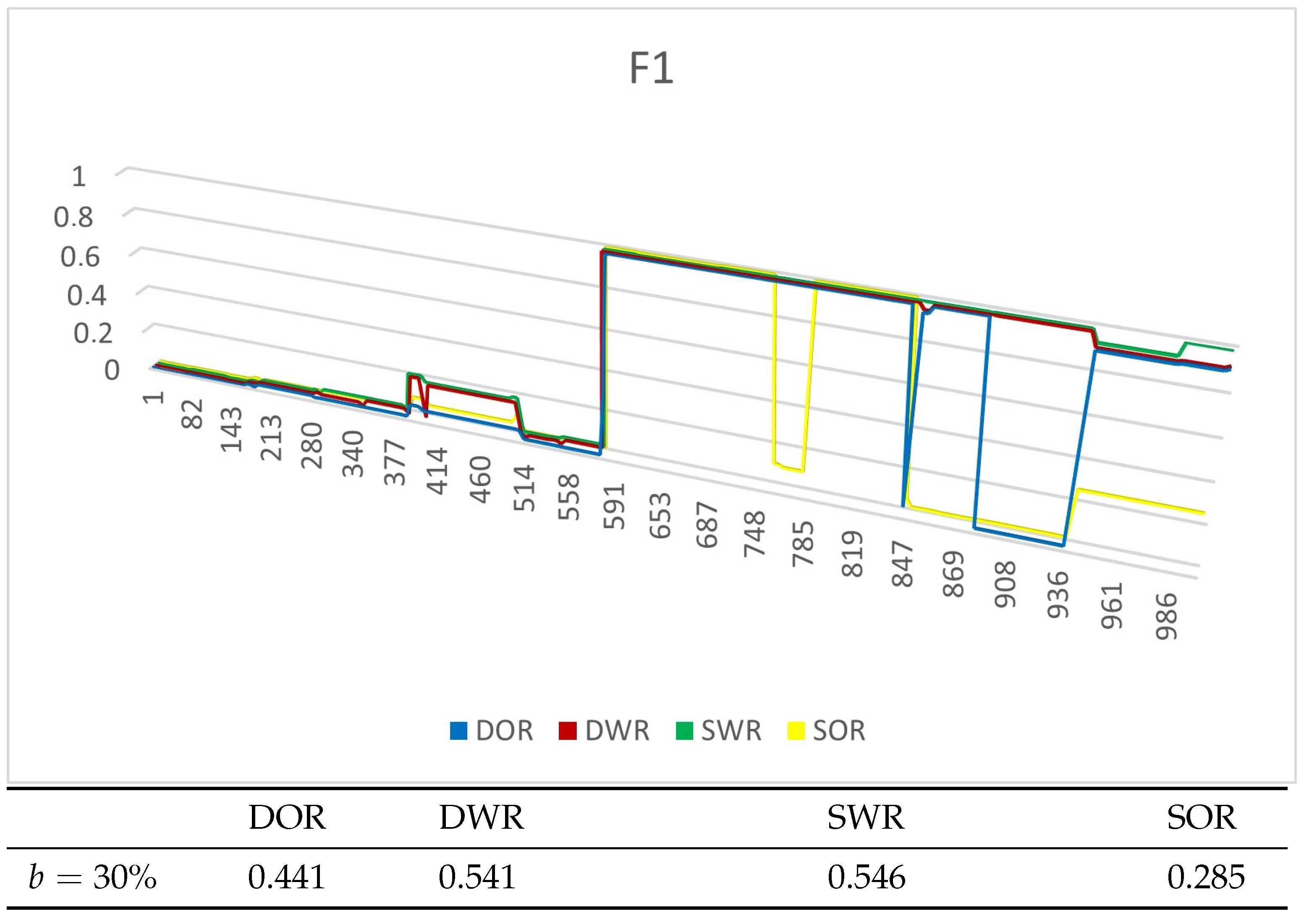
| DWR | The Dynamic With Rewards algorithm. It is an instance of LCDS-A for a particular reward scheme and quality metric. |
| DOR | The Dynamic WithOut Rewards algorithm [22] |
| SWR | The Static With Rewards algorithm |
| SOR | The Static withOut Rewards algorithm |
| Sequence of added nodes | A | … | |||
| Incremental Community Sequence | … | ||||
| Internal edges of | … | ||||
| Boundary edges of | … | ||||
| Fitness scores in ascending order | … |
| Dataset | Nodes | Mean Degree | Iterations | Final Edges | Stream Updates |
|---|---|---|---|---|---|
| 500 | 64 | 1000 | 1680 | 41,433 | |
| 1000 | 54 | 1000 | 6226 | 50,871 | |
| 5000 | 55 | 1000 | 25,590 | 251,107 |
| Dataset | Nodes | Actions |
|---|---|---|
| 271 | 756 | |
| 1006 | 16,706 |
| DOR | Time | 2 | 3 | 5 | 10 | Time | |||
|---|---|---|---|---|---|---|---|---|---|
| s | s | ||||||||
| s | s | ||||||||
| s | s | ||||||||
| s | s |
Disclaimer/Publisher’s Note: The statements, opinions and data contained in all publications are solely those of the individual author(s) and contributor(s) and not of MDPI and/or the editor(s). MDPI and/or the editor(s) disclaim responsibility for any injury to people or property resulting from any ideas, methods, instructions or products referred to in the content. |
© 2023 by the authors. Licensee MDPI, Basel, Switzerland. This article is an open access article distributed under the terms and conditions of the Creative Commons Attribution (CC BY) license (https://creativecommons.org/licenses/by/4.0/).
Share and Cite
Christopoulos, K.; Baltsou, G.; Tsichlas, K. Local Community Detection in Graph Streams with Anchors. Information 2023, 14, 332. https://doi.org/10.3390/info14060332
Christopoulos K, Baltsou G, Tsichlas K. Local Community Detection in Graph Streams with Anchors. Information. 2023; 14(6):332. https://doi.org/10.3390/info14060332
Chicago/Turabian StyleChristopoulos, Konstantinos, Georgia Baltsou, and Konstantinos Tsichlas. 2023. "Local Community Detection in Graph Streams with Anchors" Information 14, no. 6: 332. https://doi.org/10.3390/info14060332
APA StyleChristopoulos, K., Baltsou, G., & Tsichlas, K. (2023). Local Community Detection in Graph Streams with Anchors. Information, 14(6), 332. https://doi.org/10.3390/info14060332