1. Introduction
Moore’s law states that “every 24 months, the number of transistors that can be placed on a chip doubles” [
1]. Of course, keeping up with Moore’s law is a very difficult task as it requires continuous improvement in an already very advanced field. Despite this, recent advances in the integrated circuits (ICs) manufacturing process and specifically in photolithography enable the community to be able to meet this very strict requirements. Photolithography [
2] is a very important part of the whole process because it is responsible for transferring a desired pattern to a photosensitive material on the wafer surface (photo-curable material; most typically, commercial photo resistance [
3]) by exposing it to ultraviolet (UV) or extreme-UV (EUV) light. Successful photolithography will yield wafers with a high overlay (OVL) and a small critical dimension (CD). OVL and CD are the key performance indicators (KPIs) for the photolithography stage. Overlay is a measure of the correct alignment between the various layers of the wafer and CD is known as the minimum feature size which refers to the width of the lines, spaces, contact holes or dots of critical circuit patterns. The better the OVL and the smaller the CD, the smaller the exposed pattern and of course the smaller the exposed ICs on the wafer. This is why photolithography is the most important stage of the ICs fabrication process. This is the stage that drives Moore’s law.
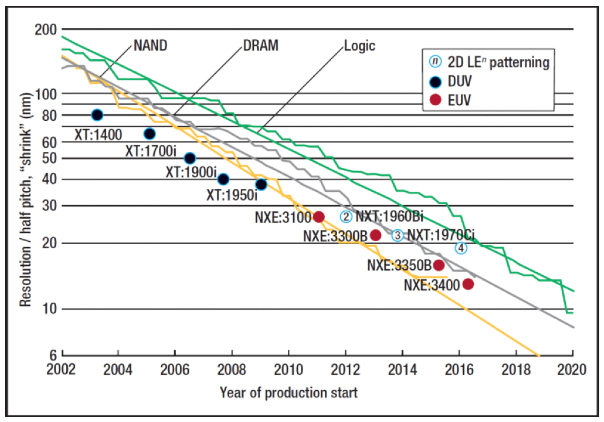
EUV photolithography, a technology entirely unique to ASML, is the state of the art (SoA) in photolithography and the stepping stone to keep up with Moore’s law. EUV light’s wavelength is at 13.5 nanometers, i.e., 14 times shorter than DUV light, and is a key enabler for small CD and better OVL. Hence, from 2010 onwards, the EUV platforms (NXE) of ASML lead the race of keeping up with Moore’s law. In
Figure 1, we see a visualization of Moore’s law in terms of chip shrinkage together the photolithography machines that achieve these results as well.
In
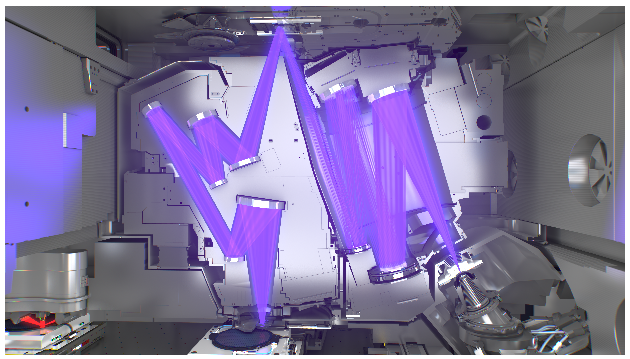
Figure 2, the full light path from the EUV source to the silicon wafer is presented. The light is generated in the source, sent into the illuminator which controls the light beam, reflects off the mask with the chip pattern, before being focused in the projection optics and exposing the wafer. The projection optics box of the EUV machine, which actually consists of mirrors, is responsible for directing EUV light on the wafer surface. Ideally, the wavefront of the light reaches the wafer surfaces without any optical imperfections. This would expose a perfect wafer but of course this is almost never the case.
Platforms for new products such the one of ASML in
Figure 3 are built on these breakthroughs. Platforms that are able to produce wafers with high performance (throughput), high precision at the nanometer level (overlay), and optimized imaging capabilities (focus and critical dimension uniformity) [
4].
Photolithography machines are some of the most complex machines in terms of hardware and software that exist in the industry. With more than fifty million lines of code-base and thousands of hardware modules, being able to orchestrate and control the machine such that it meets the extremely strict OVL and CD requirements is a very difficult task. Hardware itself cannot achieve such perfection. For this reason, a vital part of the machine is software control algorithms which deal with any kind of hardware imperfections. Software will enable the machine to meet the OVL and CD KPIs which will verify the quality of the machine. In principle, the main idea behind this is that the machine is able to model accurately, at the nanometer level, the expected wavefront anomalies. Then, by knowing what to expect, software will optimize the corresponding knobs on the machine, such as mirror positions, for example, such that it compensates for the expected aberrations. In that case, the expected fingerprint will be corrected before reaching the wafer surface, which means that the desired pattern will be exposed with minimum imperfections. In this case, we understand that being able to build accurate models is one of the most crucial and demanding tasks for the photolithography process. These models are the key enablers for a successful exposure.
Building such models, however, is also very time costly. During the model creation phase several sensor measurements are needed. These measurements will serve as a reference and the model parameters will be optimized based on them. Of course, the more the measurements, the bigger the accuracy, however, we are then against the throughput vs. quality trade-off. As mentioned above, throughput, in terms of wafers per hour (wph), is also very important and chip manufacturers cannot afford any throughput loss on the photolithography process. Usually, the number of points to measure is predetermined by the time budget of the process. Then, we are called to find which points to measure such that the measurements in those points will provide the maximum amount of information needed to optimize the models. Hence, we are called to solve this specific optimization problem, namely that of how the best subset of points can be selected to measure out of a set of available locations on the wafer surface, in order to obtain maximum information regarding the fingerprint estimation model without introducing a significant throughput loss. This is a typical optimal experimental design (OED) problem.
The optimal experimental design (OED) problem has been a center of interest of both academia and industry for a very long time already. Since the first scientific paper on this topic was published by Smith in 1918 [
6] and to this day, after numerous papers and research in this field, advances in this area are quite remarkable. In our paper, as mentioned above, we examine a certain application of OED in the photolithographic process. OED problems can be linear or nonlinear based on the model nature. Nonlinear models need to be solved with heuristic approaches. However, heuristics are not optimal, especially for complex systems with high dimensionality, nonlinear responses and dynamics, multiphysics, and uncertain and noisy environments. OED for linear models [
7,
8], on the other hand, are using criteria based on the information matrix derived by the model. These criteria can be analytically calculated and are different flavors of the dispersion of that matrix. The so-called Fisher-based criteria comprise G-, D-, and A-optimality. The disadvantage of this approach, however, is that most of these algorithms are greedy and most of the times are not optimal. In this paper, we are proposing a hybrid method incorporating both a deterministic part and a meta-heuristic genetic algorithm (GA)-based part. On the one hand, the stochasticity of GA can compensate for the greedy approach of the first step, and on the other hand, the GA can identify hidden patterns in the combination of good solutions created previously and exploit this information for creating the final solution. This innovative solution in combination with the real life use case from the industry serves as a promising alternative for similar problems.
An outline of the rest of this paper is as follows.
Section 2 addresses the formulation problem discussing the theory and basic concepts of the OED problem on the one hand, and presents the specific photolithographic OED use case on the other. In
Section 3, the proposed solution is presented, and
Section 4 exhibits the results of our solution. Finally,
Section 5 elaborates upon the conclusions and the future work.
2. Problem Formulation
2.1. Optimal Experimental Design (OED)
An experiment is a process carried out under carefully controlled conditions in order to establish some kind of knowledge on a specific topic. This knowledge is expressed by a model, which is the key element of an experiment. The model is related to the experimental responses, or to the experimental observations, or to the corresponding experimental factors. The purpose of the experiment itself is to define an accurate model. Experiments are designed to optimize the parameters of a model or for estimating the responses of an already fitted model. In this paper, we are interested in optimizing the parameters of an OVL model, for example. An optimally designed experiment, in this case, will provide the maximum information in the most efficient way in order to gain knowledge about the model.
Even under the most protected laboratory environment, however, it is often not possible to avoid random experimental errors. Such errors can either be small and harmless or can also be catastrophic for the experiments under certain conditions of noisy experiments or highly dimensional models, for example. For this reason, statistical methods are essential for the optimal design and analysis of the experiment, such that these will provide the maximum amount of information independently of those error factors. Optimal experimental design (OED) is a field between mathematics and computer science, which deals with this specific topic of designing optimal experiments exploiting various statistical methods.
In OED problems, the key input is the model. OED designs either depend on the model to be fitted to the data, or for linear models on the values of the parameters of the models. As mentioned above, the model is describing the relation between the observed response Y and the experimental factors X. Depending on the use case, models can be linear or nonlinear. In this paper, linear polynomial models are examined. More specifically, let us consider the linear model with:
- 1.
Y being an N-component column of experimental observations;
- 2.
X being an matrix of known elements known as information matrix;
- 3.
b being a vector of size p of unknown parameters;
- 4.
being an N component vector of residuals with and , where E and D stand for the expectation operator and dispersion matrix, respectively.
As mentioned above, the goal of the whole experiment is to build a model that is as close as possible to reality. From the above model, the information matrix X is the only known input. The information matrix is in reality the basis functions of the model polynomial. During the process of model selection, the corresponding basis functions are obtained and the information matrix is formed. This process is very interesting, but it is beyond the scope of this paper. In our work, we consider the information matrix X as known. In that case, the unknown parts of the model equation are the b vector of the unknown parameter and the noise . Hence, in order to build our model, our real task is to accurately estimate the parameter vector b.
For parameter estimation, there are different approaches depending on the model that is used. The most common and still very effective one for linear models is the least squares method (LST).
In
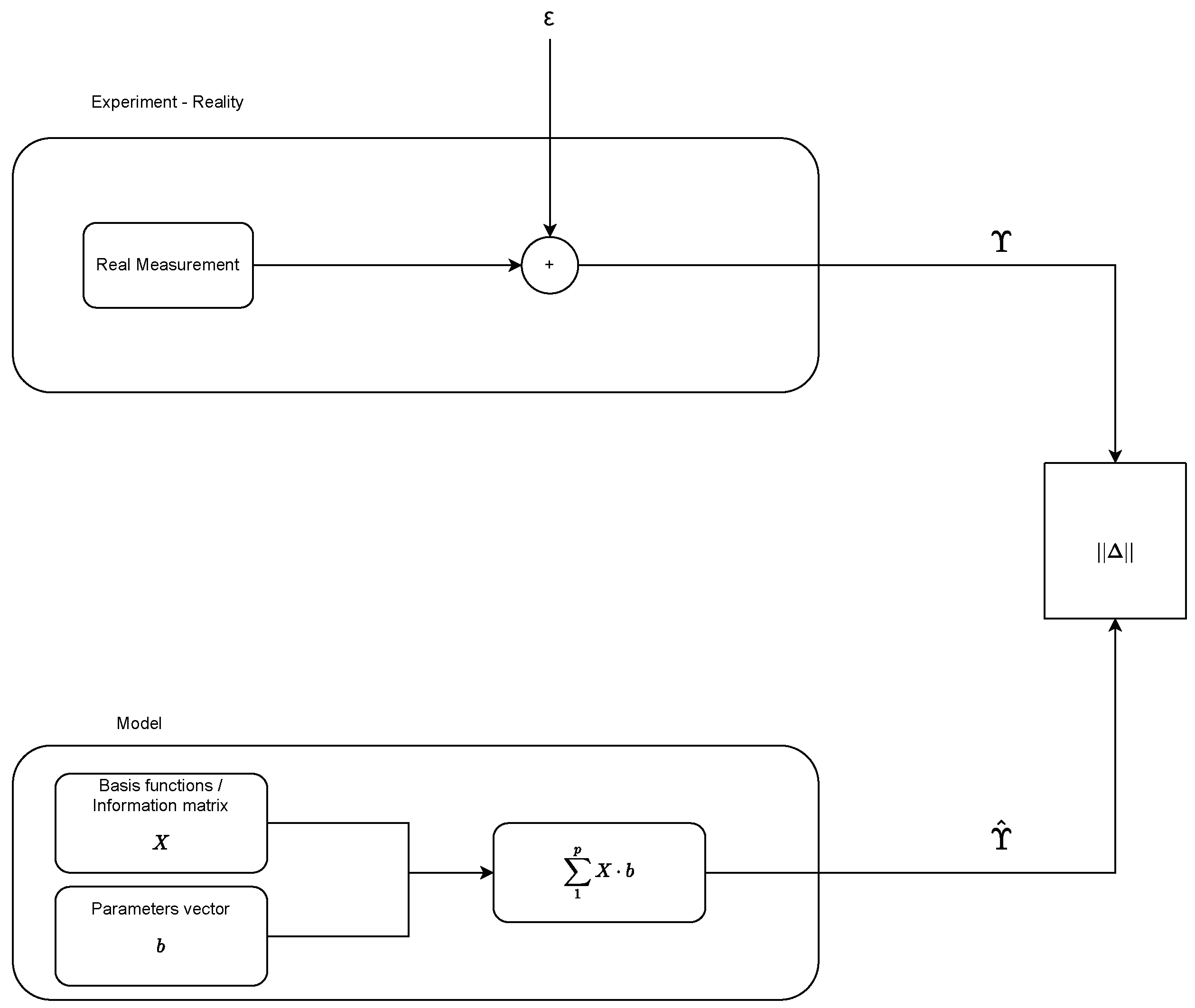
Figure 4, the whole process of parameter estimation is presented. On the top box, the real measurements take place. This is the experiment that takes place. The output of the measurements plus the added noise is the real value
Y. The bottom box contains the modeling part. As we can see, the information matrix
X is already known and does not change throughout the process. On the other hand, the parameters vector
b is the one that gets updated. On the right part of the schema, least squares optimization (LST) takes place. Input to the LST algorithm is the real measurement
Y and the model output
. The output of the LST algorithm will be the update of the parameters vector
b such that the least squares of the differences between
Y and
is minimized. This will mean that the parameters estimates are successful and our model output
is as close to the real measurement of
Y as possible; hence, our model is accurate.
All of this process, however, is highly dependent on the quality of the real measurements performed during the experiment. If the measurements are not informative enough, then the output of the LST algorithm is also not trustworthy. And, this results in a bad model despite the rest of the process working fine. Additionally, in most of the use cases, there is only a limited budget of “experiments” that can be performed. Here, by experiment, we mean one measurement. In this case, the problem of selecting the most informative subset of available measurements is crucial for the success of the process. Hence, the optimal design of the experiment is vital for ensuring the quality of the whole process of model optimization. The OED problem is defined as selecting an n-point design of a set of N candidate points to optimize for a certain design criterion. In most of the OED problems, as already mentioned above, we assume that we have:
- 1.
A given model;
- 2.
An optimality criterion;
- 3.
A fixed sample size of n-points out of a candidate set of N-points.
And, the problem is how to take
n independent observations of the given design space (candidate points). The solution of this problem is the optimal experiment design (OED) which maximizes the confidence in the selected model parameters for providing maximum information [
9]. Optimal designs can be (a) approximate or (b) the exact optimal designs. Approximate designs are obviously easier to extract since they are probability measures defined on a compact and known design space (set of
N candidate points) [
10]. This optimization problem finds the optimal probability measure in terms of a certain design criterion. The design criterion should reflect the amount of information gained if a certain experimental design is chosen.
2.3. Fingerprint Estimation in Photolithography Process Use Case
As mentioned before, the most important KPIs for a photolithography machine are overlay (OVL) and critical dimension (CD). OVL is a critical parameter in photolithography as it determines the alignment accuracy between the different layers being printed on the wafer. Overlay errors can result in misregistration between the different layers, which can cause defects in the final device and reduce the yield. Critical dimension (CD) is another important parameter in photolithography that refers to the size of the features being printed on the wafer. CD control is important because variations in CD can have a significant impact on the performance and yield of the final device.
In photolithography, fingerprint estimation (FE) refers to the process of characterizing the spatial variations in the critical dimensions (CDs) and overlay (OVL) of the features being printed. These variations can arise from a variety of sources, such as imperfections in the mask or in the lithography process itself. Fingerprint estimation is typically performed using specialized metrology tools that can measure the CDs and OVL of the features at various locations on the wafer. The resulting data are then analyzed to extract information about the spatial variations in the CD and OVL, which can be used to create a “fingerprint” of the lithography process. A vital part of the FE process involves the modeling of the OVL and CD. OVL and CD modeling involves developing mathematical and statistical models to predict the impact of different process parameters on OVL and CDs. These models can be used to optimize the lithography process by adjusting the process parameters in real time to achieve the desired OVL and CD specifications. Overall, fingerprint estimation is an important tool in photolithography for ensuring the high yield and consistent performance of the lithography process.
A model in general, and of course also OVL and CD models, is a mathematical or statistical representation of a system or process, a polynomial. A model consists of two key components: basis functions and parameters. The choice of basis functions depends on the nature of the problem and the characteristics of the data being modeled. Parameters of the model on the other hand, are the values that are estimated from the data and are used to define the model. The parameters determine the specific values of the basis functions that best fit the data.
In our specific use case, we need to provide the model for OVL. A linear model
is used for our purposes.
is the information matrix which consists of the basis function
and
p are the parameters of our model. In the expanded version of the model below, each row corresponds to a certain point on the wafer surface. The first row, for example, describes the OVL in point
. Hence, as we can see, the wafer consists of
N available points on which we can measure. Furthermore, the OVL polynomial has
P coefficients or parameters. As described above, the information matrix
is already known to us, and in that case, the goal of FE is to estimate the parameters
p of our model.
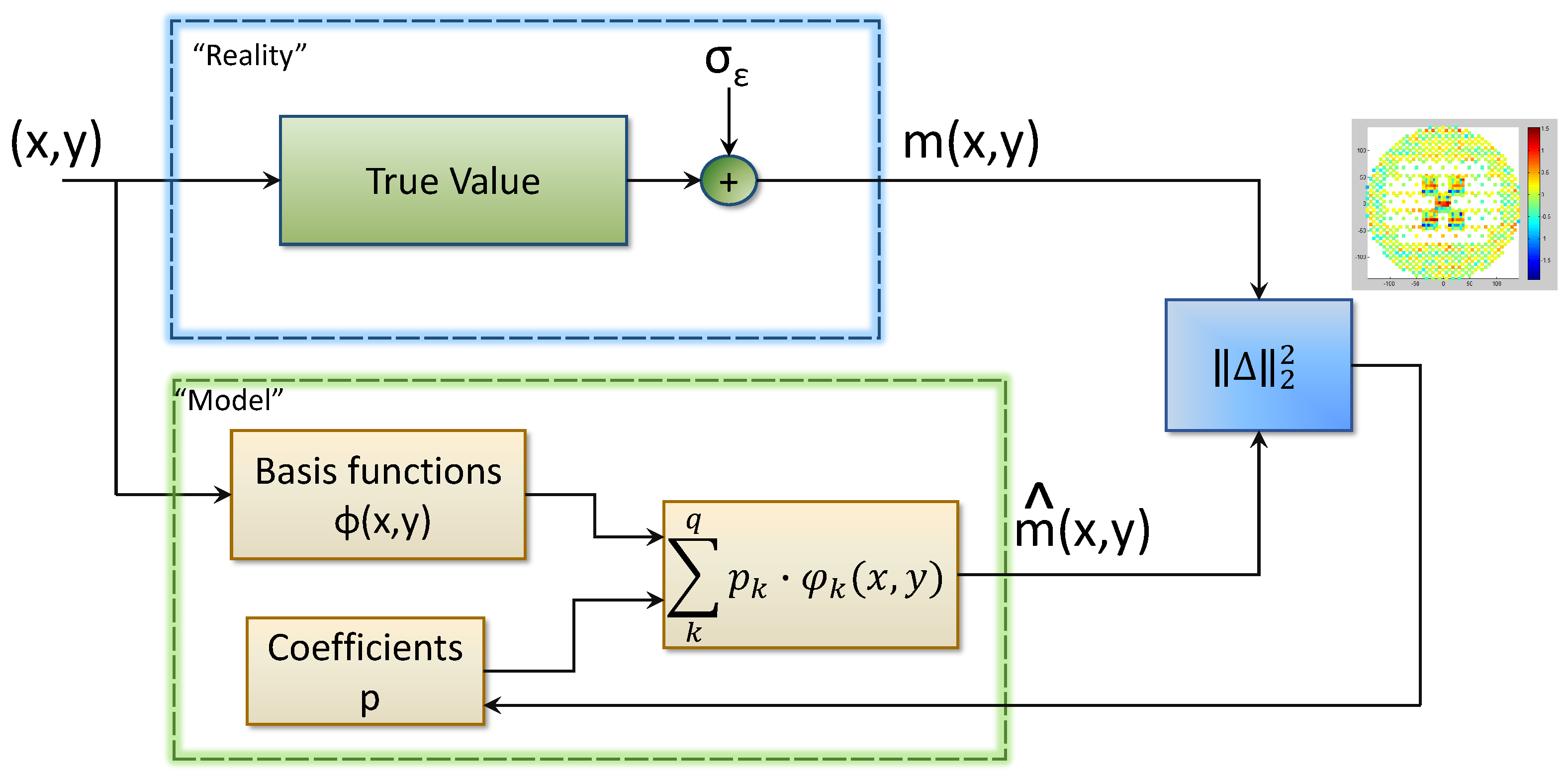
In
Figure 5, the process of FE is presented. Since the basis functions of the model
are already predefined, the goal of the FE process is to obtain the best estimation of the model parameters
p which are obtained by minimizing the
norm of the “real” measurements
(on the top part of
Figure 5) and the “modeled” results
, the least squares optimization (LST). In this case, the inputs to the least squares algorithm are
and
and the output is the update to the coefficients.
However, one of the key parts of the process is obtaining the real measurements . The quality of these measurements can directly affect the quality of the FE.
Unfortunately, these sensor measurements are time costly and are significantly affecting the throughput of the photolithography machine. Hence, we do not have the budget to measure all available N points on the wafer. In most cases, the maximum number of measurements that can be performed is a very small subset of the available points. In this case, we need to design our experimental space, i.e., the sensor measurements, such that even the small subset of available measurements can provide the maximum amount of information. Optimal experimental design (OED) can be used to optimize the design of experiments when measuring the wafer surface by selecting an optimal subset n of all the available sampling points N.
Thus, the specific problem that we need to solve is that of how n can be selected out of N points for measuring, such that the measurements will provide us with the maximum amount of information for fine tuning the parameters of our model. In our case, and . Additionally, due to the nature of the problem, we have one constraint. We have to measure around the wafer surface as uniformly as possible and also not sample points that are too close to each other. In the following section, namely that of Materials and Methods, the proposed solution to the above described problem is presented.
3. Materials and Methods
The only information that is available to us at this point is the matrix , i.e., the information matrix. The goal of our algorithm is to provide an NMU design of our OED problem. As mentioned above, NMU can be calculated at any point on the wafer:
NMU optimality, however, is not our only concern. We are also interested in uniformly sampling from the wafer. Hence, our optimality criteria are (1) NMU optimal design and (2) uniform sampling.
In this section, we present a method for solving the optimal experimental design (OED) problem of selecting
out of
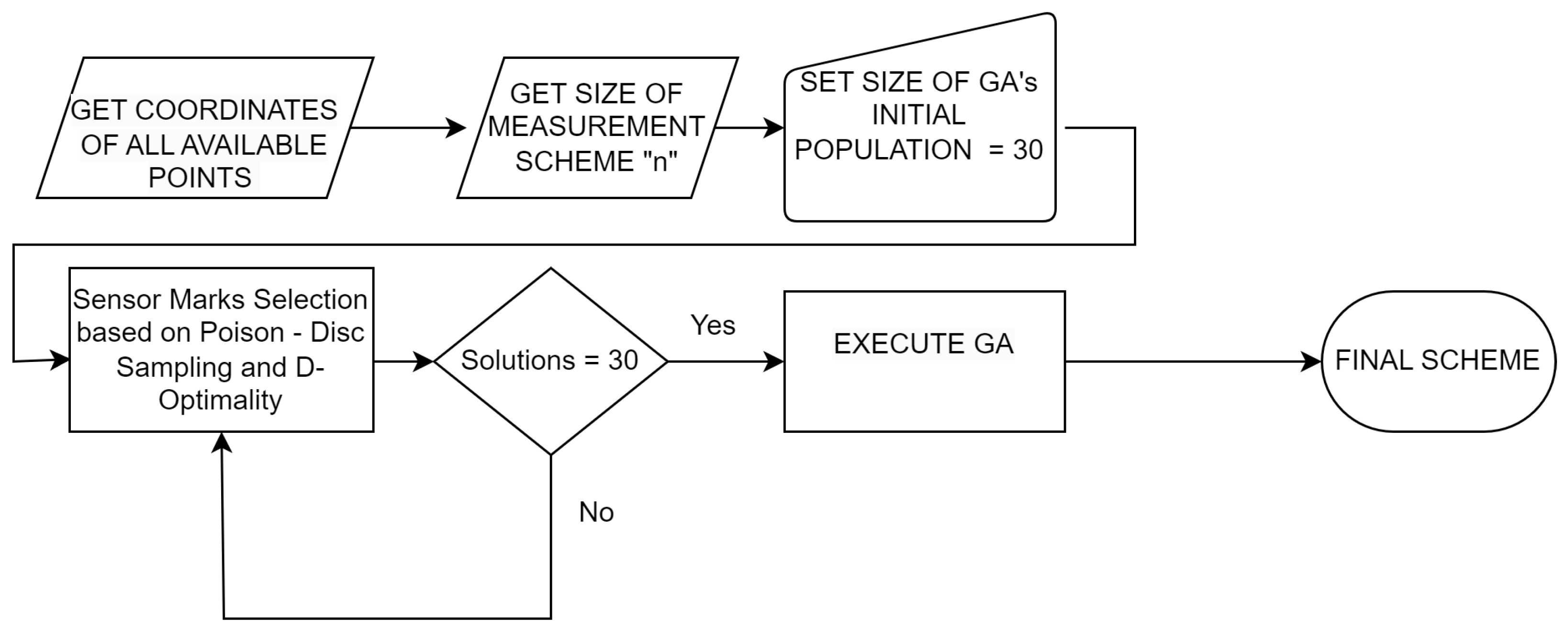
available points on the wafer, which will provide the maximum amount of information to estimate the parameters of the OVL model. The high-level diagram of the genetic algorithm-enhanced sensor mark selection (GAESMS) is presented in
Figure 6.
In the first two blocks, we obtain the input to our OED problem, , and the size of the measurement scheme; in other words, we obtain the budget of our OED problem, . In the following block, we need to determine the size of the initial population of the GA. In our case, we set . In the following blocks, we enter the core functionality of the GAESMS algorithm which will be described in detail in the coming sub-sections.
3.1. Sensor Mark Selection Based on Poisson-Disc Sampling and D-Optimality
In sensor mark selection problems, the goal is to select a subset of points from a larger set of candidate points such that the selected points provide the most informative measurements for a given application. Two important criteria for selecting these points are spatial randomness and sample uniformity. Spatial randomness refers to the evenness of the distribution of the selected points across the area of interest. A spatially random distribution of points helps ensure that the selected points are representative of the entire area, rather than being biased towards certain regions. This is important because biased samples can lead to inaccurate or incomplete measurements, which can ultimately impact the quality and reliability of the application. Sample uniformity, on the other hand, refers to the evenness of the distance between selected points. A uniform distribution of points helps ensure that each point contributes equally to the overall measurement and that the measurements are not biased towards certain areas. This is particularly important in applications where the measured quantity varies significantly across the area of interest, as a non-uniform sample may miss important features or over-represent certain regions.
In summary, both spatial randomness and sample uniformity are critical criteria for selecting sensor marks in order to ensure accurate and representative measurements. By considering these criteria, we can select a subset of points that provides the most informative measurements and improves the overall performance of the application.
In our problem as well, as already mentioned above, instead of only an NMU-based criterion, we also need to provide a uniform design. For this reason, we incorporate Poisson-disc sampling as part of the sensor mark selection algorithm.
Poisson-disc sampling with nearest neighbors is a method used for generating spatially random point sets on a two-dimensional surface [
13,
14]. This technique is particularly useful in sensor mark selection problems, as in our case, where it is essential to ensure both spatial randomness and sample uniformity. The goal is to generate a set of points that cover the area of interest while avoiding overlaps and producing a uniform distribution.
To ensure spatial randomness, the algorithm disqualifies the nearest neighbors of a point as candidate points. Specifically, for each new point, the algorithm checks the nearest neighbors of all existing points and removes them from the list of potential candidate points. This prevents points from being too close to each other and ensures a spatially random distribution. The algorithm continues this process, iteratively selecting new points until the entire surface is covered by a set of non-overlapping discs.
By adjusting the parameters of the algorithm, such as the number of nearest neighbors to be excluded, the user can control the spatial distribution and sample uniformity of the generated point set.
In summary, Poisson-disc sampling with nearest neighbors is a powerful algorithm that ensures both spatial randomness and sample uniformity in the sensor mark selection problems. By generating a spatially random and uniform point set, this technique enables accurate and efficient sampling for a wide range of applications.
In Algorithm 1, the process of sensor mark selection based on the Poisson-disc sampling and D-optimality is presented. In the first step, we obtain the coordinates
of the available points
N. Then, we initialize the number of nearest neighbors to 32 and calculate the Euclidean distances between all points and their nearest neighbors. Next, we initialize an empty active points list and an empty inactive points list. We select a random point and add it to the active points list.
| Algorithm 1 Sensor marks selection based on Poisson-disc sampling and D-optimality |
- 1:
Get coordinates (x,y) of all candidate points N on the wafer surface - 2:
Initialize the number of nearest neighbors— - 3:
Calculate the Euclidean distances between all points and their nearest neighbors - 4:
Initialize an empty - 5:
Initialize an empty - 6:
Select a random point and add it to the active points list - 7:
while size of active points list <221 do - 8:
Initialize a list of list - 9:
Initialize an empty list of - 10:
For each active point, add its to the list - 11:
Remove any disqualified points from the list - 12:
if size of list then - 13:
- 14:
Go to Step 10 - 15:
end if - 16:
Calculate D-optimality of the scheme for every point on the list - 17:
Add to list the point that contributes most to the D-optimality of the scheme - 18:
end while
|
In the main loop of the algorithm, we repeatedly add points to the active points list until we selected 221 points. In each iteration of the loop, we first initialize a list of candidate points and a list of disqualified points. We add the nearest neighbors of all active points to the disqualified points list and remove any disqualified points from the candidate points list. If the candidate points list is empty, we decrease the number of nearest neighbors by 4 and repeat the loop.
Next, we calculate the D-optimality of the scheme for every point on the candidate points list and add the point that contributes the most to the D-optimality of the scheme to the active points list. As mentioned before, NMU cannot be used on its own since, on the one hand, it is not a direct criterion for experimental design, and on the other hand, it is computationally expensive. Finally, we repeat this process until we have selected 221 points.
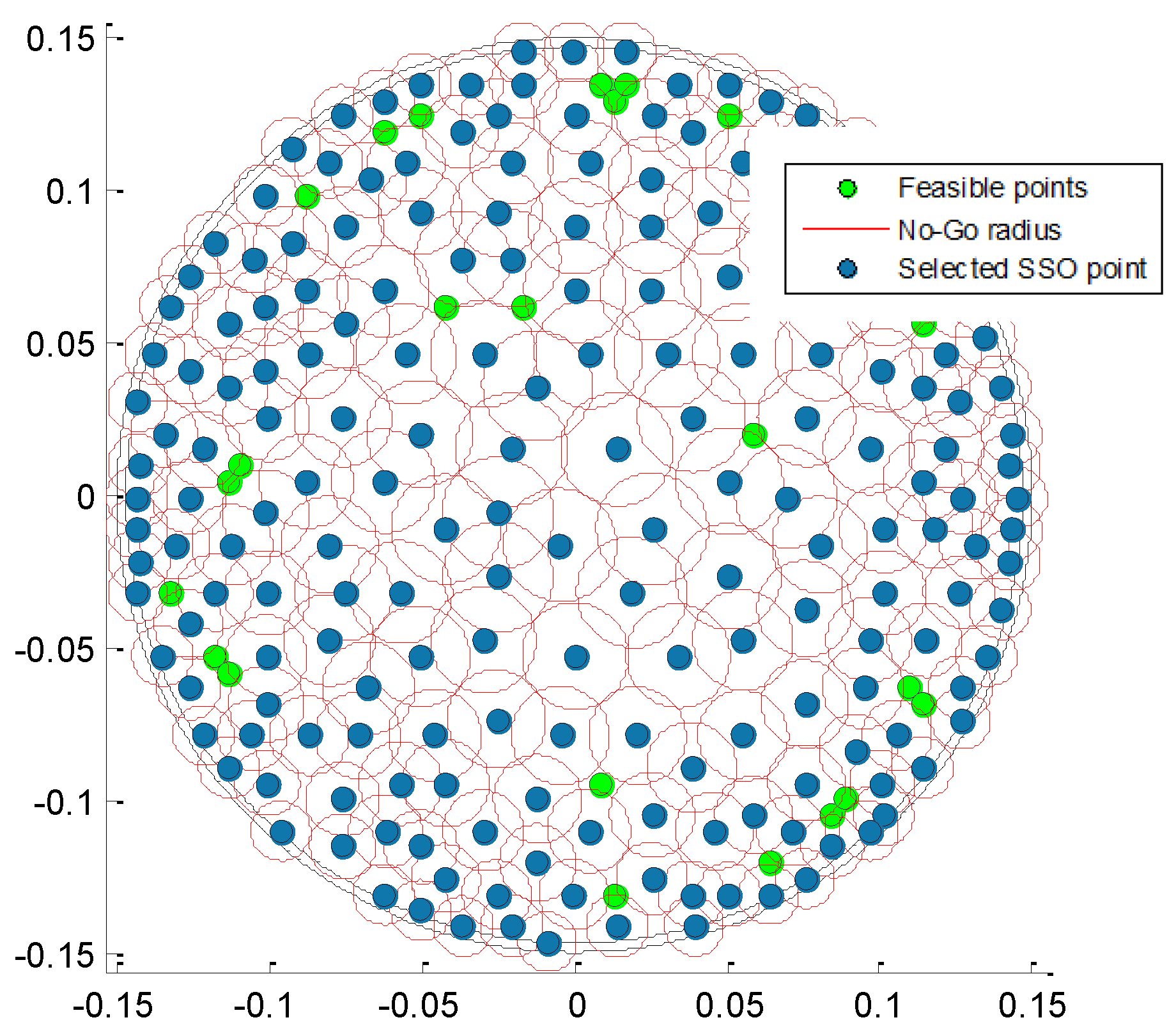
In
Figure 7, a nice visualization of the progress of the above algorithm is presented. In green, we see the points that qualify as candidates at a specific iteration of the process while the points that are already part of the scheme are shown in blue. In this case, the
k nearest neighbors of the already selected points are disqualified, with
k depending on the iteration of the algorithm since we start with
and this is further reduced. Hence, the disqualified points are the ones belonging to the area that the red circles define. In a very careful look, we notice that the red circles in the center are larger than the circles on the edge of the wafer. This is because the points in the center of the wafer were selected at an earlier stage of the points on the edge. Hence, at that step of the process, the exclusion zone defined by the
k disqualified neighbors is bigger (for enforcing uniforming) but as the process continues, a large
k yields no available points. In that case,
k decreases as described above, and the circle of the exclusion zone becomes smaller.
In the end of the above process, we obtain a scheme containing 221 selected points, which are uniformly sampled and with spatial randomness ensured, which, most importantly, ends at the same time as a near D-optimal design.
3.2. Improving Solution with Genetic Algorithms (GAs)
In the previous part of our algorithm, we created an initial population of, in this case, 30 solutions. The strategy though that we followed can be considered “greedy” since we add to the schemes the point that contributes more to the D-optimality. A greedy algorithm makes locally optimal choices at each step with the hope of finding a global optimum, but it may not always lead to the best solution overall. It is important to strike a balance between the optimality criterion and practical considerations when designing an algorithm for a real-world problem. Hence, at this part of the algorithm, we propose genetic algorithms to balance out the greedy approach. In fact, one of the strengths of GAs is that they can help overcome local optima that might be encountered with a purely greedy approach.
In our problem, after ensuring the uniformity of the samples, we aim to find an optimal solution in terms of G-, D-, and A-optimality, which is a multi-objective optimization problem. Multi-objective optimization seeks to find solutions that produce the best values for one or more objectives, typically having a series of compromising options known as Pareto optimal solutions rather than a single optimal solution. In our case, we simplify the multi-objective problem as a single objective by aggregating multiple objectives into one using a weighted sum. Our use case allows for this simplification since the three different objectives are very similar, representing different metrics of the same goal. Thus, the cost function of our genetic algorithm is the compound criterion of G-, D-, and A-optimality, similar to the second step of the process.
The genetic algorithm draws its inspiration from the natural selection process. It is a population-based search algorithm that applies the survival of the fittest principle. The main components of the genetic algorithm are chromosome representation, selection, crossover, mutation, and fitness function computation. The genetic algorithm process involves the initialization of an n-chromosome population (
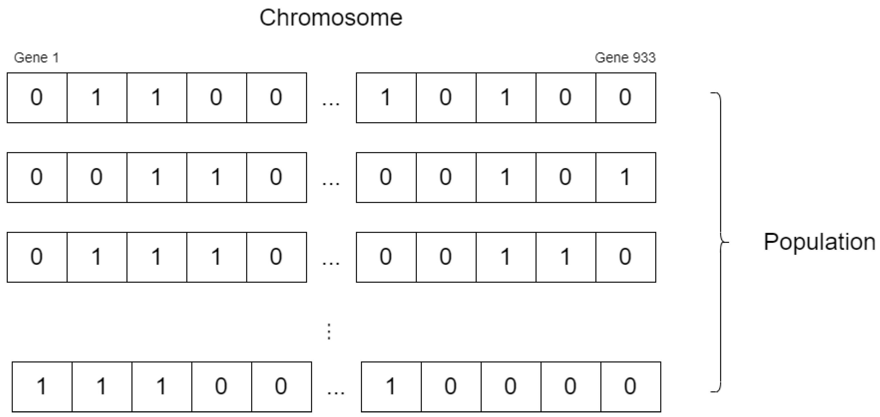
Y), which is usually randomly created, but in our proposed strategy, the initial population is created using a deterministic approach, except for the first two random points. This detail plays a significant role in the quality of the results and the robustness of the proposed algorithm. We propose a chromosome representation approach for optimizing sensor placement configurations where each chromosome represents a candidate sensor placement configuration and consists of a 1D binary array with a length of 933, as shown in
Figure 8. The elements in the array correspond to available points that can be selected for sensor placement. A value of 0 indicates that a specific point is not selected in the final scheme, while a value of 1 signifies its inclusion. This binary encoding allows the GA to explore the solution space and identify optimal sensor placement configurations.
Then, the fitness of each chromosome in
Y is calculated, and two chromosomes, designated
and
, are selected based on their compound criterion fitness values. The single-point crossover operator with the crossover probability (
) is applied to
and
to produce an offspring,
O. The offspring
O is then subjected to the uniform mutation operator with mutation probability (
) to create
.
is then added to the new population, and this process is repeated until the new population is complete. Mutations are performed in pairs. If a gene assumes a value of 1 (which means that it is selected) and it is mutated to a value of 0 (not selected), then another one of the genes, having a value of 0, is picked at random and its value becomes 1. Likewise for genes assuming value 0. Thus, the number of active points is maintained after each mutation occurs. GA dynamically modifies the search process using the probabilities of crossover and mutation to arrive at the best solution. GA can change the encoded genes, and it can evaluate multiple individuals to generate multiple ideal results, giving it a higher ability for global search. The core part of the GA is the fitness function. In our solution, we propose a compound criterion of G-, D-, and A-optimality instead of using only one type of optimality. Using a compound criterion that combines multiple types of optimality (such as D-, G-, and A-optimality) in a GA fitness function can be beneficial for several reasons. Firstly, using a single type of optimality can result in the GA getting trapped in a local optima. Local optima are solutions that appear to be optimal in the immediate vicinity but are not the globally optimal solution. By using a compound criterion that considers multiple types of optimality, the GA can search for a solution that is not only locally optimal but also globally optimal. Secondly, a compound criterion can help balance different types of optimality. For example, a solution that is highly optimized for D-optimality may not be optimized for G-optimality or A-optimality. By combining these different types of optimality, the GA can search for a solution that is optimized across all dimensions. Finally, a compound criterion can help ensure that the GA converges to a solution that is practical and usable in real-world situations. For example, a solution that is optimized for D-optimality may not be feasible to implement due to other practical considerations such as cost or manufacturing constraints. By combining different types of optimality, the GA can search for a solution that is both optimal and feasible to implement. More specifically, we define the fitness function as:
In this scenario, the multi-objective optimization problem requires that all objectives are equally taken into account while giving slightly more weight to G-optimality. This is achieved by assigning a weight of 0.4 to G-optimality, and weights of 0.3 to both D-optimality and A-optimality, in the compound criterion used for evaluating the fitness of the solutions generated by the GA. By giving more weight to G-optimality, we can bias the optimization process towards generating solutions that have a good overall fit to the data, while still taking into account the other objectives. This can help avoid the problem of getting trapped in the local optima, since the GA will be better able to explore the search space and find better solutions that are not necessarily optimal in any one objective but that are good overall. Furthermore, the use of multiple objectives in the fitness function can help generate more diverse and robust solutions, since this allows the GA to explore a larger space of potential solutions. This can help avoid over-fitting to the training data and improve the generalization performance of the model. In the given fitness function, we have a constraint that the solution should not have more than 221 elements. If a solution violates this constraint, we need to penalize it to discourage the GA algorithm from selecting it. Penalizing a solution means assigning a high cost to it, which in turn lowers its fitness value. In our case for ensuring that we have 221 points in the final solution, the fitness function first checks whether the sum of the elements in the solution is equal to 221. The Kronecker delta function is used to count the occurrences of the value of 1 in the binary array representing the solution. For each element in the array, if it is equal to 1, the Kronecker delta function evaluates to 1, indicating the presence of one. The count of such occurrences is then summed up using the sigma notation . If it is not, we assign a penalty to the solution by adding a very high value (100,000) to the sum of the elements in the solution. This will make the fitness value of the solution extremely high, which means it will have a very low chance of being selected by the GA algorithm, since we are solving a minimization problem. Finally, the GA will have the following settings:
- 1.
The initial population consists of 30 solutions, which were created using the sensor mark selection based on the Poisson-disc and D-optimality techniques described above;
- 2.
The size of the population is set to 100, meaning that there will be 100 solutions in each generation;
- 3.
The algorithm will run for 50 generations;
- 4.
The probability of crossover is set to 0.6, meaning that there is a 60% chance that the two parent solutions will be combined to produce a new offspring solution in each crossover event;
- 5.
The probability of mutation is set to 0.05, meaning that there is a 5% chance that each gene in a solution will be mutated during a mutation event;
- 6.
Elitism is enabled, which means that the best solution from the previous generation will always be included in the next generation;
- 7.
The fitness function will be maximized, meaning that the algorithm will try to find solutions with the highest possible fitness value.
In our case, the genetic algorithm significantly improves the solution in terms of G-, D- and A-optimality, as demonstrated in
Section 4.
4. Experimental Results
The newly proposed OED strategy is evaluated using G-, D-, and A-optimality, the Fisher-based criteria describing the different flavors of dispersion, and in accordance, the amount of information that a certain solution can provide. As mentioned above, the uniformity of the selected marks on the wafer is also a requirement, but since it has already been taken into account during the creation of the search space for our solution and consecutively ensured from the Poisson-disc sampling part of the algorithm, it is not needed to be included in the evaluation criteria.
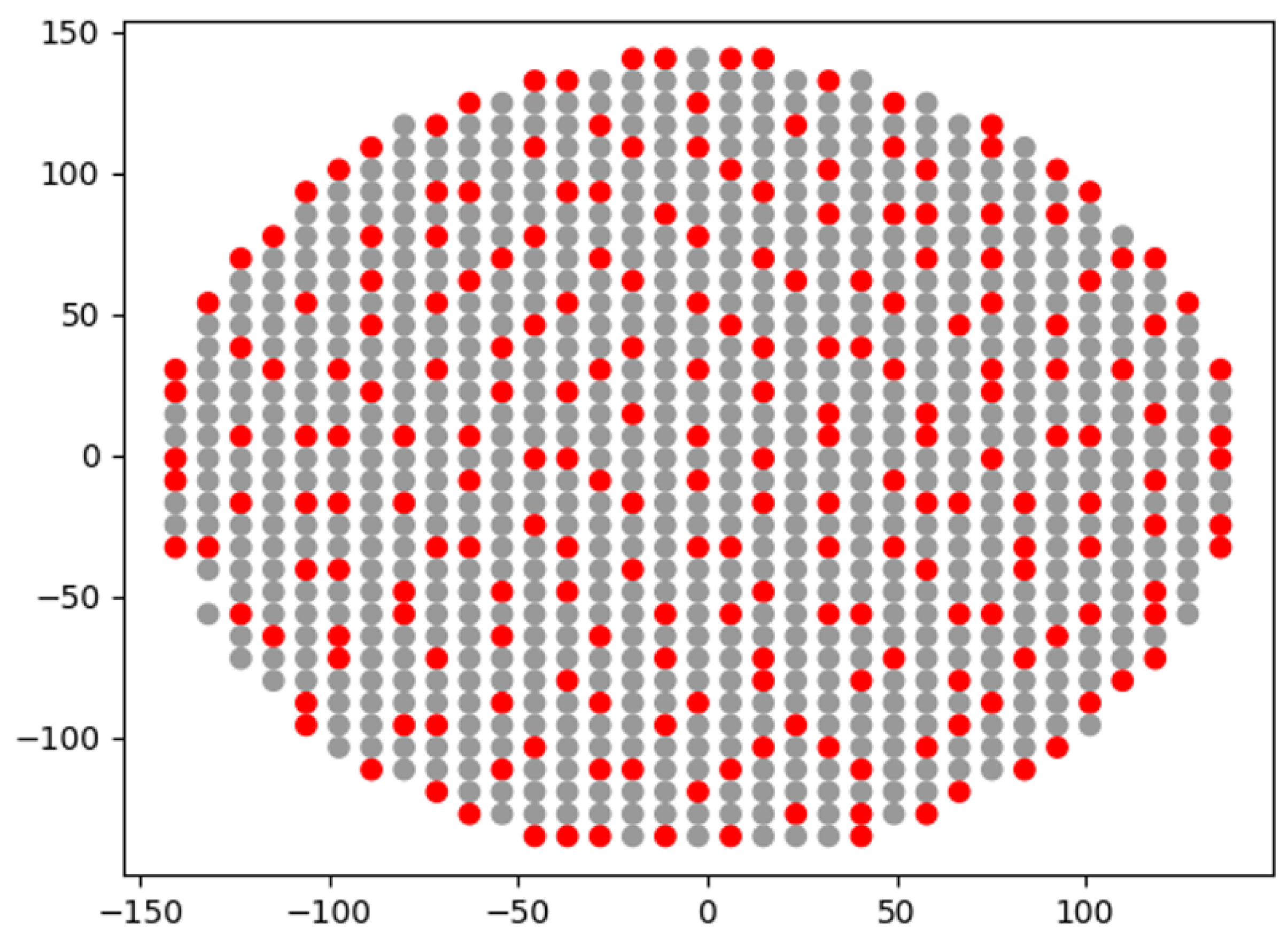
In
Figure 9, the selected marks on the wafer surface are represented. The points that were finally selected to participate in the sampling scheme are denoted in red, while the points that were not are shown in gray. All together, these form the candidate points. From
Figure 9 we can safely conclude that the solution satisfies the uniformity requirement.
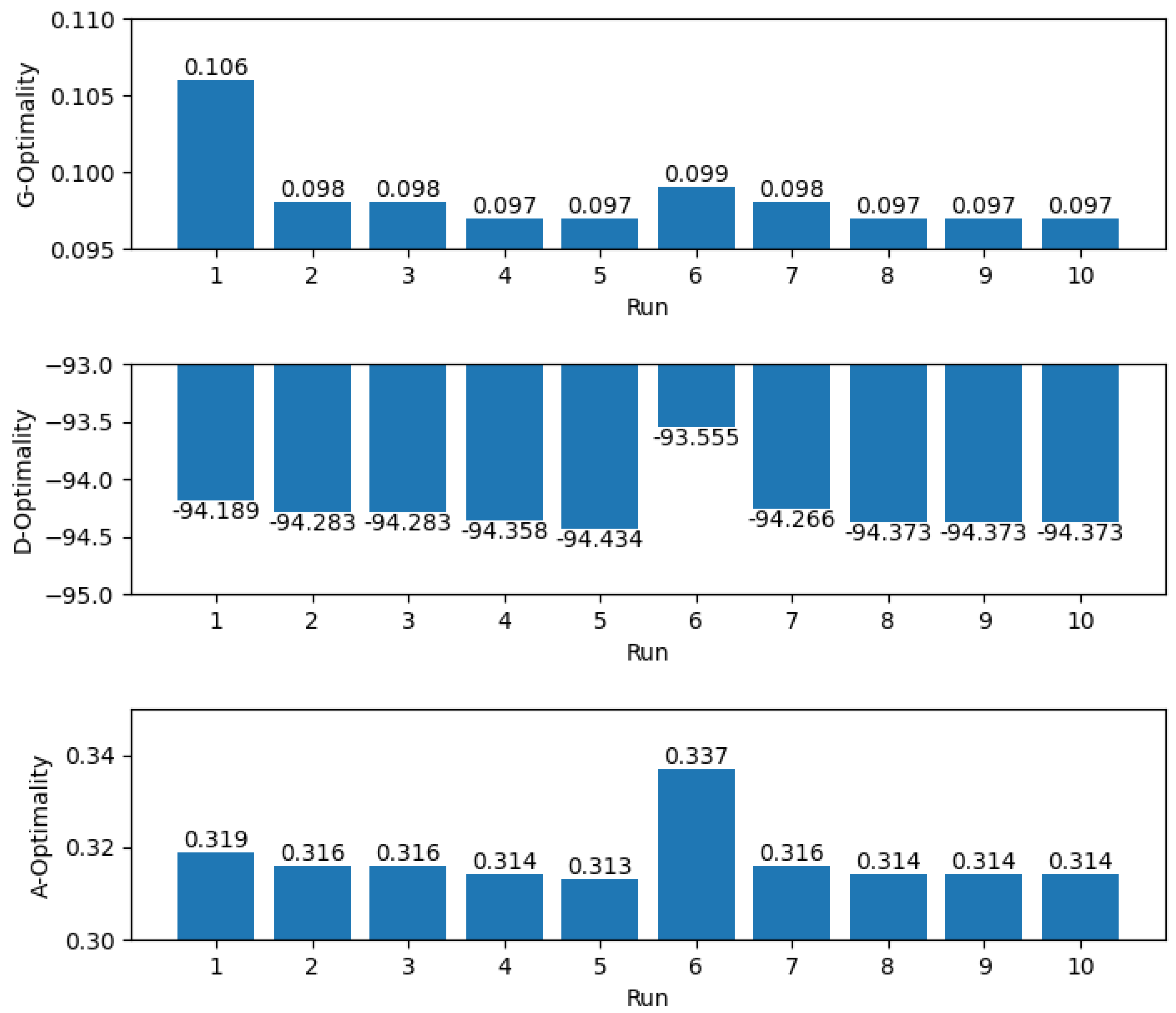
In
Table 1, the results of the 10 different runs of our algorithm are presented. From this table, we can draw two important conclusions. On the one hand, obviously the results are of high quality. As one can see, G-optimality is in the worst case 0.106, while we can see that for the rest of the runs, it is between 0.099 and 0.097.
From the theory of optimal experimental design, it is known that any G-optimality score below 1.00 is considered a satisfactory result. The proposed algorithm of Magklaras et al. [
15] achieves a G-optimality of around 0.261 which is considered a very good result. This result is achieved without improving the solution. In our proposed strategy, not only did we achieve a 10 times better result than the expected, but the result was also 3 times better than that obtained by Magklaras et al. [
15] by exploiting GAs in the final step. So, compared to previous work on the same problem, we can safely conclude for the success and superiority of our proposed solution.
Similarly, D-optimality also achieves high scores. In
Figure 10, we see that there is an outlier of −93.555 and the rest of the run achieves a score that is less than −94.1. A-optimality is also around 0.31 with only one outlier at 0.337, as shown in
Figure 10.
The second important conclusion is that, as can be seen from
Table 1, all G-, D-, and A-optimality scores are not only precise but also accurate. The dispersion of all three metrics is low and it seems that the genetic algorithm converges around certain values. For G-optimality at 0.097, for D-optimality around −94.373, and for A-optimality around 0.314. The observation that the genetic algorithm (GA) converges to the same solution over multiple independent runs is an important finding. GA is a stochastic optimization algorithm, meaning that it uses randomization to explore the search space. As a result, the algorithm may find different solutions each time it is run, and the convergence to the same solution over multiple runs is not guaranteed. However, the fact that the GA converges to the same solution over multiple independent runs suggests that the proposed solution is robust, meaning that it is less sensitive to variations in the randomization used by the algorithm. The robustness of the solution is an important property because it indicates that the solution is more likely to be useful in practice. In real-world applications, the inputs and conditions can vary, and a robust solution is more likely to perform well across different scenarios. Additionally, the observation that the GA converges to the same solution over multiple runs increases the confidence in the optimality of the proposed solution, as it suggests that the solution is not just a lucky outcome of the randomization used by the algorithm.
Finally, we have to mention that our algorithm runs in a simple workstation (CPU Intel i5) in only 10 min and using Python programming language. We understand that, in a non-prototyping but in a real-life industry scenario, this performance can be drastically improved. However, this is not necessary since this is an offline process and there is no strict requirement in terms of execution time.


 ,
, 


