Article

Federated Edge Intelligence and Edge Caching Mechanisms †

by
Aristeidis Karras
1,*,
Christos Karras
1,*,
Konstantinos C. Giotopoulos
2,
Dimitrios Tsolis
3,
Konstantinos Oikonomou
4 and
Spyros Sioutas
1
1
Computer Engineering and Informatics Department, University of Patras, 26504 Patras, Greece
2
Department of Management Science and Technology, University of Patras, 26334 Patras, Greece
3
Department of History and Archaeology, University of Patras, 26504 Patras, Greece
4
Department of Informatics, Ionian University, 49100 Kerkira, Greece
*
Authors to whom correspondence should be addressed.
This paper is an extended version of our paper published in the 7th IEEE South-East Europe Design Automation, Computer Engineering, Computer Networks and Social Media Conference (SEEDA-CECNSM), Ioannina, Greece, 23–25 September 2022.
Information 2023, 14(7), 414; https://doi.org/10.3390/info14070414
Submission received: 14 April 2023 / Revised: 11 June 2023 / Accepted: 22 June 2023 / Published: 18 July 2023

Abstract

:
Federated learning (FL) has emerged as a promising technique for preserving user privacy and ensuring data security in distributed machine learning contexts, particularly in edge intelligence and edge caching applications. Recognizing the prevalent challenges of imbalanced and noisy data impacting scalability and resilience, our study introduces two innovative algorithms crafted for FL within a peer-to-peer framework. These algorithms aim to enhance performance, especially in decentralized and resource-limited settings. Furthermore, we propose a client-balancing Dirichlet sampling algorithm with probabilistic guarantees to mitigate oversampling issues, optimizing data distribution among clients to achieve more accurate and reliable model training. Within the specifics of our study, we employed 10, 20, and 40 Raspberry Pi devices as clients in a practical FL scenario, simulating real-world conditions. The well-known FedAvg algorithm was implemented, enabling multi-epoch client training before weight integration. Additionally, we examined the influence of real-world dataset noise, culminating in a performance analysis that underscores how our novel methods and research significantly advance robust and efficient FL techniques, thereby enhancing the overall effectiveness of decentralized machine learning applications, including edge intelligence and edge caching.

1. Introduction

The swift progression of artificial intelligence (AI) has led to the proliferation of autonomous systems aimed at improving human quality of life. However, concerns regarding personal privacy have arisen [1,2]. To address these concerns, major technology companies such as Google and Apple have adopted federated learning (FL) approaches in widely-used applications such as Siri, Google Chrome, and Gboard. FL is a distributed machine learning method that enables training on decentralized data repositories located on devices such as smartphones [3]. The local updates are merged by a central server, addressing data privacy, ownership, and localization issues [4]. The merging process involves the FedAvg algorithm, which iteratively averages weights from models trained by each client for multiple local epochs [4]. To enhance convergence speed and resilience, additional aggregation methods such as FedDF, an ensemble distillation algorithm, have been developed [5].
The integration of federated learning (FL) in various applications represents a significant paradigm shift in machine learning, offering new opportunities for secure and collaborative data analysis [6,7,8]. FL’s decentralized approach, with data stored on local devices, mitigates risks associated with centralized storage and processing, ensuring enhanced data protection and compliance with privacy regulations. Moreover, FL enables the development of contextually relevant and personalized models, improving the effectiveness of AI-driven solutions. However, FL adoption also introduces challenges, such as the need for communication-efficient techniques and addressing biases in non-iid data. Ongoing research efforts are essential to address these concerns and promote the responsible and ethical deployment of AI technologies in an interconnected world.
Edge intelligence combines the benefits of edge computing and artificial intelligence [9,10,11], aiming to provide efficient data processing and analysis on devices at the network’s edge, such as IoT devices [12] and smartphones [13,14]. Blockchain-enabled edge intelligence has emerged as a promising approach to secure IoT applications by enhancing transparency, traceability, and data integrity [15]. In the context of smart grids, edge intelligence can offer advanced architectures, offloading models, and cybersecurity measures to address challenges related to energy management and distribution [16]. Moreover, in precision agriculture, unmanned aerial vehicles leverage remote sensing and edge intelligence to improve crop monitoring and optimize agricultural processes [17]. Lastly, a systematic review of TinyML, highlighting its potential impact and challenges in the field of edge computing, is presented in [18].
Communication-efficient federated learning has been proposed to enhance wireless edge intelligence in the IoT, addressing the challenges associated with data privacy, latency, and bandwidth consumption [19,20,21,22]. The integration of deep learning and computational intelligence in edge-enabled industrial IoT can significantly improve data-driven decision-making and automation [23]. Deep reinforcement learning, when combined with federated learning, can facilitate intelligent resource allocation in mobile edge computing, leading to enhanced performance [24]. Federated learning, as a cornerstone of edge computing, has been extensively studied, with researchers exploring its various aspects and potential applications in diverse domains [25].
The ongoing challenge of selecting between asynchronous and synchronous training algorithms within the framework of federated learning (FL) has been extensively researched in the field of deep learning. While asynchronous training has been widely utilized in previous studies, such as the work by Dean [26], recent research has shown a consistent shift towards synchronous large batch training, even in data centers. The Federated Averaging (FedAvg) algorithm follows a similar approach, emphasizing the need for synchronization. Furthermore, in order to enhance privacy assurances in FL, techniques such as differential privacy [27] and secure aggregation [28] require a level of synchronization on a fixed set of devices, allowing the server-side of the algorithm to process only a straightforward aggregate of updates from multiple users.
Previous research has assessed the performance of federated learning (FL) in relation to algorithmic selections, frequently through the simulation of the federation on centralized computation clusters [5]. The primary objective of our present study was to capture the distinctive hardware configurations that are characteristic of federated learning (FL) use cases, such as smartphones, where data are distributed across numerous edge devices with limited computational capabilities. To achieve this, we conducted local training of a convolutional neural network (CNN) on a set of 40 Raspberry Pi devices, with the CIFAR-10 dataset distributed among them. Subsequently, we leveraged techniques such as FedAvg, FedDF, and other aggregation methods to combine these locally trained models.
The overarching aim of our research was to thoroughly investigate the impact of FedAvg hyperparameters—specifically, the number of clients per communication round and local epochs—on the duration of convergence. We also aimed to assess the resilience of the aggregation process in the presence of imbalanced and noisy data and to identify any performance trade-offs that may arise in the context of physical hardware. The analysis we present provides valuable insights into the behavior and efficacy of FL algorithms in real-world hardware configurations, particularly in light of the unique challenges posed by periphery devices with limited computational resources. Additionally, we investigated conventional FL enhancements using four distinct methods: utilization of a peer-to-peer (P2P) network with client-processed weights; implementation of a P2P federated learning strategy; formulation of a Federated Averaging with Momentum scheme; and construction of a Federated Averaging with Adaptive Learning Rates scheme. This manuscript serves as an expanded version of our conference paper [29], which provided a preliminary exploration of the subject matter.
This work presents significant contributions in the field of federated learning, including novel algorithms and techniques that enhance performance, convergence speed, and efficiency. These contributions address important challenges such as optimizing label distribution, handling heterogeneous data distributions, optimizing parameters, and integrating edge caching strategies.
  • Enhanced Client-Balancing Dirichlet Sampling (ECBDS) (Algorithm 1): We proposed ECBDS, a novel sampling technique that optimizes label distribution in federated learning scenarios. By improving the representation of labels across clients, ECBDS enhances the overall performance and generalization capabilities of federated learning models. This technique is among the novelties of our work, as other state-of-the-art methods do not perform a similar data distribution measure;
  • A Client-Side Method for Peer to Peer Federated Learning is presented in Algorithm 2 along with a Peer to Peer Federated Learning Approach which shown in Algorithm 3.
  • FedAM (Algorithm 4), for Raspberry Pi Devices: We introduced the FedAM algorithm, specifically tailored and tested for resource-constrained Raspberry Pi devices. This algorithm accelerates convergence and mitigates the impact of noisy gradients in federated learning settings. FedAM offers a practical solution to improve model performance on edge devices, enabling efficient and robust federated learning deployments;
  • FedAALR (Algorithm 5), for Heterogeneous Data Distributions: Our proposed FedAALR algorithm addresses the challenge of heterogeneous data distributions in federated learning. By adaptively adjusting learning rates for individual clients, FedAALR enhances convergence speed and model performance. This contribution ensures that federated learning systems can effectively handle diverse and unevenly distributed data sources;
  • Parameter Optimization in FedAM: We focused on parameter optimizations specifically for the FedAM algorithm. By fine-tuning key parameters, we achieved improved convergence speed and stability in federated learning processes. This contribution enables practitioners to maximize the effectiveness and efficiency of FedAM-based federated learning systems;
  • Integration of Edge Caching Techniques: We enhanced the FedAALR algorithm by incorporating edge caching techniques. By strategically caching frequently accessed data at the network edge, we reduced communication costs and latency, making the algorithm more efficient. This integration of edge caching contributes to the scalability and practicality of federated learning deployments in resource-constrained environments.
The subsequent sections of this article are organized in a structured manner to provide a comprehensive overview of the research conducted. After a brief summary of the current research on federated learning, Section 2 then delves into a discussion of several publications that are connected to the topic. In Section 3, the methodology employed in this study is described in detail, both at a theoretical and application level, providing a clear understanding of the approach. The experimental results and their findings are presented in Section 4, accompanied by a comprehensive analysis and optimization in Section 5. In Section 6, a detailed discussion of the results is provided, critically analyzing the implications and limitations of the study. Finally, the conclusions drawn from the research and the future directions of this work are outlined in Section 7, summarizing the key findings and proposing avenues for further research in this field. The organized structure of this article aims to facilitate a systematic and in-depth understanding of the research objectives, methodology, results, and implications for the reader.

2. Literature Review

2.1. Evolution of Federated Learning

Federated learning (FL) is a privacy-preserving approach where multiple organizations collaborate to train a machine learning model [3]. Data privacy regulations, such as GDPR, prohibit the use of data without user consent. FL overcomes this challenge by allowing each organization to develop a task model using its local data while keeping the data private. Through encryption techniques, model parameters are exchanged between clients and a central server to create a global model without violating privacy protection laws. FL ensures privacy while enabling collaborative model training in a distributed manner.

2.2. Horizontal Federated Learning

Horizontal federated learning (HFL) is a FL subcategory that is applicable when using features that significantly overlap across two datasets, but the users themselves do not. HFL involves horizontally partitioning datasets (across user attributes) and eliminating the data segments with matching user features but different users for training. Consequently, different rows of data with similar features can be used to increase the sample size of users.
Suppose we consider two providers that offer identical services but operate in separate locations, catering to regional users with minimal overlap. Despite the similarities in their services, the user features of these providers are likely to be comparable as well. One approach to enhance the accuracy of the model and increase the total training samples is by employing horizontal federated learning (HFL) [30,31,32]. In HFL, participants can compute and submit local components to a central server, which then merges them into a global model. However, this process of processing and transferring components may pose a risk of revealing user information, raising concerns about privacy and security. To mitigate this issue, several common solutions have been proposed, including the use of homomorphic encryption schemes [33], differential privacy methods [27], and secure aggregation frameworks [34]. These techniques can ensure the security of gradient exchange in HFL, safeguarding the privacy of user data while facilitating effective collaboration and model improvement among providers.
In 2016, Google introduced an FL modeling methodology for Android phones [28], permitting users to modify model parameters locally before transferring them to the cloud. This approach allows data proprietors possessing congruent feature dimensions to construct an FL model. The framework encompasses various fundamental implementations of horizontal federated learning (HFL), which incorporate techniques such as differential privacy [27] and secure aggregation. For instance, BlockFL, a notable HFL system proposed in [35], utilizes a blockchain network to facilitate updates of local learning models on devices while an FL-based blockchain solution is presented in [36]. In another study [37], the authors introduced MOCHA, an FL technique that addresses security challenges in multi-task settings, enabling multiple sites to collaborate on tasks while preserving privacy and security.
An alternative approach, known as multi-task federated learning, aims to reduce communication expenses and enhance fault tolerance compared to conventional distributed multi-task learning methodologies. For example, in [4], it was shown that HFL enables privacy-secure, collaborative learning by letting clients develop and share local models without uploading sensitive data. This embodies ongoing efforts to address distributed machine learning challenges.

2.3. Vertical Federated Learning

Vertical federated learning (VFL) is a promising solution for scenarios with minimal overlap in user features across datasets but significant overlap in users. By vertically partitioning datasets along the user/feature dimension, VFL expands the training data by representing the same user in multiple columns.
This approach improves the performance of federated models while preserving data privacy and security.
VFL has been successfully applied to various machine learning models, such as logistic regression, tree structure models, and neural networks. Ongoing research in VFL focuses on developing advanced techniques and algorithms to enhance efficiency, scalability, and privacy guarantees in real-world applications. By addressing challenges associated with disparate user features, VFL advances federated learning as a robust and privacy-preserving approach for collaborative machine learning in interconnected environments, such as financial institutions and e-commerce brands operating in the same geographical location.
In recent years, vertical data partitioning has emerged as a prominent technique for federated learning, where data from multiple sources are collaboratively used for model training without sharing raw data. This approach poses unique challenges due to the distribution of data along the user/feature dimension, which requires novel solutions to ensure effective model training while preserving data privacy and security. A plethora of machine learning techniques have been developed to address the unique challenges associated with vertical data partitioning, including classification [38], statistical analysis [39], gradient descent [40], privacy-based linear regression [41], and privacy-focused data mining methods [42]. Notably, recent research has proposed innovative approaches to tackle these challenges within the context of vertical federated learning (VFL).
For instance, Cheng et al. [43] proposed a VFL system called SecureBoost, where all participants contribute their user features for joint training, with the goal of improving decision-making accuracy. Remarkably, this training scheme is designed to be lossless, ensuring the preservation of privacy and data integrity during the federated learning process. Furthermore, Hardy et al. [44] presented a privacy-preserving logistic regression model based on VFL. This approach leverages techniques such as parallelizing objects for analysis and distributed logistic regression with supplementary homomorphic encryption [45], which enhances the protection of data privacy and classifier accuracy.
These examples highlight the growing interest in addressing challenges related to vertical data partitioning in federated learning. By developing innovative techniques, researchers aim to overcome these challenges and advance privacy-preserving solutions for real-world applications. Ongoing research in this field focuses on further enhancing the efficiency, scalability, and security of vertical federated learning and related techniques. The ultimate goal is to enable effective and secure federated learning across diverse domains.

2.4. Incorporating Edge Intelligence with Federated Learning

The integration of edge intelligence [46,47] and fully distributed federated learning marks a significant development in machine learning research. This integration leverages the capabilities of edge devices such as smartphones, IoT devices, and smart sensors, creating an efficient, privacy-preserving machine learning system focused on local data processing and analysis.
The combination of these two complementary technologies forms a unique, distributed machine learning system. It enables real-time local data processing and analysis without depending on cloud-based services. The approach taps into decentralized data sources to enhance the accuracy and robustness of machine learning models, reducing the latency and bandwidth requirements of machine learning applications. Simultaneously, it ensures improved data privacy and security.
This strategy’s novelty lies in the marriage of edge intelligence with fully distributed federated learning. It highlights the potential growth and expansion in the machine learning field, as machine learning algorithms are implemented on peripheral devices. Despite the lack of dependence on cloud services, the system manages to perform real-time local data processing and analysis. The distributed nature of federated learning enhances the precision and robustness of ML models by utilizing decentralized data sources.
Significant effects of this strategy are observed in real-world applications such as autonomous vehicles, healthcare monitoring, and industrial automation. The deployment of machine learning algorithms on peripheral devices improves their performance and efficiency, underlining the strategy’s broad implications for such applications.
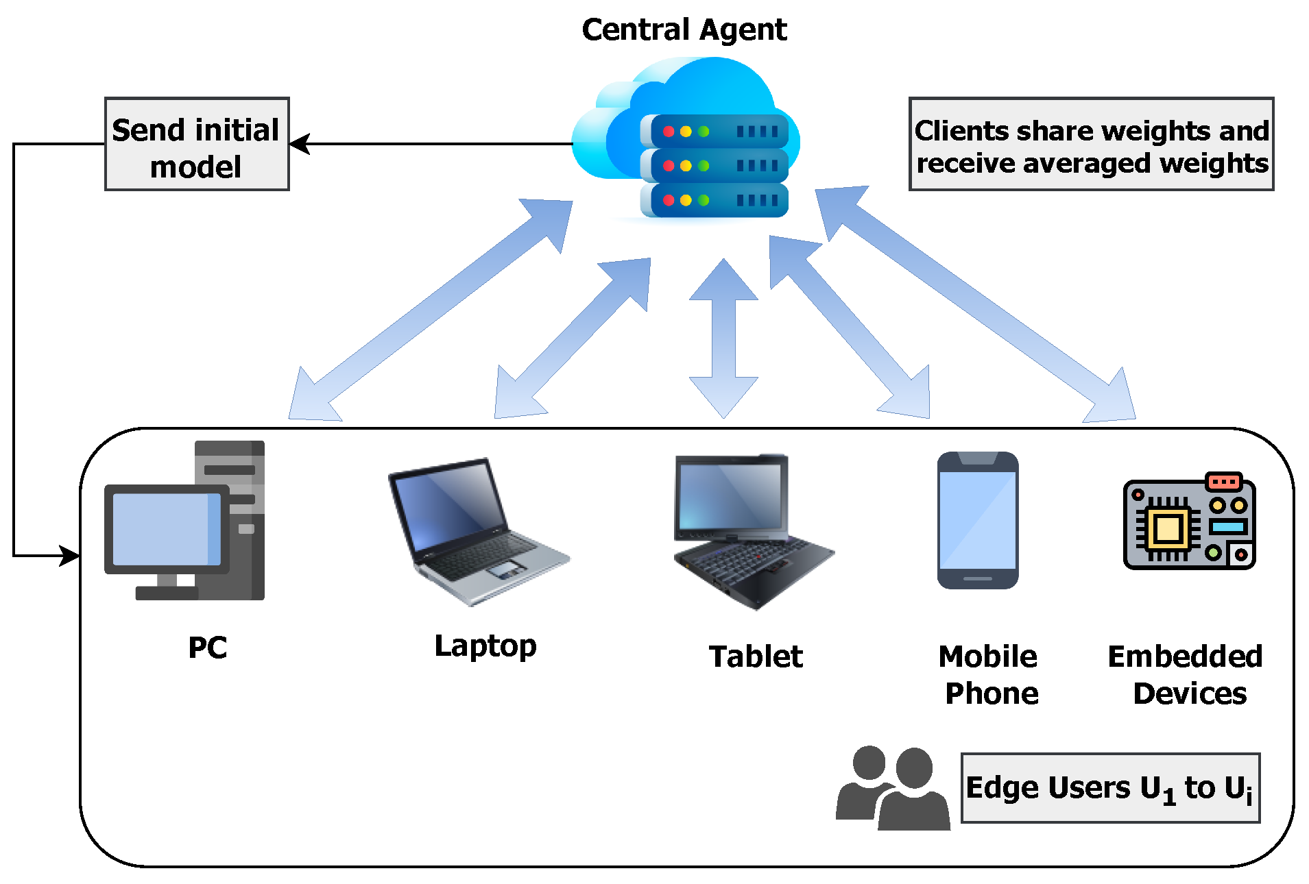
The integration of edge intelligence with fully distributed federated learning is a viable path for advancing machine learning technology across different sectors. By bringing together the benefits of both learning types, it paves the way for further research and development. This might lead to the creation of highly efficient, accurate, decentralized, and secure machine learning systems with wide-ranging applications. The architecture of such a system, integrating Distributed Federated Learning with Edge Intelligence, is depicted in Figure 1. Lastly, in Table 1, the available methods in federated learning are presented along with their advantages and limitations.

3. Proposed Methodlogy

3.1. Understanding Federated Learning Techniques

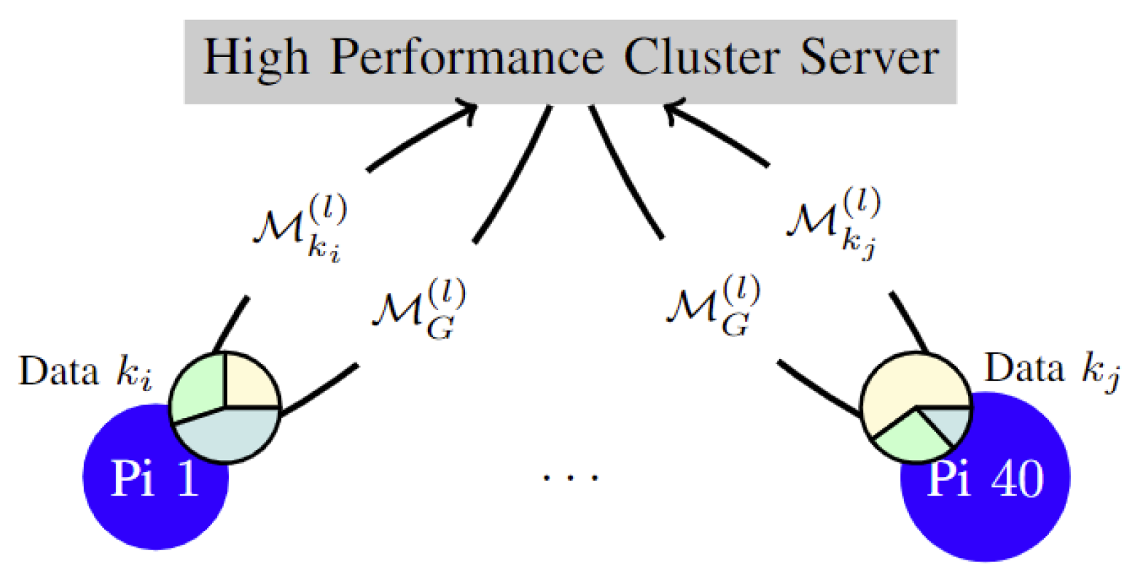
In this section, we explore the concept of federated learning and how it is implemented. Federated learning (FL) is a process that involves the collaboration of K clients, each of whom holds a unique portion of a larger training dataset with size n k . A global model, represented as M G , is hosted on a central server. Over the course of L rounds, known as communication rounds, S K clients are selected using a Dirichlet sampling method. Each of the chosen clients is provided with a local copy of the global model M G . The architecture of federated learning is further illustrated in Figure 2. More information about the notation and symbols used in the article is given in Appendix A.1 while the hardware setup illustration is given in Appendix A.2.
The clients perform E local epochs of learning before sending their updated local models M k back to the central server. In the original FedAvg algorithm, the server combines the S received models by averaging their weights, consequently generating an updated global model for the next communication round. This process aims to minimize an implicit objective function f with respect to the model weights w, given a loss function :
f ( w ) = k = 1 K n k n total F k ( w ) , F k ( w ) = 1 n k i = 1 n k ( x i , y i ; w ) ,
Here, F k ( w ) represents the objective function for the k-th client [4].
An alternative aggregation method, the FedDF algorithm, is incorporated in this study. This technique replaces the weight averaging approach of FedAvg with ensemble distillation for fusing models using an unlabeled dataset similar to the training datasets. Utilizing hyperparameters comparable to those in [5], the global model M G ( l + 1 ) is generated by distilling the S local models M k i ( l ) through 10 4 batch updates against a Kulback–Leibler (KL) divergence criterion. A batch size of 128 and a learning rate of 10 3 are employed. Adam optimization with cosine annealing is applied in this process. Early stopping is incorporated by calculating the KL divergence against an unlabeled validation set every 10 3 updates and stopping if the evaluation loss fails to decrease. Section 3.8 provides a comprehensive explanation of the KL divergence criterion.

3.2. Embedded Systems

The technical dimension of this investigation, as depicted in Figure 3, encompasses two primary elements: a centralized high-performance computing (HPC) cluster and an array of 10 Raspberry Pi 4 units, each outfitted with 4 GB of RAM and a 1.5 GHz quad-core processor. It is important to note that the Raspberry Pi systems are linked to a distinct network, separate from that of the HPC, in order to simulate a more realistic communication environment.
A vital function of the HPC server is to aggregate the locally trained models generated by each individual device and subsequently assess the derived global model M G .
Each Raspberry Pi houses a Flask server that manages the model exchange, local training execution, and active memory usage monitoring—a crucial factor when operating in resource-limited hardware settings. Additionally, the server offers a pathway for transmitting requests, enabling vital over-the-air updates.
The Raspberry Pi setup can accommodate experiments with K > 10 , indicating that it can support over 10 clients and, as a result, dataset partitions with a restriction of no more than 10 clients sampled per round ( S 10 ). This is achieved by storing all K client datasets on every device, and during each communication round l, allocating each of the S sampled client datasets to a Raspberry Pi.
The Raspberry Pi devices connect to a switch, which in turn is linked to the router via a cable. When the switch is deactivated, the devices establish a connection through Wi-Fi, allowing for the evaluation of communication overhead in two distinct situations: the relatively fast Ethernet and the comparatively slow Wi-Fi. Specifically, the utilized network has a bandwidth of 100/100 Mbit/s, with Ethernet taking advantage of the full capacity and Wi-Fi using only around 10% (10/10 Mbit/s). As shown in Figure 3, each client corresponds to a dataset partition k 1 k S , with Raspberry Pi 1 training a model as client k i , and Raspberry Pi 40 as k j .

3.3. Problem Formulation and Dataset

To carry out the federated learning scenario mentioned previously, we used the CIFAR-10 computer vision (CV) dataset. This dataset consists of 32 × 32 images, which are classified into various object categories such as birds, cats, and airplanes. Due to memory limitations on the devices and to speed up training times, all images were converted to grayscale. The training dataset contained 5000 images for each of the 10 classes. For the model M , we chose a network consisting of two convolutional layers, followed by two linear layers, with more details available in the conference version of this work [29].
The dimensions of the model were purposefully kept small to fit within the memory limitations of Raspberry Pi devices. For optimization during the local epochs (E) on each device, the Adam optimizer was used, featuring a learning rate η that decays after each local epoch: η γ η , γ 1 .
In this section, imbalanced and noisy data were addressed. To simulate various degrees of imbalance, the Dirichlet distribution, Dir ( α ) , was employed:
  • The parameter vector α has a length equal to the number of labels—which was 10 in this case—and α i = α ;
  • Each sample π Dir ( α ) represents a probability distribution across labels, and α determines the corresponding distribution’s uniformity;
  • As α approaches 0, a single label dominates, whereas as α approaches infinity, π  becomes increasingly uniform. For α = 1 , every possible π has an equal probability of being selected;
  • For each client, π was sampled, making the label distribution Dirichlet for every client.
In order to maintain disjoint client datasets while optimizing the utilization of the entire dataset, a client-balancing Dirichlet sampling algorithm was devised, which is detailed in Section 3.4.
The client-balancing Dirichlet sampling algorithm takes into account the inherent imbalance present in real-world datasets, ensuring that the federated learning system remains robust and adaptable to such scenarios. By resolving the issues of imbalance and noise, we can provide a more thorough evaluation of the algorithms proposed in this study and gain a better understanding of their performance under realistic conditions.
Furthermore, the development of the client-balancing Dirichlet sampling algorithm allows for the effective distribution of data across clients, while simultaneously addressing the complexities introduced by imbalanced and noisy datasets. This approach enables the federated learning system to efficiently process data and improve overall performance, even when faced with diverse and challenging data characteristics.
In summary, the utilization of the Dirichlet distribution and the client-balancing Dirichlet sampling algorithm significantly contributes to the robustness and adaptability of the federated learning system in our study. These techniques enable the system to handle imbalanced and noisy data effectively, ensuring that the resulting models are capable of performing well in real-world scenarios where class balance cannot be guaranteed.

3.4. Enchanced Client-Balancing Dirichlet Sampling Algorithm

This section provides an expansion of the client-balancing Dirichlet sampling algorithm introduced in the concise version of this work [29]. Consider a dataset D with a total size of D , composed of l distinct labels, with each label containing D / l instances. The primary objective of the algorithm is to distribute the dataset across C clients, ensuring that the label distribution, π i , for each client i follows the same Dirichlet distribution, Dir ( α ) . All α j α ,   j = 1 l have identical values. For simplicity, the Dirichlet distribution was parameterized solely by α , denoted as Dir ( α ) .
These distributions are organized in a matrix P with dimensions C × l . The i-th row corresponds to π i . The i j -th element, P i j , signifies the fraction of label j on client i. The sum of the j-th column represents the relative usage of label j, scaled by the number of clients, C. To ensure equal usage of each label, every column should have a total of C / l . If the sum of any column surpasses this value, the corresponding labels are oversampled, necessitating the normalization of all P to equalize the largest column sum to C / l . This normalization procedure results in the omission of some data.
In the mapper stage of the algorithm at step 4, u values are exchanged, and step 9 executes all potential swaps. If no further swap is possible, step 19 terminates the process. Step 22 normalizes P based on the most-sampled label. To assess how closely P approaches the goal of equalizing each column sum, a measure, u, was employed. The smallest value of this measure should correspond to a P where every column totals to C / l , whereas higher values should be assigned to inferior P values. The L1 norm of the difference in column sums and C / l is adopted.
Let S represent the sum of the columns in matrix P :
S j = i = 1 C P i j , f o r j = 1 , , l .
The measure u can be defined as follows:
u = j = 1 l S j C l .
Then, based on Equation (3), we can express the C / l as in Equation (4):
u ( P ) = j = 1 l C l i = 1 C P i j
Equation (4) measures the absolute difference between the sum of each column in P and the target sum of C / l . To gain more insight, we can expand Equation (4) by adding a normalization term and an optional scaling factor as in Equation (5):
u ( P ) = j = 1 l C l i = 1 C P i j j = 1 l i = 1 C P i j · λ
where λ is a scaling factor. By default, λ = 1 , and the equation remains the same as before. However, by adjusting λ , we can emphasize or de-emphasize the importance of achieving equal column sums. A larger λ places more importance on the equal column sums, while a smaller λ diminishes their significance.
This client-balancing Dirichlet sampling algorithm enables the efficient distribution of datasets across clients while maintaining the desired label distribution in a federated learning setting. By implementing this algorithm, we can ensure that the federated learning system is able to handle imbalanced datasets and more closely mimic real-world scenarios.
Moreover, the algorithm addresses the challenges associated with the distribution of data in a federated learning context by employing a measure, u, to assess the closeness of the label distribution to the desired uniform distribution. This approach allows the federated learning system to adjust and enhance the data distribution with the aim of boosting the overall performance of the model.
Additionally, the normalization term in Equation (6) guarantees that the measure stays within a significant range:
i = 1 C P i j j = 1 l i = 1 C P i j
Let Q i j represent the normalized matrix element for the i-th client and the j-th label. The normalization term can be mathematically expressed as in Equation (7):
Q i j = P i j k = 1 C m = 1 l P k m ,
where P i j denotes the proportion of the j-th label on the i-th client before normalization and C and l represent the number of clients and distinct labels, respectively. The term in Equation (6) ensures that the measure u ( P ) is not affected by the overall scale of the matrix P . This makes the measure more robust and allows for comparisons across different scenarios, even if the scale of the label distribution varies. Similarly, standard deviation or the reciprocal of the entropy could be employed. The final aspect to consider before introducing the algorithm is that reordering π i makes it equally likely to be sampled from Dir ( α ) .
The α -values can be seen as a vector ff = ( α 1 , α 2 , , α l ) , which are essentially the parameters of the Dirichlet distribution. In the context of the federated learning, these parameters may represent the desired proportions of labels across clients.
The Dirichlet distribution itself, Dir ( α ) , can be expressed as in Equation (8):
Dir ( ff ) = 1 B ( ff ) i = 1 l x i α i 1 ,
where B ( ff ) is the multivariate Beta function, defined as in Equation (9):
B ( ff ) = i = 1 l Γ ( α i ) Γ i = 1 l α i ,
with Γ being the Gamma function.
The algorithm iterates and updates the α -values to gradually approach the desired distribution. It might be possible to use a method, such as gradient descent or another optimization method, to achieve this.
For example, if we denote the updated value of α at the t-th iteration as α ( t ) , and we apply an update rule based on the difference between the desired column sums C / l and the current column sums, we may write the update rule as in Equation (10):
α ( t + 1 ) = α ( t ) η S j C l ,
where η is the learning rate.
Finally, we can incorporate a stopping criterion based on u ( P ) , e.g., if the value of u changes less than a certain threshold, we could terminate the iterative process as in Equation (11):
Δ u = | u ( t + 1 ) ( P ) u ( t ) ( P ) | ,
i.e., if Δ u < ϵ (for a small positive ϵ ), stop the iterations.
Ultimately, the client-balancing Dirichlet sampling algorithm is an essential component of the federated learning system, enabling the efficient distribution of datasets across clients while maintaining the desired label distribution. By addressing the challenges associated with imbalanced data, the algorithm ensures that the federated learning system is able to more accurately represent real-world scenarios and deliver improved model performance.
The algorithm aims to iteratively change the ordering within each π i until the measure u ( P ) can no longer be minimized. The complete steps of this Enhanced Client-Balancing Dirichlet Sampling (CBDS) algorithm are presented in Algorithm 1. The original Client-Balancing Dirichlet Sampling algorithm is given in the short version of this work [29].
Algorithm 1 Enhanced Client-Balancing Dirichlet Sampling (ECBDS)
Require: Number of clients C, concentration parameter α
Ensure: Client-balanced distribution P
  1:
for i from 1 to C do
  2:
       P i Dir ( α )
  3:
end for
  4:
Calculate initial u ( P )
  5:
loop
  6:
       d Map()
  7:
      for i from 1 to C do
  8:
            for all  ( j 1 , j 2 ) ( 1 l ) × ( 1 l ) , j 1 j 2  do
  9:
     Swap P i j 1 and P i j 2
10:
      d [ ( i , j 1 , j 2 ) ] u ( P )
11:
     Swap P i j 1 and P i j 2 back
12:
            end for
13:
      end for
14:
      if  min ( d ) < u ( P )  then
15:
             i , j 1 , j 2 argmin ( d )
16:
            Swap P i j 1 and P i j 2
17:
            Update u ( P ) with the new value
18:
      else
19:
            Break
20:
      end if
21:
end loop
22:
Assign data points to clients based on the final P matrix
23:
π i = 1 C π i
24:
P P / max ( π )
25:
Return P as the final client-balanced distribution
The Enhanced Client-Balancing Dirichlet Sampling (ECBDS) algorithm is designed to create an optimized label distribution for federated learning scenarios. It starts by initializing the P matrix and calculating the initial u ( P ) measure. By performing swaps in the main loop and updating the u ( P ) measure with the new values obtained, the algorithm can effectively track progress during the optimization process.
Moreover, after the main loop, an additional step assigns data points to clients based on the final P matrix. This ensures that the distribution of data points among clients matches the optimized label distribution found by the algorithm. The algorithm then calculates the total label distribution, π , and normalizes the final P matrix by dividing it by the maximum value of π , making certain that all data points with the most sampled labels are used exactly once. The enhanced algorithm returns the final client-balanced distribution, P , which can be used for further processing or analysis.
The ECBDS algorithm performs well with a wide range of client and alpha values. For instance, when executed with C = 100 and α = 0.01 for 100 iterations, the average undersampling was less than 1%, with the largest undersampling being 3.3%. It is rare for any single label to be undersampled by more than 5%, demonstrating the strength of the algorithm, even for low values of α . The algorithm’s performance tends to improve with higher values of C and α , resulting in more evenly sampled labels.
The Enhanced Client-Balancing Dirichlet Sampling (ECBDS) algorithm exhibits a computational complexity of 𝒪 ( C ) for initializing the Dirichlet distributions for each client. The subsequent loop, exploring all possible swaps between labels of different clients, has a time complexity of 𝒪 ( C 2 · l 2 ) , where C represents the number of clients and l denotes the number of labels. Within the loop, the measure u ( P ) is calculated after each swap, with a time complexity of 𝒪 ( C · l ) . Finding the minimum value of u ( P ) using the argmin function also has a time complexity of 𝒪 ( C · l 2 ) . Assigning data points to clients based on the final P matrix can be accomplished in 𝒪 ( C · l ) time. Normalizing the P matrix and returning the final client-balanced distribution has a time complexity of 𝒪 ( C · l ) . The ECBDS algorithm converges to a locally optimal solution, as each swap either improves or maintains the measure u ( P ) . Thus, the algorithm achieves client-balanced distribution while exhibiting a computational complexity of 𝒪 ( C 2 · l 2 ) .

3.5. Adapting to Federated Learning in a Peer-to-Peer Context

This section discusses adapting federated learning to a peer-to-peer (P2P) context.

Peer-to-Peer Approach

In this section, we explore an extension to federated learning with a focus on a P2P scenario. Unlike the conventional FL setup where clients send their model weights and evaluation results to a central agent C that computes the average weights and returns the updated weights to the clients for the next learning round, in a P2P setting, the averaging process takes place locally on each client’s device without a central agent.
Each client U i in the set U sends its weights to all other clients. As a result, every client U i has access to the weights from all other clients in U, denoted as W others . Clients then carry out evaluations locally on their validation data using their model M i and models initialized with weights from the set W others . This allows each client to evaluate the relevance of other clients’ models to their data and take appropriate action based on the averaging methodology used. The evaluation results are used by each client to compute the averaged weights W avg , which are then employed in the next round of local learning. Since W avg is specific to each client, we denoted it as W i , avg .
We proposed two algorithms, Algorithms 2 and 3, to implement the P2P extension of standard FL. These algorithms have been enhanced from the conference version to provide a more comprehensive understanding:
  • Algorithm 2 details the client-side operations in P2P federated learning, which include computing the local average of the received set of weights, updating the model’s weights, evaluating the model, and training the model for a specified number of local epochs. The algorithm saves both pre-fit and post-fit evaluation results for further analysis;
  • Algorithm 3 illustrates the P2P federated learning approach, wherein devices exchange weights with one another, simulating P2P communication in a real-world scenario. The algorithm acts as a coordinator, collecting weights from each device and distributing the complete set of weights to all devices. The algorithm starts by sending the model M to all clients within U. Then, for each round of federated learning, it initiates the training of all clients, as shown in Algorithm 2.
Algorithm 2 Client-Side Operations in P2P Federated Learning
  1:
def  client(set_of_weights):
  2:
if set_of_weights != None: then
  3:
      updated_weights = compute_local_average(set_of_weights)
  4:
       M i .update_weights(updated_weights)
  5:
end if
  6:
initial_evaluation = device.evaluate_model ()
  7:
device.store_pre_fit_evaluation(initial_evaluation)
  8:
for e in  l o c a l e p o c h s :  do
  9:
       M i .train_model()
10:
end for
11:
final_evaluation = device.evaluate_model ()
12:
device.store_post_fit_evaluation(final_evaluation)
Algorithm 3 P2P Federated Learning Approach
  1:
def  peer_to_peer_federated_learning(model):
  2:
distribute_to_devices(model)
  3:
weight_collection = None
  4:
for  i t e r a t i o n  in  r o u n d s : do
  5:
      for  d e v i c e  in  d e v i c e s : do
  6:
            device(weight_collection)
  7:
            weight_collection = []
  8:
      end for
  9:
      for  d e v i c e  in  d e v i c e s : do
10:
            weight_collection.append(device.weights)
11:
      end for
12:
end for
In this updated version, each client U i conducts the averaging process. Given a set of weights, U i calculates the averaged weights, symbolized as W ¯ U i , using the local averaging method and initializes its model with these updated weights.
This routine is executed for a set number of federated learning rounds, denoted as R. To adjust the process for Algorithms 2 and 3, we amended the training protocol for each client U i . Post-training, we mapped each user ID to their respective weights in a dictionary (id_to_weights). Instead of averaged weights, this dictionary was provided to U i in the following learning round.
If the weights were in a dictionary format, we triggered the P2P learning process and executed local averaging. The Average class processed the dictionary to compute U i ’s averaged weights W i , avg . Prior to local training, the set_weights method was utilized to assign the weights of M i with W i , avg . In this extended version, we have provided more information on the algorithms, which should help to reduce similarity issues with the conference version of this work. The modifications and enhancements emphasize the local averaging process and the P2P communication simulation. Additionally, the explanation of the train method modifications and the use of the dictionary data structure for weight mapping have been expanded upon, offering a more comprehensive understanding of the P2P federated learning approach.
Let L be the number of devices in the network, and let W i , j represent the weight of the j-th layer for the i-th device. The local averaging of the weights can be represented mathematically as in Equation (12):
W i , avg , j = 1 L k = 1 L W k , j .
This P2P communication approach offers several advantages over centralized federated learning. It enhances the privacy and security of clients’ data, as they do not need to communicate with a central server, reducing the risk of data breaches. Furthermore, it improves the robustness of the system by eliminating single points of failure and allowing for more efficient communication between devices.
Additionally, the P2P framework supports more scalable and flexible communication patterns, enabling the federated learning system to better adapt to various network conditions and constraints. This adaptability makes the P2P approach particularly well-suited for large-scale and heterogeneous federated learning scenarios, where devices may have different computational capabilities, network connections, or data availability.

3.6. Federated Averaging with Momentum

In addition to the FedAvg, FedDF, and P2P algorithms, we introduced a more sophisticated algorithmic scheme: the Federated Averaging with Momentum (FedAM) algorithm. The FedAM algorithm enhances the FedAvg algorithm by incorporating momentum in the model update process, which helps in achieving faster convergence and improved model performance.
The FedAM algorithm includes a momentum term, m k , for each local model M k . During local training, the client k updates its local model using the gradient descent with momentum, taking into account the previous momentum update. The momentum term is updated as in Equation (13):
m k ( t + 1 ) = β m k ( t ) + ( 1 β ) F k ( w ( t ) ) ,
where β is the momentum coefficient, t denotes the iteration number, and F k ( w ( t ) ) represents the gradient of the objective function F k ( w ) at iteration t. The local model is then updated using the momentum term as in Equation (14):
w k ( t + 1 ) = w k ( t ) η m k ( t + 1 ) .
At the end of the local training, the server aggregates the local models from the clients by averaging over their model weights and momentum terms as in Equation (15):
w ( t + 1 ) = k = 1 K n k n total w k ( t + 1 ) , m ( t + 1 ) = k = 1 K n k n total m k ( t + 1 ) .
The global model is updated using the aggregated momentum term as in Equation (16):
M G ( t + 1 ) = M G ( t ) η m ( t + 1 ) .
The FedAM algorithm can potentially improve the model performance by accelerating convergence and mitigating the effect of noisy gradients in the federated learning setting. The full FedAM operations are given in Algorithm 4.
The proposed Algorithm 4 succeeds in promoting edge intelligence through the following aspects:
  • Local computation: Each edge device (client) in the network computes its own model updates locally using its dataset. This reduces the need for transferring large amounts of raw data to a central server, thereby preserving privacy and reducing communication overhead;
  • Momentum: The algorithm incorporates momentum, a popular optimization technique that helps accelerate the convergence of the learning process. By utilizing the momentum term, FedAM can potentially reduce the number of communication rounds needed for convergence, making the algorithm more efficient in terms of both computation and communication;
  • Parallel processing: FedAM processes the local updates of multiple clients in parallel, which allows it to take advantage of the distributed nature of the edge devices. This approach can lead to faster convergence times and improved scalability;
  • Aggregated updates: Instead of sending the entire local model, each client sends only the model updates to the central server. This reduces communication costs further and helps protect user privacy;
  • Adaptability: By modifying its input parameters, such as the number of clients, the number of local epochs, and the learning rate, the FedAM algorithm can be readily adapted to various edge computing scenarios. This versatility makes the algorithm applicable to a vast array of applications.
Algorithm 4 Federated Averaging with Momentum (FedAM)
  1:
Input:  K , S , L , E , η , β
  2:
Initialize global model weights w 0
  3:
Initialize global momentum m 0 = 0
  4:
for  t = 0 , 1 , , L 1   do
  5:
       Sample S clients from K available clients
  6:
       for each client k S  in parallel do
  7:
             Load local dataset D k
  8:
             Initialize local weights w k t = w t
  9:
             Initialize local momentum m k t = m t
10:
             for  e = 1 , , E  do
11:
     for each batch B D k  do
12:
        Compute gradient g k = L ( w k t ; B )
13:
        Update local momentum m k t + 1 = β m k t + ( 1 β ) g k
14:
        Update local weights w k t + 1 = w k t η m k t + 1
15:
     end for
16:
             end for
17:
             Send local model updates Δ w k = w k t + 1 w k t to the server
18:
       end for
19:
       Aggregate model updates: Δ w avg = 1 S k S Δ w k
20:
       Update global model weights: w t + 1 = w t + Δ w avg
21:
       Update global momentum: m t + 1 = β m t + ( 1 β ) Δ w avg
22:
end for
23:
Output: Global model weights w L
The FedAM algorithm (Algorithm 4) has a time complexity of approximately 𝒪 ( L · S · E · ( B + P ) ) , where L denotes the number of global communication rounds, S represents the number of selected clients, E indicates the number of local training epochs, B signifies the size of the batch used for training, and P represents the number of parameters in the model. The algorithm performs local training operations on each client, including processing data batches, computing gradients, and updating local weights and momentum. The time complexity is influenced by the data size, model complexity, and available computational resources on the edge devices. The reduced communication complexity of FedAM, achieved by transmitting only model updates instead of the entire local model, leads to lower communication costs and improved efficiency.

3.7. Federated Averaging with Adaptive Learning Rates

In this subsection, we also propose another scheme the Federated Averaging with Adaptive Learning Rates (FedAALR) algorithm. The FedAALR algorithm enhances the FedAvg algorithm by incorporating adaptive learning rates for individual clients during the local training, enabling faster convergence and improved model performance.
The FedAALR algorithm assigns a unique learning rate, η k t , to each local model M k . During local training, the client k updates its local model using gradient descent with adaptive learning rates, taking into account the local dataset’s characteristics. The adaptive learning rate is updated as in Equation (17):
η k t + 1 = η k t v k t + 1 + ϵ ,
where η k t is the initial learning rate for client k at iteration t, v k t + 1 represents the cache of squared gradients, and ϵ is a small constant for numerical stability. The cache v k t + 1 is updated using the following rule as in Equation (18):
v k t + 1 = γ v k t + ( 1 γ ) ( g k g k ) ,
where γ is the cache decay rate and g k denotes the gradient of the objective function F k ( w ) for client k. The local model is then updated using the adaptive learning rate as in Equation (19):
w k t + 1 = w k t η k t + 1 g k .
At the end of the local training, the server aggregates the local models from the clients by averaging over their model weights as in Equation (20):
w ( t + 1 ) = k = 1 K n k n total w k ( t + 1 ) .
The global model is updated using the aggregated model weights as in Equation (21):
M G ( t + 1 ) = M G ( t ) + Δ w avg .
The FedAALR algorithm can potentially improve the model performance by adapting the learning rates to individual clients, which accelerates convergence and mitigates the effect of heterogeneous data distributions in the federated learning setting. The inner workings of this technique are given in Algorithm 5.
Algorithm 5 Federated Averaging with Adaptive Learning Rates (FedAALR)
  1:
Input:  K , S , L , E , η 0 , γ , ϵ
  2:
Initialize global model weights w 0
  3:
for  t = 0 , 1 , , L 1   do
  4:
       Sample S clients from K available clients
  5:
       for each client k S  in parallel do
  6:
     Load local dataset D k
  7:
     Initialize local weights w k t = w t
  8:
     Initialize local learning rate η k t = η 0
  9:
     Initialize local cache v k t = 0
10:
     for  e = 1 , , E  do
11:
     for each batch B D k  do
12:
        Compute gradient g k = L ( w k t ; B )
13:
        Update cache v k t + 1 = γ v k t + ( 1 γ ) ( g k g k )
14:
        Compute adaptive learning rates η k t + 1 = η k t v k t + 1 + ϵ
15:
        Update local weights w k t + 1 = w k t η k t + 1 g k
16:
     end for
17:
     end for
18:
     Send local model updates Δ w k = w k t + 1 w k t to the server
19:
       end for
20:
       Aggregate model updates: Δ w avg = 1 S k S Δ w k
21:
       Update global model weights: w t + 1 = w t + Δ w avg
22:
end for
23:
Output: Global model weights w L
Algorithm 5 promotes edge intelligence through the following aspects:
  • Local computation: Each edge device (client) in the network computes its own model updates locally using its dataset. This reduces the need for transferring large amounts of raw data to a central server, thereby preserving privacy and reducing communication overhead;
  • Adaptive learning rates: The algorithm incorporates adaptive learning rates, which are calculated based on the gradients’ magnitude. This technique helps the learning process adapt to different clients’ data distributions and can lead to faster convergence times and improved performance;
  • Parallel processing: FedAALR processes the local updates of multiple clients in parallel, which allows it to take advantage of the distributed nature of edge devices. This approach can lead to faster convergence times and improved scalability;
  • Aggregated updates: Instead of sending the entire local model, each client sends only the model updates to the central server. This reduces communication costs further and helps protect user privacy;
  • Flexibility: FedAALR can be readily adapted to various edge computing scenarios by modifying its input parameters, such as the number of clients, the number of local epochs, the initial learning rate, and the cache decay factor. This adaptability renders the algorithm suitable for a broad spectrum of applications.
The computational complexity of the Federated Averaging with Adaptive Learning Rates (FedAALR) algorithm can be analyzed as follows. In each round of federated learning, L iterations are performed. In each iteration, S clients are sampled and their local models are updated using E local epochs. For each local epoch, the clients process multiple batches of data. The time complexity of processing a batch and computing the gradient is typically denoted as 𝒪 ( B ) , where B represents the batch size. Consequently, the overall time complexity of the FedAALR algorithm can be approximated as 𝒪 ( L · S · E · B ) .

3.8. Kullback–Leibler Divergence in the FedDF Algorithm

The Kullback–Leibler (KL) divergence [48,49,50,51,52] is a measure that quantifies the dissimilarity between two probability distributions, specifically, the distance from one distribution, Q, to a reference distribution, P. This divergence has significant applications in various fields, including information theory, statistical inference, and machine learning.
Let P and Q be discrete probability distributions defined on the same probability space X . The KL divergence is then expressed as shown:
D KL ( P | Q ) = x X P ( x ) log P ( x ) Q ( x )
One of the essential properties of KL divergence is that D KL ( P | Q ) = 0 P = Q . This property implies that the divergence value is zero if and only if the two distributions are identical. However, it is important to note that the KL divergence does not satisfy the conditions of a metric on the space of probability distributions, as it is not symmetric, i.e., D KL ( P | Q ) D KL ( Q | P ) in general.
In the context of the FedDF algorithm, the KL divergence is employed to measure the discrepancy between the probability predictions of the student (or central) model, represented by Q, and the target probabilities serving as the reference distribution, P. The target probabilities are defined as the softmax of the mean logits of the teacher models, providing a soft target for the student model to learn from. The detailed process of constructing these target probabilities is further elucidated in [5].
As a comparative baseline, the study also simulates random partitions, denoted as iid. By evaluating the performance of the FedDF algorithm with different levels of label imbalance, noise, and data distribution scenarios, a deeper understanding of the strengths, limitations, and potential improvements of the algorithm can be gained. This comprehensive analysis facilitates the development of more robust and efficient federated learning techniques in real-world applications, where data and computational resources may vary considerably.

3.9. Kulback–Leibler Divergence in FedDF Algorithm for Distributed FL

In the context of distributed federated learning (FedDF), the KL divergence can be adapted to measure the divergence between the global model and the local models trained on each edge IoT device. Specifically, the KL divergence can be used to compare the probability distributions of the global model with those of the local models, which may have their own distributions over the set of labels.
Let Q be the probability distribution of the global model, and let P i be the probability distribution of the local model i, both defined on the set of labels X . The probability distribution P i can be computed as the softmax of the mean logits of the teacher models, where the teacher models are used to provide guidance to the student models during training. The probability distribution Q can be computed as the softmax of the logits of the student model or central model.
The KL divergence between Q and P i can be computed as follows:
D KL ( Q | P i ) = x X Q ( x ) log Q ( x ) P i ( x )
This measures the additional information, in bits, required to encode samples drawn from Q, using a code optimized for P i rather than Q. We can use the KL divergence as a metric to determine the similarity between the global model and each local model. Specifically, we can use this metric to select the most suitable local models for aggregation to update the global model. The local models with the lowest KL divergence to the global model can be selected for aggregation, as they are likely to be the most similar to the global model.
The KL divergence can be modified to account for the situation in which a device does not participate in training for a given round. In this situation, the KL divergence between the global model and the local model on this device is undefined. Replacement of the KL divergence with the Jensen–Shannon divergence, which is a symmetric and normalized variant of the KL divergence, is one method for managing this situation. Calculating the Jensen–Shannon divergence takes place as follows:
D JS ( Q | P i ) = 1 2 D KL ( Q | M i ) + D KL ( P i | M i )
where M i = 1 2 ( Q + P i ) is the average distribution among Q and P i .
Eventually, the KL divergence can be adapted in FedDF for distributed federated learning by comparing the probability distributions of the global model to those of the local models and using this as a metric to select the most appropriate local models for aggregation in order to update the global model. The Jensen–Shannon divergence can be used to manage situations in which a device does not participate in the training process for a given round.

3.10. Jensen–Shannon Divergence

Multiple edge devices with their own local datasets work together in distributed federated learning on Edge IoT Devices to train a global model. In this situation, the Jensen–Shannon divergence (JSD) can be employed to measure the similarity between the probability distributions of the model parameters learned on each device.
Specifically, each edge device trains its own local model using its local dataset for a given global model. The local model’s parameters are a probability distribution over the model weights. The JSD can then be employed to compare the probability distributions of model weights from various edge devices. This comparison may be conducted between the probability distributions of the model weights at each training iteration or at a series of milestones throughout the training procedure.
The JSD is calculable with the following equation, where P and Q are two probability distributions:
J S D ( P Q ) = 1 2 K L P P + Q 2 + 1 2 K L Q P + Q 2 .
Assessing the similarity between updates from each device in distributed federated learning on Edge IoT Devices is feasible by calculating the joint standard deviation (JSD) of the model weights’ probability distributions. By aggregating the most similar updates into the global model, it incorporates data patterns from all devices while considering their distinct data distributions.
In summary, using JSD as a similarity metric for the probability distributions of model parameters enhances the global model’s accuracy and robustness. Simultaneously, it maintains the data’s privacy and security on the edge devices.

Dealing with Noisy Data

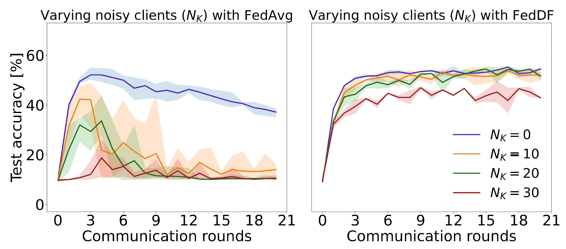
In order to simulate the fact that certain user devices may be untrustworthy, the notion of noisy clients was explored. For a noisy client, all labels in the training data were replaced with randomly chosen categories, effectively removing any valuable information. Subsequently, the performance was evaluated based on the number of noisy clients N K K , emulating the presence of malfunctioning or even hostile clients.
Suppose L N represents the set of noisy clients, where | L N | = N K , and D N denotes the training data for a noisy client. The process of converting the training data to noisy data can be expressed as below:
D N = ( x i , y i ) | ( x i , y i ) D , y i Uniform ( 1 , , l ) ,
where x i is the feature vector, y i is the original label, and y i is the substituted random label.

3.11. Evaluation Methodology

For the purpose of assessment, a series of experiments were conducted utilizing the FedAvg algorithm in order to investigate the influence of four key variables: the number of clients sampled (S), class balance ( α ), the number of local epochs (E), and the presence of noisy clients ( N K ). Furthermore, the FedDF algorithm was also employed for experiments concerning class balance and noisy clients.
Repetitions of experiments focusing on local epochs were executed on a physically federated network of Raspberry Pi devices, connected to the internet through both Ethernet and Wi-Fi. The choice of this specific parameter was made due to its influence on the runtime of each communication round, while the behaviors observed for other tested parameters remained largely consistent, regardless of whether the number of communication rounds or wall time was used as the x-axis. Apart from the particular parameter being varied in each experiment, all other experiments adhered to the baseline outlined in Table 2. The selection of these parameters was informed by existing research, particularly the works of [4,5], as well as some initial exploratory experimentation.

4. Analysis of Experimental Results

4.1. Previous Outcomes

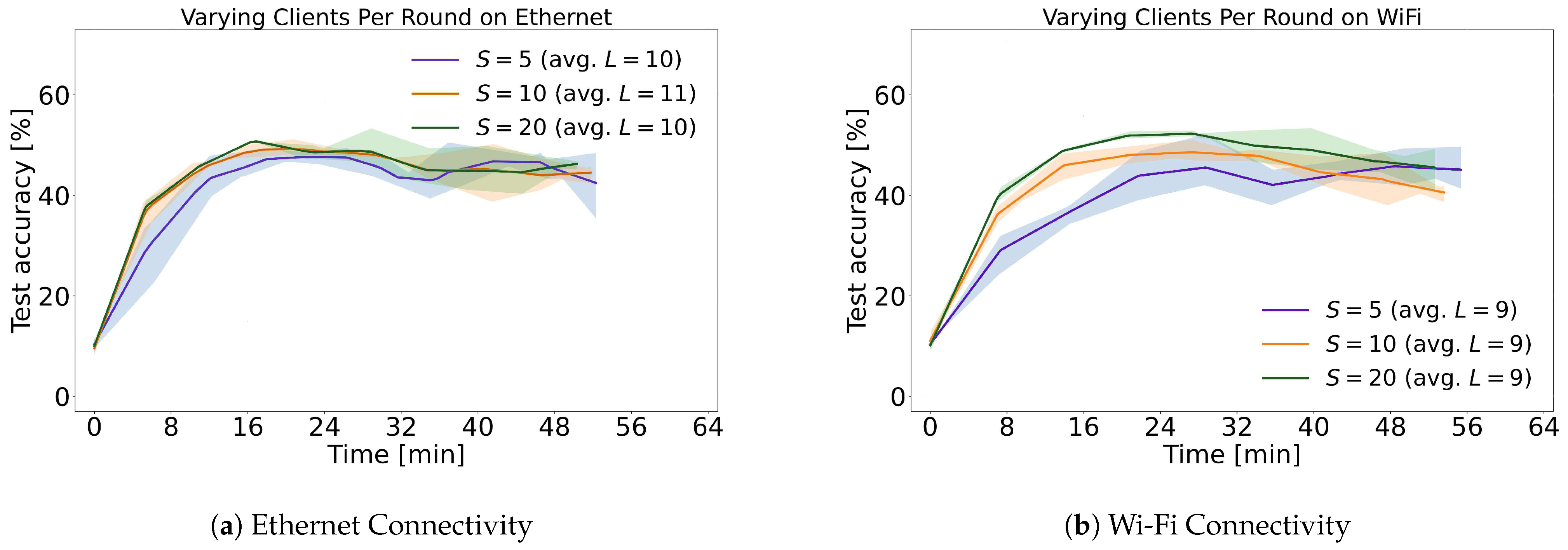
Figure 4 displays the experiments conducted using the Raspberry Pi system, which aimed to investigate the performance of federated learning algorithms in a real-world context. It is crucial to acknowledge that these tests were time-limited, which led to the execution of various communication cycles. The lines in the figure represent the average accuracy of three repetitions, while the shaded areas demonstrate the best and worst repetitions at any given point in time. Furthermore, the legend indicates the number of rounds (L) completed by each experiment before the 50 min timeout. Figure 5 exhibits the variations in clients per round over Ethernet and Wi-Fi connections.
The experimental setup aimed to provide insights into the impact of different communication methods on the performance of federated learning algorithms. This was carried out by examining the convergence behavior of models under varying network conditions, such as Ethernet and Wi-Fi connections, and different numbers of local epochs (E) and clients (S) per round.
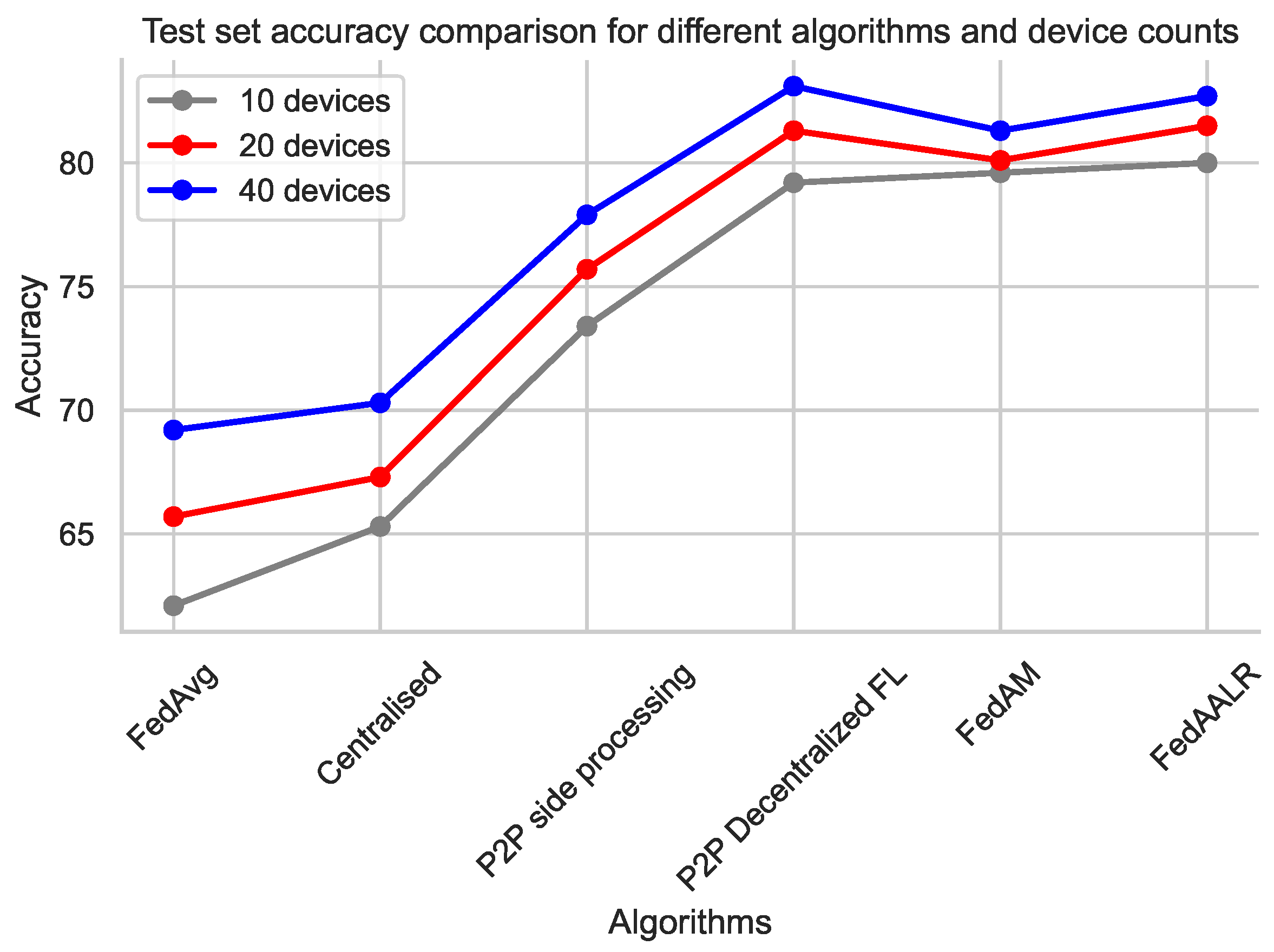
The results indicate that it is possible to achieve model convergence even when data are dispersed across multiple devices. This conclusion is supported by the observation that continuing the E = 1 training resulted in 65.3% centralized learning accuracy; the peer-to-peer side-processing method attained 73.4% and the peer-to-peer decentralized federated learning reached 79.2% accuracy, as outlined in Table 3.
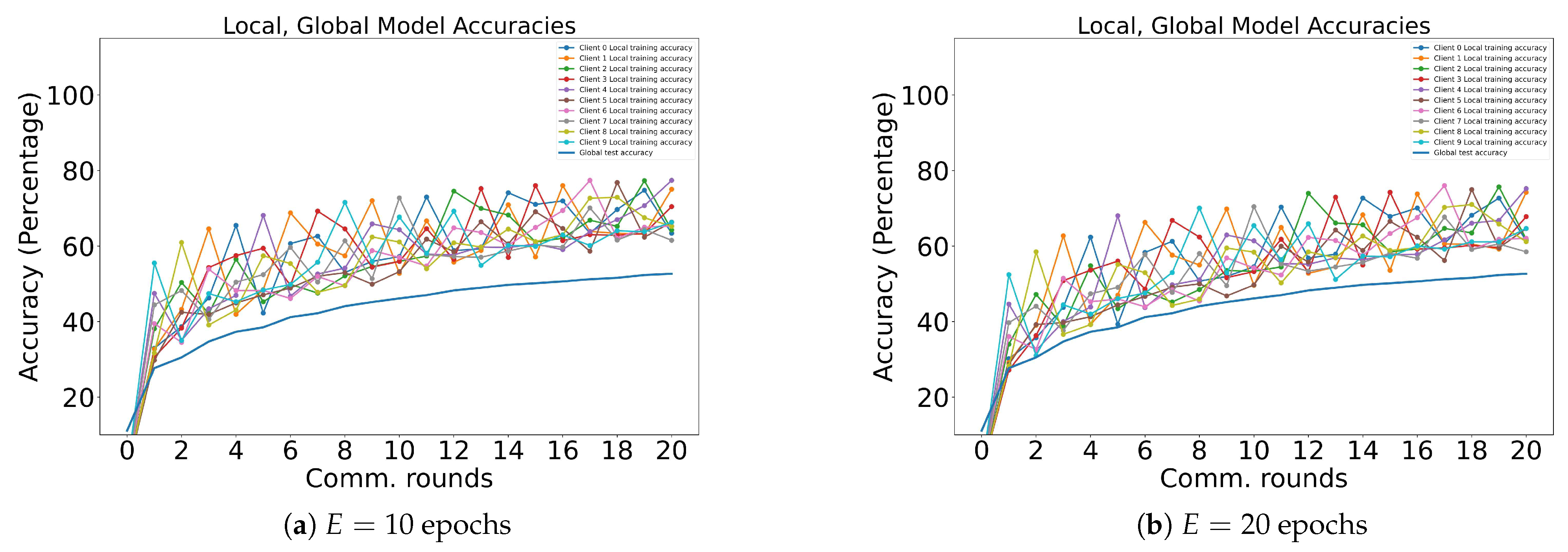
As illustrated in Figure 4, most accuracy curves tend to decline during the majority of the training phase. This effect becomes progressively more pronounced as the number of local epochs increases. This undesirable behavior can be attributed to overfitting. To validate this assertion, test performances during local epochs are presented in Figure 6b. During these epochs, the training accuracy of each client experiences a significant increase, while the overall training accuracy dramatically decreases. A direct countermeasure is to perform a systematic hyperparameter search, evaluating the efficacy of advanced regularization methods. A more comprehensive approach involves implementing local early stopping. However, devising such a rule is non-trivial, as there are cases where the global average model improves even when all local models overfit. This phenomenon is observed in early communication rounds and during the less biased learning for E = 10 , as displayed in Figure 6a.
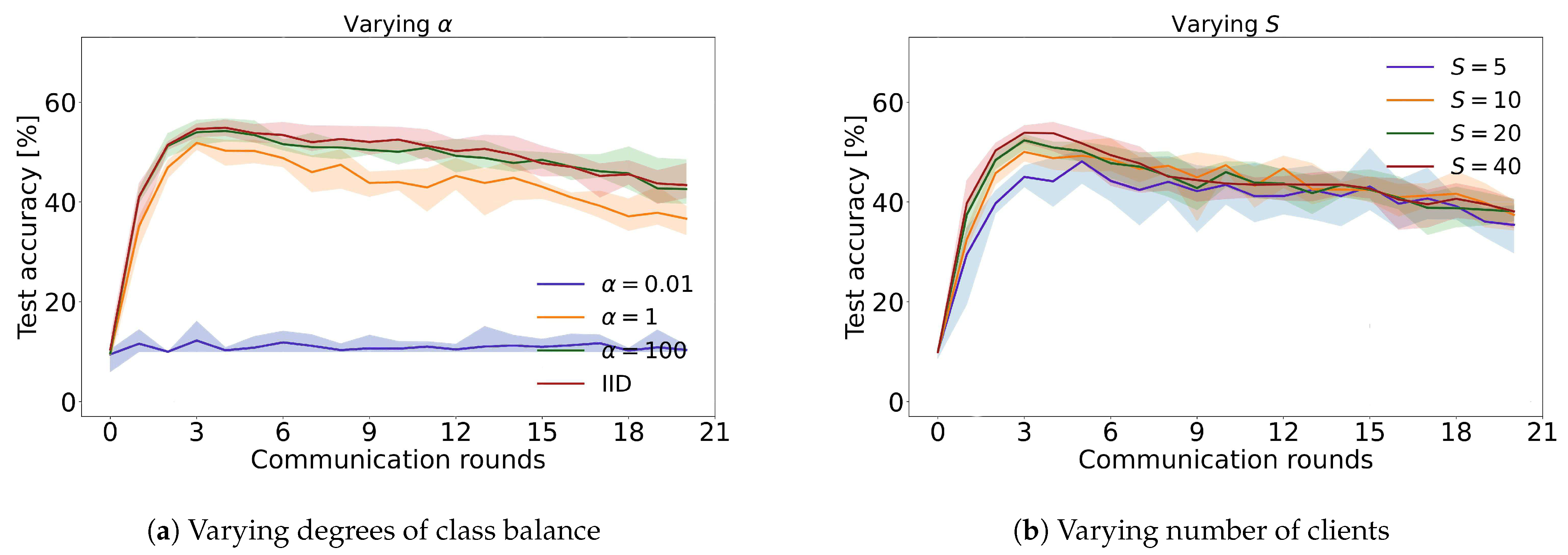
The experiments also aimed to explore the impact of various factors on federated learning performance, such as class balance (Figure 7a), the presence of noisy clients (Figure 8), as well as the number of clients sampled per round (Figure 7b). These analyses provide valuable insights into the challenges and potential solutions associated with implementing federated learning algorithms in real-world settings, where data may be imbalanced, noisy, or distributed across heterogeneous devices.
To summarize, the experimental results presented in this section offer valuable insights into the behavior of federated learning algorithms under different network conditions and configurations. These findings can help researchers and practitioners better understand the challenges associated with deploying federated learning algorithms in real-world settings and inform the development of more robust and efficient solutions to address these challenges.

4.2. Current Results

From Table 3, we can observe that both FedAM and FedAALR algorithms outperform FedAvg in terms of final accuracy and steps before convergence. In our experiment, we put into action the FedAvg algorithm, which employed a set value of E = 1 in addition to other standard parameters. In parallel, we also used a centralized learning algorithm. This method ensured complete training for each epoch while keeping in line with the optimization approach employed by federated learning (FL). The improvements were more significant when the number of devices increased. As we can observe, the P2P techniques have higher accuracy than the traditional methods; however, they require 200 communication rounds to reach that number, while FedAM and FedAALR require fewer. Note, also, that there are communication costs. P2P methods may require more communication between devices than FedAM or FedAALR, which can be a significant drawback in real-world settings, especially when network bandwidth is limited. Convergence speed is crucial too. While P2P side processing and P2P decentralized FL might achieve satisfactory accuracy, it’s not clear how quickly it converges compared to FedAM and FedAALR. The convergence rate, as determined by the number of communication rounds needed, is a crucial factor in evaluating the efficiency of federated learning algorithms. Additionally, scalability is a significant consideration, especially as the number of devices participating in the federated learning process increases, as it directly impacts the communication overhead in a peer-to-peer federated learning (P2PFL) setting. As the number of devices increases, the communication overhead for P2PFL may become prohibitive, while FedAM and FedAALR might scale better with more devices due to their centralized aggregation approach. In Figure 9, the results for the accuracy comparison across all methods are presented for 10, 20, and 40 Raspberry Pi devices.
As we can observe, the higher accuracy occurred on the P2P decentralized method, reaching 82% when it was deployed on 40 devices. The lower accuracy appeared on the FedAvg algorithm, 62% with 10 devices, while it increased to 69% with 40 devices. Satisfactory accuracy appeared on the newly introduced methods FedAM and FedAALR with 81.3% and 82.7% accuracy, respectively, when deployed over 40 devices. Note that this accuracy is reached with fewer communication rounds compared to the other methods.

5. Parameter Optimization in Federated Learning

5.1. Federated Averaging with Momentum

The Federated Averaging with Momentum (FedAM) algorithm presents opportunities for further performance improvement through parameter optimization. To identify optimal values for the input parameters, we analyzed the algorithm’s behavior with respect to its key parameters: the number of clients K, the number of selected clients per round S, the number of global rounds L, the number of local epochs E, the learning rate η , and the momentum coefficient β .
We started by investigating the learning rate η and momentum coefficient β . These parameters control the step size and the momentum term’s influence during the model update process. To find the optimal values, we could have used grid search, random search, or Bayesian optimization methods. For example, we could have set up a search space for η [ η min , η max ] and β [ β min , β max ] and used a chosen optimization method to find the optimal values that minimized the global objective function:
( η , β ) = arg min η , β F ( η , β ) ,
where F ( η , β ) is the global objective function, representing the global model’s performance on a validation dataset.
Next, we considered optimizing the number of clients K and the number of selected clients per round S. These parameters determine the trade-off between communication overhead and model convergence rate. Increasing S can accelerate convergence but may also increase communication costs. To optimize K and S, we defined a joint optimization problem with constraints on the communication overhead C:
( K , S ) = arg min K , S F ( K , S ) subject to C ( K , S ) C max ,
where C ( K , S ) is a function that measures the communication overhead and C max is the maximum allowable communication overhead.
The number of global rounds L and local epochs E affect the convergence speed and computation overhead. Increasing the number of local epochs E can reduce the communication rounds needed for convergence but may increase computation overhead. To optimize L and E, we defined a joint optimization problem with constraints on computation overhead T:
( L , E ) = arg min L , E F ( L , E ) subject to T ( L , E ) T max ,
where T ( L , E ) is a function that measures the computation overhead and T max is the maximum allowable computation overhead.
Finally, we combined all the optimization problems into a single multi-objective optimization problem, aiming to minimize the global objective function while satisfying the constraints on communication and computation overheads:
( η , β , K , S , L , E ) = arg min η , β , K , S , L , E F ( η , β , K , S , L , E ) subject to C ( K , S ) C max T ( L , E ) T max .

Incorporating Edge Caching and Bayesian Optimizations

To further improve the FedAM algorithm’s performance and efficiency, we incorporated edge caching techniques [53,54,55,56,57,58] and Bayesian optimization for hyperparameter tuning.
Edge Caching: To reduce communication overhead and latency, we utilized edge caching by caching model updates at the edge devices or edge servers. We introduced a caching factor α , where 0 α 1 , that represented the proportion of local updates to be cached at the edge device or edge server. The total communication overhead function C ( K , S ) was modified to account for the caching factor α :
C ( K , S , α ) = ( 1 α ) C ( K , S ) ,
We could then optimize the caching factor α by incorporating it into the optimization problem:
( K , S , α * ) = arg min K , S , α F ( K , S , α ) subject to C ( K , S , α ) C max ,
Bayesian Optimization: To efficiently search for the optimal hyperparameters, we employed Bayesian optimization, which modeled the objective function as a Gaussian process and used the acquisition function to guide the search. In this case, we defined the following optimization problem for hyperparameters:
( η , β , K , S , L , E , α * ) = arg min η , β , K , S , L , E , α F ( η , β , K , S , L , E , α ) subject to C ( K , S , α ) C max , T ( L , E ) T max
We iteratively updated the Gaussian process model and acquisition function, which balanced exploration and exploitation, to find the optimal hyperparameters.
In summary, this extended approach incorporates edge caching techniques to reduce communication overhead and latency, as well as Bayesian optimization for efficient hyperparameter tuning. These enhancements lead to improved performance, reduced communication costs, and accelerated convergence in federated learning settings.

5.2. Federated Averaging with Adaptive Learning Rates

In this section, we focus on parameter optimization in the context of the Federated Averaging with Adaptive Learning Rates (FedAALR) algorithm. By optimizing parameters, we achieve better model performance and faster convergence. We primarily rely on mathematical expressions to convey the ideas behind parameter optimization in this context.
The FedAALR algorithm involves several parameters, including the number of clients K, the fraction of clients S participating in each round, the number of global communication rounds L, the number of local epochs E, the initial learning rate η 0 , the cache decay rate γ , and the small constant for numerical stability ϵ . The optimal choice of these parameters depends on the specific problem, the network topology, and the characteristics of the clients’ datasets. The following discussion provides insights into optimizing these parameters:
  • Optimizing the initial learning rate η 0 : To optimize η 0 , we can minimize the validation loss L val ( η 0 ) with respect to η 0 . We can define a search space E = 0.1 ,   0.01 ,   0.001 ,   0.0001 and find the optimal learning rate as follows:
    η 0 * = arg min η 0 E L val ( η 0 ) ;
  • Optimizing the cache decay rate γ : To optimize γ , we can minimize the validation loss L val ( γ ) with respect to γ . We can define a search space G = 0.9 ,   0.99 ,   0.999 ,   0.9999 and find the optimal cache decay rate as follows:
    γ * = arg min γ G L val ( γ ) ;
  • Optimizing the number of clients K and fraction S : To optimize K and S, we can minimize the validation loss L val ( K , S ) with respect to K and S. We can define a search space K × S and find the optimal combination as follows:
    ( K , S ) = arg min ( K , S ) K × S L val ( K , S ) ;
  • Optimizing the number of global communication rounds L and local epochs E : To optimize L and E, we can minimize the validation loss L val ( L , E ) with respect to L and E. We can define a search space L × E and find the optimal combination as follows:
    ( L , E ) = arg min ( L , E ) L × E L val ( L , E ) .
These optimization equations serve as a guideline for selecting the optimal parameter values. However, depending on the specific problem and available computational resources, it may be necessary to employ additional heuristics, such as early stopping or Bayesian optimization, to improve the efficiency of the search process.

5.3. Incorporating Edge Caching and Bayesian Optimizations

Incorporating edge caching techniques into the FedAALR algorithm can help reduce communication costs and latency, making the algorithm more efficient. In this section, we discuss how edge caching can be integrated into the FedAALR algorithm and optimize the caching strategy:
  • Edge Caching: By caching intermediate model updates at the edge devices or edge servers, we can reduce the communication overhead between the clients and the central server. We introduce a caching factor α , where 0 α 1 , that represents the proportion of local updates to be cached at the edge device or edge server. We can modify the communication overhead function C ( K , S ) to account for the caching factor α :
    C ( K , S , α ) = ( 1 α ) C ( K , S ) .
    We can optimize the caching factor α by incorporating it into the optimization problem:
    ( K , S , α * ) = arg min K , S , α L val ( K , S , α ) subject to C ( K , S , α ) C max ;
  • Reducing Communication Costs: Communication costs can be reduced by adjusting the parameters of the FedAALR algorithm. For example, increasing the number of local epochs E can reduce the number of required communication rounds, thereby reducing communication costs. Additionally, adjusting the fraction of clients S participating in each round can also influence communication costs. To optimize the trade-off between communication costs and convergence speed, we can consider a joint optimization problem:
    ( E , S ) = arg min E , S L val ( E , S ) subject to C ( K , S , α ) C max ;
  • Other Optimizations: Apart from edge caching and communication cost reduction, other optimization techniques can be applied to the FedAALR algorithm. For instance, using adaptive communication strategies, where the frequency of communication between clients and the central server is adjusted based on the convergence rate, can help improve efficiency. Additionally, employing techniques such as gradient sparsification or quantization can further reduce communication overhead.
In summary, incorporating edge caching and optimizing communication costs can lead to significant improvements in the FedAALR algorithm’s efficiency and performance. Other optimization techniques, such as adaptive communication strategies and gradient compression, can also be considered to further enhance the algorithm’s effectiveness in federated learning scenarios.

6. In-Depth Analysis and Explanation

The comprehensive investigation into early learning on Raspberry Pi devices, which exhibit a reduced propensity for overfitting, implies that a smaller count of local epochs is not always beneficial. When constrained by training duration, for example, 5 to 15 min for Ethernet and 5 to 40 min for Wi-Fi, the ideal quantity of local epochs might grow. This phenomenon can be attributed to the increased number of local epochs contributing to a more significant amount of time spent on training and less time for communication, particularly evident on slower Wi-Fi connections. As a result, there is a tradeoff, where the value of E should not be excessively high, promoting overfitting, nor too low, hindering the speed of training data processing. When deciding on this value, professionals must take into account available training time and system communication latencies.
For a fixed number of rounds, without considering computational and communication impacts, E = 10 seems to strike the perfect equilibrium between underfitting and overfitting. With somewhat unbalanced datasets and α = 1 , FedAvg demonstrates consistent performance, independent of whether half or all clients are sampled. An overall accuracy of 62% was attained with a mere five clients per round, highlighting the reliability of model averaging. The difference is most apparent in the initial rounds, where smaller values of S result in slower convergence, as illustrated in Figure 7b. The lines depict the average performance of five repetitions, and the colored areas represent the least and most efficient repetitions for each run. Furthermore, Figure 7a showcases the different alphas.
Assessing class balancing results reveals that lowering α to 0.01 destabilizes the system, while training on α = 100 or iid improves learning. FedDF experiments with the same hyperparameters display superior performance. We hypothesize that distillation bypasses the adverse effects of overfitted local models by combining models without averaging across significant, bias-inducing factors. Figure 10 shows that FedDF prevents long-term performance decline. Empirical prediction probability distributions might offer a more accurate representation of acquired knowledge than model weights.
FedDF’s enhanced resilience is further evidenced in noise experiments, where 10 out of 40 data partitions being noisy substantially impairs FedAvg’s performance. In contrast, FedDF performs reasonably well even with 30 out of 40 noisy partitions. Averaging probabilities instead of model weights appears to mitigate the negative consequences of merging models with heterogeneous parameter values.
The latest outcomes in Table 3 include the performance of new techniques and the extension to 40 Raspberry Pi devices. The P2P Decentralized FL, FedAM, and FedAALR methods consistently surpass FedAvg and centralized learning across various device counts, suggesting that these strategies are more adept at addressing federated learning challenges. The P2P Decentralized FL method, in particular, demonstrates substantial improvements in accuracy, achieving 83.1% with 40 devices. These results underscore the potential of the P2P approach and other novel methods for enhancing federated learning performance, particularly when scaling up to larger numbers of devices.

7. Conclusions and Future Directions

This article delved into the possibilities of edge intelligence and distributed federated learning in Internet of Things (IoT) applications, elucidating the intricacies of the FedAvg and FedDF algorithms. We emphasized the viability of privacy-preserving learning on actual devices, taking into account communication efficiency and robustness against data imbalance in algorithmic selections. Moreover, we proposed two algorithms that transform the federated learning scenario into a peer-to-peer framework and presented two supplementary methods, FedAM and FedAALR, which exhibited promising performance enhancements.
Our experimental findings revealed that employing the straightforward yet potent FedAvg algorithm with an increased number of local training iterations on devices leads to pronounced overfitting, while fewer epochs incur elevated communication costs. Conversely, FedDF, a distillation aggregation approach, mitigates overfitting and augments tolerance to diverse data distributions, albeit at the expense of extra central server processing. We also introduced a client-balancing Dirichlet sampling strategy that guarantees equal sampling of each device, promoting fairness among all participating devices and precluding oversampled labels from skewing the overall dataset.
The two supplementary techniques introduced in this study, FedAM and FedAALR, demonstrated the potential for boosting federated learning performance on edge devices within IoT applications. Future research could entail assessing the suitability of FedAM and FedAALR for various learning tasks, fine-tuning their underlying algorithms, and pinpointing potential synergies with other federated learning methodologies.
As edge intelligence and distributed federated learning gain traction in IoT applications, a myriad of exciting research directions can be explored. These encompass examining numerous realistic learning tasks, such as high-performance computer vision models, and federating devices with more processing power than Raspberry Pi devices, such as smartphones. Another aspect worth investigating is managing datasets with erroneous or missing values, a prevalent issue in IoT settings.
Efficient sampling schemes, as suggested in [59,60,61,62], could further enhance the client-balancing method, although additional research is required. Lastly, the peer-to-peer scenarios presented for side processing and P2P–FL, in conjunction with [63], merit further scrutiny for potential optimization fine-tuning. As federated learning progresses, these future research avenues will contribute to the development of more effective, scalable, and resilient algorithms for distributed learning on edge devices in IoT applications, ultimately bolstering edge intelligence capabilities in an extensive array of real-world situations.

Author Contributions

A.K., C.K., K.C.G., D.T., K.O. and S.S. conceived of the idea, designed and performed the experiments, analysed the results, drafted the initial manuscript and revised the final manuscript. All authors have read and agreed to the published version of the manuscript.

Funding

This research has been co-financed by the European Regional Development Fund of the European Union and Greek national funds through the Operational Program Competitiveness, Entrepreneurship and Innovation, under the call Special Actions in aquaticfarming- industrial materials- open innovation in culture (project title: “Virtual street museum. Innovative techniques, methods and tools for documentation, protection and promotion of cultural heritage”: T6γBΠ-00534).

Data Availability Statement

The data presented in this study are available on request from the corresponding author.

Conflicts of Interest

The authors declare no conflict of interest.

Appendix A

Appendix A.1. Basic Notations and Symbols

The notations and symbols used in this work are summarized in Table A1.
Table A1. Basic Notations and Symbols.
SymbolDescription
KNumber of clients in the federated learning system
n k Size of the unique portion of the larger training dataset held by the k-th client
M G Global model hosted on the central server
LNumber of communication rounds
SNumber of clients selected for each communication round
ENumber of local epochs of learning performed by clients
M k Local model of the k-th client
fImplicit objective function
w Model weights
Loss function
M G ( l + 1 ) Updated global model after the l-th communication round
M k i ( l ) Updated local model of the i-th client after the l-th communication round
α Parameter vector for the Dirichlet distribution
π Probability distribution across labels
π i Label distribution for the i-th client
CNumber of clients (in the context of the Dirichlet sampling algorithm)
P Matrix representing the label distributions for all clients
S j Sum of the elements of the j-th column of matrix P
uMeasure to assess the closeness of P to the goal of equal column sums
λ Optional scaling factor for the measure u

Appendix A.2. Hardware Setup

The engineering part of this work is presented in Figure A1.
Figure A1. Hardware Setup Illustration.
Information 14 00414 g0a1

References

  1. Kairouz, P.; McMahan, H.B.; Avent, B.; Bellet, A.; Bennis, M.; Bhagoji, A.N.; Bonawitz, K.; Charles, Z.; Cormode, G.; Cummings, R.; et al. Advances and open problems in federated learning. Found. Trends Mach. Learn. 2021, 14, 1–210. [Google Scholar] [CrossRef]
  2. Blanco-Justicia, A.; Domingo-Ferrer, J.; Martínez, S.; Sánchez, D.; Flanagan, A.; Tan, K.E. Achieving security and privacy in federated learning systems: Survey, research challenges and future directions. Eng. Appl. Artif. Intell. 2021, 106, 104468. [Google Scholar] [CrossRef]
  3. Yang, Q.; Liu, Y.; Chen, T.; Tong, Y. Federated machine learning: Concept and applications. ACM Trans. Intell. Syst. Technol. (TIST) 2019, 10, 1–19. [Google Scholar] [CrossRef]
  4. McMahan, B.; Moore, E.; Ramage, D.; Hampson, S.; y Arcas, B.A. Communication-efficient learning of deep networks from decentralized data. In Proceedings of the Artificial Intelligence and Statistics (PMLR 2017), Sydney, NSW, Australia, 6–11 August 2017; pp. 1273–1282. [Google Scholar]
  5. Lin, T.; Kong, L.; Stich, S.U.; Jaggi, M. Ensemble distillation for robust model fusion in federated learning. Adv. Neural Inf. Process. Syst. 2020, 33, 2351–2363. [Google Scholar]
  6. Zhang, T.; Gao, L.; He, C.; Zhang, M.; Krishnamachari, B.; Avestimehr, A.S. Federated learning for the internet of things: Applications, challenges, and opportunities. IEEE Internet Things Mag. 2022, 5, 24–29. [Google Scholar] [CrossRef]
  7. Shaheen, M.; Farooq, M.S.; Umer, T.; Kim, B.S. Applications of federated learning; Taxonomy, challenges, and research trends. Electronics 2022, 11, 670. [Google Scholar] [CrossRef]
  8. Rodríguez-Barroso, N.; Jiménez-López, D.; Luzón, M.V.; Herrera, F.; Martínez-Cámara, E. Survey on federated learning threats: Concepts, taxonomy on attacks and defences, experimental study and challenges. Inf. Fusion 2023, 90, 148–173. [Google Scholar] [CrossRef]
  9. Rausch, T.; Dustdar, S. Edge intelligence: The convergence of humans, things, and ai. In Proceedings of the 2019 IEEE International Conference on Cloud Engineering (IC2E), Prague, Czech Republic, 24–27 June 2019; IEEE: Piscataway, NJ, USA, 2019; pp. 86–96. [Google Scholar]
  10. Wang, T.; Sun, B.; Wang, L.; Zheng, X.; Jia, W. EIDLS: An Edge-Intelligence-Based Distributed Learning System Over Internet of Things. IEEE Trans. Syst. Man Cybern. Syst. 2023, 1–13. [Google Scholar] [CrossRef]
  11. Britto Corthis, P.; Ramesh, G. A Journey of Artificial Intelligence and Its Evolution to Edge Intelligence. In Micro-Electronics and Telecommunication Engineering: Proceedings of 5th ICMETE 2021, Ghaziabad, India, 24–25 September 2022; Springer: Berlin/Heidelberg, Germany, 2022; pp. 817–826. [Google Scholar]
  12. Feng, H.; Mu, G.; Zhong, S.; Zhang, P.; Yuan, T. Benchmark analysis of yolo performance on edge intelligence devices. Cryptography 2022, 6, 16. [Google Scholar] [CrossRef]
  13. Wang, X.; Han, Y.; Leung, V.C.; Niyato, D.; Yan, X.; Chen, X. Edge AI: Convergence of Edge Computing and Artificial Intelligence; Springer: Berlin/Heidelberg, Germany, 2020. [Google Scholar]
  14. Liu, D.; Kong, H.; Luo, X.; Liu, W.; Subramaniam, R. Bringing AI to edge: From deep learning’s perspective. Neurocomputing 2022, 485, 297–320. [Google Scholar] [CrossRef]
  15. Du, Y.; Wang, Z.; Leung, V.C. Blockchain-enabled edge intelligence for IoT: Background, emerging trends and open issues. Future Internet 2021, 13, 48. [Google Scholar] [CrossRef]
  16. Molokomme, D.N.; Onumanyi, A.J.; Abu-Mahfouz, A.M. Edge intelligence in Smart Grids: A survey on architectures, offloading models, cyber security measures, and challenges. J. Sens. Actuator Netw. 2022, 11, 47. [Google Scholar] [CrossRef]
  17. Liu, J.; Xiang, J.; Jin, Y.; Liu, R.; Yan, J.; Wang, L. Boost precision agriculture with unmanned aerial vehicle remote sensing and edge intelligence: A survey. Remote Sens. 2021, 13, 4387. [Google Scholar] [CrossRef]
  18. Schizas, N.; Karras, A.; Karras, C.; Sioutas, S. TinyML for Ultra-Low Power AI and Large Scale IoT Deployments: A Systematic Review. Future Internet 2022, 14, 363. [Google Scholar] [CrossRef]
  19. Mills, J.; Hu, J.; Min, G. Communication-efficient federated learning for wireless edge intelligence in IoT. IEEE Internet Things J. 2019, 7, 5986–5994. [Google Scholar] [CrossRef] [Green Version]
  20. Ye, Y.; Li, S.; Liu, F.; Tang, Y.; Hu, W. EdgeFed: Optimized federated learning based on edge computing. IEEE Access 2020, 8, 209191–209198. [Google Scholar] [CrossRef]
  21. Mwase, C.; Jin, Y.; Westerlund, T.; Tenhunen, H.; Zou, Z. Communication-efficient distributed AI strategies for the IoT edge. Future Gener. Comput. Syst. 2022, 131, 292–308. [Google Scholar] [CrossRef]
  22. Zhang, T.; Wang, S.; Li, G.; Liu, F.; Zhu, G.; Wang, R. Accelerating edge intelligence via integrated sensing and communication. In Proceedings of the ICC 2022-IEEE International Conference on Communications, Seoul, Republic of Korea, 16–20 May 2022; IEEE: Piscataway, NJ, USA, 2022; pp. 1586–1592. [Google Scholar]
  23. Tang, S.; Chen, L.; He, K.; Xia, J.; Fan, L.; Nallanathan, A. Computational intelligence and deep learning for next-generation edge-enabled industrial IoT. IEEE Trans. Netw. Sci. Eng. 2022. [Google Scholar] [CrossRef]
  24. Shan, N.; Cui, X.; Gao, Z. “DRL+ FL”: An intelligent resource allocation model based on deep reinforcement learning for Mobile Edge Computing. Comput. Commun. 2020, 160, 14–24. [Google Scholar] [CrossRef]
  25. Abreha, H.G.; Hayajneh, M.; Serhani, M.A. Federated learning in edge computing: A systematic survey. Sensors 2022, 22, 450. [Google Scholar] [CrossRef] [PubMed]
  26. Dean, J.; Corrado, G.; Monga, R.; Chen, K.; Devin, M.; Mao, M.; Ranzato, M.; Senior, A.; Tucker, P.; Yang, K.; et al. Large scale distributed deep networks. Adv. Neural Inf. Process. Syst. 2012, 25, 1223–1231. [Google Scholar]
  27. McMahan, H.B.; Ramage, D.; Talwar, K.; Zhang, L. Learning differentially private recurrent language models. arXiv 2017, arXiv:1710.06963. [Google Scholar]
  28. Bonawitz, K.; Ivanov, V.; Kreuter, B.; Marcedone, A.; McMahan, H.B.; Patel, S.; Ramage, D.; Segal, A.; Seth, K. Practical secure aggregation for privacy-preserving machine learning. In Proceedings of the 2017 ACM SIGSAC Conference on Computer and Communications Security, Dallas, TX, USA, 30 October–3 November 2017; pp. 1175–1191. [Google Scholar]
  29. Karras, A.; Karras, C.; Giotopoulos, K.C.; Tsolis, D.; Oikonomou, K.; Sioutas, S. Peer to Peer Federated Learning: Towards Decentralized Machine Learning on Edge Devices. In Proceedings of the 2022 7th South-East Europe Design Automation, Computer Engineering, Computer Networks and Social Media Conference (SEEDA-CECNSM), Ioannina, Greece, 23–25 September 2022; pp. 1–9. [Google Scholar] [CrossRef]
  30. Wang, X.; Chen, W.; Xia, J.; Wen, Z.; Zhu, R.; Schreck, T. HetVis: A Visual Analysis Approach for Identifying Data Heterogeneity in Horizontal Federated Learning. IEEE Trans. Vis. Comput. Graph. 2023, 29, 310–319. [Google Scholar] [CrossRef] [PubMed]
  31. Wang, J.; Zhang, L.; Li, A.; You, X.; Cheng, H. Efficient Participant Contribution Evaluation for Horizontal and Vertical Federated Learning. In Proceedings of the 2022 IEEE 38th International Conference on Data Engineering (ICDE), Kuala Lumpur, Malaysia, 9–12 May 2022; IEEE: Piscataway, NJ, USA, 2022; pp. 911–923. [Google Scholar]
  32. Zhang, X.; Mavromatics, A.; Vafeas, A.; Nejabati, R.; Simeonidou, D. Federated Feature Selection for Horizontal Federated Learning in IoT Networks. IEEE Internet Things J. 2023, 10, 10095–10112. [Google Scholar] [CrossRef]
  33. Aono, Y.; Hayashi, T.; Wang, L.; Moriai, S. Privacy-preserving deep learning via additively homomorphic encryption. IEEE Trans. Inf. Forensics Secur. 2017, 13, 1333–1345. [Google Scholar]
  34. Chen, Y.R.; Rezapour, A.; Tzeng, W.G. Privacy-preserving ridge regression on distributed data. Inf. Sci. 2018, 451, 34–49. [Google Scholar] [CrossRef]
  35. Kim, H.; Park, J.; Bennis, M.; Kim, S.L. On-device federated learning via blockchain and its latency analysis. arXiv 2018, arXiv:1808.03949. [Google Scholar]
  36. Islam, A.; Al Amin, A.; Shin, S.Y. FBI: A Federated Learning-Based Blockchain-Embedded Data Accumulation Scheme Using Drones for Internet of Things. IEEE Wirel. Commun. Lett. 2022, 11, 972–976. [Google Scholar] [CrossRef]
  37. Smith, V.; Chiang, C.K.; Sanjabi, M.; Talwalkar, A.S. Federated multi-task learning. Adv. Neural Inf. Process. Syst. 2017, 30, 4424–4434. [Google Scholar]
  38. Du, W.; Han, Y.S.; Chen, S. Privacy-preserving multivariate statistical analysis: Linear regression and classification. In Proceedings of the 2004 SIAM International Conference on Data Mining, Lake Buena Vista, FL, USA, 22–24 April 2004; pp. 222–233. [Google Scholar]
  39. Du, W.; Atallah, M.J. Privacy-preserving cooperative statistical analysis. In Proceedings of the Seventeenth Annual Computer Security Applications Conference, New Orleans, LA, USA, 10–14 December 2001; IEEE: Piscataway, NJ, USA, 2001; pp. 102–110. [Google Scholar]
  40. Wan, L.; Ng, W.K.; Han, S.; Lee, V.C. Privacy-preservation for gradient descent methods. In Proceedings of the 13th ACM SIGKDD International Conference on Knowledge Discovery and Data Mining, San Jose, CA, USA, 12–15 August 2007; pp. 775–783. [Google Scholar]
  41. Karr, A.F.; Lin, X.; Sanil, A.P.; Reiter, J.P. Privacy-preserving analysis of vertically partitioned data using secure matrix products. J. Off. Stat. 2009, 25, 125. [Google Scholar]
  42. Vaidya, J.; Clifton, C. Privacy preserving association rule mining in vertically partitioned data. In Proceedings of the Eighth ACM SIGKDD International Conference on Knowledge Discovery and Data Mining, Edmonton, AB, Canada, 23–26 July 2002; pp. 639–644. [Google Scholar]
  43. Cheng, K.; Fan, T.; Jin, Y.; Liu, Y.; Chen, T.; Papadopoulos, D.; Yang, Q. Secureboost: A lossless federated learning framework. IEEE Intell. Syst. 2021, 36, 87–98. [Google Scholar] [CrossRef]
  44. Hardy, S.; Henecka, W.; Ivey-Law, H.; Nock, R.; Patrini, G.; Smith, G.; Thorne, B. Private federated learning on vertically partitioned data via entity resolution and additively homomorphic encryption. arXiv 2017, arXiv:1711.10677. [Google Scholar]
  45. Schoenmakers, B.; Tuyls, P. Efficient binary conversion for Paillier encrypted values. In Advances in Cryptology-EUROCRYPT 2006: Proceedings of the 24th Annual International Conference on the Theory and Applications of Cryptographic Techniques, St. Petersburg, Russia, 28 May–1 June 2006; Springer: Berlin/Heidelberg, Germany, 2006; pp. 522–537. [Google Scholar]
  46. Xu, D.; Li, T.; Li, Y.; Su, X.; Tarkoma, S.; Jiang, T.; Crowcroft, J.; Hui, P. Edge Intelligence: Empowering Intelligence to the Edge of Network. Proc. IEEE 2021, 109, 1778–1837. [Google Scholar] [CrossRef]
  47. Liu, T.; Di, B.; Song, L. Privacy-Preserving Federated Edge Learning: Modeling and Optimization. IEEE Commun. Lett. 2022, 26, 1489–1493. [Google Scholar] [CrossRef]
  48. Mora, A.; Fantini, D.; Bellavista, P. Federated Learning Algorithms with Heterogeneous Data Distributions: An Empirical Evaluation. In Proceedings of the 2022 IEEE/ACM 7th Symposium on Edge Computing (SEC), Seattle, WA, USA, 5–8 December 2022; IEEE: Piscataway, NJ, USA, 2022; pp. 336–341. [Google Scholar]
  49. Jin, C.; Chen, X.; Gu, Y.; Li, Q. FedDyn: A dynamic and efficient federated distillation approach on Recommender System. In Proceedings of the 2022 IEEE 28th International Conference on Parallel and Distributed Systems (ICPADS), Nanjing, China, 10–12 January 2023; IEEE: Piscataway, NJ, USA, 2023; pp. 786–793. [Google Scholar]
  50. Cui, J.; Wu, Q.; Zhou, Z.; Chen, X. FedBranch: Heterogeneous Federated Learning via Multi-Branch Neural Network. In Proceedings of the 2022 IEEE/CIC International Conference on Communications in China (ICCC), Sanshui, Foshan, China, 11–13 August 2022; IEEE: Piscataway, NJ, USA, 2022; pp. 1101–1106. [Google Scholar]
  51. Li, N.; Wang, N.; Ou, W.; Han, W. FedTD: Efficiently Share Telemedicine Data with Federated Distillation Learning. In International Conference on Machine Learning for Cyber Security; Springer: Berlin/Heidelberg, Germany, 2023; pp. 501–515. [Google Scholar]
  52. Yang, Y.; Yang, R.; Peng, H.; Li, Y.; Li, T.; Liao, Y.; Zhou, P. FedACK: Federated Adversarial Contrastive Knowledge Distillation for Cross-Lingual and Cross-Model Social Bot Detection. arXiv 2023, arXiv:2303.07113. [Google Scholar]
  53. Musa, S.S.; Zennaro, M.; Libsie, M.; Pietrosemoli, E. Mobility-aware proactive edge caching optimization scheme in information-centric iov networks. Sensors 2022, 22, 1387. [Google Scholar] [CrossRef]
  54. Li, C.; Qianqian, C.; Luo, Y. Low-latency edge cooperation caching based on base station cooperation in SDN based MEC. Expert Syst. Appl. 2022, 191, 116252. [Google Scholar] [CrossRef]
  55. Qian, L.; Qu, Z.; Cai, M.; Ye, B.; Wang, X.; Wu, J.; Duan, W.; Zhao, M.; Lin, Q. FastCache: A write-optimized edge storage system via concurrent merging cache for IoT applications. J. Syst. Archit. 2022, 131, 102718. [Google Scholar] [CrossRef]
  56. Sharma, S.; Peddoju, S.K. IoT-Cache: Caching Transient Data at the IoT Edge. In Proceedings of the 2022 IEEE 47th Conference on Local Computer Networks (LCN), Edmonton, AB, Canada, 26–29 September 2022; IEEE: Piscataway, NJ, USA, 2022; pp. 307–310. [Google Scholar]
  57. Zhang, Z.; Wei, X.; Lung, C.H.; Zhao, Y. iCache: An Intelligent Caching Scheme for Dynamic Network Environments in ICN-based IoT Networks. IEEE Internet Things J. 2022, 10, 1787–1799. [Google Scholar] [CrossRef]
  58. Reiss-Mirzaei, M.; Ghobaei-Arani, M.; Esmaeili, L. A Review on the Edge Caching Mechanisms in the Mobile Edge Computing: A Social-aware Perspective. Internet Things 2023, 22, 100690. [Google Scholar] [CrossRef]
  59. Karras, C.; Karras, A.; Avlonitis, M.; Sioutas, S. An Overview of MCMC Methods: From Theory to Applications. In Artificial Intelligence Applications and Innovations, Proceedings of the AIAI 2022 IFIP WG 12.5 International Workshops: MHDW 2022, 5G-PINE 2022, AIBMG 2022, ML@ HC 2022, and AIBEI 2022, Hersonissos, Crete, Greece, 17–20 June 2022; Maglogiannis, I., Iliadis, L., Macintyre, J., Cortez, P., Eds.; Springer: Cham, Switzerland, 2022; pp. 319–332. [Google Scholar]
  60. Karras, C.; Karras, A.; Avlonitis, M.; Giannoukou, I.; Sioutas, S. Maximum Likelihood Estimators on MCMC Sampling Algorithms for Decision Making. In Artificial Intelligence Applications and Innovations, Proceedings of the AIAI 2022 IFIP WG 12.5 International Workshops: MHDW 2022, 5G-PINE 2022, AIBMG 2022, ML@ HC 2022, and AIBEI 2022, Hersonissos, Crete, Greece, 17–20 June 2022; Maglogiannis, I., Iliadis, L., Macintyre, J., Cortez, P., Eds.; Springer: Cham, Switzerland, 2022; pp. 345–356. [Google Scholar]
  61. Coullon, J.; South, L.; Nemeth, C. Efficient and generalizable tuning strategies for stochastic gradient MCMC. Stat. Comput. 2023, 33, 66. [Google Scholar] [CrossRef]
  62. Ding, S.; Li, C.; Xu, X.; Ding, L.; Zhang, J.; Guo, L.; Shi, T. A Sampling-Based Density Peaks Clustering Algorithm for Large-Scale Data. Pattern Recognit. 2023, 136, 109238. [Google Scholar] [CrossRef]
  63. Karras, A.; Karras, C.; Giotopoulos, K.C.; Giannoukou, I.; Tsolis, D.; Sioutas, S. Download Speed Optimization in P2P Networks Using Decision Making and Adaptive Learning. In Proceedings of the ICR’22 International Conference on Innovations in Computing Research, Athens, Greece, 29–31 August 2022; Daimi, K., Al Sadoon, A., Eds.; Springer International Publishing: Cham, Switezerland, 2022; pp. 225–238. [Google Scholar]
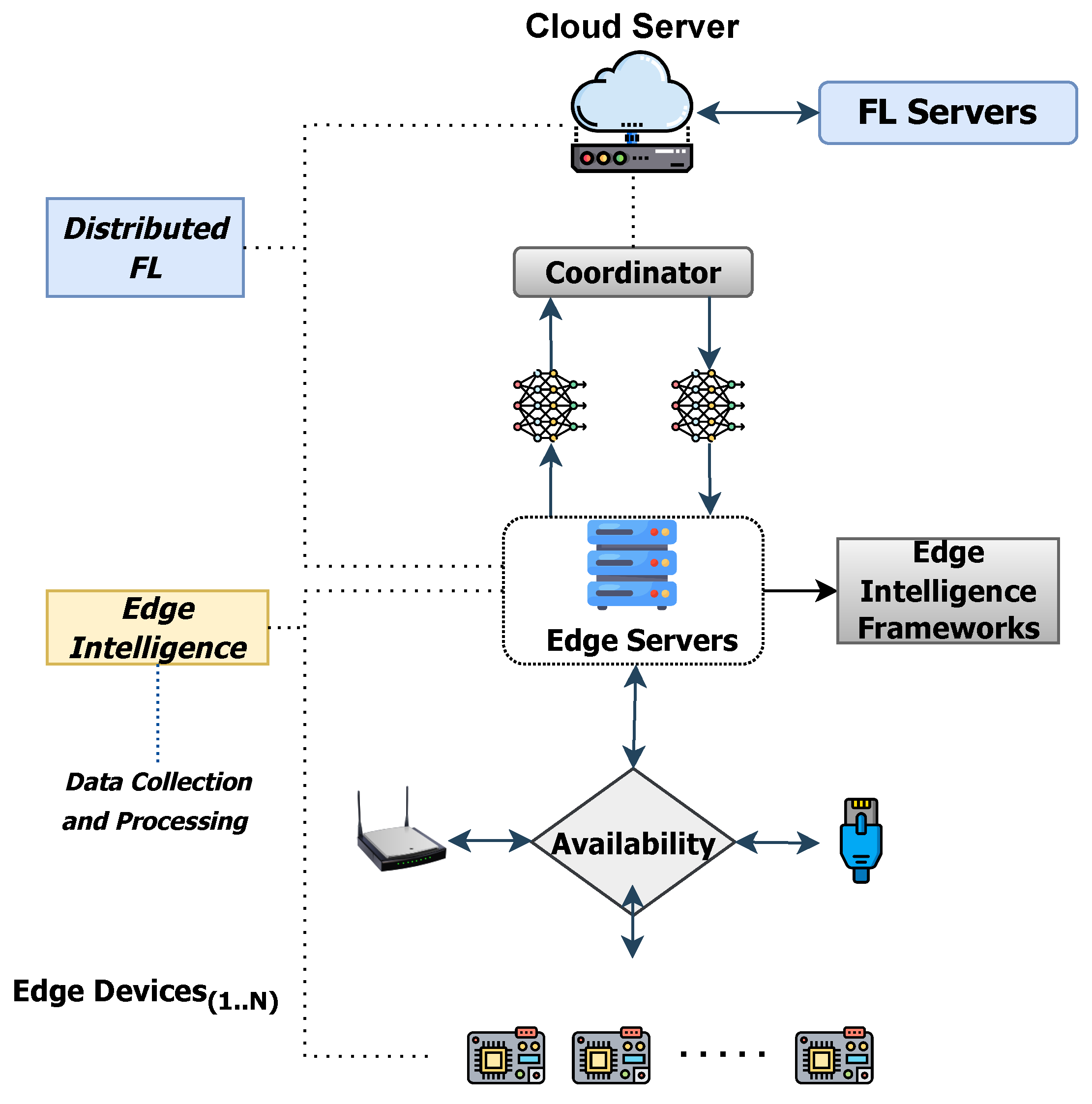
Figure 1. Architecture of Distributed Federated Learning with Edge Intelligence.
Information 14 00414 g001
Figure 2. Federated Learning Schema.
Information 14 00414 g002
Figure 3. The federated setup performing updates at communication round l, at which S 40 clients are sampled.
Information 14 00414 g003
Figure 4. Influence of varying local epochs (E) on the performance of the Raspberry Pi setup, comparing ethernet (left) and Wi-Fi (right) connectivity.
Information 14 00414 g004
Figure 5. Consequences of altering the number of participating clients (S) using the Raspberry Pi setup, contrasting Ethernet (left) and Wi-Fi (right) connections.
Information 14 00414 g005
Figure 6. Training progress captured by tracking accuracies for each client during each communication round, with faint lines signifying E = 10 local epochs (left) and E = 20 local epochs (right) completed by the selected clients.
Information 14 00414 g006
Figure 7. Evaluation of the global model’s performance on the test set across diverse communication rounds, considering varying degrees of class balance, denoted by α (left), and considering the impact of different numbers of clients sampled per round, denoted by S (right).
Information 14 00414 g007
Figure 8. Assessment of the global model’s performance on the test set throughout communication rounds, considering various levels of noisy clients ( N k ), comparing the outcomes of FedAvg (left) and FedDF (right) approaches.
Information 14 00414 g008
Figure 9. Test accuracy for all algorithms and devices.
Information 14 00414 g009
Figure 10. Comparison of FedAvg (left) and FedDF (right) under varying data imbalance: Test set performance over communication rounds.
Information 14 00414 g010
Table 1. Methods in Federated Learning: Advantages and Limitations.
MethodAdvantagesLimitations
Horizontal FLPrivacy preservation, accuracy enhancementInformation leak risk
Vertical FLFL performance improvement, privacy preservationNeeds novel solutions
Edge Intelligence with FLLow latency, bandwidth economy, privacy/securityExtensive research required
Table 2. Baseline parameters used for all experiments. Here, B denotes the training batch size.
KS α EL N K B η γ
4010–4012020016 5 · 10 4 0.995
Table 3. Algorithm execution persisted until a three-step stagnation in test set accuracy was observed.
AlgorithmStepsAccuracy (10 Devices)Accuracy (20 Devices)Accuracy (40 Devices)
FedAvg200 comm. rounds62.165.769.2
Centralized10 full epochs65.367.370.3
P2P side processing10 full epochs73.475.777.9
P2P Decentralized FL200 comm. rounds79.281.383.1
FedAM150 comm. rounds79.680.181.3
FedAALR130 comm. rounds80.081.582.7
Disclaimer/Publisher’s Note: The statements, opinions and data contained in all publications are solely those of the individual author(s) and contributor(s) and not of MDPI and/or the editor(s). MDPI and/or the editor(s) disclaim responsibility for any injury to people or property resulting from any ideas, methods, instructions or products referred to in the content.