Article

The Detection of COVID-19 in Chest X-rays Using Ensemble CNN Techniques

by
Domantas Kuzinkovas
and
Sandhya Clement
*
School of Biomedical Engineering, The University of Sydney, Sydney, NSW 2006, Australia
*
Author to whom correspondence should be addressed.
Information 2023, 14(7), 370; https://doi.org/10.3390/info14070370
Submission received: 22 May 2023 / Revised: 23 June 2023 / Accepted: 27 June 2023 / Published: 29 June 2023

Abstract

:
Advances in the field of image classification using convolutional neural networks (CNNs) have greatly improved the accuracy of medical image diagnosis by radiologists. Numerous research groups have applied CNN methods to diagnose respiratory illnesses from chest X-rays and have extended this work to prove the feasibility of rapidly diagnosing COVID-19 with high degrees of accuracy. One issue in previous research has been the use of datasets containing only a few hundred images of chest X-rays containing COVID-19, causing CNNs to overfit the image data. This leads to lower accuracy when the model attempts to classify new images, as would be clinically expected. In this work, we present a model trained on the COVID-QU-Ex dataset containing 33,920 chest X-ray images, with an equal share of COVID-19, Non-COVID pneumonia, and Normal images. The model is an ensemble of pre-trained CNNs (ResNet50, VGG19, and VGG16) and GLCM textural features. The model achieved a 98.34% binary classification accuracy (COVID-19/no COVID-19) on a test dataset of 6581 chest X-rays and 94.68% for distinguishing between COVID-19, Non-COVID pneumonia, and normal chest X-rays. The results also demonstrate that a higher 98.82% three-class test accuracy can be achieved using the model if the training dataset only contains a few thousand images. However, the generalizability of the model suffers due to the smaller dataset size. This study highlights the benefits of both ensemble CNN techniques and larger dataset sizes for medical image classification performance.

1. Introduction

Rapid diagnosis of COVID-19 in hospitals is vital for ensuring that patients with respiratory symptoms are triaged swiftly and receive the correct treatment. The state of the art for confirming a suspected COVID-19 case is using Reverse Transcriptase Polymerase Chain Reaction (RT-PCR). However, the process of obtaining PCR results is slow, and some studies have found it to be only sensitive to about 90.7% [1]. One alternative is to perform a chest X-ray, which takes 10 min or less, and then use a deep learning model to diagnose the patient, which takes milliseconds. Deep learning models are also typically more sensitive at detecting diseases from medical images than radiologists [2]. As this work will show, they can be more sensitive to detecting COVID-19 than a PCR.
Ever since the beginning of the COVID-19 pandemic, deep learning approaches for detecting coronavirus pneumonia in chest X-rays and its distinction from alternative pneumonia have become of great interest to the research community. Several groups have presented promising results using variations of convolutional neural network (CNN) based image recognition models [3,4,5,6,7,8,9,10].
Some models utilize only a single CNN for classification, such as in Wang et al. (2020), where a custom 89-layer CNN named COVID-Net was developed [3]. The group obtained a 93.3% accuracy for distinguishing between chest X-rays containing COVID-19 pneumonia, other pneumonia, or no condition. However, due to the novelty of the pandemic at the time, only 358 of the total 13,975 X-rays the group obtained were examples of a COVID-19 infection, making effective training of the model difficult due to the image class bias. Nevertheless, developing a custom CNN to perform medical image diagnoses is not exclusively required. Instead, a process known as transfer learning can be used, in which the feature extraction ability learned by a CNN trained on a different dataset can be transferred to assist in classifying images from a different application [4]. Zouch et al. (2022) employed a CNN transfer learning approach, comparing the performance of the ResNet50 and VGG19 CNNs pretrained on the ImageNet dataset [5]. VGG19 had superior performance between the two models, with a 99.35% binary classification accuracy (COVID-19/No COVID-19) compared to the 96.77% accuracy for ResNet50. However, due to the small and unbalanced dataset size of 112 COVID-19 and 747 Non-COVID-19 chest X-rays, overfitting of the dataset may have feasibly occurred. Despite this, the study conveys the effectiveness of transfer learning in a medical image classification application, proving that CNNs do not have to be built from scratch to obtain high classification accuracies.
CNNs do not have to be used for the classification step but can alternatively be utilized as feature extraction tools before passing these features to other types of classifiers [6,7,8,9,10]. Sethy et al. (2020) achieved a 4-class accuracy of 95.33% by combining ResNet50 with a Support Vector Machine (SVM) classifier [7]. Karim et al. (2022) combined the features extracted using AlexNet with several types of machine learning classifiers. They obtained a maximum three-class accuracy of 98.01% by transferring these features to a Naïve-Bayes classifier [9].
Models with more complex construction have been shown to achieve very high accuracies on medium-sized datasets. Notably, the methods of Mostafiz et al. (2022) included watershed segmentation, Gray Level Co-occurrence Matrix (GLCM)/Wavelet feature extraction, ResNet50 for feature extraction, feature selection using Maximum Relevance Minimum Redundancy (mRMR) and Recursive Feature Elimination (RFE), and a final Random Forest Classifier for classification [6]. Due to the high number of optimization steps, the accuracy obtained was 98.48% for a 4-class classification (COVID-19, Bacterial Pneumonia, Viral Pneumonia, and Normal). Their dataset was a combination of previous existing datasets, with 4809 chest X-rays, 790 of which contained COVID-19 infections.
Another example of this is in Toğaçar et al. (2020), where three CNNs were used to extract features from 5849 chest X-rays of positive and negative pneumonia cases [10]. An mRMR feature selection algorithm was used to determine the most important features. The group concluded that the best configuration involved selecting 100 features from each CNN before passing them to a Linear Discriminant Analysis (LDA) classifier. This configuration obtained a 99.41% binary classification accuracy. The benefit of such a system is that the classification outcome is a collaborative effort of several CNNs of different architectures, meaning that another CNN may account for features missed by one CNN.
The discussed literature provides great insight into the variety of viable models for classifying chest X-ray images. However, due to the novelty of COVID-19 at the time, the number of COVID-19 chest X-rays utilized by the studies did not exceed 3616 [9], and most only had below 1000. Many of these papers also present high (>98%) accuracies in the classification of chest X-rays. Great care must be taken when using smaller datasets to avoid the issue of overfitting. Dataset overfitting is the phenomenon whereby a classifier performs poorly on datasets that were not used to train it. It is often the result of not having enough training images to teach the classifier to extract generalized features from images of each class. Instead, it learns to extract features specific to the given dataset and performs worse when it cannot find these features in other datasets. This issue is far from trivial since clinical use of such a chest X-ray classification system requires that it be robust and accurate, no matter the X-ray image’s source or properties.
Many of the discussed studies did not explore the generalizability of their models on datasets external to their training datasets, preventing knowledge of their clinical effectiveness. In the present study, we train our model on a dataset containing almost 33,000 images in total, a third of which are COVID-19 infections, and we show that this has a marked improvement in generalizability performance compared to training on a smaller external dataset. We also expand on previous works by combining features from multiple CNNs with GLCM features. We also explore the relative benefits of RF, LDA, LR, and ANN classifiers to classify the combined features.

2. Materials and Methods

2.1. Datasets

The dataset used for training and evaluating the model was the COVID-QU-Ex dataset developed by researchers at Qatar University and the University of Dhaka [11,12,13] and obtained from various sources [14,15,16,17,18,19,20,21]. This dataset has 33,920 chest X-rays, of which 11,956 contain a COVID-19 infection, 11,263 contain bacterial or viral infections, and 10,701 are normal. This dataset was chosen for its large size and balanced nature, which help tackle overfitting and biased learning, respectively. Prior to using the dataset, it was cleaned by removing poor-quality X-rays. Some of the images in the COVID-QU-Ex dataset were cropped X-ray images with a black border, such that the actual X-ray formed a very small proportion of the 256 × 256 image frame. In others, the X-rays were of poor quality due to scatter, which clouded the lung regions with white pixels and decreased the overall contrast of the image. To eliminate these poorer-quality images, a program was run to remove images that contained either (1) more than 25% of pixel intensities less than 10 (near pure black) or (2) more than 15% of pixel values greater than 240 (near pure white). These values were chosen by examining histograms of visually deemed poor-quality images. This cleaning process lowered the number of images in the training set from 21,715 to 21,102, the validation set from 5417 to 5274, and the test set from 6788 to 6581. Examples of X-rays from each class can be found in Figure 1.
To explore the issue of overfitting in medical image literature, a smaller dataset of 4809 chest X-ray images was also obtained from Mostafiz et al. (2022) [6,22]. It contains 790 cases of COVID-19, 2519 cases of bacterial or viral pneumonia, and 1500 normal cases. It is actually composed of three datasets: COVID-19 images from Cohen et al. (2020) [23] and Dadario (2020) [24], and normal and pneumonia images from Kermany et al. (2018) [25]. A summary of the dataset statistics can be found in Table 1.

2.2. Model Overview

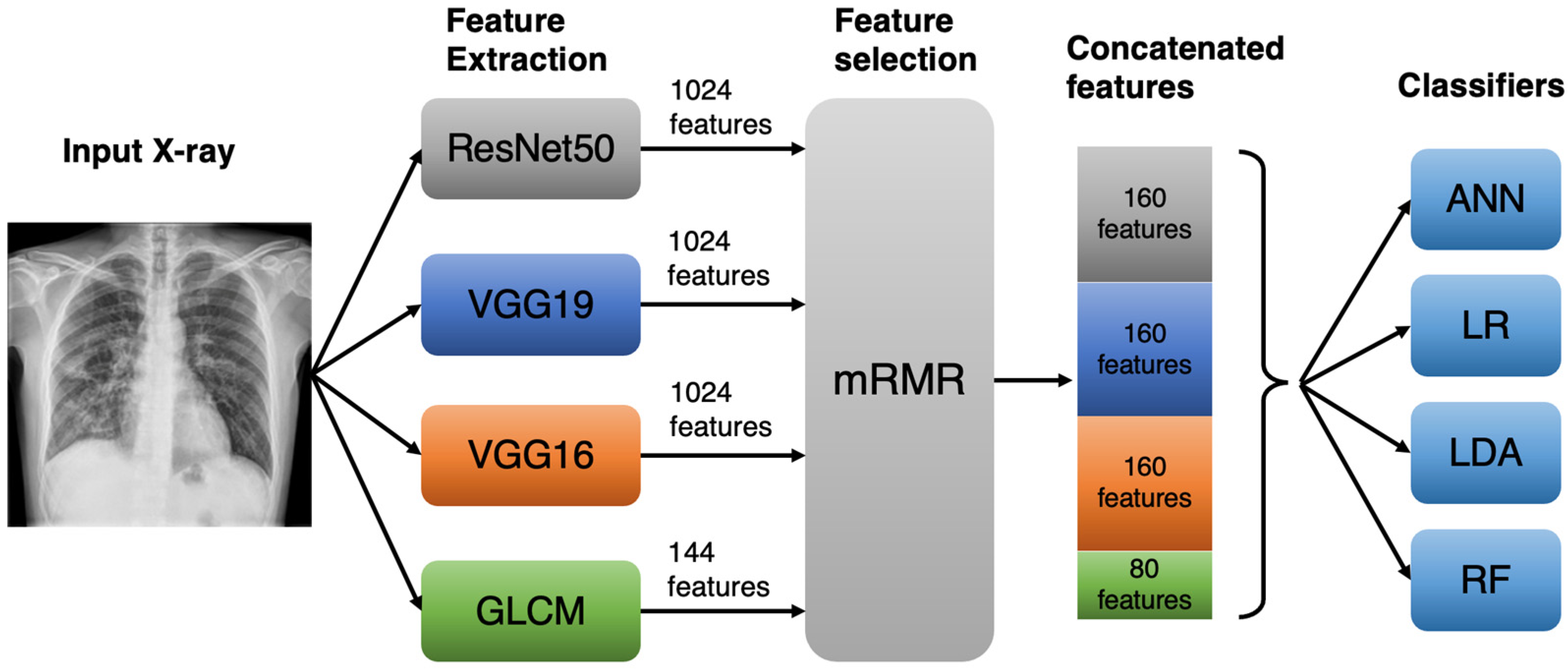
The model, illustrated in Figure 2, is a modification of the model used by Toğaçar et al. (2020) [10] and adapted for use in COVID-19 detection. It involves the combination of features extracted using several CNNs, in this case ResNet50, VGG19, and VGG16, and extracted GLCM features. The CNN features for one image consist of a vector of 1024 output values from the final Dense layer of each CNN, the layer immediately before the classification into the three image classes. The 80 GLCM features extracted from the Grey-Level Co-occurrence Matrix give details about textural features in the image, such as pixel contrast, energy, homogeneity, and correlation.
The 1024-value feature vectors from the CNNs are then shortened to vectors of only the 160 most important features for correctly classifying the chest X-ray. For GLCM features, 80 of 144 were selected. The selection criteria were determined by an mRMR (Minimum Redundancy Maximum Relevance) algorithm, available as a library in Python [26]. The purpose of performing this feature selection is to minimize computation time and prevent less irrelevant features from causing incorrect classifications.
Once the feature selection was performed, the 560 total features were concatenated. This vector was passed to one of the multiple traditional classifiers, including an Artificial Neural Network (ANN), Logistic Regression model (LR), Linear Discriminant Analysis (LDA), and Random Forest (RF) classifier, to fit the classification model. A separate test dataset was then used to evaluate the performance of various model combinations and configurations.

2.3. Convolutional Neural Networks (CNNs)

By themselves, CNNs can accurately classify medical images. However, the combined efforts of multiple CNNs can yield superior results to any of the individual CNNs. The current model utilized three CNNs loaded with weights pretrained on the ImageNet dataset [27]. During this pretraining, the CNNs learned how to extract various features such as edges, patterns, and textures from images of objects, including animals, vehicles, and food items.
The three pretrained CNNs used for chest X-ray classification were ResNet50, VGG19, and VGG16, each prepared in Python using Tensorflow and Keras [28]. The preparation involved removing their classification layers and adding a Dense-1024 layer. This was followed by a dropout layer, another Dense-1024 layer, and a Dense-3 layer as the final classification layer, as shown in Figure 3. The dropout layer was added as an additional way to combat overfitting during the training of the CNNs. A value of 30% of randomly dropped input neurons was used. The Dense-3 layer was added to the CNN to allow training of the layer weights, with each node representing one of the COVID-19, Non-COVID, or Normal classes. The layer was removed when the models were later used for feature extraction (where the final layer was Dense-1024), and the dropout was inactive during this later feature extraction stage.
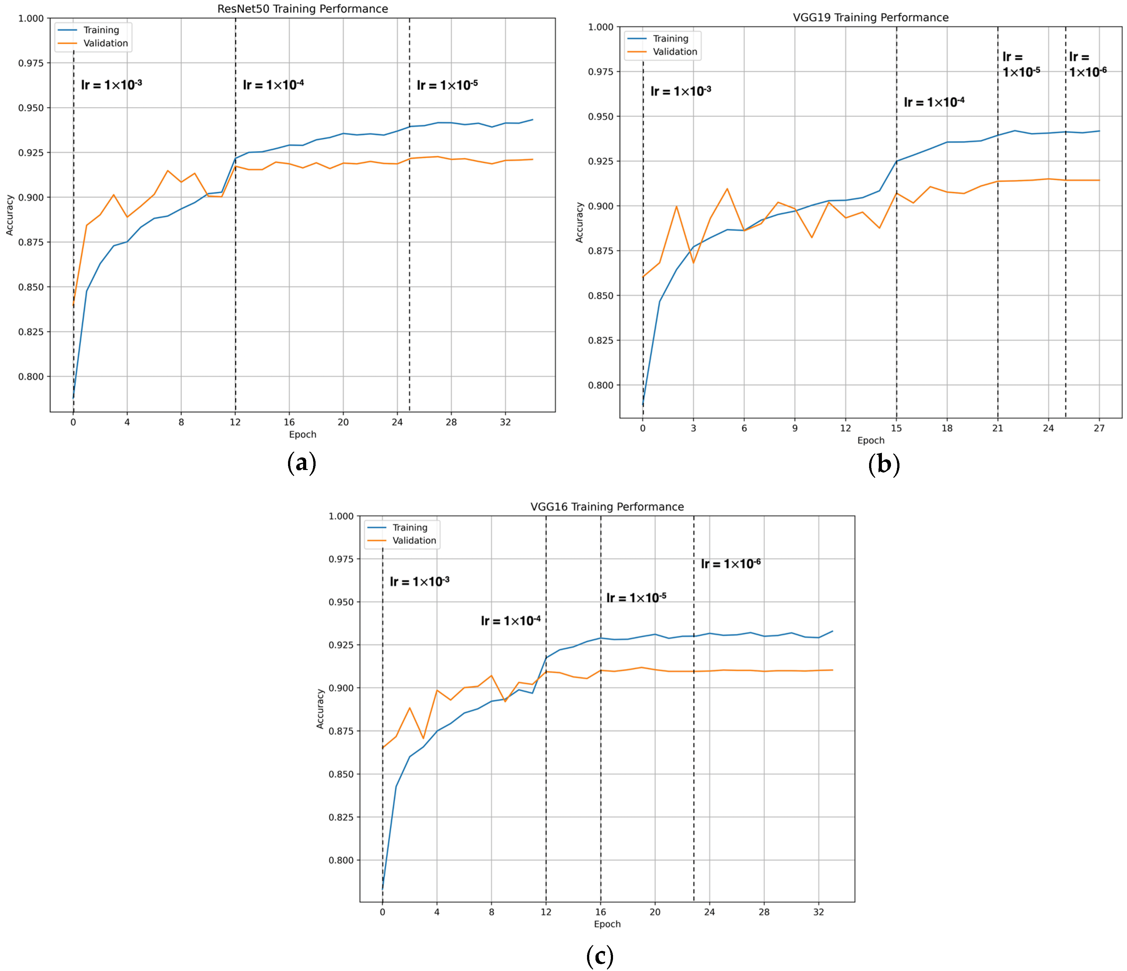
Before training, the base layers of the model (with weights trained on ImageNet) were frozen such that only the last three layers were trainable. This is common practice in deep learning, aiming to reduce computation time and preserve the essential feature extraction weights the CNN learned when trained on the ImageNet dataset. Rather than training each CNN for a fixed number of epochs, a learning rate reduction and early stopping procedure was used to strategically shift the weights towards convergence. The learning rate was first set to 0.001, and the validation loss was monitored. If the validation loss did not improve (decrease) for three epochs, known as the “patience” in Keras, the learning rate was set to 0.1 times the previous value. The minimum learning rate was set to 1 × 10⁻⁶. At any stage, the training process was terminated if there was no improvement in the validation loss for six epochs. This training procedure was performed with the Adam optimizer and with a batch size of 32. The training was performed in a Jupyter Notebook using an M1 Max Apple MacBook Pro GPU.

2.4. Grey-Level Co-Occurrence Matrix Features

A Grey-Level Co-occurrence Matrix (GLCM), first proposed by Haralick et al. (1973), is a compact method of expressing the number of times a certain pair of pixels appears along a particular direction in an image and at a particular distance apart from each other [29]. Its purpose is to allow for the computation of textural features within the image, such as its contrast and homogeneity. Given a greyscale image with 256 distinct levels of grey, its co-occurrence matrix with rows i and columns j , P i , j , will be of size 256 × 256. Assuming computation in the horizontal 0° direction and distance = 1, each value i , j in the matrix equals the number of times the pixel value pair i , j appeared in the original image horizontally and with j directly adjacent to i , as illustrated in Figure 4.
Using a GLCM, several textural image properties can be computed. A summary of the equations for calculating various image properties has been outlined in Table 2. The feature extraction from the GLCM was performed using the Sci-Kit Image Python library [30]. Each of the six GLCM image properties in Table 2 was computed. These were computed in eight directions and three distances in order to obtain as much information from each chest X-ray image as possible. This amounts to a total of 144 features (6 categories × 8 directions × 3 distances), where each “feature” is defined as a numerical value of one of the GLCM properties for a particular direction and distance.

2.5. mRMR Feature Selection

The Minimum Redundancy Maximum Relevance algorithm proposed by Ding and Peng (2005) aims to select features that are most important to classification when using traditional (non-CNN) classifiers [31,32]. Removing irrelevant features allows for quicker computation time when fitting the model to a traditional classifier and more accurate results, as there are fewer features to consider and fewer chances of model confusion [33]. Their algorithm iteratively cycles through the features and extracts the most relevant and least redundant feature at each iteration. The feature with the highest F-test statistic is selected on the first iteration. On subsequent iterations, the criterion for selection is a feature’s F-statistic divided by its average Pearson correlation to all features selected on previous iterations, as in Equation (1) below. This is known as the F-test Correlation Quotient (FCQ).
s c o r e X i = F Y , X i / ( [ 1 S X s S ρ X s , X i ] )
X i is the feature to be selected at iteration i , F Y , X i is the F-test statistic of the feature with respect to its corresponding class label Y , S is the set of previously selected features, and ρ X s , X i is the Pearson correlation coefficient of the feature to each of the previously selected features, X s .
There are many variations of this criterion depending on the specific use case. For example, if the classifier to be used on the feature set is a Random Forest Classifier, the F-test relevance criterion can be replaced with one derived from the decision tree algorithm of the classifier, known as the Gini feature importance. This substitution aims to further improve the relevance of the selected features [34]. The resulting mRMR feature selection algorithm is called the Random Forest Correlation Quotient (RFCQ).
For the present study, RFCQ was used. The number of iterations, and hence the number of features selected, was set to 160 for each feature set generated by the CNN models and 80 for the GLCM feature set. These were the values that gave the best performance when considering computation time.

2.6. Classification Process

In a secondary “training” process, a Python program was created to extract feature sets from each chest X-ray image in the COVID-QU-Ex and Mostafiz et al. training datasets. Each of the 3 trained CNNs provides 1024 features directly from their Dense-1024 layer for each image. The 144 GLCM features are also extracted in this process. Once this is complete, the features from each source are processed by the mRMR algorithm, taking only the 160 most important features from each CNN feature set and 80 from the GLCM feature set. The resulting features are then concatenated to form a final feature set of 560 features for each chest X-ray image in the training dataset.
The resulting matrix of size n i m a g e s × 560 was then passed to one of four classifiers, each of which is outlined below:

2.6.1. Random Forest Classifier (RF)

A Random Forest Classifier involves a series of individual decision tree classifiers (estimators) that individually attempt to classify randomly selected feature samples [35]. While these estimators may make errors, the majority vote of each of the many estimators gives a much more accurate prediction, leading to the success of RFs. In the current study, an RF was implemented in the Sci-Kit Learn Python library with 200 estimators.

2.6.2. Linear Discriminant Analysis (LDA)

LDA works by grouping features such that variance between classes is maximized and variance between features within a class is minimized [36]. It is commonly used when there are many data points (features) to process, such as in facial recognition or other image recognition applications that require extracting many features. In this study, it was once again implemented using Sci-Kit Learn.

2.6.3. Logistic Regression (LR)

Logistic regression builds on linear regression analysis, which analyzes the relationship between independent predictor variables and dependent outcome variables, assuming that the relationship between these variables is linear. In the case of logistic regression, the output variables are given to a sigmoid function to convert them to a probability between 0 and 1, thus allowing separation into two classes: those below 0.5 probability and those above [37]. This concept can be extended to multi-class classification, as in the Sci-Kit Learn LR algorithm implementation.

2.6.4. Artificial Neural Network (ANN)

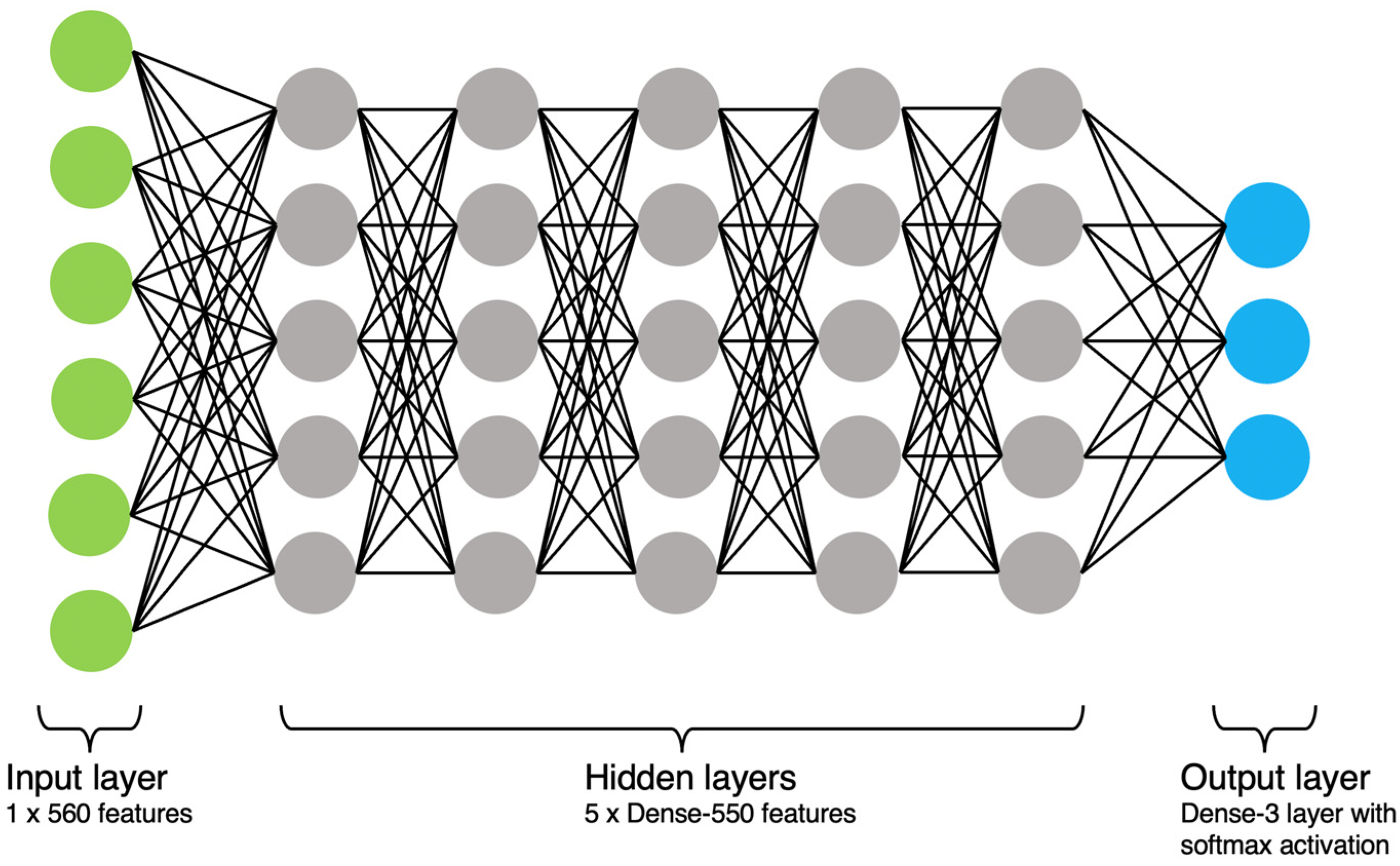
In contrast to deep neural networks (CNNs), which use 2D layers, ANNs refer to multiple 1D layers of neurons stacked on top of each other for the classification of features. They are also commonly known as multi-layer perceptrons or feed-forward neural networks. They have been successfully used in medical image classification, such as classifying CT scans containing lung nodules [38] and skin lesion malignancies [39]. For the current study, the ANN was implemented in Python’s Keras library, using an input layer with the same length as each row of features (560), 5 hidden Dense layers of 550 neurons each, and a Dense-3 layer with softmax activation at the output, as illustrated in Figure 5.
It was trained similarly to the CNNs that performed the feature extraction, utilizing learning rate reduction with four epochs of validation loss patience and early stopping after eight epochs of no improvement of the validation loss.
Once the above four classifiers had been fitted to the features from either the COVID-QU-Ex or the Mostafiz et al. training datasets, the same process was repeated to extract features from their respective test datasets. The models were then evaluated based on their predictions for each chest X-ray image.

2.7. Generalizability of Models

In order to test the generalizability performance of the models when they are trained on different datasets, four variations of dataset training and testing were performed:
(1)
Training and testing on the COVID-QU-Ex dataset.
(2)
Training and testing on the Mostafiz et al. (2022) dataset.
(3)
Training on the COVID-QU-Ex dataset and testing on Mostafiz et al. (2022) dataset.
(4)
Training on Mostafiz et al. (2022) dataset and testing on the COVID-QU-Ex dataset.
The purpose of this experiment is to investigate the influence of dataset size on the degree of overfitting and the ability of the model to extrapolate to new input images.

2.8. Classification Metrics

Several accuracy metrics were computed as outlined in Table 3, where TP/TN, FP/FN are true positive/negative and false positive/negative of class predictions respectively.

3. Results

3.1. CNN Training Results

The training and validation accuracies during the training of the three CNNs are shown in Figure 6. The benefits of using LR reduction and early stopping during network training are clear: Table 4 shows that all three CNNs had an improved test accuracy for both datasets after the modified training regime. In addition, these better test accuracies were achieved in fewer training epochs: 35, 28, and 34 for ResNet50, VGG19, and VGG16, respectively, as per Figure 6 (COVID-QU-Ex dataset).

3.2. Results for Different Classifiers

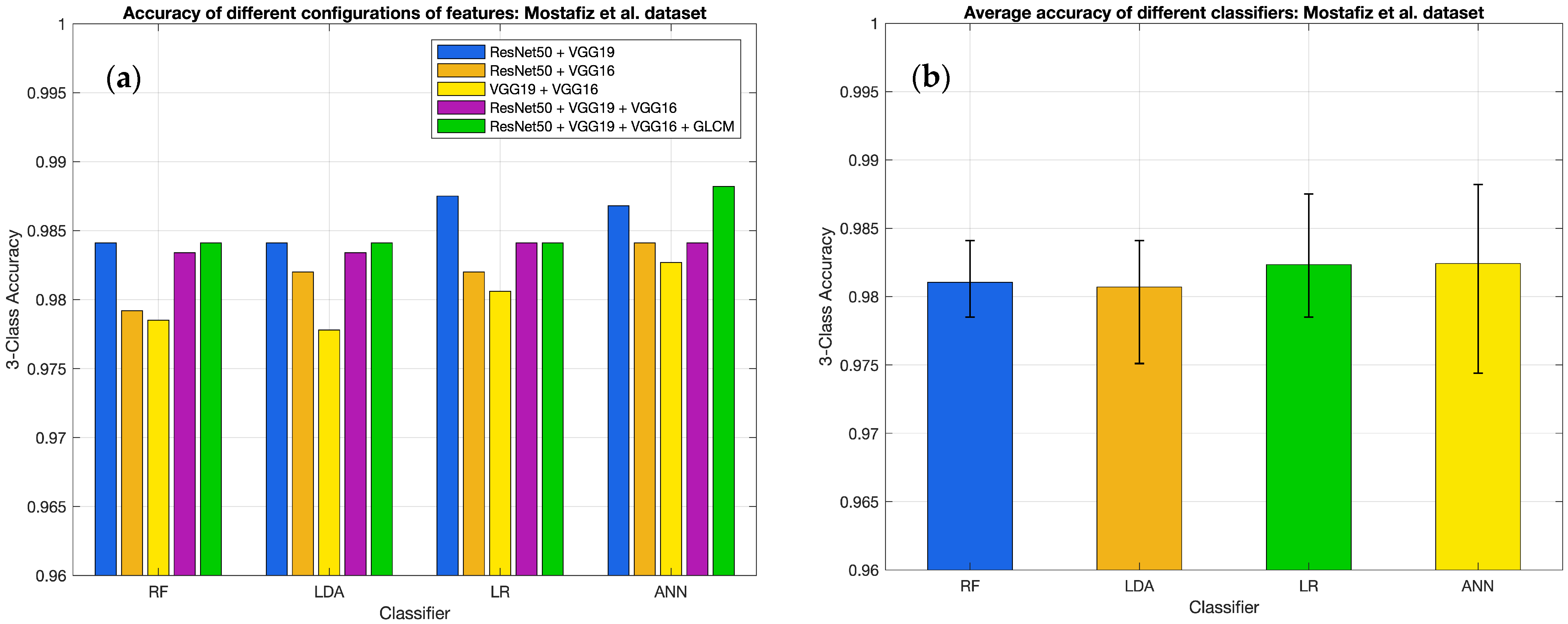
The test image classification results for each dataset are shown in Table 5 and Table 6, with graphical comparisons of the classifier performances in Figure 7 and Figure 8. Accuracy refers to the three-class accuracy for distinguishing between COVID-19, Non-COVID pneumonia, and Normal chest X-rays. The other metrics (precision, sensitivity, specificity, and F1-score) typically correspond to a single class in a dataset. However, in this case, they are macro averages of the same metrics obtained for each of the three classes.
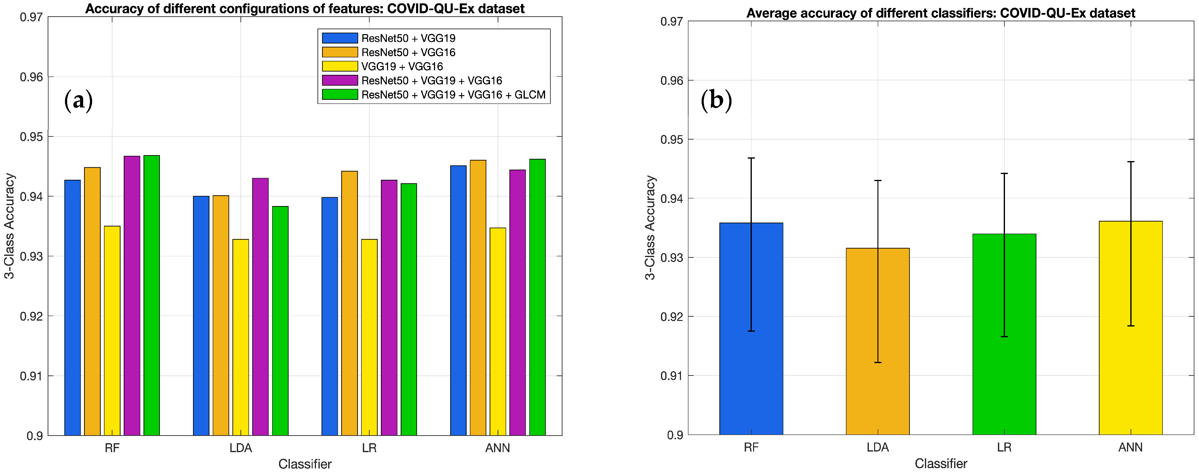
For the COVID-QU-Ex dataset, the Random Forest classifier had the best maximum performance at 94.68% accuracy on a test dataset of 6588 images. However, across all feature combinations, the ANN classifier had slightly better performance on average, at 93.61% compared to 93.58% for the RF classifier. In terms of feature combinations, the combination of VGG19 and VGG16 features consistently gave the worst performance. At the same time, the highest recorded accuracy came from the combination of all features passed to the RF classifier.
For the Mostafiz et al. dataset, RF, LDA, and LR all obtained the same accuracy when combining all features. At the same time, the ANN outperformed them, achieving a maximum accuracy of 98.82% on the test dataset of 1443 images.
On average, the best feature combination was ResNet50 with VGG19 features at 98.56% average accuracy across the different classifiers. However, combining all feature types produced a slightly lower average performance of 98.51%.

3.3. COVID-19 Detection Performance

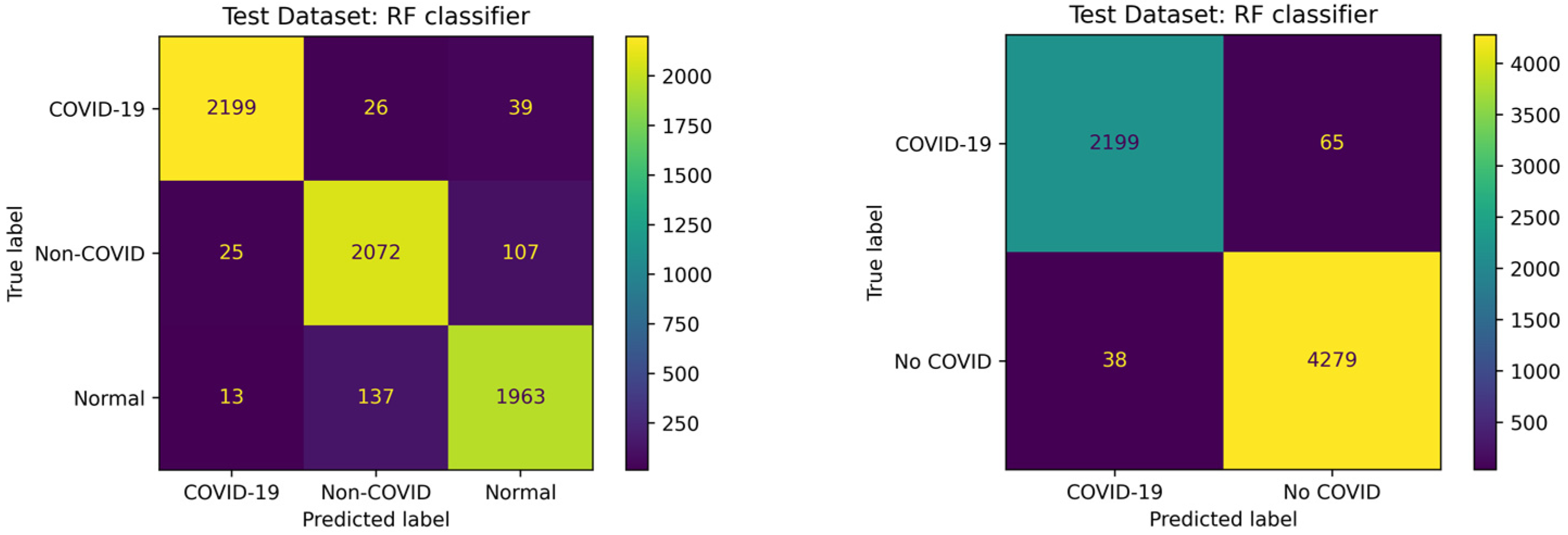
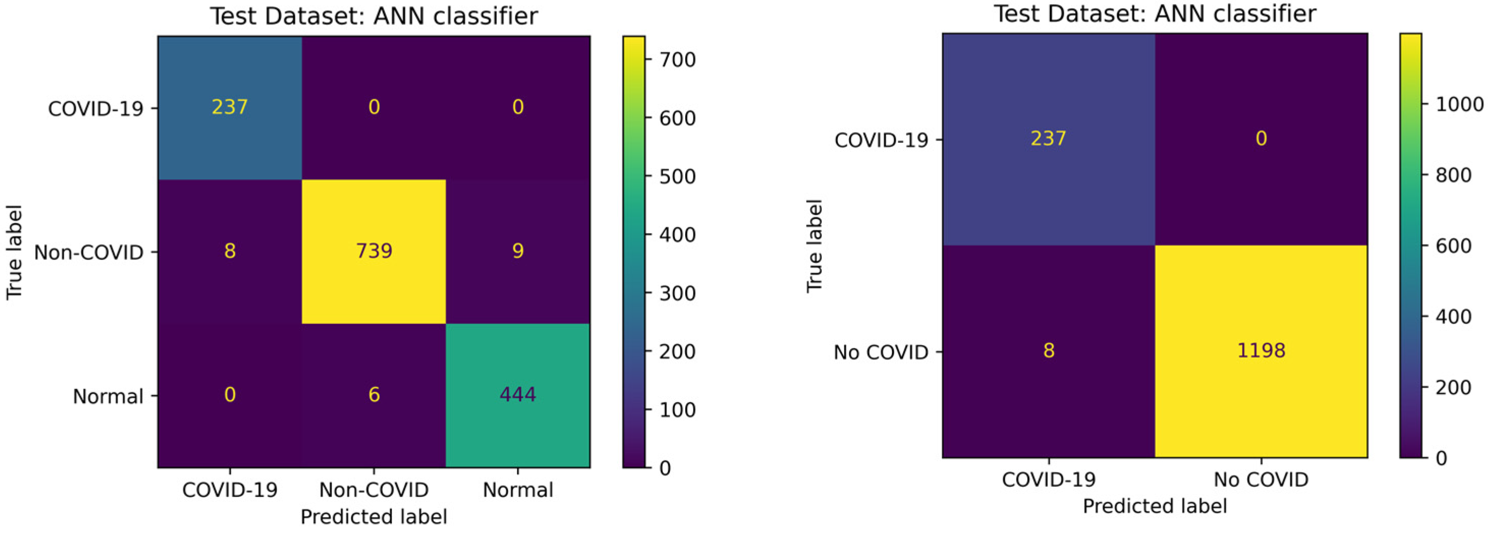
One of the primary aims of this model is to improve the performance and sensitivity of the PCR test and the general triage process for patients with COVID-19 pneumonia. Therefore, this warrants an examination of the binary classification accuracy and the specific sensitivity to COVID-19. Figure 9 and Figure 10 show the confusion matrices for a three-class classification and for a binary classification that only considers whether COVID-19 was detected or not. They correspond to the models that performed the best for each dataset: the RF classifier with all features for the larger COVID-QU-Ex dataset and the ANN classifier with all features for the smaller dataset from Mostafiz et al. Classification metrics for each are shown in Table 7.

3.4. Generalizability of Models to Unseen Data

The models clearly perform well on their respective test datasets. However, in reality, a robust model used clinically would require that it generalize well to any input chest X-ray image, not just to the test partition of the dataset it was trained on. To examine the performance on images external to the training dataset of the model (unseen/foreign data), a cross-dataset testing procedure was performed. This involved testing the model trained on the COVID-QU-Ex dataset using the dataset from Mostafiz et al. and vice versa. To ensure fairness, the COVID-QU-Ex test dataset was modified to match the number of chest X-rays in each Mostafiz et al. test dataset class. Therefore, 237 COVID-19, 756 Non-COVID, and 450 normal chest X-rays were randomly selected from the COVID-QU-Ex test dataset. All four types of end classifiers were examined, with the results shown in Figure 11a,b.
It is apparent in Figure 11a that, other than for the LDA classifier, the generalization of the model trained on the larger dataset is excellent, achieving accuracies even higher than for its own test dataset. On the other hand, evidently, the LDA classifier is severely prone to overfitting and does not generalize well to new data. This was also clear in Figure 11b for the model trained on the smaller Mostafiz et al. dataset and tested on data from COVID-QU-Ex. In contrast to Figure 11a, however, Figure 11b shows that the other classifiers also did not generalize well for this dataset, achieving only around 70% accuracy for RF, LR, and ANN. This points to the issue of the CNNs poorly extracting features from unseen images. To summarize, the results reaffirm that training on a larger (>20,000 image) dataset allows the end model to better generalize to new data than training on a smaller (~4000 image) dataset.

4. Discussion

The results of training the CNNs show that improving their test dataset accuracy is possible by strategically lowering the learning rate and using early stopping. Learning rate reduction is also known as learning rate scheduling and has a significant influence on gradient descent in the training process. Having a relatively large learning rate when training begins allows a rough and rapid estimation of the model minimum loss, with further decreases in learning rate tuning the model weights with finer and finer steps until the loss converges to a global minimum [40]. This is analogous to first using a coarse focus followed by a fine focus to visualize an object under a microscope with high magnification. Continuously using the same high learning rate throughout the training process makes it far more difficult for the weights to converge to their ideal values. This is because the weights experience larger shifts in their values, similar to relying solely on coarse focus when using a microscope. This can cause the model to converge at local minima instead [41]. Conversely, using only a low learning rate will substantially increase the computation time and likewise may get stuck at local minima. Using strategic learning rate reduction, test accuracies were improved by 1.53% on average and required fewer training epochs, reducing the computational load.
The classification results exemplify the benefits of ensemble techniques in medical image classification for improving the accuracies obtained via CNN classification. For the COVID-QU-Ex dataset, the mean accuracy for classifying features from individual CNNs was 92.36% for the RF classifier. However, combining features from each CNN, GLCM features, and classification using traditional machine learning classifiers yielded a substantial improvement of a maximum three-class accuracy of 94.68% with the RF classifier. The benefits resulting from such ensemble CNN approaches have been documented in other studies. Togacar et al. (2020) used a similar CNN feature concatenation approach for pneumonia detection in chest X-rays and attained a binary accuracy about 2.7% higher than for their individual CNNs [10]. The approach appears to be able to be extended to other specific diseases, such as tuberculosis detection, as demonstrated by Hooda et al. (2019), who saw a 5.5% increase in TB detection accuracy when combining the features extracted by AlexNet, GoogleNet, and ResNet34 [42].
The results in Figure 9 and Figure 10 show that, for both datasets, any confusion mostly resided in distinguishing between Non-COVID pneumonia and Normal chest X-rays and not significantly between either of these and the COVID-19 chest X-rays. This means that the binary classification (COVID-19 detected/not detected) was excellent in both cases, with an accuracy of 98.43% for the larger COVID-QU-Ex dataset and 99.86% for the smaller Mostafiz et al. dataset. The binary COVID-19 detection accuracy was, in fact, slightly improved over that obtained by Mostafiz et al., who achieved 99.45% [6]. The sensitivity to COVID-19 was similarly high, at 97.13% for the large dataset and 100% for the smaller dataset. Both instances perform better than a PCR, which is, on average, about 90.7% sensitive to COVID-19 [1]. Figure 11a shows that as long as the model is trained on sufficient data, these accurate metrics can be maintained when applying the model to new data, allowing it to be adequately used as a clinical diagnostic tool.
There have been numerous research articles presenting COVID-19 chest X-ray classification models trained on small datasets of only a few hundred to a few thousand images, some of which document very high (>98) accuracies [3,4,5,6,7,8,9]. The significance of the present study is that it shows that high accuracy on small datasets does not mean that the model generalizes well and is robust to other datasets, which is the overall aim of developing such models in the first place. The generalizability of machine learning models is especially critical in a clinical environment, where, between hospitals, there may be differences in medical image acquisition systems, patient demographics, and professional training [43]. It is well understood that increasing dataset size improves the ability of CNNs and other machine learning classifiers to fit input data and reduce dataset overfitting [44,45]. The cleaned COVID-QU-Ex dataset used for training contained 11,380 chest X-rays with COVID-19, 11,048 with Non-COVID pneumonia, and 10,529 with no condition. Due to the large number and consequent variety of images, the CNNs learned more general features during training. Therefore, they could generalize very well when exposed to foreign chest X-ray images from Mostafiz et al., obtaining an average of 96.7% accuracy across different classifiers (excluding the LDA classifier outlier). On the other hand, the Mostafiz et al. dataset contained only 790 cases of COVID-19, 2519 Non-COVID pneumonia, and 1500 cases of no condition. Consequently, the CNNs learned to extract features specific to this dataset very accurately but exhibited poor generalization when given the COVID-QU-Ex images. The models obtained an average accuracy of 70.57% across the different classifiers (excluding the LDA classifier outlier). The consequence of this result is that training dataset size has a direct impact on the accuracy of predictions and must be considered when attempting to develop clinically relevant and robust automatic classification models.
For both cross-dataset tests, the LDA classifier performed poorly, clearly a sign of overfitting the image features from the dataset on which it was trained. Unlike the similar Principle Component Analysis (PCA), where insignificant features are ignored, they are included in the LDA calculation, causing the model to fit specific features rather than general ones [36,46]. This may make this particular classifier unsuitable in scenarios such as medical image classification, where there are typically a high number of input features and differences in X-ray acquisition systems that can introduce variability in the images. On the other hand, RF, LR, and ANN classifiers appear to generalize well to new features. In particular, the COVID-QU-Ex-trained ANN classifier achieved an outlier of 98.34% accuracy on the unseen Mostafiz et al. dataset. This suggests its superior use when classifying new chest X-ray images.
One limitation of the current study is the lack of labeled image data to discern between mild, moderate, and severe cases of COVID-19 or other forms of pneumonia. Naturally, each of these cases requires different levels of treatment. A clinically relevant automated diagnosis tool would ideally offer a prediction for the severity of the disease and the disease type to allow clinicians to make better treatment decisions. Future work addressing this need is therefore greatly encouraged.

5. Conclusions

This study examined several medical image deep learning techniques and elucidated the benefits of combining CNNs for improved classification performance. It was found that using learning rate reduction/scheduling can reduce CNN training time while substantially improving their test dataset classification performance. Similarly, mRMR feature selection reduces the computation time for fitting features to other classifiers while preserving relevant image information. The maximum classification accuracy for the COVID-QU-Ex dataset was achieved when extracted features from all of ResNet50, VGG19, VGG16, and GLCM were combined at 94.68% with the Random Forest classifier. Detection accuracy and sensitivity to COVID-19 were very high, at 98.43% and 97.13%, respectively. These were even higher for the Mostafiz et al. dataset, with 99.86% binary accuracy and 100% sensitivity when the ANN classifier was used. However, it was found that the small number of images caused the model to overfit the data, leading to poor generalization for all classifier types. Therefore, it is recommended to prioritize training with large datasets when creating new or improved COVID-19 or pneumonia classification models. It is also recommended to avoid using LDA classifiers when using large numbers of input features due to their poor generalizability in medical image classification.

Author Contributions

D.K. contributed to the programmatic implementation of machine learning models for the image classification application presented and article writing; S.C. contributed to advice, suggestions, and article editing. All authors have read and agreed to the published version of the manuscript.

Funding

This research received no external funding.

Data Availability Statement

All generated data are presented in the article body.

Acknowledgments

Domantas Kuzinkovas acknowledges the support of the Vacation Research Internship Winter Program Scholarship at the Faculty of Engineering, The University of Sydney, Australia.

Conflicts of Interest

The authors declare no conflict of interest.

References

  1. Kanji, J.N.; Zelyas, N.; MacDonald, C.; Pabbaraju, K.; Khan, M.N.; Prasad, A.; Hu, J.; Diggle, M.; Berenger, B.M.; Tipples, G. False Negative Rate of COVID-19 PCR Testing: A Discordant Testing Analysis. Virol. J. 2021, 18, 13. [Google Scholar] [CrossRef] [PubMed]
  2. Rodriguez-Ruiz, A.; Lång, K.; Gubern-Merida, A.; Broeders, M.; Gennaro, G.; Clauser, P.; Helbich, T.H.; Chevalier, M.; Tan, T.; Mertelmeier, T.; et al. Stand-Alone Artificial Intelligence for Breast Cancer Detection in Mammography: Comparison with 101 Radiologists. JNCI J. Natl. Cancer Inst. 2019, 111, 916–922. [Google Scholar] [CrossRef] [PubMed]
  3. Wang, L.; Lin, Z.Q.; Wong, A. COVID-Net: A Tailored Deep Convolutional Neural Network Design for Detection of COVID-19 Cases from Chest X-Ray Images. Sci. Rep. 2020, 10, 19549. [Google Scholar] [CrossRef] [PubMed]
  4. Sufian, A.; Ghosh, A.; Sadiq, A.S.; Smarandache, F. A Survey on Deep Transfer Learning to Edge Computing for Mitigating the COVID-19 Pandemic. J. Syst. Archit. 2020, 108, 101830. [Google Scholar] [CrossRef]
  5. Zouch, W.; Sagga, D.; Echtioui, A.; Khemakhem, R.; Ghorbel, M.; Mhiri, C.; Hamida, A.B. Detection of COVID-19 from CT and Chest X-Ray Images Using Deep Learning Models. Ann. Biomed. Eng. 2022, 50, 825–835. [Google Scholar] [CrossRef] [PubMed]
  6. Mostafiz, R.; Uddin, M.S.; Alam, N.-A.; Reza, M.; Rahman, M.M. Covid-19 Detection in Chest X-Ray through Random Forest Classifier Using a Hybridization of Deep CNN and DWT Optimized Features. J. King Saud Univ. Comput. Inf. Sci. 2022, 34, 3226–3235. [Google Scholar] [CrossRef]
  7. Sethy, P.K.; Behera, S.K.; Ratha, P.K.; Biswas, P. Detection of Coronavirus Disease (COVID-19) Based on Deep Features and Support Vector Machine. Int. J. Math. Eng. Manag. Sci. 2020, 5, 643–651. [Google Scholar] [CrossRef]
  8. Saha, P.; Sadi, M.S.; Islam, M. EMCNet: Automated COVID-19 Diagnosis from X-Ray Images Using Convolutional Neural Network and Ensemble of Machine Learning Classifiers. Inform. Med. Unlocked 2021, 22, 100505. [Google Scholar] [CrossRef]
  9. Karim, A.M.; Kaya, H.; Alcan, V.; Sen, B.; Hadimlioglu, I.A. New Optimized Deep Learning Application for COVID-19 Detection in Chest X-Ray Images. Symmetry 2022, 14, 1003. [Google Scholar] [CrossRef]
  10. Toğaçar, M.; Ergen, B.; Cömert, Z.; Özyurt, F. A Deep Feature Learning Model for Pneumonia Detection Applying a Combination of MRMR Feature Selection and Machine Learning Models. IRBM 2020, 41, 212–222. [Google Scholar] [CrossRef]
  11. Tahir, A.M.; Chowdhury, M.; Qiblawey, Y.; Khandakar, A.; Rahman, T.; Kiranyaz, S.; Khurshid, U.; Ibtehaz, N.; Mahmud, S.; Ezeddin, M. COVID-QU-Ex Dataset; Kaggle: San Francisco, CA, USA, 2021. [Google Scholar] [CrossRef]
  12. Chowdhury, M.E.H.; Rahman, T.; Khandakar, A.; Mazhar, R.; Kadir, M.A.; Mahbub, Z.B.; Islam, K.R.; Khan, M.S.; Iqbal, A.; Emadi, N.A.; et al. Can AI Help in Screening Viral and COVID-19 Pneumonia? IEEE Access 2020, 8, 132665–132676. [Google Scholar] [CrossRef]
  13. Rahman, T.; Khandakar, A.; Qiblawey, Y.; Tahir, A.; Kiranyaz, S.; Abul Kashem, S.B.; Islam, M.T.; Al Maadeed, S.; Zughaier, S.M.; Khan, M.S.; et al. Exploring the Effect of Image Enhancement Techniques on COVID-19 Detection Using Chest X-Ray Images. Comput. Biol. Med. 2021, 132, 104319. [Google Scholar] [CrossRef] [PubMed]
  14. De la Iglesia Vayá, M.; Saborit-Torres, J.M.; Montell Serrano, J.A.; Oliver-Garcia, E.; Pertusa, A.; Bustos, A.; Cazorla, M.; Galant, J.; Barber, X.; Orozco-Beltrán, D.; et al. BIMCV COVID-19+: A Large Annotated Dataset of RX and CT Images from COVID-19 Patients. arXiv 2021, arXiv:2006.01174. [Google Scholar] [CrossRef]
  15. Covid-19-Image-Repository/Png at Master Ml-Workgroup/COVID-19-Image-Repository. Available online: https://github.com/ml-workgroup/covid-19-image-repository (accessed on 22 June 2023).
  16. SIRM—Società Italiana di Radiologia Medica e Interventistica. 2022. Available online: https://sirm.org/ (accessed on 22 June 2023).
  17. Eurorad.Org. Available online: https://www.eurorad.org/homepage (accessed on 22 June 2023).
  18. COVID-19 Chest X-ray Image Repository. 2020. Available online: https://figshare.com/articles/dataset/COVID-19_Chest_X-Ray_Image_Repository/12580328/3 (accessed on 22 June 2023).
  19. Haghanifar, A. COVID-CXNet 2023. Available online: https://github.com/armiro/COVID-CXNet (accessed on 22 June 2023).
  20. RSNA Pneumonia Detection Challenge. Available online: https://kaggle.com/competitions/rsna-pneumonia-detection-challenge (accessed on 22 June 2023).
  21. Chest X-ray Images (Pneumonia). Available online: https://www.kaggle.com/datasets/paultimothymooney/chest-xray-pneumonia (accessed on 22 June 2023).
  22. Mostafiz, R. Chest-X-ray. GitHub. 2020. Available online: https://github.com/rafid909/Chest-X-ray (accessed on 22 June 2023).
  23. Cohen, J.P.; Morrison, P.; Dao, L. COVID-19 Image Data Collection. arXiv 2020, arXiv:2003.11597. [Google Scholar] [CrossRef]
  24. Dadario, A.M.V. COVID-19 X rays; Kaggle: San Francisco, CA, USA, 2020. [Google Scholar] [CrossRef]
  25. Kermany, D.; Zhang, K.; Goldbaum, M. Labeled Optical Coherence Tomography (OCT) and Chest X-ray Images for Classification; Mendeley Data, Version 2; Elsevier inc.: Amsterdam, The Netherlands, 2018. [Google Scholar] [CrossRef]
  26. Smazzanti. mRMR Python Package. GitHub. 2022. Available online: https://github.com/smazzanti/mrmr (accessed on 4 January 2023).
  27. Deng, J.; Dong, W.; Socher, R.; Li, L.-J.; Li, K.; Li, F.-F. ImageNet: A Large-Scale Hierarchical Image Database. In Proceedings of the 2009 IEEE Conference on Computer Vision and Pattern Recognition, Miami, FL, USA, 20–25 June 2009; pp. 248–255. [Google Scholar]
  28. Chollet, F. Keras: Deep Learning for Humans. Available online: https://keras.io/ (accessed on 4 January 2023).
  29. Haralick, R.M.; Shanmugam, K.; Dinstein, I. Textural Features for Image Classification. IEEE Trans. Syst. Man Cybern. 1973, SMC-3, 610–621. [Google Scholar] [CrossRef] [Green Version]
  30. Pedregosa, F.; Varoquaux, G.; Gramfort, A.; Michel, V.; Thirion, B.; Grisel, O.; Blondel, M.; Prettenhofer, P.; Weiss, R.; Dubourg, V.; et al. Scikit-Learn: Machine Learning in Python. J. Mach. Learn. Res. 2011, 12, 2825–2830. [Google Scholar]
  31. Ding, C.; Peng, H. Minimum Redundancy Feature Selection from Microarray Gene Expression Data. J. Bioinform. Comput. Biol. 2005, 3, 185–205. [Google Scholar] [CrossRef]
  32. Peng, H.; Long, F.; Ding, C. Feature Selection Based on Mutual Information Criteria of Max-Dependency, Max-Relevance, and Min-Redundancy. IEEE Trans. Pattern Anal. Mach. Intell. 2005, 27, 1226–1238. [Google Scholar] [CrossRef]
  33. Zhao, Z.; Anand, R.; Wang, M. Maximum Relevance and Minimum Redundancy Feature Selection Methods for a Marketing Machine Learning Platform. In Proceedings of the 2019 IEEE International Conference on Data Science and Advanced Analytics (DSAA), Washington, DC, USA, 5–8 October 2019; pp. 442–452. [Google Scholar] [CrossRef] [Green Version]
  34. Menze, B.H.; Kelm, B.M.; Masuch, R.; Himmelreich, U.; Bachert, P.; Petrich, W.; Hamprecht, F.A. A Comparison of Random Forest and Its Gini Importance with Standard Chemometric Methods for the Feature Selection and Classification of Spectral Data. BMC Bioinform. 2009, 10, 213. [Google Scholar] [CrossRef] [Green Version]
  35. Fawagreh, K.; Gaber, M.M.; Elyan, E. Random Forests: From Early Developments to Recent Advancements. Syst. Sci. Control. Eng. 2014, 2, 602–609. [Google Scholar] [CrossRef] [Green Version]
  36. Liu, R.; Gillies, D.F. Overfitting in Linear Feature Extraction for Classification of High-Dimensional Image Data. Pattern Recognit. 2016, 53, 73–86. [Google Scholar] [CrossRef] [Green Version]
  37. Schober, P.; Vetter, T.R. Logistic Regression in Medical Research. Obstet. Anesthesia Dig. 2021, 132, 365–366. [Google Scholar] [CrossRef] [PubMed]
  38. Upadhyay, S.; Tanwar, P.S. Classification of Benign-Malignant Pulmonary Lung Nodules Using Ensemble Learning Classifiers. In Proceedings of the 2021 6th International Conference on Communication and Electronics Systems (ICCES), Coimbatore, India, 8–10 July 2021; pp. 1–8. [Google Scholar]
  39. Majumder, S.; Ullah, M.A. Feature Extraction from Dermoscopy Images for an Effective Diagnosis of Melanoma Skin Cancer. In Proceedings of the 2018 10th International Conference on Electrical and Computer Engineering (ICECE), Dhaka, Bangladesh, 20–22 December 2018; pp. 185–188. [Google Scholar]
  40. Senior, A.; Heigold, G.; Ranzato, M.; Yang, K. An Empirical Study of Learning Rates in Deep Neural Networks for Speech Recognition. In Proceedings of the 2013 IEEE International Conference on Acoustics, Speech and Signal Processing, Vancouver, BC, Canada, 26–31 May 2013; pp. 6724–6728. [Google Scholar]
  41. Johny, A.; Madhusoodanan, K.N. Dynamic Learning Rate in Deep CNN Model for Metastasis Detection and Classification of Histopathology Images. Comput. Math. Methods Med. 2021, 2021, e5557168. [Google Scholar] [CrossRef]
  42. Hooda, R.; Mittal, A.; Sofat, S. Automated TB Classification Using Ensemble of Deep Architectures. Multimed. Tools Appl. 2019, 78, 31515–31532. [Google Scholar] [CrossRef]
  43. Futoma, J.; Simons, M.; Panch, T.; Doshi-Velez, F.; Celi, L.A. The Myth of Generalisability in Clinical Research and Machine Learning in Health Care. Lancet Digit. Health 2020, 2, e489–e492. [Google Scholar] [CrossRef]
  44. Prusa, J.; Khoshgoftaar, T.M.; Seliya, N. The Effect of Dataset Size on Training Tweet Sentiment Classifiers. In Proceedings of the 2015 IEEE 14th International Conference on Machine Learning and Applications (ICMLA), Miami, FL, USA, 9–11 December 2015; pp. 96–102. [Google Scholar]
  45. Althnian, A.; AlSaeed, D.; Al-Baity, H.; Samha, A.; Dris, A.B.; Alzakari, N.; Abou Elwafa, A.; Kurdi, H. Impact of Dataset Size on Classification Performance: An Empirical Evaluation in the Medical Domain. Appl. Sci. 2021, 11, 796. [Google Scholar] [CrossRef]
  46. Luo, D.; Ding, C.; Huang, H. Linear Discriminant Analysis: New Formulations and Overfit Analysis. Proc. AAAI Conf. Artif. Intell. 2011, 25, 417–422. [Google Scholar] [CrossRef]
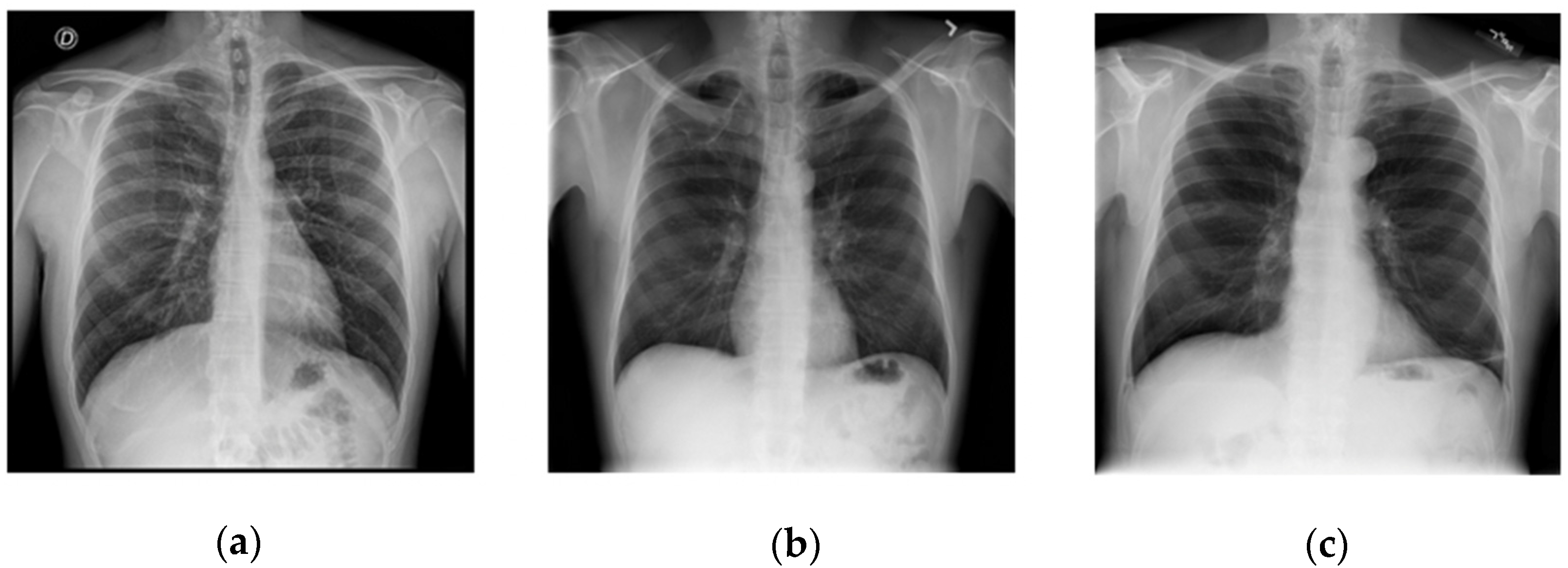
Figure 1. Examples of (a) COVID-19, (b) Non-COVID Pneumonia, and (c) Normal chest X-ray images from the COVID-QU-Ex dataset [11].
Information 14 00370 g001
Figure 2. Proposed ensemble CNN, GLCM, and traditional classifier chest X-ray classification model.
Information 14 00370 g002
Figure 3. Schematic of how the three CNNs were modified to classify chest X-rays during the training process. The CNNs were then used for feature extraction purposes, whereby the Dense-3 layer was removed and the final Dense-1024 layer (without dropout) was used to provide 1024 features for classification.
Information 14 00370 g003
Figure 4. GLCM transformation on 3 × 3 arrangement of pixels with values 0–2. Performed at 0 ° angle and pixel distance 1.
Information 14 00370 g004
Figure 5. Structure of custom ANN classifier.
Information 14 00370 g005
Figure 6. Training curves on the COVID-QU-Ex dataset for (a) ResNet50, (b) VGG19, and (c) VGG16. Vertical dashed lines show when a new learning rate (lr) was applied by the training algorithm. Blue curves show training accuracy, and orange curves show validation accuracy.
Information 14 00370 g006
Figure 7. COVID-QU-Ex test dataset classification accuracies for different classifier configurations. (a) Comparison of accuracies resulting from different feature combinations (features from individual CNNs are not shown for clarity). (b) Average classification accuracy (including individual CNN features) for each type of classifier. Error bars show a range of values.
Information 14 00370 g007
Figure 8. Mostafiz et al. test dataset classification accuracies for different classifier configurations. (a) Comparison of accuracies resulting from different feature combinations (features from individual CNNs are not shown for clarity). (b) Average classification accuracy (including individual CNN features) for each type of classifier. Error bars show a range of values.
Information 14 00370 g008
Figure 9. Three-Class (left) and binary (right) classification confusion matrices for the highest performing model in COVID-QU-Ex dataset testing: RF classifier with all features.
Information 14 00370 g009
Figure 10. Three-Class (left) and binary (right) classification confusion matrices for the highest performing model in Mostafiz et al. dataset testing: ANN classifier with all features.
Information 14 00370 g010
Figure 11. (a) Results of training the model on a large dataset and testing it on an unseen dataset. (b) Results of training the model on a small dataset and testing it on an unseen dataset.
Information 14 00370 g011
Table 1. Dataset sample numbers for COVID-QU-Ex and Mostafiz et al. (2022) datasets.
Dataset and ClassesTrainValTestTotal
COVID-QU-Ex [11]
COVID-1972901826226411,380
Non-COVID Pneumonia70821762220411,048
Normal67301686211310,529
Total21,1025274658132,957
Mostafiz et al. (2022) [6,22]
COVID-19442111237790
Non-COVID Pneumonia14103537562519
Normal8402104501500
Total269267414434809
Table 2. GLCM properties and their definitions.
GLCM PropertyMeaningEquation
ContrastMeasure of local variations in pixel values. i , j = 0 N l e v e l s 1 P i , j i j 2
DissimilarityMeasure of absolute difference in pixel intensities. i , j = 0 N l e v e l s 1 P i , j i j
HomogeneityMeasure of the local homogeneity of pixels in the image. i , j = 0 N l e v e l s 1 P i , j 1 + i j 2
ASMMeasure of overall homogeneity of pixels in the image. i , j = 0 N l e v e l s 1 P i , j 2
EnergySquare root of ASM. A S M
CorrelationMeasure of how linearly correlated pairs of pixels are over the whole image. i , j = 0 N l e v e l s 1 P i , j i μ i j μ j σ i σ j
Note: P i , j is a value at row i and column j in the GLCM; N l e v e l s is the number of grey levels, μ i and μ j are the mean of the current column and current row in the GLCM, respectively; and σ i and σ j are the standard deviations of the current column and current row, respectively.
Table 3. Classification performance metrics.
MetricEquation
Accuracy T P + T N T P + T N + F P + F N
Precision T P T P + F P
Sensitivity T P T P + F N
Specificity T N T N + F P
F1-score 2 T P 2 T P + F P + F N
Table 4. Three-Class CNN Test Accuracy with and without LR reduction and early stopping.
COVID-QU-Ex DatasetMostafiz et al. Dataset
CNNSimple Training (40 Epochs)LR Reduction + Early StoppingSimple Training (40 Epochs)LR Reduction + Early Stopping
ResNet500.91840.93370.97850.9806
VGG190.91230.91890.96740.9709
VGG160.89910. 92310.97290.9757
Table 5. Classification metrics for different combinations of input features: COVID-QU-Ex dataset. Best values for each metric are shown in bold.
Classifier and MetricsResNet50VGG19VGG16ResNet50
+
VGG19
ResNet50 +
VGG16
VGG19
+
VGG16
ResNet50 + VGG19 + VGG16ResNet50 + VGG19 + VGG16 + GLCM
RF
Accuracy0.93070.91750.92250.94270.94480.93500.94670.9468
Precision0.93040.91720.92210.94250.94450.93480.94630.9465
Sensitivity0.93020.91700.92210.94220.94450.93460.94610.9463
Specificity 0.96550.95890.96140.97150.97260.96760.97350.9735
F1-score0.93030.91710.92210.94230.94450.93460.94620.9464
LDA
Accuracy0.92680.91220.91930.94000.94010.93280.94300.9383
Precision0.92650.91190.91890.93970.93980.93270.94270.9386
Sensitivity0.92640.91170.91890.93960.93970.93250.94260.9379
Specificity 0.96350.95630.95980.97010.97020.96660.97160.9693
F1-score0.92640.91180.91890.93960.93970.93250.94260.9380
LR
Accuracy0.93040.91660.92310.93980.94420.93280.94270.9421
Precision0.93010.91650.92270.93950.94370.93270.94240.9418
Sensitivity0.93000.91630.92270.93930.94370.93250.94230.9416
Specificity 0.96540.95850.96170.97010.97220.96660.97150.9712
F1-score0.93000.91630.92270.93940.94370.93250.94230.9417
ANN
Accuracy0.92990.91840.92430.94510.94600.93470.94440.9462
Precision0.92980.91830.92400.94480.94710.93470.94430.9460
Sensitivity0.92950.91780.92410.94470.94720.93430.94400.9457
Specificity 0.96510.95940.96230.97270.97390.96750.97230.9732
F1-score0.92950.91800.92390.94470.94710.93440.94400.9458
Table 6. Classification metrics for different combinations of input features: Mostafiz et al. dataset. Best values for each metric are shown in bold.
Classifier and MetricsResNet50VGG19VGG16ResNet50
+
VGG19
ResNet50 +
VGG16
VGG19
+
VGG16
ResNet50 + VGG19 + VGG16ResNet50 + VGG19 + VGG16 + GLCM
RF
Accuracy0.98130.97850.97920.98410.97920.97850.98340.9841
Precision0.97980.97940.98010.98270.97700.97920.98200.9827
Sensitivity0.98440.98140.97860.98620.98310.98170.98580.9862
Specificity 0.98970.98790.98830.99110.98880.98810.99070.9911
F1-score0.98210.98040.97940.98440.98000.98040.98380.9844
LDA
Accuracy0.98270.97640.97510.98410.98200.97780.98340.9841
Precision0.98130.97410.97790.98250.98050.97600.98200.9831
Sensitivity0.98600.98040.97620.98720.98550.98160.98640.9872
Specificity 0.99040.98740.98480.99120.99010.98820.99070.9912
F1-score0.98360.97720.97700.98480.98300.97870.98420.9851
LR
Accuracy0.98200.97850.97990.98750.98200.98060.98410.9841
Precision0.98050.97920.98290.98770.97990.98100.98360.9836
Sensitivity0.98550.98210.98020.98900.98700.98270.98810.9881
Specificity 0.99010.98810.98750.99290.99080.98920.99150.9915
F1-score0.98300.98060.98150.98840.98340.98190.98580.9858
ANN
Accuracy0.98060.97850.97440.98680.98410.98270.98410.9882
Precision0.97870.97770.97190.98540.98390.98340.98390.9872
Sensitivity0.98370.98320.97930.98950.98560.98490.98610.9916
Specificity 0.98930.98910.98700.99280.99070.99050.99140.9940
F1-score0.98120.98020.97530.98750.98470.98410.98500.9893
Table 7. Best performing model COVID-19 metrics for each dataset.
MetricCOVID-QU-Ex Dataset with RFMostafiz et al. Dataset with ANN
Three-Class Accuracy0.94680.9882
Binary Accuracy0.98430.9986
Sensitivity to COVID-190.97131.0
Disclaimer/Publisher’s Note: The statements, opinions and data contained in all publications are solely those of the individual author(s) and contributor(s) and not of MDPI and/or the editor(s). MDPI and/or the editor(s) disclaim responsibility for any injury to people or property resulting from any ideas, methods, instructions or products referred to in the content.