Article

Regularized Mislevy-Wu Model for Handling Nonignorable Missing Item Responses

by
Alexander Robitzsch
1,2
1
Department of Educational Measurement and Data Science, IPN—Leibniz Institute for Science and Mathematics Education, Olshausenstraße 62, 24118 Kiel, Germany
2
Centre for International Student Assessment (ZIB), Olshausenstraße 62, 24118 Kiel, Germany
Information 2023, 14(7), 368; https://doi.org/10.3390/info14070368
Submission received: 17 May 2023 / Revised: 21 June 2023 / Accepted: 26 June 2023 / Published: 28 June 2023
(This article belongs to the Topic Soft Computing)

Abstract

:
Missing item responses are frequently found in educational large-scale assessment studies. In this article, the Mislevy-Wu item response model is applied for handling nonignorable missing item responses. This model allows that the missingness of an item depends on the item itself and a further latent variable. However, with low to moderate amounts of missing item responses, model parameters for the missingness mechanism are difficult to estimate. Hence, regularized estimation using a fused ridge penalty is applied to the Mislevy-Wu model to stabilize estimation. The fused ridge penalty function is separately defined for multiple-choice and constructed response items because previous research indicated that the missingness mechanisms strongly differed for the two item types. In a simulation study, it turned out that regularized estimation improves the stability of item parameter estimation. The method is also illustrated using international data from the progress in international reading literacy study (PIRLS) 2011 data.

1. Introduction

In educational large-scale assessment (LSA) studies [1,2], such as the progress in international reading literacy study (PIRLS; [3]), the trends in international mathematics and science study (TIMSS; [4]), or the programme for international student assessment (PISA; [5]), students’ abilities are assessed using cognitive test items. Often, however, students do not respond to specific items leading to missing item responses [6]. It is not obvious how item nonresponse  [7] should be treated in the computation of values of abilities (i.e., values of the latent trait) in item response theory (IRT) models  [8,9,10] that are used as scaling models.
Researchers frequently argue for applying complex IRT models that model missing item responses in order to avoid biased item parameters [6,11]. If students omit items, the most obvious option would be treating them as either wrong or missing, which effectively means removing them from the estimation. In the latter case, missing item responses are simply ignored. Slightly more complex treatments assume that missing item responses can be ignored when conditioning on further latent variables (i.e., latent ignorability; [12]). However, it has been shown that these kinds of models do not adequately fit typical LSA datasets [13]. Recently, the Mislevy-Wu (MW) model received some attention  [7,13,14,15,16] that relaxes the strict assumption that missingness on item responses should either be treated as wrong or latent ignorable. However, the MW model tends to produce unstable parameter estimates if the missingness parameters are estimated item-specific. To circumvent this issue, this paper proposes a regularized estimation approach to the MW model to stabilize parameter estimation.
The decision of how to score missing item responses in LSA studies is a delicate one. On the one hand, students might omit item responses because of a lack of motivation. On the other hand, students could simply not know the correct answer and therefore do not deliver an item response. Even if students have only low motivation to respond to an item in LSA studies, it could be generally questioned whether item omissions should not be scored as wrong. Treating item omission as wrong might induce a strategy for students to only respond to those items that they do know with sufficient confidence. Introducing different item selection (or solution) strategies would undoubtedly impact the interpretation of results in an LSA study. Hence, one can conclude that the decision on how to score item responses is not (mainly) a statistical one [17]. Nevertheless, we use the regularized MW model in this paper to explore potential causes of missing item responses and the consequences of different missing data treatments.
The rest of the article is structured as follows. The regularized MW model is introduced in Section 2. Section 3 presents results from a simulation study that investigates the performance of regularized estimation of the MW model. In Section 4, an empirical example involving PIRLS 2011 data is provided. Finally, the article closes with a discussion in Section 5.

2. Mislevy-Wu Model

In this section, we review missing data terminology and introduce the regularized MW model for handling nonignorable missing item responses.
A vector of item responses for person p is denoted by X p . In the presence of missing values, we decompose X p into X p = ( X obs , p , X mis , p ) , where X obs , p denotes the observed and X mis , p the missing item responses. Let R p denote the vector of response indicators whose values are 1 if an item is observed and 0 if it is missing. We can factorize the joint distribution of X p and R p as
P ( R p , X obs , p , X mis , p ) = P ( R p | X obs , p , X mis , p ) P ( X obs , p , X mis , p )
Missing data literature distinguishes different missingness mechanisms regarding the assumptions of the conditional distribution P ( R p | X obs , p , X mis , p ) (see  [18,19]). The most important distinction is between missing at random (MAR;  [20]) and missing not at random (MNAR). MAR holds if
P ( R p | X obs , p , X mis , p ) = P ( R p | X obs , p ) .
If (2) is violated, the missing data are MNAR. Based on the MAR assumption in (2), we can integrate out the missing data X mis , p and obtain
P ( R p | X obs , p , X mis , p ) P ( X obs , p , X mis , p ) d X mis , p = P ( R p | X obs , p ) P ( X obs , p , X mis , p ) d X mis , p
The crucial point is that the factor P ( R p | X obs , p ) does not depend on missing data X mis , p , which is the reason why likelihood-based inference can rely on the observed data by parametrizing the distribution P ( X obs , p , X mis , p ) d X mis , p . If the model parameters of the two factors are distinct  [18], missing data are denoted as ignorable. Hence, we also label the MAR assumption (2) as manifest ignorability (MI).
Latent ignorability (LI;  [21,22,23,24,25,26,27]) is one of the weakest nonignorable missingness mechanisms. LI weakens the assumption of ignorability for MAR data. In this case, the existence of a latent variable η p is assumed. The dimension of η p is typically much lower than the dimension of X p . LI is formally defined as (see  [27])
P ( R p | X obs , p , X mis , p , η p ) = P ( R p | X obs , p , η p ) .
That is, the probability of missing item responses depends on observed item responses and the latent variable η p , but not the unknown missing item responses X mis , p itself. By integrating out X mis , p , we obtain
P ( R p | X obs , p , X mis , p , η p ) P ( X obs , p , X mis , p | η p ) d X mis , p d η p = P ( R p | X obs , p , η p ) P ( X obs , p , X mis , p | η p ) d X mis , p d η p
Specification (4) is also known as a shared-parameter model [28,29]. In most applications, conditional independence of item responses X p i and response indicators R p i conditional on η p is assumed [27]. In this case, Equation (5) simplifies to
P ( R p | X obs , p , X mis , p , η p ) P ( X obs , p , X mis , p | η p ) d X mis , p d η p = i = 1 I P ( R p i = r p i | η p ) P ( X p i = x p i | η p ) r p i d η p .
In the rest of this paper, it is assumed that the latent variable η p consists of a latent ability θ p and a latent response propensity ξ p . The latent response propensity ξ p is a unidimensional latent variable that represents the dimensional structure of the response indicators R p .
The IRT model of interest follows a two-parameter logistic (2PL) model [30]:
P ( X p i = 1 | θ p ) = Ψ ( a i ( θ p b i ) ) ,
where Ψ is the logistic link function, a i represents item discriminations, and  b i represents item difficulties.

Regularized Mislevy-Wu Model

For allowing nonignorable missing item responses, the conditional distribution P ( R p i = 1 | X p i = x , θ p , ξ p ) must be specified. The conditional probability of a missing item response in the MW model  [13,14,16,31,32,33] is defined as
P ( R p i = 1 , X p i = x | θ p , ξ p ) = Ψ ( ξ p β i ρ i x ) for x = 0 , 1 .
The total probability of a missing item response is given by
P ( R p i = 0 | θ p , ξ p ) = P ( R p i = 1 , X p i = NA | θ p , ξ p ) = x = 0 1 P ( R p i = 1 , X p i = x | θ p , ξ p ) .
By combining (8) and (9), we get
P ( X p i = x , R p i = r | θ p , ξ p ) = 1 Ψ ( a i ( θ p b i ) ) Ψ ( ξ p β i ) if x = 0 and r = 1 , Ψ ( a i ( θ p b i ) ) Ψ ( ξ p β i ρ i ) if x = 1 and r = 1 , Ψ ( a i ( θ p b i ) Ψ ( ξ p β i ρ i ) + 1 Ψ ( a i ( θ p b i ) ) Ψ ( ξ p β i ) if x = NA and r = 0 .
Note that the model defined in Equation (10) can be interpreted as an IRT model for a variable U p i that has three categories: Category 0 (observed incorrect): X p i = 0 , R p i = 1 , Category 1 (observed correct): X p i = 1 , R p i = 1 , and Category 2 (missing item response): X p i = NA , R p i = 0 (see  [34,35]). The marginal distribution P ( X p i = x | θ p , ξ p ) in (10) follows the 2PL model (7). The conditional probabilities for response indicators R p i are modeled with parameters β i and δ i . The parameter β i parametrizes the item-specific proportion of missing item responses, while the parameter δ i quantifies the dependence of the responding to item i conditional on the true but possibly unobserved item response X p i . It has been pointed out in  [13,33] that the MW model (10) contains the special cases of treating missing item responses as latent ignorable and as wrong as two extreme cases. Moreover, the simulation studies in  [13,14] demonstrated that a common δ parameter that is constant across items could be consistently estimated.
Figure 1 graphically displays the MW model. Note the dependency of response indicators R i from items X i .
In this article, a bivariate normal distribution for ( θ p , ξ p ) is assumed, where SD ( θ p ) is fixed to one, and  SD ( ξ p ) , as well as Cor ( θ p , ξ p ) , are estimated (see [36,37] for more complex distributions). LI in general and the model of Holman and Glas [12] in particular is obtained in the MW model by fixing all δ i parameters equal to zero. If one fixes all δ i parameters in the MW model at a sufficiently small (negative) value, such as 9.99 , students with missing item responses are scored as incorrect. Moreover, if one fixes all δ i parameters to zero and sets the correlation of θ and ξ to zero, MI (i.e., MAR) is obtained. Hence, LI can be tested against MI. Moreover, the MW model is more general than the LI model because the latter model only models the dependence of missingness on item i from ξ , but not the item itself.
The MW model can be estimated with maximum likelihood (ML). By denoting all item parameters by γ = ( γ 1 , , γ I ) and distribution parameters by α , the log-likelihood function is given by
l ( γ , α ; X , R ) = p = 1 N log i = 1 I P ( X p i = x p i , R p i = r p i | θ , ξ ; γ i ) f ( θ , ξ ; α ) d θ d ξ ,
where X = ( x p i ) p i and R = ( r p i ) p i denote the datasets of item responses and response indicators. The item-specific parameters are given as γ i = ( a i , b i , β i , δ i ) . The log-likelihood function can be numerically maximized to obtain item parameter estimates γ ^ and distribution parameters α ^ . In IRT software, the expectation-maximization algorithm is frequently utilized  [38,39].
In our experience, estimating item-specific δ i parameters in the MW model can become quite unstable. Moreover, it has been shown that average δ i parameters typically strongly differ between constructed response (CR) and multiple-choice (MC) items, because the omission of CR items is more associated with the true but not fully observed item response, while omissions of MC items are only weakly associated with true item responses  [13]. For stabilizing the estimation of δ i parameters in ML, we propose to employ regularized ML estimation with fused ridge-type penalty functions  [40].
Let I MC I and I CR I be distinct integer sets of multiple-choice and constructed response items, respectively, where I = { 1 , , I } . The fused ridge penalty function P for the MW model is defined by
P ( γ ; λ ) = λ i , j I CR ( δ i δ j ) 2 + i , j I MC ( δ i δ j ) 2 ,
where λ is a fixed regularization parameter. In regularized ML estimation, one maximizes the penalized log-likelihood function l p e n defined by
l p e n ( γ , α ; λ , X , R ) = l ( γ , α ; X , R ) P ( γ ; λ ) .
Using the penalty function in (12) implies normal priors for δ i with means for CR and MC items, respectively, and a common variance [40]. Importantly, by only considering differences in pairs of item parameters δ i , the item-type specific means of δ i are not explicitly estimated. The MW model (10) applied with regularized ML estimation using the fitting function (13) is also called the regularized MW model.
The maximization of l p e n involves the unknown regularization parameter λ . The k-fold cross-validation approach is used for obtaining the optimal regularization parameter λ opt . The dataset is divided into k groups, and the parameters of the regularized MW model are estimated on k 1 folds leaving one fold out to evaluate the cross-validation error. This is performed by leaving one fold out in turn and for each value of the regularization parameter λ . In this article, the error was evaluated using the negative log-likelihood function value [40]. The cross-validation error is calculated as h = 1 k l ( γ ^ ( h ) , α ^ ( h ) ; X h , R h ) , where γ ^ ( u ) and α ^ ( h ) are the vector of item parameter and distribution estimates obtained by excluding the hth group of data. Moreover, X h and R h denote the datasets of item responses and response indicators in the hth part of the data, respectively. In cross-validation, the log-likelihood function is predicted on the part of the data that has not been used for parameter estimation [41]. The smallest cross-validated log-likelihood value determines the optimal regularization parameter λ opt . In practice, k = 5 or k = 10 is frequently chosen.

3. Simulation Study

3.1. Method

In this simulation study that studies the performance of the regularized MW model, we fixed the number of items to I = 20 and fixed item parameters a i , b i and δ i throughout all replications. To mimic real-data situations, we assumed that the first ten items C01,... , C10 were CR, while the last ten items M11, ..., M20 were MC. On average, the missing proportion of CR items was larger than for MC items. The δ i parameters were varied according to two data-generating models DGM1 and DGM2. In DGM1, the missing proportions were 0.112 for MC items and 0.153 for CR items. In DGM2, a higher missing proportion of 0.341 for CR items was assumed while retaining the missing proportion for MC items at 0.112. The item parameters used in the simulation study can be found in Table A1 in Appendix A (see also the directory "Simulation Study" https://osf.io/5pd28 (accessed on 21 June 2023)).
We chose sample sizes N = 1000 and N = 2500 . We did not opt for smaller sample sizes because we think that estimating an IRT model for response indicators requires sufficiently large sample sizes. Hence, the MW model is more suitable for LSA studies than for small-scale studies.
A bivariate normal distribution was simulated for the ability variable θ and the response propensity ξ . The standard deviation of θ was set to 1, while the standard deviation of ξ was fixed at 2. Moreover, the correlation of θ and ξ was fixed at 0.5 when simulating the data.
The regularized MW model was estimated for a fixed sequence of values for the regularization parameter λ . A grid of 21 regularization parameters was chosen: 0.000010, 0.000018, 0.000034, 0.000062, 0.000113, 0.000207, 0.000379, 0.000695, 0.001274, 0.002336, 0.004281, 0.007848, 0.014384, 0.026367, 0.048329, 0.088587, 0.162378, 0.297635, 0.545560, 1.0, and 10,000. Values between 0.000010 and 1.0 were equidistantly chosen on a logarithmic scale. In k-fold cross-validation, k = 5 folds were used. In the MW model, the estimated distribution parameters α consisted of the variance of ξ and the covariance of θ and ξ .
In total, 2500 replications were conducted in each simulation condition. We assessed the performance of parameter estimates by bias and root mean square error (RMSE). To provide simple summary statistics, we averaged absolute biases and RMSE values across items for the same item parameter groups (i.e., the a, b, β , and  δ parameters).
The statistical software R [42] was employed for all parts of the simulation. The estimation of the regularized MW model was carried out using the sirt::xxirt() function in the sirt package [43]. Replication material can be found in the directory "Simulation Study" at https://osf.io/5pd28 (accessed on 21 June 2023).

3.2. Results

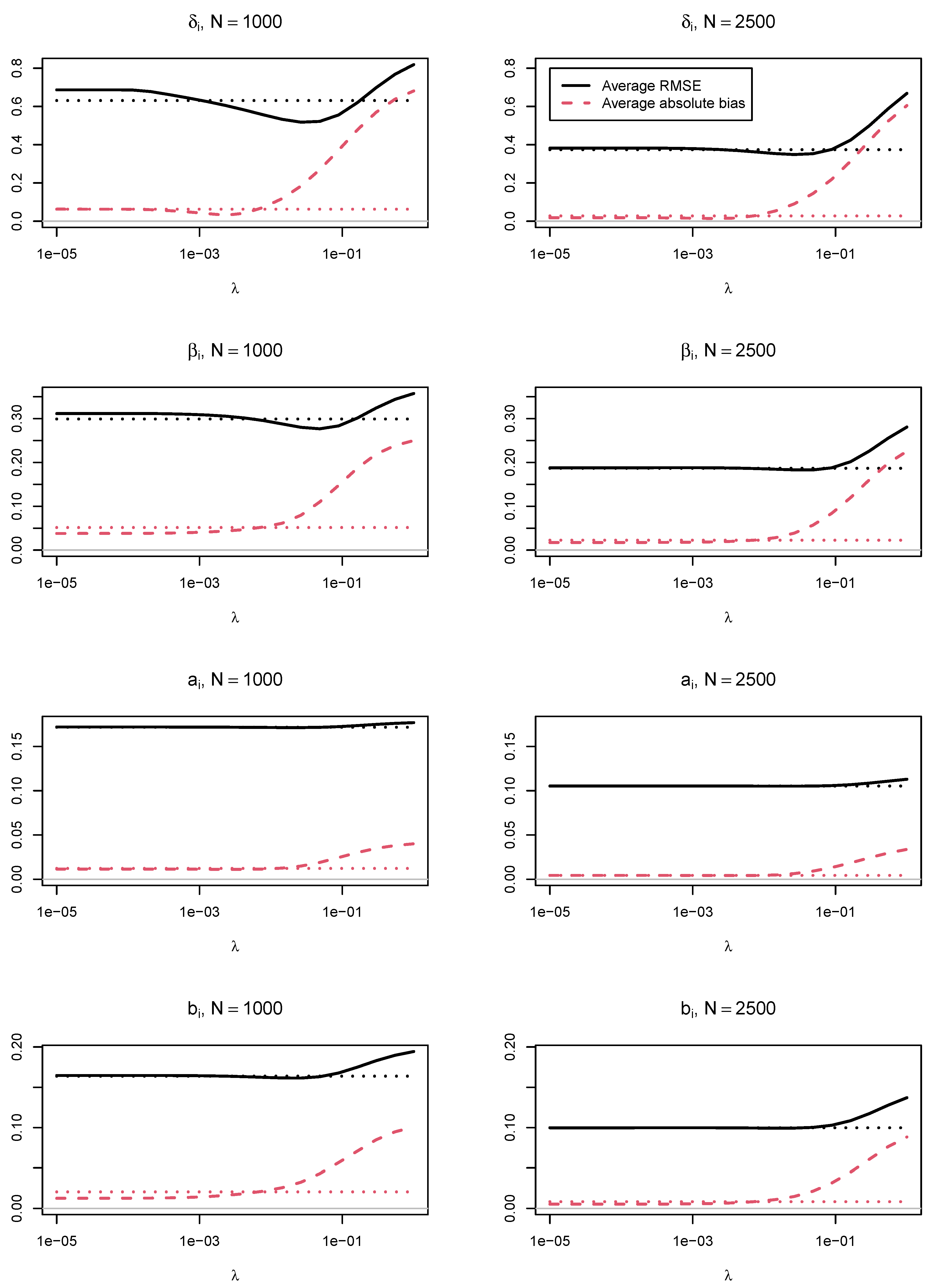
In Figure 2, the average absolute bias (red dashed line) and the average RMSE (solid black line) for item parameter groups δ , β , a, and b are displayed for the DGM2. It can be seen that for N = 1000 , the minimum average RMSE for δ parameters is obtained for a λ value that is substantially larger than the optimal regularization parameter λ opt obtained with k-fold cross-validated log-likelihood estimation. Interestingly, biases in all parameters became relevant for sufficiently large regularization parameters. Hence, the search for an optimal λ parameter regarding RMSE reflects a bias-variance tradeoff. However, it should be emphasized that for a broad range of sufficiently small λ values, the bias and RMSE for item discriminations a i , and item difficulties b i were almost unaffected by the choice of λ .
In Table 1, average absolute bias and average RMSE are displayed for the optimal regularization parameter λ opt , and fixed regularization parameters 10 5 , 0.0263665 , and  10 5 . It can be seen that λ = 0.0263665 strongly outperformed the other λ choices in terms of RMSE for the δ i parameters. However, a nonnegligible bias in δ i and β i parameters was introduced by using this regularization parameter. Nevertheless, inducing too much regularization could stabilize estimated item parameters for the response indicators, while the target parameters a i and b i were almost unaffected by the choice of λ . Hence, one could generally conclude that the MW model should be utilized to estimate the missing response mechanism flexibly. The regularization technique is only applied for stabilizing parameter estimates without introducing relevant bias in target item parameter estimates.

4. Empirical Example

4.1. Method

In the following analysis, item responses of booklet 13 in PIRLS 2011 (i.e., the PIRLS Reader) consisting of 35 items (20 CR items and 15 MC items with four response alternatives) were used. For this booklet, item responses of 968 Austrian (AUT), 809 German (DEU), 901 French (FRA), and 802 Dutch (NLD) students were available. The resulting dataset is used for illustrative purposes in this section. For ease of presentation, all polytomous items were dichotomized, where only the highest scores were recoded as correct. The dataset has been made available as data.pirlsmissing in the R [42] package sirt  [43].
Descriptive analyses showed that the average proportion of missing item responses varied considerably between items and countries (AUT: 0.112, DEU: 0.079, FRA: 0.136, NLD: 0.027). For MC items, the average rate of missing item responses was 0.023 ( S D = 0.016 ). For CR items, the average rate of missing item responses was substantially larger ( M = 0.141 , S D = 0.070 ).
We estimated the nonregularized MW model with freely estimated δ i parameters and compared this model to constrained alternatives. In the LI model [12], all δ i parameters were fixed to zero. In the WR model, all missing item responses are treated as incorrect, which was implemented by fixing all δ i parameters to 9.99 setting the response probabilities effectively to zero for students who do not know the item. Finally, in the MI model, we fixed all δ i parameters to zero and fixed the correlation of θ and ξ to zero. Model comparisons were conducted based on the Akaike information criterion (AIC) and the Bayesian information criterion (BIC).
The MW model was also estimated using regularized estimation. The optimal regularization parameter λ opt was selected by minimizing the negative cross-validated log-likelihood value. The sequence of the regularization parameter λ was selected between 10 8 and 10,000, equidistantly spaced on a logarithmic scale.
The R [42] package sirt [43] using the sirt::xxirt() was employed for fitting the IRT models. Replication material can be found in the directory Empirical Example at https://osf.io/5pd28 (accessed on 21 June 2023).

4.2. Results

In Table 2, model comparisons of the four nonregularized models are displayed. The most general MW model turned out to be the best-fitting model in terms of AIC and BIC. In line with [13], the WR model (i.e., treating missing item responses as incorrect) outperformed the LI model (i.e., treating missing item responses as missing). The standard deviation of ξ slightly varies across models, being smallest when treating missing item responses as wrong in model MW. Also note that the correlation of θ and ξ was practically identical for the models LI, WR, and MW.
In Table 3, estimated item parameters of the regularized Mislevy-Wu model are displayed. Notably, the average δ parameters for CR items ( M = 2.01 , M e d = 1.65 , S D = 1.44 ) were lower than MC items ( M = 0.60 , M e d = 0.03 , S D = 2.06 ). Moreover, the average β i parameter was larger for CR items ( M = 2.70 , M e d = 2.89 , S D = 0.85 ) than for MC items ( M = 6.55 , M e d = 5.75 , S D = 1.84 ), reflecting that the missing proportions for CR items were larger than for MC items.
It is also noteworthy that item discriminations a i hardly varied between the MI and LI model (model MI for CR items: M = 1.41 , M e d = 1.25 , S D = 0.74 ; model LI for CR items: M = 1.41 , M e d = 1.25 , S D = 0.75 ). However, item discriminations a i were larger for models WR ( M = 1.62 , M e d = 1.29 , S D = 1.06 ) and MW ( M = 1.58 , M e d = 1.26 , S D = 1.09 ). Similarly, item difficulties b i did not show practical differences between MI and LI models (model MI for CR items: M = 0.25 , M e d = 0.24 , S D = 0.96 ; model LI for CR items: M = 0.24 , M e d = 0.22 , S D = 0.97 ). In line with expectations, the MW model (CR items: M = 0.14 , M e d = 0.12 , S D = 0.93 ) and the WR model resulted in larger item difficulties (CR items: M = 0.07 , M e d = 0.03 , S D = 0.97 ). The pattern was similar for MC items but less pronounced because the missing proportion rates were smaller for MC items compared to CR items.
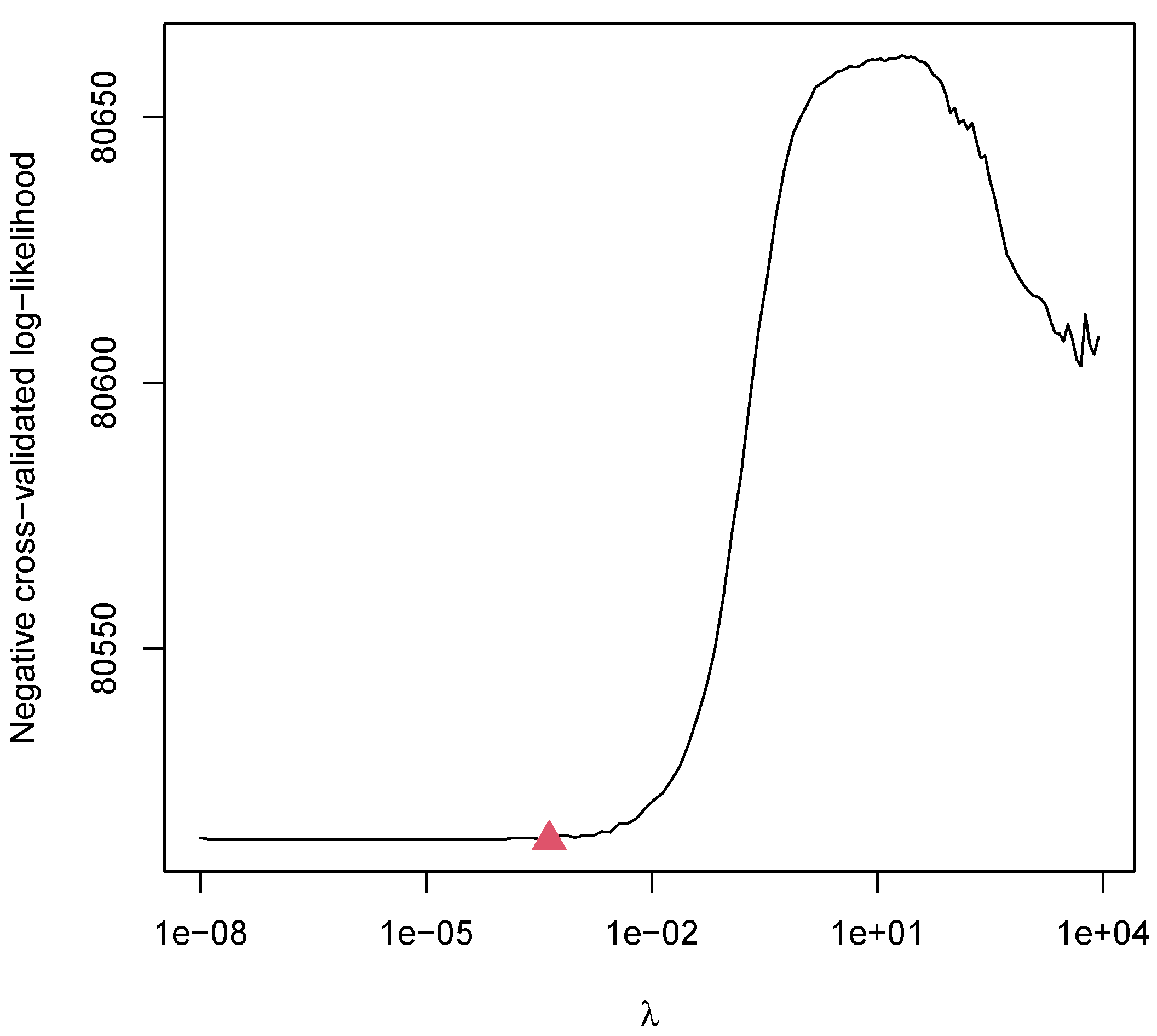
In Figure 3, the negative cross-validated log-likelihood value is displayed as a function of the regularization parameter λ . For sufficiently small λ values, there is almost no difference in cross-validated log-likelihood values. The optimal regularization parameter was estimated as λ opt = 0.0004342 .
In Figure 4, estimated δ i item parameters are displayed as a function of the regularization parameter λ for CR and MC items, respectively. With increasing λ parameters, item parameters are fused to item-format-specific parameters. The fused values were δ i = 3.18 for CR items and δ i = 0.79 for MC items. This result indicated that missing item responses for CR items are more likely associated with a wrong item response than for MC items. Notably, the fused δ i parameters were both negative.
In Figure 5, estimated β i item parameters are displayed as a function of the regularization parameter λ for CR and MC items, respectively. The regularization of the δ i also affected the estimated β i parameters, particularly for MC items.
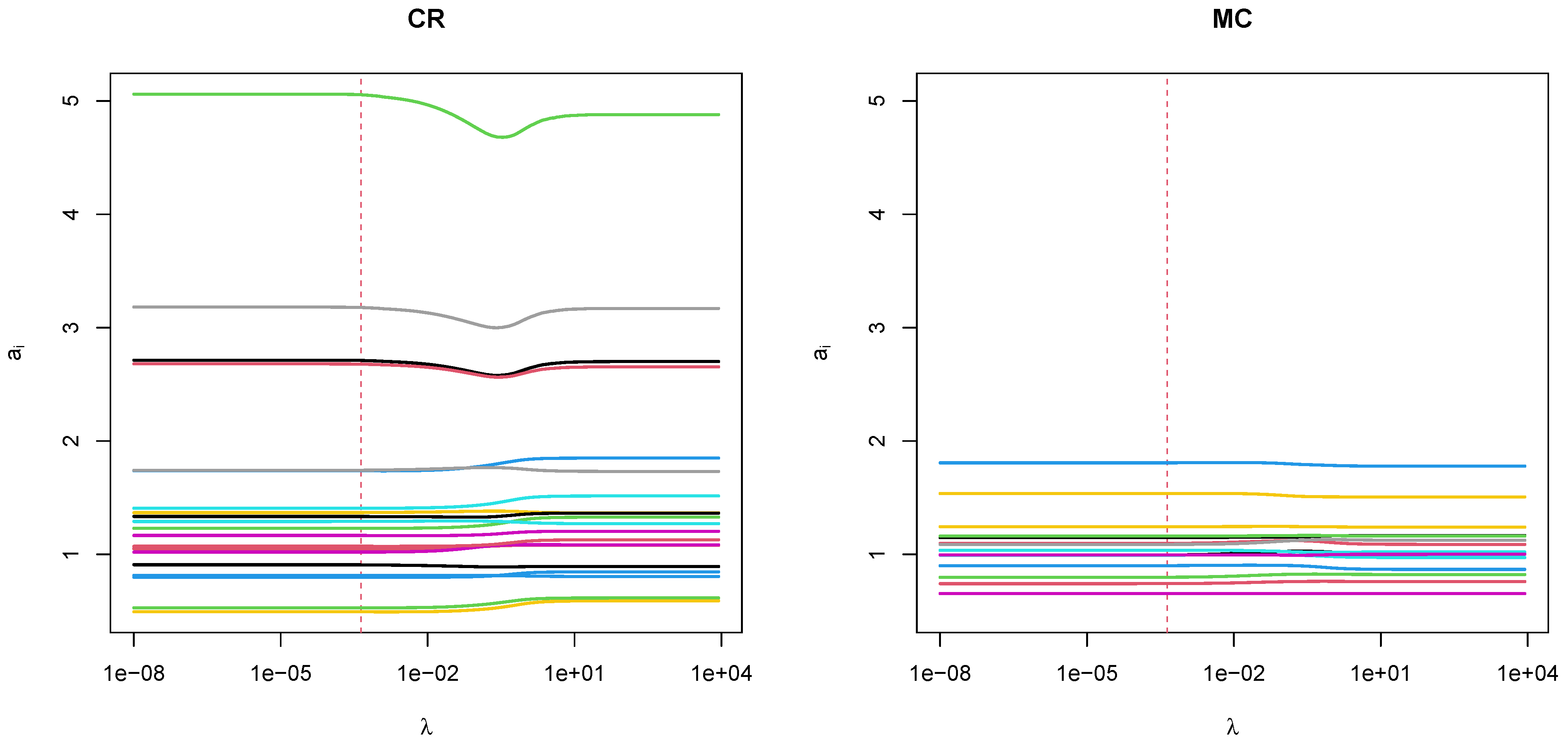
Finally, Figure 6 and Figure 7 display the a i and b i parameters as a function of the regularization parameter λ . The target item parameters are hardly affected for small values of the regularization parameter λ , but show some variation for λ parameters larger than 10 2 .

5. Discussion

In this article, we proposed a regularization estimation approach to the Mislevy-Wu model. This approach allows sufficiently complex missingness mechanisms as well as estimation in moderate sample sizes such as N = 1000 . Interestingly, the most stable item parameter estimates in terms of RMSE were obtained for values of the regularization parameters that were larger than the one obtained by k-fold cross-validation based on the log-likelihood function value.
To further stabilize estimation, the fused ridge penalty function could also involve the β i parameters because they are also difficult to estimate for items with low missing proportion rates or in moderate sample sizes.
It has been shown in the PIRLS 2011 application that the Mislevy-Wu model outperformed all other estimation approaches. Omissions on constructed response items were strongly associated with true item responses. This implies that students who do not know an item likely do not respond to it  [33]. In contrast, multiple-choice items were only weakly associated with true but non-fully observed item responses. Given these findings, it seems plausible in large-scale assessment studies to score omitted constructed response items as wrong while treating multiple-choice as fractionally correct in a pseudo-likelihood estimation approach [44]. In the latter case, a multiple-choice item with K i answer alternative is scored with 1 / K i .
It could be generally argued that constructed response items are omitted more to a lack of knowledge than multiple-choice items. In this sense, as argued by an anonymous reviewer, omissions on constructed response items are likely missing not at random data. In contrast, multiple-choice items could be regarded as missing at random data. In practice, the tendency to omit items can be associated with person traits [45].
The Mislevy-Wu model can be easily extended to item response models for polytomous items. For dichotomous items, the dependence of response indicators R i from true item responses X i is modeled by the item parameter δ i . For polytomous items scored between 0 and K i , K i parameters δ i , k ( k = 1 , , K i ) that differentially weigh the impact of item category k on the response indicator can be identified from the data.
The Mislevy-Wu model can be extended to include covariates for predicting the latent ability θ p and the latent response propensity ξ p [46]. In a latent regression model  [47,48], the estimated item parameters could be fixed, and IRT packages such as TAM  [49] could be utilized for estimation. Such an approach could also be applied in providing plausible values  [50] in LSA studies as realizations of the latent ability θ p that can be used for secondary analysis. In this sense, the Mislevy-Wu model can be implemented in operational practice when scaling item responses in LSA studies such as PISA, PIRLS, or TIMSS [51].
Missing item responses are typically classified into omitted and not-reached item responses [52]. In this article, we only investigated omitted item responses within a test. For speeded tests, it might be preferable not to score not-reached item responses as wrong. However, large-scale assessment studies like PIRLS are not strongly speeded such that there is only a low prevalence of not-reached items.
The Mislevy-Wu model follows a model-based strategy in which the missingness mechanism for the response indicators is simultaneously modeled with the item response model (e.g., 2PL model) of interest. It might be beneficial to weaken the assumption of a unidimensional ability variable θ and unidimensional response propensity variable ξ and to estimate multidimensional variables with an exploratory loading structure  [35] in an imputation model. In this case, the imputation model is more complex than the intentionally misspecified analysis model  [17,53]. Certainly, such an estimation approach would need even larger sample sizes, and regularized estimation could also be applied to the exploratory loading structure.
Although modeling missingness mechanisms in educational studies now receive wide attention, only in rare cases, the dependence of item omissions from the item itself is considered a viable alternative (e.g., see [6]). This is unfortunate because we empirically demonstrated that there are several studies in which treating constructed response items as wrong [13] instead of latent ignorable (i.e., as missing; [6]) resulted in superior model fit. The Mislevy-Wu model contains these two extreme scoring treatments as particular constrained models and also parameterizes processes that are a mixture of both. Hence, if missing item responses should be modeled in large-scale assessment studies, there is no excuse for neglecting the Mislevy-Wu model from the preferred psychometrician’s toolkit.

Funding

This research received no external funding.

Data Availability Statement

The PIRLS 2011 dataset is available at https://timssandpirls.bc.edu/pirls2011/international-database.html (accessed on 21 June 2023). The part of the dataset used in this article can be accessed as the R object data.pirlsmissing in the R package sirt  [43].

Conflicts of Interest

The authors declare no conflict of interest.

Abbreviations

The following abbreviations are used in this manuscript:
2PLtwo-parameter logistic
AICAkaike information criterion
BICBayesian information criterion
CRconstructed response
DGMdata-generating model
IRTitem response theory
LSAlarge-scale assessment
LIlatent ignorability
MARmissing at random
MCmultiple-choice
MImanifest ignorability
MLmaximum likelihood
MNARmissing not at random
MWMislevy-Wu
PIRLSprogress in international reading literacy study
RMSEroot mean square error

Appendix A. Item Parameters Used in the Simulation Study

In Table A1, data-generating item parameters for the simulation study are displayed.
Table A1. Simulation Study: Data-generating item parameters of the Mislevy-Wu model.
ItemType a i b i β i δ i
DGM1DGM2
C01CR 1.7 1.4−1.7 0.3−2.0
C02CR 1.2 0.4−2.7−0.7−1.7
C03CR 0.5 1.3−2.2−0.2−3.6
C04CR 2.2−0.6−1.4 0.6−2.9
C05CR 2.7−0.3−1.3 0.7−3.1
C06CR 2.8−0.1−1.2 0.8−3.8
C07CR 1.3−1.4−2.5−0.5−4.8
C08CR 1.3−1.5−1.8 0.2−2.0
C09CR 1.1−0.4−2.5−0.5−1.3
C10CR 0.5 0.8−2.4−0.4−0.6
M11MC 0.9−1.3−3.2−3.2  0.5
M12MC 1.0−0.4−3.4−3.4−0.8
M13MC 0.7−0.8−3.6−3.6−0.3
M14MC 1.2−0.6−3.7−3.7−0.2
M15MC 1.1−0.8−2.8−2.8  0.4
M16MC 1.2−1.6−2.8−2.8−0.3
M17MC 1.8−1.7−2.8−2.8−1.1
M18MC 1.0−1.1−3.4−3.4−1.0
M19MC 1.0−0.8−2.8−2.8−0.5
M20MC 1.5−2.0−1.8−1.8−0.9
Note. DGM = data-generating model; Type = item format; CR = constructed response item; MC = multiple-choice item.

References

  1. Lietz, P.; Cresswell, J.C.; Rust, K.F.; Adams, R.J. (Eds.) Implementation of Large-Scale Education Assessments; Wiley: New York, NY, USA, 2017. [Google Scholar] [CrossRef]
  2. Rutkowski, L.; von Davier, M.; Rutkowski, D. (Eds.) A Handbook of International Large-Scale Assessment: Background, Technical Issues, and Methods of Data Analysis; Chapman Hall/CRC Press: London, UK, 2013. [Google Scholar] [CrossRef]
  3. Foy, P.; Yin, L. Scaling the PIRLS 2016 achievement data. In Methods and Procedures in PIRLS 2016; Martin, M.O., Mullis, I.V., Hooper, M., Eds.; IEA: Chestnut Hill, MA, USA, 2017. [Google Scholar]
  4. Foy, P.; Yin, L. Scaling the TIMSS 2015 achievement data. In Methods and Procedures in TIMSS 2015; Martin, M.O., Mullis, I.V., Hooper, M., Eds.; IEA: Chestnut Hill, MA, USA, 2016. [Google Scholar]
  5. OECD. PISA 2018. Technical Report; OECD: Paris, France, 2020; Available online: https://bit.ly/3zWbidA (accessed on 21 June 2023).
  6. Pohl, S.; Ulitzsch, E.; von Davier, M. Reframing rankings in educational assessments. Science 2021, 372, 338–340. [Google Scholar] [CrossRef] [PubMed]
  7. Mislevy, R.J. Missing responses in item response modeling. In Handbook of Item Response Theory, Vol. 2: Statistical Tools; van der Linden, W.J., Ed.; CRC Press: Boca Raton, FL, USA, 2016; pp. 171–194. [Google Scholar] [CrossRef]
  8. Bock, R.D.; Moustaki, I. Item response theory in a general framework. In Handbook of Statistics, Vol. 26: Psychometrics; Rao, C.R., Sinharay, S., Eds.; Elsevier: Amsterdam, The Netherlands, 2007; pp. 469–513. [Google Scholar] [CrossRef]
  9. van der Linden, W.J.; Hambleton, R.K. (Eds.). Handbook of Modern Item Response Theory; Springer: New York, NY, USA, 1997. [Google Scholar] [CrossRef]
  10. van der Linden, W.J. Unidimensional logistic response models. In Handbook of Item Response Theory, Volume 1: Models; van der Linden, W.J., Ed.; CRC Press: Boca Raton, FL, USA, 2016; pp. 11–30. [Google Scholar]
  11. Rose, N.; von Davier, M.; Nagengast, B. Modeling omitted and not-reached items in IRT models. Psychometrika 2017, 82, 795–819. [Google Scholar] [CrossRef] [PubMed]
  12. Holman, R.; Glas, C.A.W. Modelling non-ignorable missing-data mechanisms with item response theory models. Brit. J. Math. Stat. Psychol. 2005, 58, 1–17. [Google Scholar] [CrossRef]
  13. Robitzsch, A. On the treatment of missing item responses in educational large-scale assessment data: An illustrative simulation study and a case study using PISA 2018 mathematics data. Eur. J. Investig. Health Psychol. Educ. 2021, 11, 1653–1687. [Google Scholar] [CrossRef]
  14. Guo, J.; Xu, X. An IRT-based model for omitted and not-reached items. arXiv 2019, arXiv:1904.03767. [Google Scholar] [CrossRef]
  15. Mislevy, R.J.; Wu, P.K. Missing Responses and IRT Ability Estimation: Omits, Choice, Time Limits, and Adaptive Testing; (Research Report No. RR-96-30); Educational Testing Service: Princeton, NJ, USA, 1996. [Google Scholar] [CrossRef]
  16. Rosas, G.; Shomer, Y.; Haptonstahl, S.R. No news is news: Nonignorable nonresponse in roll-call data analysis. Am. J. Political Sci. 2015, 59, 511–528. [Google Scholar] [CrossRef]
  17. Robitzsch, A.; Lüdtke, O. Some thoughts on analytical choices in the scaling model for test scores in international large-scale assessment studies. Meas. Instrum. Soc. Sci. 2022, 4, 9. [Google Scholar] [CrossRef]
  18. Little, R.J.A.; Rubin, D.B. Statistical Analysis with Missing Data; Wiley: New York, NY, USA, 2002. [Google Scholar] [CrossRef] [Green Version]
  19. Rubin, D.B. Inference and missing data. Biometrika 1976, 63, 581–592. [Google Scholar] [CrossRef]
  20. Seaman, S.; Galati, J.; Jackson, D.; Carlin, J. What is meant by "missing at random"? Stat. Sci. 2013, 28, 257–268. [Google Scholar] [CrossRef] [Green Version]
  21. Frangakis, C.E.; Rubin, D.B. Addressing complications of intention-to-treat analysis in the combined presence of all-or-none treatment-noncompliance and subsequent missing outcomes. Biometrika 1999, 86, 365–379. [Google Scholar] [CrossRef]
  22. Harel, O.; Schafer, J.L. Partial and latent ignorability in missing-data problems. Biometrika 2009, 96, 37–50. [Google Scholar] [CrossRef]
  23. Beesley, L.J.; Taylor, J.M.G.; Little, R.J.A. Sequential imputation for models with latent variables assuming latent ignorability. Aust. N. Z. J. Stat. 2019, 61, 213–233. [Google Scholar] [CrossRef]
  24. Debeer, D.; Janssen, R.; De Boeck, P. Modeling skipped and not-reached items using IRTrees. J. Educ. Meas. 2017, 54, 333–363. [Google Scholar] [CrossRef]
  25. Glas, C.A.W.; Pimentel, J.L.; Lamers, S.M.A. Nonignorable data in IRT models: Polytomous responses and response propensity models with covariates. Psychol. Test Assess. Model. 2015, 57, 523–541. [Google Scholar]
  26. Bartolucci, F.; Montanari, G.E.; Pandolfi, S. Latent ignorability and item selection for nursing home case-mix evaluation. J. Classif. 2018, 35, 172–193. [Google Scholar] [CrossRef]
  27. Kuha, J.; Katsikatsou, M.; Moustaki, I. Latent variable modelling with non-ignorable item nonresponse: Multigroup response propensity models for cross-national analysis. J. R. Stat. Soc. Ser. A Stat. Soc. 2018, 181, 1169–1192. [Google Scholar] [CrossRef] [Green Version]
  28. Albert, P.S.; Follmann, D.A. Shared-parameter models. In Longitudinal Data Analysis; Fitzmaurice, G., Davidian, M., Verbeke, G., Molenberghs, G., Eds.; Chapman and Hall/CRC: Boca Raton, FL, USA, 2008; pp. 447–466. [Google Scholar] [CrossRef] [Green Version]
  29. Little, R.J. Selection and pattern-mixture models. In Longitudinal Data Analysis; Fitzmaurice, G., Davidian, M., Verbeke, G., Molenberghs, G., Eds.; Chapman and Hall/CRC: Boca Raton, FL, USA, 2008; pp. 409–431. [Google Scholar] [CrossRef] [Green Version]
  30. Birnbaum, A. Some latent trait models and their use in inferring an examinee’s ability. In Statistical Theories of Mental Test Scores; Lord, F.M., Novick, M.R., Eds.; MIT Press: Reading, MA, USA, 1968; pp. 397–479. [Google Scholar]
  31. Deribo, T.; Kroehne, U.; Goldhammer, F. Model-based treatment of rapid guessing. J. Educ. Meas. 2021, 58, 281–303. [Google Scholar] [CrossRef]
  32. Robitzsch, A.; Lüdtke, O. An item response model for omitted responses in performance tests. Personal communication. 2017. [Google Scholar]
  33. Robitzsch, A. Nonignorable consequences of (partially) ignoring missing item responses: Students omit (constructed response) items due to a lack of knowledge. Knowledge 2023, 3, 215–231. [Google Scholar] [CrossRef]
  34. Kreitchmann, R.S.; Abad, F.J.; Ponsoda, V. A two-dimensional multiple-choice model accounting for omissions. Front. Psychol. 2018, 9, 2540. [Google Scholar] [CrossRef]
  35. Rose, N.; von Davier, M.; Nagengast, B. Commonalities and differences in IRT-based methods for nonignorable item nonresponses. Psych. Test Assess. Model. 2015, 57, 472–498. [Google Scholar]
  36. Köhler, C.; Pohl, S.; Carstensen, C.H. Taking the missing propensity into account when estimating competence scores: Evaluation of item response theory models for nonignorable omissions. Educ. Psychol. Meas. 2015, 75, 850–874. [Google Scholar] [CrossRef] [PubMed] [Green Version]
  37. Xu, X.; von Davier, M. Fitting the Structured General Diagnostic Model to NAEP Data; (Research Report No. RR-08-28); Educational Testing Service: Princeton, NJ, USA, 2008. [Google Scholar] [CrossRef]
  38. Aitkin, M. Expectation maximization algorithm and extensions. In Handbook of Item Response Theory, Vol. 2: Statistical Tools; van der Linden, W.J., Ed.; CRC Press: Boca Raton, FL, USA, 2016; pp. 217–236. [Google Scholar] [CrossRef]
  39. Hanson, B. IRT Parameter Estimation Using the EM Algorithm. 2000. Technical Report. Available online: https://bit.ly/3i4pOdg (accessed on 21 June 2023).
  40. Battauz, M. Regularized estimation of the four-parameter logistic model. Psych 2020, 2, 269–278. [Google Scholar] [CrossRef]
  41. Bates, S.; Hastie, T.; Tibshirani, R. Cross-validation: What does it estimate and how well does it do it? J. Am. Stat. Assoc. 2023. [Google Scholar] [CrossRef]
  42. R Core Team. R: A Language and Environment for Statistical Computing; R Core Team: Vienna, Austria, 2023; Available online: https://www.R-project.org/ (accessed on 15 March 2023).
  43. Robitzsch, A. sirt: Supplementary Item Response Theory Models. R Package Version 3.13-151. 2023. Available online: https://github.com/alexanderrobitzsch/sirt (accessed on 23 April 2023).
  44. Lord, F.M. Estimation of latent ability and item parameters when there are omitted responses. Psychometrika 1974, 39, 247–264. [Google Scholar] [CrossRef]
  45. Hitt, C.; Trivitt, J.; Cheng, A. When you say nothing at all: The predictive power of student effort on surveys. Econ. Educ. Rev. 2016, 52, 105–119. [Google Scholar] [CrossRef]
  46. Köhler, C.; Pohl, S.; Carstensen, C.H. Investigating mechanisms for missing responses in competence tests. Psych. Test Assess. Model. 2015, 57, 499–522. [Google Scholar]
  47. Mislevy, R.J. Randomization-based inference about latent variables from complex samples. Psychometrika 1991, 56, 177–196. [Google Scholar] [CrossRef]
  48. von Davier, M.; Sinharay, S. Analytics in international large-scale assessments: Item response theory and population models. In A handbook of International Large-Scale Assessment: Background, Technical Issues, and Methods of Data Analysis; Rutkowski, L., von Davier, M., Rutkowski, D., Eds.; Chapman Hall/CRC Press: London, UK, 2013; pp. 155–174. [Google Scholar] [CrossRef]
  49. Robitzsch, A.; Kiefer, T.; Wu, M. TAM: Test Analysis Modules. R Package Version 4.1-4. 2022. Available online: https://CRAN.R-project.org/package=TAM (accessed on 28 August 2022).
  50. Wu, M. The role of plausible values in large-scale surveys. Stud. Educ. Eval. 2005, 31, 114–128. [Google Scholar] [CrossRef]
  51. von Davier, M. Omitted response treatment using a modified Laplace smoothing for approximate Bayesian inference in item response theory. PsyArXiv 2023. [Google Scholar] [CrossRef]
  52. Gorgun, G.; Bulut, O. A polytomous scoring approach to handle not-reached items in low-stakes assessments. Educ. Psychol. Meas. 2021, 81, 847–871. [Google Scholar] [CrossRef]
  53. Robitzsch, A. On the choice of the item response model for scaling PISA data: Model selection based on information criteria and quantifying model uncertainty. Entropy 2022, 24, 760. [Google Scholar] [CrossRef]
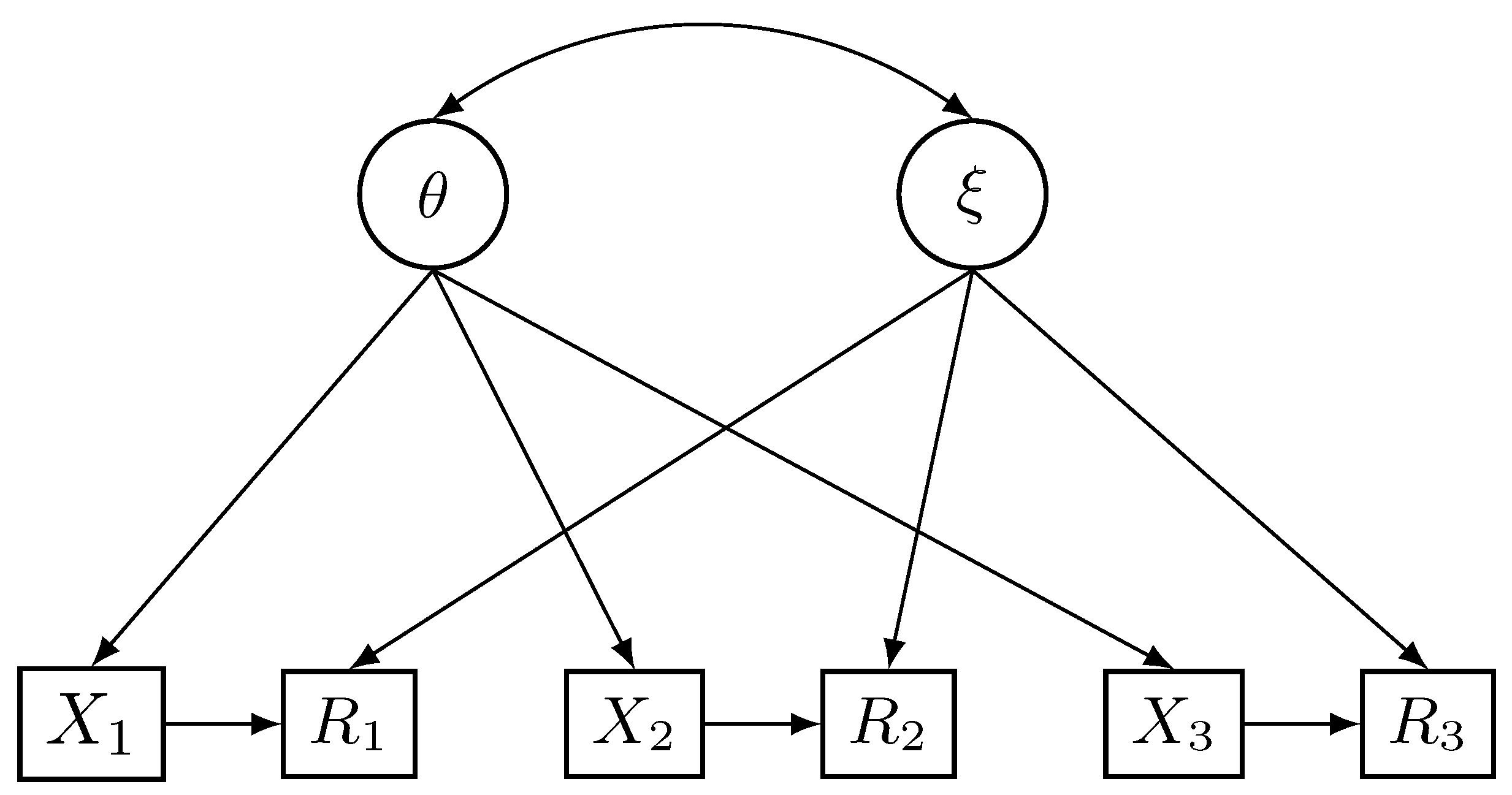
Figure 1. Graphical representation of the Mislevy-Wu model with three items X 1 , X 2 , and X 3 , and their corresponding response indicators R 1 , R 2 , and R 3 , and latent ability θ and latent response propensity ξ .
Information 14 00368 g001
Figure 2. Average absolute bias and average root mean square error (RMSE) for item parameter groups of the regularized Mislevy-Wu model for data-generating model DGM2 as a function of sample size N and the regularization parameter λ . RMSE and bias values for the optimal regularization parameter λ opt selected with cross-validated log-likelihood are displayed with dotted lines.
Information 14 00368 g002
Figure 3. Negative cross-validated log-likelihood value as a function of the regularization parameter λ . The optimal regularization parameter λ opt selected with cross-validated log-likelihood is displayed with a red triangle.
Information 14 00368 g003
Figure 4. Curves of item parameter estimates δ i are shown as a function of the regularization parameter λ for constructed response (CR) items (left panel) and multiple-choice (MC) items (right panel). The optimal regularization parameter λ opt selected with cross-validated log-likelihood is displayed with a red dashed line.
Information 14 00368 g004
Figure 5. Curves of item parameter estimates β i as a function of the regularization parameter λ for constructed response (CR) items (left panel) and multiple-choice (MC) items (right panel). The optimal regularization parameter λ opt selected with cross-validated log-likelihood is displayed with a red dashed line.
Information 14 00368 g005
Figure 6. Curves of item parameter estimates a i as a function of the regularization parameter λ for constructed response (CR) items (left panel) and multiple-choice (MC) items (right panel). The optimal regularization parameter λ opt selected with cross-validated log-likelihood is displayed with a red dashed line.
Information 14 00368 g006
Figure 7. Curves of item parameter estimates b i as a function of the regularization parameter λ for constructed response (CR) items (left panel) and multiple-choice (MC) items (right panel). The optimal regularization parameter λ opt selected with cross-validated log-likelihood is displayed with a red dashed line.
Information 14 00368 g007
Table 1. Simulation Study: Average absolute bias (Bias) and average absolute RMSE of estimated item parameters of the regularized Mislevy-Wu model as a function of sample size N and different choices of the regularization parameter λ for two data-generating models (DGM) DGM1 and DGM2.
DGMParNBias for λ = RMSE for λ =
10 5 λ opt 0.0263665 10 5 10 5 λ opt 0.0263665 10 5
DGM1 δ i 10000.1230.0760.3040.7540.9150.8450.6380.875
25000.0670.0450.1900.7570.5630.5400.4510.812
β i 10000.0630.0680.0920.2210.3130.3090.2850.329
25000.0280.0310.0520.2210.1890.1890.1860.277
a i 10000.0080.0080.0110.0280.1540.1540.1540.156
25000.0020.0020.0050.0280.0960.0960.0960.102
b i 10000.0160.0180.0280.0640.1460.1460.1440.154
25000.0080.0100.0170.0620.0890.0900.0900.109
DGM2 δ i 10000.0630.0630.1840.7500.6870.6310.5180.896
25000.0180.0280.0900.7500.3820.3740.3490.822
β i 10000.0380.0520.0800.2660.3110.2990.2800.376
25000.0170.0230.0390.2670.1880.1870.1830.323
a i 10000.0120.0120.0150.0430.1720.1720.1710.178
25000.0040.0040.0060.0410.1050.1050.1050.118
b i 10000.0130.0200.0320.1080.1650.1640.1610.201
25000.0050.0080.0150.1050.1000.1000.0990.155
Note. Par = item parameter group; λ opt  = optimal regularization parameter selected with cross-validated log-likelihood.
Table 2. PIRLS Reader 2011: Model comparisons.
Model#nparsAICBIC SD ( ξ ) Cor ( θ , ξ ) δ i
MI106162,192162,8442.41 00 99
LI107161,796162,4542.380.41  99
WR107161,414162,0732.290.41  −9.99 
MW142161,086161,9602.340.41  est
Note. #npars = number of estimated model parameters; MI = manifest ignorabiity; LI = latent ignorability; WR = treating missing item responses as wrong (i.e., 0); MW = Mislevy-Wu model; ‡ = fixed model parameter; est =  estimated model parameters; Entries with the least AIC or BIC are printed in bold font, respectively.
Table 3. PIRLS Reader 2011: Estimated item parameters of the regularized Mislevy-Wu model.
a i b i β i δ i
ItemTypeFreq0Freq1FreqNAMILIWRMWMILIWRMWMWMW
R31G02CCR 0.28 0.64 0.08 0.86 0.85 0.89 0.91−1.04−1.04−0.81−0.80−3.03−4.45
R31G04CCR 0.58 0.21 0.20 1.05 1.04 1.06 1.05 1.23 1.25 1.43 1.36−2.34−1.40
R31G08CZCR 0.41 0.40 0.19 1.27 1.26 1.34 1.23 0.18 0.20 0.48 0.30−2.01−0.90
R31G08CACR 0.40 0.37 0.23 1.76 1.74 1.82 1.74 1.32 1.35 1.44 1.39−1.99−0.76
R31G08CBCR 0.61 0.14 0.25 1.45 1.44 1.51 1.41 0.09 0.11 0.31 0.17−2.41−0.79
R31G10CCR 0.48 0.40 0.13 1.13 1.13 1.20 1.17 0.28 0.29 0.40 0.35−3.08−1.42
R31G12CCR 0.51 0.29 0.20 0.49 0.48 0.63 0.49 1.24 1.26 1.47 1.25−2.53−0.04
R31G13CZCR 0.17 0.66 0.17 2.43 2.46 3.31 3.18−0.55−0.53−0.27−0.33−1.55−2.81
R31G13CACR 0.23 0.58 0.20 2.11 2.12 2.85 2.72−0.36−0.34−0.11−0.14−1.35−3.40
R31G13CBCR 0.26 0.52 0.22 2.19 2.19 2.75 2.68−0.12−0.10 0.07 0.05−1.54−3.21
R31G13CCCR 0.32 0.46 0.22 3.58 3.67 4.88 5.07−0.76−0.74−0.51−0.57−1.69−2.69
R31P02CCR 0.23 0.73 0.04 0.81 0.81 0.79 0.81−1.61−1.62−1.52−1.48−3.77−3.88
R31P03CCR 0.16 0.79 0.06 1.26 1.25 1.24 1.29−1.57−1.57−1.42−1.38−2.88−4.36
R31P05CCR 0.45 0.48 0.08 1.08 1.09 1.07 1.02−0.05−0.05 0.04−0.11−4.51 0.59
R31P06CCR 0.19 0.76 0.04 1.40 1.39 1.34 1.37−1.28−1.28−1.23−1.24−3.85−2.43
R31P07CCR 0.19 0.74 0.07 1.74 1.74 1.67 1.74−1.08−1.08−0.98−0.98−2.90−3.12
R31P09CCR 0.14 0.80 0.06 1.25 1.26 1.37 1.33−1.71−1.68−1.40−1.55−3.40−1.83
R31P14CCR 0.33 0.54 0.13 1.06 1.06 1.15 1.07−0.48−0.47−0.24−0.39−2.92−1.22
R31P15CCR 0.51 0.36 0.13 0.52 0.53 0.63 0.53 0.74 0.75 0.92 0.81−3.19−0.55
R31P16CCR 0.49 0.38 0.13 0.76 0.75 0.86 0.80 0.48 0.49 0.62 0.57−3.03−1.48
R31G01MMC 0.18 0.81 0.01 1.11 1.15 1.13 1.15−1.66−1.63−1.66−1.68−10.51 4.20
R31G03MMC 0.26 0.73 0.01 1.19 1.18 1.04 1.10−1.11−1.11−1.24−1.23−7.52 1.24
R31G05MMC 0.42 0.56 0.02 0.84 0.85 0.81 0.80−0.41−0.40−0.42−0.50−7.56 2.18
R31G06MMC 0.27 0.72 0.01 0.98 0.97 0.84 0.90−1.20−1.22−1.38−1.30−5.72−2.94
R31G07MMC 0.40 0.58 0.02 1.04 1.04 0.95 0.99−0.41−0.41−0.45−0.45−5.64−0.82
R31G09MMC 0.38 0.60 0.02 0.69 0.69 0.65 0.65−0.71−0.71−0.74−0.78−6.06 0.08
R31G11MMC 0.36 0.62 0.02 1.25 1.26 1.23 1.24−0.54−0.54−0.56−0.58−5.81 0.03
R31G14MMC 0.33 0.60 0.07 1.16 1.17 1.07 1.09−0.65−0.64−0.53−0.79−5.41 1.68
R31P01MMC 0.25 0.74 0.01 1.06 1.06 0.97 0.99−1.24−1.24−1.33−1.37−9.84 3.88
R31P04MMC 0.53 0.46 0.01 0.76 0.77 0.75 0.74 0.19 0.19 0.17 0.12−8.56 3.12
R31P08MMC 0.19 0.79 0.02 1.19 1.21 1.13 1.16−1.52−1.51−1.53−1.58−5.75−0.01
R31P10MMC 0.11 0.87 0.03 1.88 1.89 1.74 1.81−1.66−1.65−1.65−1.69−4.80−1.29
R31P11MMC 0.27 0.70 0.03 1.07 1.07 1.04 1.04−1.05−1.05−1.05−1.09−5.18−0.78
R31P12MMC 0.33 0.64 0.03 1.02 1.03 1.02 1.00−0.77−0.76−0.75−0.80−5.33−0.32
R31P13MMC 0.09 0.88 0.03 1.59 1.60 1.49 1.54−1.97−1.96−1.90−1.99−4.53−1.28
Note. Type  = item format; CR = constructed response item; MC = multiple-choice item; MI = manifest ignorabiity; LI = latent ignorability; WR = treating missing item responses as wrong (i.e., 0); MW = Mislevy-Wu model.
Disclaimer/Publisher’s Note: The statements, opinions and data contained in all publications are solely those of the individual author(s) and contributor(s) and not of MDPI and/or the editor(s). MDPI and/or the editor(s) disclaim responsibility for any injury to people or property resulting from any ideas, methods, instructions or products referred to in the content.