AutoML with Bayesian Optimizations for Big Data Management

Abstract

The field of automated machine learning (AutoML) has gained significant attention in recent years due to its ability to automate the process of building and optimizing machine learning models. However, the increasing amount of big data being generated has presented new challenges for AutoML systems in terms of big data management. In this paper, we introduce Fabolas and learning curve extrapolation as two methods for accelerating hyperparameter optimization. Four methods for quickening training were presented including Bag of Little Bootstraps, k-means clustering for Support Vector Machines, subsample size selection for gradient descent, and subsampling for logistic regression. Additionally, we also discuss the use of Markov Chain Monte Carlo (MCMC) methods and other stochastic optimization techniques to improve the efficiency of AutoML systems in managing big data. These methods enhance various facets of the training process, making it feasible to combine them in diverse ways to gain further speedups. We review several combinations that have potential and provide a comprehensive understanding of the current state of AutoML and its potential for managing big data in various industries. Furthermore, we also mention the importance of parallel computing and distributed systems to improve the scalability of the AutoML systems while working with big data.

1. Introduction

Automated Machine Learning (AutoML) can be applied to Big Data processing, management, and systems in several ways. One way is by using AutoML to automatically optimize the performance of machine learning models on large datasets. This can include selecting the most appropriate algorithm, tuning hyperparameters, and selecting features. Another way is to use AutoML to automate the process of building and deploying machine learning models in a big data environment. For example, AutoML can be used to automatically scale and distribute models across a cluster of machines or to automatically select the best storage and processing options for a given dataset. Additionally, AutoML can also be used for automating feature engineering on big data. This can help to reduce the time and effort required to prepare large datasets for machine learning. Automated Machine Learning (AutoML) refers to the process of automating the entire machine learning pipeline, from data preprocessing to model selection, training, and deployment. There are several techniques used in AutoML to achieve this automation. Some of the most common techniques include:

• Hyperparameter tuning: This involves automatically searching for the best combination of hyperparameters for a given machine-learning model. This can be done using techniques such as grid search, random search, or Bayesian optimization.
• Feature selection and engineering: AutoML can be used to automatically select the most relevant features for a given dataset and to perform feature engineering tasks such as scaling, normalization, and dimensionality reduction.
• Model selection: AutoML can be used to automatically select the best machine learning model for a given dataset. This can be done by comparing the performance of different models on the dataset, or by using techniques such as ensembling or stacking to combine the predictions of multiple models.
• Neural Architecture Search (NAS): This is a subfield of AutoML that aims to automate the design of neural network architectures. The goal is to find the best neural network architecture for a given task and dataset [1,2,3,4].
• Automated Deployment: AutoML can be used to automate the process of deploying machine learning models into production. This can include tasks such as model versioning, monitoring, and scaling.

Overall, the goal of AutoML is to make the process of building and deploying machine learning models faster, easier, and more accessible to non-experts by automating many of the time-consuming and tedious tasks involved in the machine learning pipeline.

Big Data processing has grown in significance over the previous few years across a wide range of industries. For machine learning applications, this growth in data volume presents new challenges. In most cases, the size of the training dataset has a polynomial effect on how long learners require to train ${\mathcal{D}}_{\mathit{train}}$, i.e., $\mathcal{O}\left(\right|{\mathcal{D}}_{\mathit{train}}{|}^{\alpha }),\alpha \ge 1$. Always utilizing the complete dataset rapidly becomes impractical since cross-validation and hyperparameter search iterations require that training be repeated. This paper provides an overview of methods for addressing this issue with an emphasis on classification challenges.

Finding a hypothesis may often be divided into three stages:

• Model selection: It is necessary to first use a model to identify the class of hypothesis spaces from which the final hypothesis will be selected. The model of choice is typically embedded implicitly in the class of hypothesis spaces of a learner L. Automating this procedure is challenging. The model is chosen, in practice, by experts who have a thorough grasp of the problem at hand.
• Hyperparameter search: Optimizing a vector $\lambda$ in the hyperparameter space ${\Lambda }_L$ of the learner L representing a hypothesis space ${\mathcal{H}}_{\lambda }$. A naïve approach to do this is to systematically try configurations using a grid search or a random search over ${\Lambda }_L$. To evaluate the quality of a given $\lambda$, L is usually trained on a training dataset ${\mathcal{D}}_{\mathit{train}}$ using $\lambda$. This yields a hypothesis ${\widehat{h}}_{\lambda }\in {\mathcal{H}}_{\lambda }$ that is evaluated using a validation dataset ${\mathcal{D}}_{\mathit{valid}}$. The goal of hyperparameter optimization is to minimize the loss $l\left(\lambda \right)$ of ${\widehat{h}}_{\lambda }$ on ${\mathcal{D}}_{\mathit{valid}}$, i.e., to find an approximation:

  $$[\widehat{\lambda }={\lambda }^{\ast }:={argmin}_{\lambda }l\left(\lambda \right)]$$

  (1)
• Training or parameter search: Let w be a vector in the parameter space $W_{{\mathcal{H}}_{\lambda }}$, describing a hypothesis $h_{\lambda ,w}\in {\mathcal{H}}_{\lambda }$ given a hyperparameter configuration $\lambda$. The goal of parameter search is to find an approximation ${\widehat{h}}_{\lambda }$ of the hypothesis $h_{\lambda }^{\ast }:=arg{min}_{h_{\lambda ,w}}\ell \left({\mathcal{D}}_{\mathit{train}}\right|h_{\lambda ,w})$, with $\ell \left({\mathcal{D}}_{\mathit{train}}\right|h_{\lambda ,w})$ being the empirical loss of $h_{\lambda ,w}$ on a given training dataset ${\mathcal{D}}_{\mathit{train}}$ according to some loss function ℓ. Depending on the learner L, various kinds of optimization methods are used to find this minimum, e.g., Bayesian optimization, quadratic programming or, if ${\nabla }_{w}e\left({\mathcal{D}}_{\mathit{train}}\right|h_{\lambda ,w})$ is computable, gradient descent. The quality l of ${\widehat{h}}_{\lambda }$ is measured by the loss on a validation or test dataset, i.e.,

  $$[l\left(\lambda \right)=\ell ({\mathcal{D}}_{\mathit{valid}}\mid {\widehat{h}}_{\lambda })]$$

  (2)

This article is organized in accordance that the learner L is provided. The methods for accelerating the hyperparameter search are described in Section 3. Furthermore, in Section 4, it is explained how to enhance the way current learners are trained. In Section 5 the discussion and contribution of this work compared to the state-of-the-art methods take place and finally, in Section 6 the Conclusions and Future Directions are presented. Ultimately, the majority of the methods presented in this paper enhance separate steps in the hypothesis-seeking process, enabling their effective combination.

2. Related Work

In this section, we have provided an overview of related work in various aspects of AutoML, such as feature engineering, meta-learning, neural architecture search, and combined model selection and hyperparameter optimization. We have also discussed the CASH problem, Bayesian optimization, and model-free techniques for hyperparameter optimization. Furthermore, we have presented recent studies and surveys in TinyML, AutoML for anomaly detection, and medical applications, as well as various hyperparameter optimization methods and studies.

2.1. Automated Machine Learning in Industry

Machine learning has become more widely applied in several industries in recent years. Businesses may be more proactive and boost productivity by using industrial applications like defect detection [5] and predictive maintenance [6,7]. Patient data have aided in the treatment of complex diseases like multiple sclerosis and helped doctors choose the most suitable drug in the healthcare industry, to reference [8]. In the insurance and banking sectors, it is feasible to forecast the risks involved with loan applications [9] and claims processing [10,11], allowing for the automatic identification of fraudulent behaviours. Last but not least, improvements in sales and revenue forecasts support supply chain optimization, according to [12].

It takes time and is prone to errors to manually build these actionable machine learning models that may have economic value. Instead, the performance of several models should be assessed while considering diverse methods, hyperparameter tuning, and feature selection into consideration. An ideal option for automation is this incredibly iterative process. The data scientist may now focus on more creative tasks thanks to AutoML, which frees them up from this tedious task and increases the value of the business. By using fast prototyping, new business cases may be found, assessed, and validated.

In the real world, AutoML could provide many insights. Early feedback on the data’s appropriateness for anticipating the given target may come by running a variety of models on the input data. There may be an indication of insufficient predictive power in the data if there are several models built using a wide range of methodologies and they perform similarly to the baseline. In theory, however, reliable models will be produced, giving the data scientist the choice of using the best model that was generated or building an ensemble of several models [13]. The optimization of the feature set via AutoML has a by-product, too: A feature relevance estimate based on the characteristics used as model inputs may be produced via statistical analysis of model quality.

2.2. Feature Engineering and Selection

Researchers have been driven to automate various steps in the machine learning pipeline as a result of the problem of manual hyperparameter tuning [14], including feature engineering [15], meta-learning [16], architecture search [17], and full Combined Model Selection and Hyperparameter optimization [18]. We examine these topics below.

Feature engineering: The research discusses the challenges associated with representation learning, feature preprocessing, and selecting the best discriminating features for a given classification or regression task. Gaudel and Sebag [19] approach feature engineering as a single-player game and train a reinforcement learning-based agent to select the most beneficial traits. To do this, they first model the feature selection problem as a Markov Decision Process (MDP). They also imply a connection between a reward and the eventual status generalization error. The agent develops a tactic that reduces the overall generalization error. Overall, Gaudel’s and Sebag’s approaches to feature engineering using reinforcement learning show promise in improving the performance of classification and regression models by selecting the most informative features.

To find the most discriminating features, Explorekit [20] not only selects the features repeatedly but also creates new candidate features. Katz et al. create unary features by using a single feature with normalization and discrimination operations. They not only combine two or more features to create new candidates, but they also use meta-features collected from the datasets and candidates to train a feature rank estimator. The feature with the highest rank that improves classification accuracy beyond a certain threshold is added to the selected feature set in each cycle.

The Learning Feature Engineering (LFE) approach is a technique aimed at reducing the computational cost associated with iterative feature selection procedures by learning from previous trials the effectiveness of different modifications. The primary objective of the LFE approach is to derive a discriminant feature representation that can improve the performance of classification or regression models. Learning Feature Engineering (LFE) [21] learns from previous trials the efficacy of a modification in order to minimize the computing cost of iterative feature selection procedures. A discriminant feature representation is calculated after mapping the original feature space with the best transformation.

An automated feature selection method based on regression is called AutoLearn [22]. Filtering the initial features and eliminating those that offer little information gain is the first step of the recommended method. Then feature pairs are filtered based on distance correlation to remove dependent pairings. The new features are developed based on the remaining pairs using ridge regression. The best characteristics are those that provide the most stability and knowledge gain, according to [23]. Gene expression data is one of the datasets with which AutoLearn has been used.

2.3. Meta-Learning

By employing metadata about the problem at hand, such as the dataset and the available algorithms and their settings, meta-learning techniques try to improve the performance of an AutoML system. The field is often applied to itself by employing machine learning techniques to acquire and analyze this metainformation. The performance statistics of straightforward algorithms frequently make up the metadata cited in [24], which is the metadata connected with datasets.

The goal of prediction of the learning curve is to develop a model that forecasts how much a learner’s performance will improve with further training time [25]. Another approach to this idea is to make an attempt to predict how long an algorithm [26] will take to execute. It has occasionally been helpful to predict a ranking of the available algorithms rather than forecasting absolute performance outcomes [27].

In the context of neural networks, meta-learners try to improve the optimizer of a deep or shallow (convolutional) neural network (CNN) by automatically adjusting hyper-parameters to reach a minimum as rapidly as is practical. The best hyperparameters for optimizing neural networks are found in [28], utilizing gradients and a Long Short-Term Memory network [29,30]. Similar to how Chen et al. [31] train an optimizer for fundamental synthetic functions like Gaussian Processes. They demonstrate how the optimizer may be used to solve a wide range of black-box problems. For instance, without accessing the gradients of the loss function relative to the hyperparameters, the trained optimizer is used to change the hyperparameters of a Support Vector Machine [32].

2.4. Neural Architecture Search (NAS)

The design search literature investigates methods for robotically choosing neural network architectures without human involvement. Neural Architecture Search by Hill-climbing (NASH) is recommended by Elsken et al. [33] utilizing the local search. The method starts with a high-performance convolutional architecture that has been trained, if possible (parent). The original parent network is then randomly subjected to two types of network morphisms (transformations) in order to produce children with either a deeper or broader design. The young architects are instructed, and the one who performs best moves on to the next level. The process repeats until the validation’s accuracy reaches its maximum. Real et al. [34] indicate an evolutionary architecture search based on pairwise comparisons within the population. The algorithm starts with an initial population as parents, and each network goes through random mutations such as adding and removing convolutional layers and skipping connections to produce offspring. The winning parent and offspring then perform a pairwise comparison, with the losing parent and offspring being removed.

He et al. [35] search automatically for compressing a given CNN for mobile and embedded applications, in contrast to evolutionary approaches, which ask for bigger and more exact structures. Their AutoML for Model Compression (AMC) method directs a reinforcement learning agent to evaluate each layer’s sparsity ratio and compress each layer one at a time. The issue of combined model selection and hyperparameter optimization, which can be resolved by combining the aforementioned building pieces, is the main focus of this work. Ultimately, a thorough solution determines the best machine-learning pipeline for unprocessed (raw) feature vectors in the shortest time possible for a fixed quantity of computer resources. This has led to a number of Automated Machine Learning (AutoML) contests since 2015 [36]. To obtain excellent performance on unseen test data, a complete pipeline includes data cleaning, feature engineering (selection and construction), model selection, hyperparameter optimization, and finally the building of an ensemble of the best-trained models. A challenging challenge is optimizing the entire machine learning pipeline, which is not necessarily differentiable end-to-end, and many methods and procedures have been investigated.

2.5. The CASH Problem

Theorem 1 (CASH Problem).

Given a machine learning model f and a dataset D, find the set of hyperparameters H that minimizes the expected loss $L\left(f_H\left(D\right)\right)$, where L is a loss function that measures the performance of the model on the dataset. Formally, we can write:

$$H^{\ast }=arg\underset{H}{min}\mathbb{E}\left[L\left(f_H\left(D\right)\right)\right]$$

(3)

where $H^{\ast }$ is the optimal set of hyperparameters, and the expectation is taken over all possible datasets that could be generated from the underlying data distribution.

The CASH problem is inherently difficult due to several factors. Firstly, the space of possible hyperparameters H for a machine learning model can be extremely large and complex, leading to a combinatorial explosion in the number of possible configurations to evaluate. Secondly, the optimal hyperparameters can be highly dependent on the specific dataset D and the task at hand, making it difficult to find a “one-size-fits-all” set of hyperparameters. In addition, evaluating the loss function L can be computationally expensive, especially when dealing with large and complex models or datasets. This can limit the number of possible hyperparameter configurations that can be evaluated, making it difficult to exhaustively search the space of possible hyperparameters.

2.6. Optimization Techniques

The most noteworthy example of the numerous techniques for optimizing hyperparameters is Bayesian optimization [37], which is a crucial step towards resolving the CASH problem as a whole. Building a model of projected loss and variance for each input is the goal. The model (or current belief) is updated using posteriori data following each optimization step (hence the name Bayesian). A defined acquisition function trades off locations with low predicted loss (exploitation) with those with significant variance to decide where to sample the next real loss (exploration). Although Random Forests have been used to model the loss surface of the hyperparameters as a Gaussian distribution in Sequential Model-based optimization for general Algorithm Configuration (SMAC) [38] and the Tree-structured Parzen Estimator [39], Gaussian Processes are typically the preferred model in Bayesian optimization.

Model-free techniques include Successive Halving [40], developed on Hyperband [14] exploits the progress of real-time optimization to eliminate a collection of competing hyperparameter configurations throughout the course of a whole optimization run, maybe with several restarts. Evolutionary strategies, which also permit perturbations of the individual configurations during training [41], are a modest modification of this. Multiple iterations of the optimizer may be unrolled in the particular situation when both the optimize and the optimizer are differentiable, and an update for the hyperparameters can be calculated using gradient descent and backpropagation [42].

2.7. Tiny Machine Learning

Additionally, there has been a growing interest in the field of Tiny Machine Learning (TinyML), which focuses on implementing machine learning algorithms on resource-constrained devices such as IoT sensors and edge devices. In our previous work, we proposed an intelligent microprocessor integrating TinyML in Smart Hotels for rapid accident prevention [43]. Moreover, we have conducted a comprehensive survey on the state-of-the-art techniques and challenges in the field of Automated Machine Learning for TinyML [44]. Our survey provides an overview of the various approaches used for model compression, acceleration, and quantization and their trade-offs. It also highlights the challenges and future research directions in this field.

2.8. AutoML

Overall, AutoML is an active area of research, aimed at automating the process of model selection, hyperparameter optimization, and feature engineering. Nagarajah and Poravi [45] provided a comprehensive review of AutoML systems and highlighted their advantages and limitations. Bahri et al. [46] presented a state-of-the-art review of AutoML with a focus on anomaly detection, challenges, and research directions. Remeseiro and Bolon-Canedo [47] reviewed feature selection methods in medical applications. Isabona et al. [48] proposed a machine learning-based boosted regression ensemble combined with hyperparameter tuning for optimal adaptive learning. Guo et al. [49] presented a federated hyperparameter optimization approach for multi-institutional medical image segmentation. Li et al. [50] proposed Hyper-Tune, an efficient hyperparameter tuning framework. Passos and Mishra [51] provided a tutorial on automatic hyperparameter tuning of deep spectral modeling for regression and classification tasks. Yu and Zhu [52] reviewed hyperparameter optimization algorithms and their applications. Bischl et al. [53] provided an overview of the foundations, algorithms, best practices, and open challenges of hyperparameter optimization. Sipper [54] conducted a large-scale study of hyperparameter tuning for machine learning algorithms. Giotopoulos et al. [55] presented a neuro-fuzzy employee ranking system in the public sector that incorporates machine learning techniques.

Although each of the preceding works has a lot to contribute to the field, they do not incorporate many different parameters or methods as we propose here. Therefore, the contribution of this work is effective hyperparameter optimization and training using various datasets, methods, and sampling schemes for accelerating training in large datasets.

3. Hyperparameter Optimization

Finding a global minimum of $l\left(\lambda \right)$ is the aim of hyperparameter optimization, as stated in the introduction. In most cases, analytical techniques like gradient descent cannot be used since $l\left(\lambda \right)$ is an unknown quantity. The only method to determine the value of $l\left(\lambda \right)$ is to assess it on each individual configuration $\left(\lambda \right)$, which is expensive. There are several approaches to cutting the overall cost of those assessments:

• Number T of evaluations of l: During optimization multiple hyperparameter configurations ${\lambda }_1,\cdots ,{\lambda }_T$ will be evaluated using l. T is usually fixed when using a grid search or a random search. After evaluating T configurations, the best one is chosen. Those naïve approaches assume that $l\left(\lambda \right)$ is independent of $l\left({\lambda }^{\prime }\right)$ for all pairs $\lambda \ne {\lambda }^{\prime }$. We will see that this strong assumption of independence is not necessarily true which in turn allows us to reduce T.
• Training dataset size S: The performance of a given configuration $l\left(\lambda \right)$ is computed by training the learner on ${\mathcal{D}}_{\mathit{train}}$ which is expensive for big datasets. By training on S instead of $|{\mathcal{D}}_{\mathit{train}}|$ datapoints the evaluation can be sped up.
• Number of training iterations E: Training is frequently an iterative process, e.g., gradient descent, depending on the learner. The training phase of hyperparameter optimization might end before convergence.

3.1. FABOLAS

The first approach we will discuss is called Fabolas (Fast Bayesian Optimization of Machine Learning Hyperparameters on Large Datasets) [56]. It can be applied to any learner L and is based upon two main ideas:

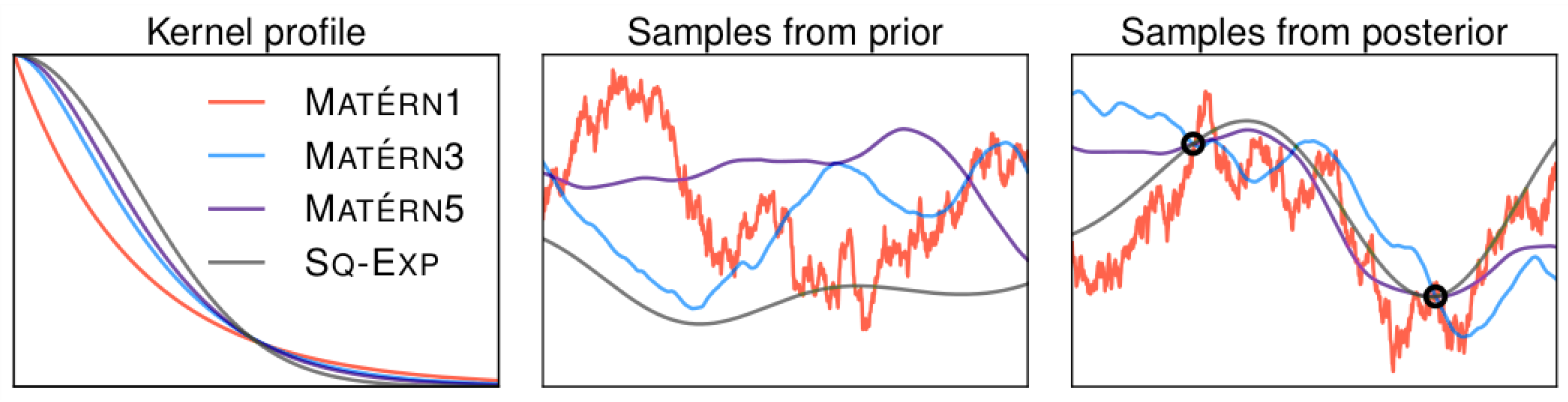
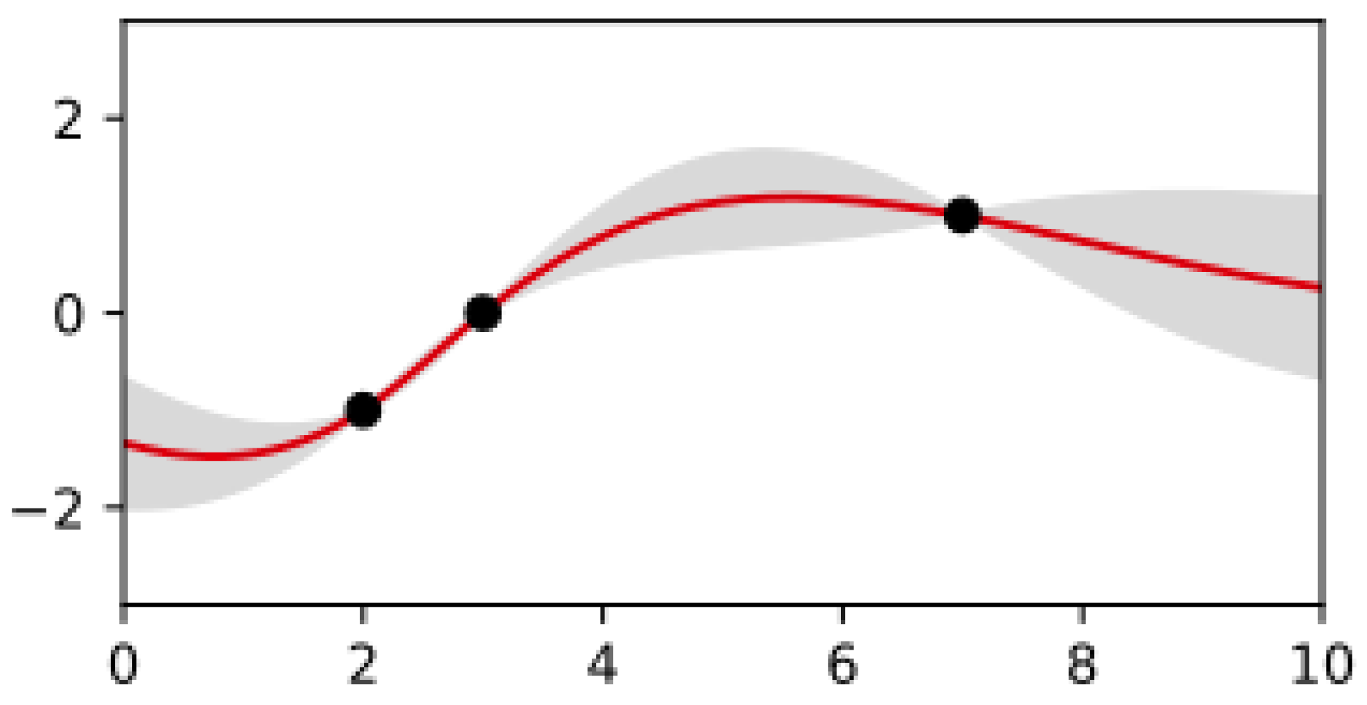
• The validation loss l is modeled as a Gaussian process (GP) f based on the assumption that two configurations $\lambda$ and ${\lambda }^{\prime }$ will perform similarly if they are similar according to some kernel $k(\lambda ,{\lambda }^{\prime })$. The Gaussian process f is used as a surrogate to estimate the expected value and variance of l given $\lambda$. Using Bayesian optimization l will be sampled at promising positions to iteratively improve f. Hyperparameter configurations that are expected to perform worse than the current optimum will not be sampled. This effectively reduces T.
• The optimizer is given an additional degree of freedom by modeling the training dataset size S as an additional hyperparameter of f. When trained on the whole dataset, this enables projecting the value of l while only probing smaller sections, thereby reducing the size of S.

We will now describe how those two ideas can be applied.

3.1.1. Gaussian Processes

A Gaussian process is a family of random variables (RVs) ${\left(X_{\theta }\right)}_{\theta \in \Theta }$, s. t. every finite subset of them follows a multivariate normal distribution. More intuitively it can be understood as a probability distribution over functions $f:\Theta \to \mathbb{R}$ where $X_{\theta }\widehat{=}f\left(\theta \right)$. Prior knowledge about the likelihood of each f is described by a prior mean function ${\mu }_0\left(\theta \right)=\mathbb{E}\left[f\left(\theta \right)\right]$ and a positive-definite kernel $k(\theta ,{\theta }^{\prime })=\mathrm{Cov}(f\left(\theta \right),f\left({\theta }^{\prime }\right))$. The covariance kernel models how informative it is to know $f\left(\theta \right)$ to determine $f\left({\theta }^{\prime }\right)$.

Let ${\mathcal{D}}_n={\left\{({\mathbf{\theta }}_i,{\mathit{y}}_i)\right\}}_{i=1}^n$ denote a set of observations. Those observations can be used to update the means and variances of the RVs via GP regression. This collapses the space of possible functions f to those functions that align with ${\mathcal{D}}_n$ (see Figure 1):

$$\begin{array}{cc}\hfill \mathit{m}:=& {({\mu }_0\left({\mathbf{\theta }}_1\right),\cdots ,{\mu }_0\left({\mathbf{\theta }}_n\right))}^T\hfill \\ \hfill \mathit{k}\left(\theta \right):=& {(k({\mathbf{\theta }}_1,\theta ),\cdots ,k({\mathbf{\theta }}_n,\theta ))}^T\hfill \\ \hfill \mathit{K}\in & {\mathbb{R}}^{n\times n}, {\mathit{K}}_{ij}:=k({\mathbf{\theta }}_i,{\mathbf{\theta }}_j)\hfill \end{array}$$

$$\begin{array}{cc}\hfill \mathbb{E}\left[f\left(\theta \right)\right|{\mathcal{D}}_n]:=& {\mu }_n\left(\theta \right)={\mu }_0\left(\theta \right)+\mathit{k}{\left(\theta \right)}^T{\mathit{K}}^{-1}(\mathit{y}-\mathit{m})\hfill \end{array}$$

(4)

$$\begin{array}{cc}\hfill \mathrm{Cov}(f\left(\theta \right),f\left({\theta }^{\prime }\right)|{\mathcal{D}}_n):=& k(\theta ,{\theta }^{\prime })-\mathit{k}{\left(\theta \right)}^T{\mathit{K}}^{-1}\mathit{k}\left({\theta }^{\prime }\right)\hfill \end{array}$$

(5)

Equation (4) can be extended to include an additional term that accounts for the uncertainty in the predictions, resulting in an alternative equation as in Equation (6).

$$\mathbb{E}[f\left(\theta \right),|,\mathcal{D}n]:={\mu }_n\left(\theta \right)={\mu }_0\left(\theta \right)+\mathit{k}{\left(\theta \right)}^T{\mathit{K}}^{-1}(\mathit{y}-\mathit{m})+\mathit{k}{\left(\theta \right)}^T{\mathit{K}}_{}^{-1}(\mathit{y}\ast -\mathit{m}\ast )$$

(6)

where $\mathit{k}\ast \left(\theta \right)$ is a vector of function evaluations at the point $\theta$ using the same kernel function as before, $\mathit{K}$ is the kernel matrix of the test points, ${\mathit{y}}_{}$ is the corresponding vector of function values at the test points, and ${\mathit{m}}_{\ast }$ is the corresponding vector of prior means at the test points.

Another alternative equation that can be used is the predictive distribution of the function at a new point $\theta$ given the observed data:

$$p(f\left(\theta \right),|,{\mathcal{D}}_n,\theta )=\mathcal{N}({\mu }_n\left(\theta \right),{\sigma }_n^2\left(\theta \right))$$

(7)

where $\mathcal{N}({\mu }_n\left(\theta \right),{\sigma }_n^2\left(\theta \right))$ is a Gaussian distribution with mean ${\mu }_n\left(\theta \right)$ and variance ${\sigma }_n^2\left(\theta \right)$ given by Equation (8).

$${\mu }_n\left(\theta \right)=\mathit{k}{\left(\theta \right)}^T{\mathit{K}}^{-1}\mathit{y}{\sigma }_n^2\left(\theta \right)=k(\theta ,\theta )-\mathit{k}{\left(\theta \right)}^T{\mathit{K}}^{-1}\mathit{k}\left(\theta \right)$$

(8)

The difference between Equations (6) and (7) is that the latter gives the probability distribution of the function value at a new point, given the data, rather than just the expected value. It is worth noting that when the kernel matrix is not invertible, one can use techniques such as regularization or a more expressive kernel function. Additionally, the above equations assume that the noise in the observations is Gaussian distributed, which is not always the case in practice.

Equation (5) can be also extended to calculate the joint posterior distribution of the function at multiple points. The joint posterior distribution of the function at a set of points $\Theta$ = ${\theta }_1$, ${\theta }_2$, …, ${\theta }_m$ is a multivariate Gaussian distribution with mean vector calculated as in Equation (9) and covariance matrix calculated as in Equation (10).

$$\mathbb{E}[f(\Theta ),|,{\mathcal{D}}_n]={\mu }_n(\Theta )={\mu }_0(\Theta )+\mathit{K}{(\Theta ,{\mathbf{\theta }}_1)}^T{\mathit{K}}^{-1}(\mathit{y}-\mathit{m})$$

(9)

$$\mathrm{Cov}(f(\Theta ),f(\Theta ),|,{\mathcal{D}}_n)=\mathit{K}(\Theta ,\Theta )-\mathit{K}{(\Theta ,{\mathbf{\theta }}_1)}^T{\mathit{K}}^{-1}\mathit{K}({\mathbf{\theta }}_1,\Theta )$$

(10)

where $\mathit{K}(\Theta ,{\mathbf{\theta }}_1)$ and $\mathit{K}({\mathbf{\theta }}_1,\Theta )$ are sub-matrices of the kernel matrix $\mathit{K}$ with elements $k({\theta }_i,{\mathbf{\theta }}_j)$ and $k({\mathbf{\theta }}_i,{\theta }_j)$ respectively, and $\mathit{K}(\Theta ,\Theta )$ is a sub-matrix of the kernel matrix with elements $k({\theta }_i,{\theta }_j)$.

Given this mean vector and covariance matrix, one can calculate any desired statistics of the function such as the probability of function values lying within a certain range or the expected value of a function at a particular point. It is also worth mentioning that the above equations assume that the kernel matrix is invertible, which is not always the case in practice, for instance when there is a linear dependence among the input points. To overcome this issue, one can use techniques like regularization, to make the matrix invertible.

Fabolas works by modeling the loss function l as a Gaussian process $f\sim \mathcal{GP}(m,k)$ with parameter set $\Theta :=\Lambda \times [0,1]$ where ${\mu }_0(\lambda ,s)=\mathbb{E}\left[f(\lambda ,s)\right]=\mathbb{E}\left[l\left(\lambda \right)\right|\mathrm{training}\mathrm{size}s]$. The product kernel that is being used in this case is a combination of two different kernel functions, one for the hyperparameters and one for the training set sizes. The kernel function for the hyperparameters is $k_{\mathrm{MATÉRN}5}\left(d_M(\lambda ,{\lambda }^{\prime })\right)$, where $d_M$ is a distance metric in the hyperparameter space and $k_{\mathrm{MATÉRN}5}$ is the Matérn 5/2 kernel function. The Matérn 5/2 kernel is a widely used kernel function in Gaussian process regression, it is a member of the Matérn family of kernels and it is characterized by a smoothness parameter and a length scale parameter. It allows the model to capture the smoothness of the underlying function in the hyperparameter space while also allowing for some flexibility. To model the covariances between different combinations of hyperparameters and training set sizes, the following product kernel is used:

$$\begin{array}{cc}\hfill k((\lambda ,s),({\lambda }^{\prime },s^{\prime })):=& k_{\mathrm{MATÉRN}5}\left(d_M(\lambda ,{\lambda }^{\prime })\right)·k_{\mathrm{lin}}(s,s^{\prime })\hfill \end{array}$$

(11)

Here $k_{\mathrm{MATÉRN}5}$ denotes the stationary Matérn kernel ($\nu =5/2$) with $d_M$ being the Mahalanobis distance between the two compared hyperparameter configurations. $k_{\mathrm{lin}}$ essentially is a simple linear kernel modeling the assumption that l monotonically decreases when s is increased. This product kernel allows the model to capture the interactions between the different dimensions of the parameter space (hyperparameters and training set sizes) while also preserving the ability to model the individual dimensions separately. The Matérn 5/2 kernel is used to model the smoothness of the underlying function in the hyperparameter space and the linear kernel is used to model the relationship between the training set sizes.

Equation (11) can be further extended by adding more kernel functions and combining them in different ways to better model the underlying function and its interactions in the parameter space. One alternative equation could be Equation (12).

$$\begin{array}{c}\hfill k((\lambda ,s),({\lambda }^{\prime },s^{\prime })):=k_{\mathrm{MATÉRN}5}\left(d_M(\lambda ,{\lambda }^{\prime })\right)\\ \hfill ·k_{\mathrm{lin}}(s,s^{\prime })+k_{\mathrm{RATIONALQUADRATIC}}\left(d_R(\lambda ,{\lambda }^{\prime })\right)\\ \hfill ·k_{\mathrm{Periodic}}(s,s^{\prime })\end{array}$$

(12)

The Equation (12) is using a combination of Matérn kernel, linear kernel, Rational Quadratic kernel, and a periodic kernel. The Matérn kernel captures the smoothness and the Rational Quadratic kernel allows for a more flexible model by allowing for different variances in different regions of the input space. The linear kernel models the linear relationship between the training set sizes, and the periodic kernel captures the periodicity of the underlying function in the training set size dimension. Another alternative extension could be Equation (13).

$$k((\lambda ,s),({\lambda }^{\prime },s^{\prime })):=k_{\mathrm{SE}}\left(d_E(\lambda ,{\lambda }^{\prime })\right)·k_{\mathrm{RBF}}(s,s^{\prime })$$

(13)

The Equation (13) is using a combination of Squared Exponential kernel and Radial Basis Function kernel. The SE kernel is a popular choice for GP models because it’s infinitely differentiable, and it’s able to model smooth functions. The RBF kernel is a versatile kernel that can capture a wide range of behaviors, it is defined as the exponentiation of the negative squared distance between two inputs. It is worth noting that the choice of kernel functions and their combination depends on the specific problem and assumptions made about the underlying function, the use of appropriate kernel functions and the combination of them can improve the performance of the model. We will now give an intuition for this choice of kernel and refer to Klein et al. [56] for the details. The Mahalanobis distance $d_M$ is used instead of the Euclidean distance because the hyperparameters in a configuration typically use very different scales and are in some cases also correlated.

Based on the Mahalanobis distance between two configurations $\lambda , {\lambda }^{\prime }$ the MATÉRN5 kernel is used to compute a covariance. The class of Matérn kernels interpolates between the Gaussian (SQ-EXP) and the exponential (MATÉRN1) kernel (see Figure 1). Because the exponential kernel drops off quickly, configurations quickly become uncorrelated which causes noisy samples. The Gaussian kernel drops off less quickly causing smoother samples. Fabolas uses MATÉRN5 as it empirically fits the smoothness of typical loss functions l quite well. Please refer to Schön et al. [57] for an explanation of why this is the case.

The product kernel of Equation (11) can be extended by incorporating the Mahalanobis distance, $\left(d_M\right)$ in the kernel functions. Hence, it can be written as in Equation (14).

$$k((\lambda ,s),({\lambda }^{\prime },s^{\prime })):=k_{\mathrm{SE}\text{-}\mathrm{MAHAL}}\left(d_M(\lambda ,{\lambda }^{\prime })\right)·k_{\mathrm{RBF}\text{-}\mathrm{MAHAL}}(s,s^{\prime })$$

(14)

where the Squared Exponential kernel is defined as in Equation (15).

$$k_{\mathrm{SE}\text{-}\mathrm{MAHAL}}\left(d_M(\lambda ,{\lambda }^{\prime })\right)=\exp \left(-\frac{1}{2}{d}_M{(\lambda ,{\lambda }^{\prime })}^2\right)$$

(15)

And the Radial Basis Function kernel is defined as in Equation (16).

$$k_{\mathrm{RBF}\text{-}\mathrm{MAHAL}}(s,s^{\prime })=\exp \left(-\frac{1}{2}{d}_M{(s,s^{\prime })}^2\right)$$

(16)

The Equation (16) is using a combination of Squared Exponential kernel and Radial Basis Function kernel where both of them are based on the Mahalanobis distance. The Mahalanobis distance is a measure of distance between two points in a multivariate space, it’s particularly useful when the data has correlations between features. An alternative equation could be as in Equation (17).

$$k((\lambda ,s),({\lambda }^{\prime },s^{\prime })):=k_{\mathrm{MATÉRNL}\text{-}\mathrm{MAHAL}}\left(d_M(\lambda ,{\lambda }^{\prime })\right)·k_{\mathrm{Periodic}\text{-}\mathrm{MAHAL}}(s,s^{\prime })$$

(17)

where the Matérn 1/2 kernel is defined as in Equation (18).

$$k_{\mathrm{MATÉRNL}\text{-}\mathrm{MAHAL}}\left(d_M(\lambda ,{\lambda }^{\prime })\right)=\frac{1}{2}(1+\sqrt{3}{d}_M(\lambda ,{\lambda }^{\prime }))\exp \left(-\sqrt{3}{d}_M(\lambda ,{\lambda }^{\prime })\right)$$

(18)

And the Periodic kernel is defined as in Equation (19)

$$k_{\mathrm{Periodic}\text{-}\mathrm{MAHAL}}(s,s^{\prime })=\exp \left(-2{sin}^2\left(\frac{\pi d_M(s,s^{\prime })}{p}\right)\right)$$

(19)

The Equation (19) is using a combination of Matérn 1/2 kernel, and Periodic kernel where both of which are based on the Mahalanobis distance. The Matérn 1/2 kernel is a member of the Matérn family of kernels and it’s characterized by a smoothness parameter, it allows for modeling functions with less smoothness than the Matérn 5/2 kernel, also the periodic kernel captures the periodicity of the underlying function in the training set size dimension based on the Mahalanobis distance.

3.1.2. Bayesian Optimization

To find $arg{min}_{\lambda }l\left(\lambda \right)$ the bias and variance of f have to be reduced by probing l at promising positions. This is called Bayesian optimization. The estimated minimum after n samples are described by $arg{min}_{\lambda }{\mu }_n(\lambda ,s=1)$, i.e., the configuration with the smallest predicted error on the full test dataset. To reduce the number of samples required until this minimum converges, an acquisition function is used. Its role is to trade-off exploration vs. exploitation of l by describing the expected utility of probing $({\lambda }_{n+1},s_{n+1})$ given a set of previous samples ${\mathcal{D}}_n$. Fabolas uses an aquisition function that rates configurations by their information gain per computation time:

$$\begin{array}{cc}\hfill a_F(\lambda ,s):=& \frac{1}{c(\lambda ,s)}{\mathbb{E}}_y\left[p\left(y\right|\lambda ,s,{\mathcal{D}}_n)·{\mathrm{KL}}_{\widehat{\lambda }}(p_{min}\left(\widehat{\lambda }\right|{\mathcal{D}}_n\cup \left\{(\lambda ,s,y)\right\})\parallel u\left(\widehat{\lambda }\right))\right]\hfill \\ \hfill p_{min}\left(\lambda \right|\mathcal{D}):=& p(\lambda \in arg\underset{{\lambda }^{\prime }}{min}f({\lambda }^{\prime },s=1)|\mathcal{D})\hfill \end{array}$$

(20)

Based on the Kullback-Leibler (KL) of Equation (20), the promising position according to $a_F$ is as shown in Figure 2. KL divergence, also known as relative entropy, is a measure of the difference between two probability distributions. It measures how much information is lost when approximating one distribution with another.

Equation (20) is using the expected value of the probability of observing the loss value y at configuration $(\lambda ,s)$ given the previous samples ${\mathcal{D}}_n$ and subtracting from it a term that represents the variance of the probability of observing the loss value y. This term is multiplied by a trade-off parameter $\beta$. This acquisition function is trying to balance the exploration and exploitation by emphasizing the configurations that have low variance in their predicted loss value. An alternative representation could be as in Equation (21).

$$a_F(\lambda ,s):=\frac{1}{c(\lambda ,s)}\mathbb{E}y\left[{\left(p(y,|,\lambda ,s,\mathcal{D}n)\right)}^2·\mathrm{KL}\widehat{\lambda }(pmin(\widehat{\lambda },|,{\mathcal{D}}_n\cup (\lambda ,s,y)),|,u\left(\widehat{\lambda }\right))\right]$$

(21)

Equation (21) is using the square of the probability of observing the loss value y at configuration $(\lambda ,s)$ given the previous samples ${\mathcal{D}}_n$ and multiplying it with the KL divergence term. This acquisition function is trying to balance the exploration and exploitation by emphasizing the configurations that have low loss values and high information gain. An alternative representation could be as in Equation (22).

$$a_F(\lambda ,s):=\frac{1}{c(\lambda ,s)}{\mathbb{E}}_y\left[{\left(p(y,|,\lambda ,s,{\mathcal{D}}_n)\right)}^2·\mathrm{UCB}(\lambda ,s)\right]$$

(22)

where $\mathrm{UCB}(\lambda ,s)$ is the Upper Confidence Bound of the expected loss value at configuration $(\lambda ,s)$. This acquisition function is trying to balance the exploration and exploitation by emphasizing the configurations that have low loss values and high upper bound of expected loss values. This can also be expressed as in Equation (23).

$$a_F(\lambda ,s):=\frac{1}{c(\lambda ,s)}\left[{\mathbb{E}}_y\left[p(y,|,\lambda ,s,{\mathcal{D}}_n)\right]-\beta ·{\mathrm{Entropy}}_y\left[p(y,|,\lambda ,s,{\mathcal{D}}_n)\right]\right]$$

(23)

where ${\mathrm{Entropy}}_y\left[p(y,|,\lambda ,s,{\mathcal{D}}_n)\right]$ is the entropy of the probability of observing the loss value y at configuration $(\lambda ,s)$ given the previous samples ${\mathcal{D}}_n$. This equation is using the expected value of the probability of observing the loss value y at configuration $(\lambda ,s)$ given the previous samples ${\mathcal{D}}_n$ and subtracting from it a term that represents the entropy of the probability of observing the loss value y. This term is multiplied by a trade-off parameter $\beta$. This acquisition function is trying to balance the exploration and exploitation by emphasizing the configurations that have low entropy in their predicted loss value.

Solving for ${\mathbb{E}}_y\left[p(y,|,\lambda ,s,{\mathcal{D}}_n)\right]$ in the acquisition function of Equation (21) requires knowledge of the underlying probability distribution of the loss value y given the configuration $(\lambda ,s)$ and the previous samples ${\mathcal{D}}_n$. Depending on the specific problem and assumptions made about the underlying function, different probability distributions can be used. An approximation of ${\mathbb{E}}_y\left[p(y,|,\lambda ,s,{\mathcal{D}}_n)\right]$ could be as in Equation (24).

$${\mathbb{E}}_y\left[p(y,|,\lambda ,s,{\mathcal{D}}_n)\right]={\mathbb{E}}_y\left[N(y,|,{\mu }_n(\lambda ,s),{\sigma }_n^2(\lambda ,s))\right]$$

(24)

where $N(y,|,{\mu }_n(\lambda ,s),{\sigma }_n^2(\lambda ,s))$ is the normal distribution with mean ${\mu }_n(\lambda ,s)$ and variance ${\sigma }_n^2(\lambda ,s)$. This equation assumes that the loss value y follows a normal distribution given the configuration $(\lambda ,s)$ and the previous samples ${\mathcal{D}}_n$. Another approximation could be as in Equation (25).

$${\mathbb{E}}_y\left[p(y,|,\lambda ,s,{\mathcal{D}}_n)\right]={\mathbb{E}}_y\left[U(y,|,a_n(\lambda ,s),b_n(\lambda ,s))\right]$$

(25)

where $U(y,|,a_n(\lambda ,s),b_n(\lambda ,s))$ is the uniform distribution with lower bound $a_n(\lambda ,s)$ and upper bound $b_n(\lambda ,s)$. This equation assumes that the loss value y follows a uniform distribution given the configuration $(\lambda ,s)$ and the previous samples ${\mathcal{D}}_n$.

Since it is infeasible to compute $a_F$ numerically, its maximum is estimated using Markov-Chain Monte Carlo (MCMC). As with other Monte Carlo approaches, MCMC exploits the law of large numbers via repeated random sampling. Samples are produced by executing a Markov Chain whose stationary distribution is designed to match the input function, for which a proposal distribution is used [58]. One popular variation of MCMC is distributed Gibbs sampling, which allows for parallelization and improves computational efficiency [59]. This method may be used for optimization tasks, approximating solutions to non-deterministic polynomial time problems, and bayesian optimizations. Maximum likelihood estimation can also be performed using MCMC methods to estimate the model parameters [60]. The estimated most promising configuration will be sampled. The resulting loss value and runtime are then used to update the loss model f and cost model c via GP regression.

3.2. Simulation Interface and Datasets

3.2.1. Simulation Interface

The simulations presented in Section 3.2.3, Section 3.3.2, Section 4.1.2, Section 4.2.2, Section 4.3.4 and Section 4.4.1 are all under the same Hardware, Software, and Setup. The specific configurations are shown in

Table 1. Simulation Interface Components.

CPU	Memory	Programming Language	Operating System
i9-10850k	32GB	Python 3.10	Windows 11

.

3.2.2. Datasets

For the evaluation of Fabolas, Bag of Little Bootstraps (BLB), Local Case-Control (LCC), OSMAC, KM-SVM, and WKM-SVM different datasets are used. These are summarized in

Table 2. Dataset information for each method and the number of samples contained in it.

Dataset	Evaluation for Method	No. of Samples
CIFAR-10	Fabolas	60,000
MNIST	Fabolas	70,000
Randomly Generated	BLB	20,000
Randomly Generated	OSMAC	10,000
PimaIndiansDiabetes2	KM-SVM and WKM-SVM	768

.

3.2.3. Evaluation

Fabolas was evaluated in support vector machine (SVM) and convolutional neural network (CNN) optimization tasks on the MNIST and CIFAR-10 dataset respectively. Figure 3 compares Fabolas (The average over 10 runs are depicted) to the following other hyperparameter optimization approaches:

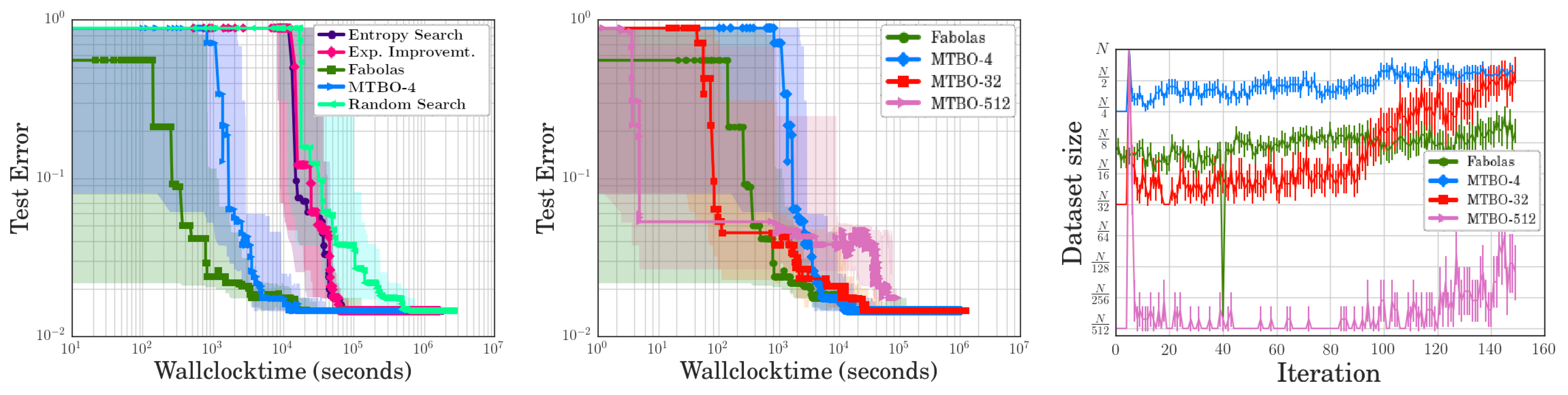
• Random Search: Simple random hyperparameter search. Each configuration is evaluated on the full dataset.
• Entropy Search & Expected Improvement: Bayesian optimization methods always evaluate the full dataset. Expected Improvement uses an acquisition function that simply samples at the current expected optimum. Entropy Search uses an acquisition function similar to the one used by Fabolas but without the cost model.
• MTBO-N (Multi-Task Bayesian Optimization [61]): Like Fabolas but restricts samples to two sizes $s\in \{1/N,1\}$, i.e., either a small subsample or the entire dataset is used. Multiple values for N are evaluated: 4, 32, and 512.

Random search is at least one order of magnitude slower than any Bayesian optimization technique. Two probing sizes are supported by MTBO, which makes it an additional order of magnitude quicker. Depending on the choice of N, MTBO occasionally advances more quickly than Fabolas at first. Fabolas does, however, locate a suitable configuration somewhat more quickly than MTBO once it begins to advance. Both Fabolas and MTBO discover the ideal arrangement at around the same time. In comparison to random search, Fabolas identifies a suitable configuration between 100 and 1000 times quicker. When CNNs are optimized using CIFAR-10, similar outcomes are found.

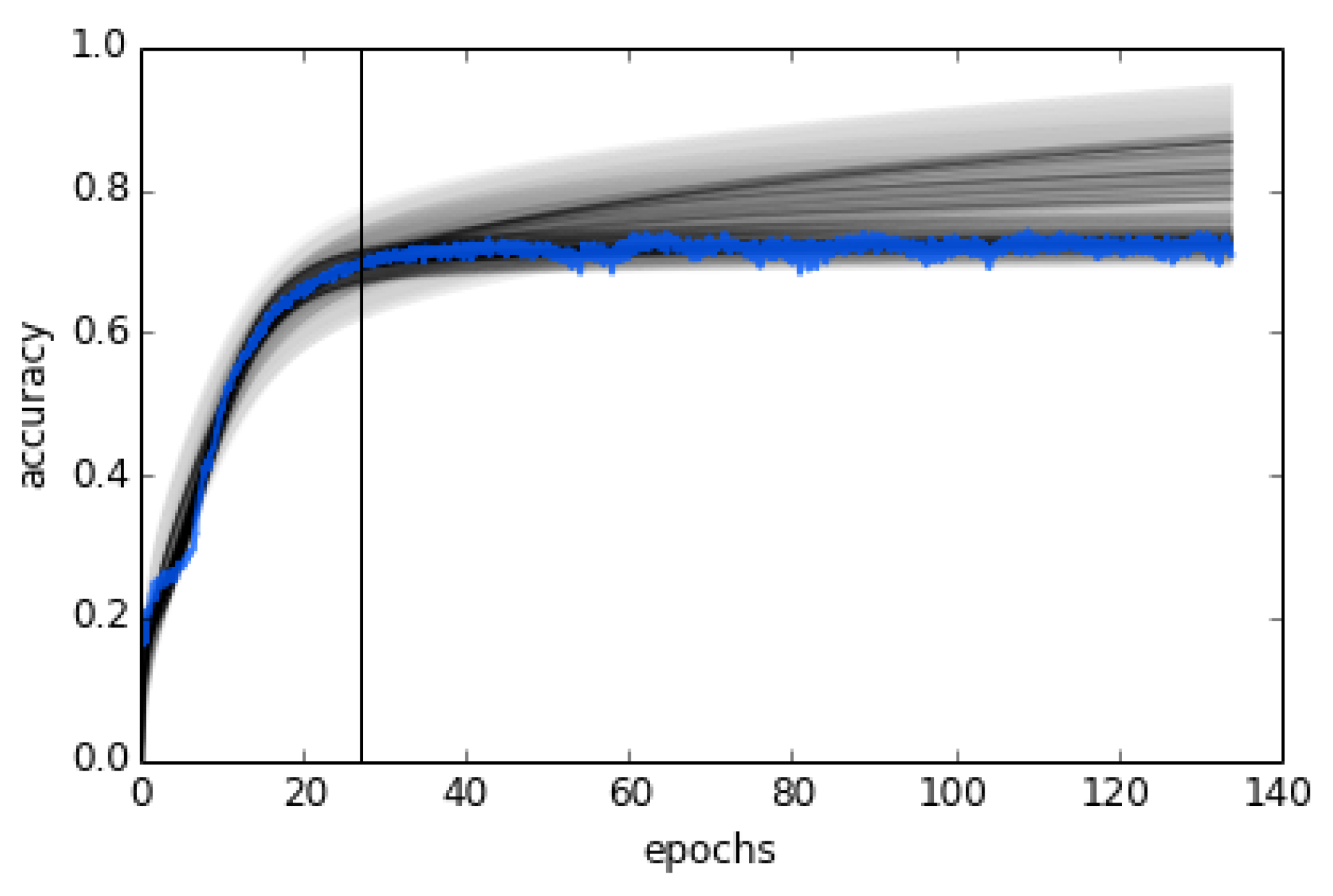
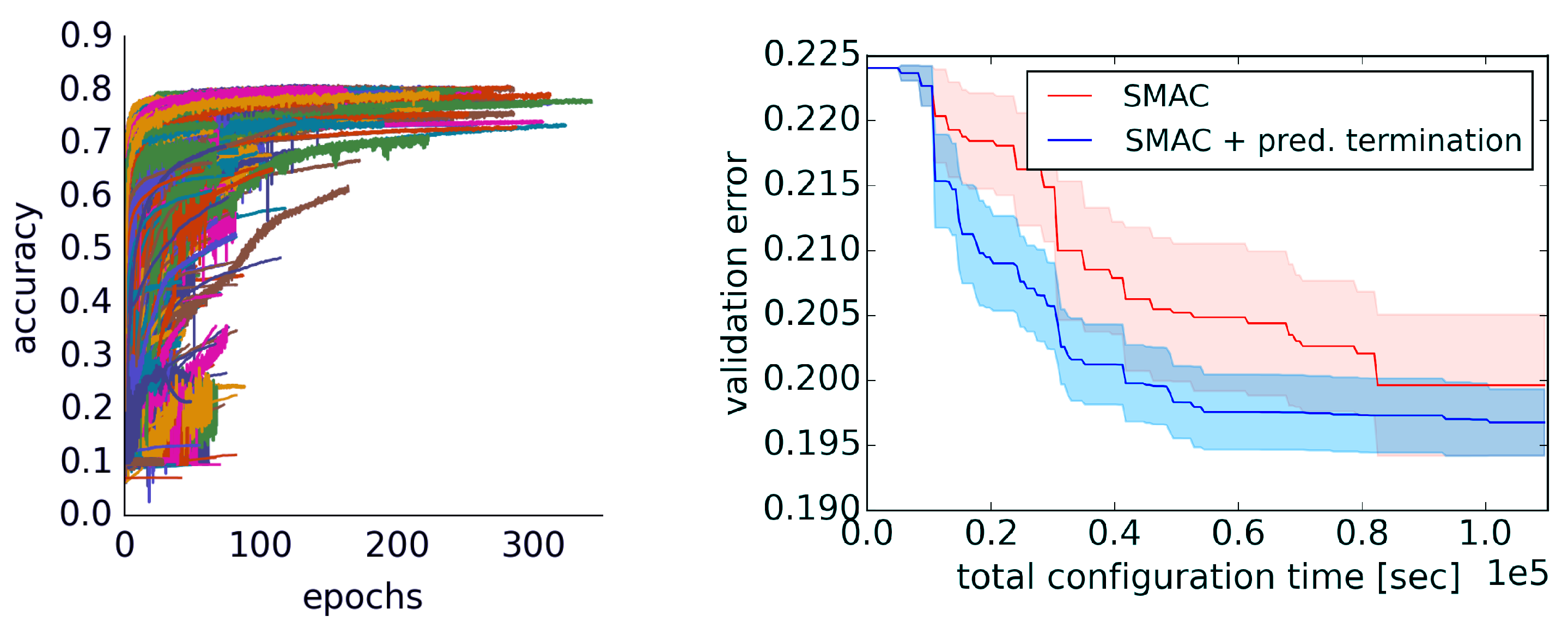
3.3. Learning Curve Extrapolation

Reduced training iterations E are the main goal of the second strategy for accelerating hyperparameter tuning. It may theoretically be incorporated into any hyperparameter optimizer and applied to any gradient descent-based learner. The goal is to use a hyperparameter configuration called $\lambda$ to track a learner’s learning curve as they progress through training. Training will end before convergence if it is doubtful that a good accuracy will be achieved with $\lambda$.

The method was first described by Domhan et al. [62] in the context of hyperparameter optimization for deep neural networks (DNNs) that are trained using stochastic gradient descent (SGD). Since no strong assumptions specific to DNNs are made, it can however also be used for other learners. DNNs were used because their gradient descent steps are comparatively expensive.

3.3.1. Extrapolation Method

Let $y_{1:n}$ denote the observed learning curve of SGD after n iterations, i.e., the sequence of training accuracies $y_i\in [0,1]$. Normally SGD iterations would be run for each hyperparameter configuration $\lambda$ until convergence or until a maximum number of iterations E has been reached. The learning curve extrapolation optimization works by predicting $y_E$ every p iteration. This is further shown in Algorithm 1.

Algorithm 1: Extrapolation Method.

1: $\widehat{y}\leftarrow -\infty$ 2: for $\lambda \leftarrow$ next hyperparameter configuration to evaluate do 3:     $n\leftarrow 0$ 4:     repeat 5:         Run p SGD iterations using $\lambda$ with resulting accuracies $y_{(n+1):(n+p)}$. 6:         $n\leftarrow n+p$ 7:         Estimate $P(y_E<\widehat{y}|y_{1:n})$. 8:     until $\mathrm{SGD}\mathrm{converged}\vee n\ge E\vee P(y_E<\widehat{y}|y_{1:n})>\delta$ 9:     if $y_n>\widehat{y}$ then $\widehat{y}\leftarrow y_n$ end if 10: end for

Algorithm 1 starts by initializing the best accuracy achieved so far, represented by the variable $\widehat{y}$, to the lowest possible value ($-\infty$). The algorithm then iterates over the next hyperparameter configuration to evaluate. For each configuration, the algorithm initializes a counter variable n to 0 and enters a loop. In each iteration of the loop, the algorithm runs p SGD iterations using the current hyperparameter configuration and records the resulting accuracy in the set $y_{(n+1):(n+p)}$. The counter variable n is incremented by p. The algorithm then estimates the probability $P(y_E<\widehat{y},|,y_{1:n})$ (Line 6) of the model achieving better accuracy than the best accuracy achieved so far, given the accuracy values observed so far. The loop continues until either SGD converged, the number of iterations reaches a maximum value of E, or the estimated probability of achieving better accuracy than the best accuracy achieved so far is greater than a threshold value $\delta$. If the accuracy of the current iteration $y_n$ is greater than the best accuracy achieved so far $\widehat{y}$, the algorithm updates the value of $\widehat{y}$ with the current accuracy value $y_n$. After evaluating all the hyperparameter configurations, the algorithm returns the best accuracy achieved so far, represented by the variable $\widehat{y}$.

The prediction step (line 7) uses a probabilistic model. Similar to Fabolas, a distribution over candidate functions is fitted to the observations $y_{1:n}$. Unlike Fabolas however, which uses a flexible non-parametric GP model, we use prior knowledge about the shape of learning curves to restrict the model to parameterized, increasing, and saturating functions. More specifically, the learning curve $y_{1:n}$ is modeled as a linear combination $f_{\mathit{comb}}$ of a family of given functions.

$$\begin{array}{cc}\hfill f_{\mathit{comb}}\left(t\right|\xi ):=& \sum _{k=1}^K{w}_k{f}_k\left(t\right|{\theta }_k),\xi =(w_1,\cdots ,w_k,{\theta }_1,\cdots ,{\theta }_k,{\sigma }^2)\hfill \end{array}$$

(26)

$$\begin{array}{cc}\hfill y_t\sim & \mathcal{N}(f_{\mathit{comb}}\left(t\right|\xi ),{\sigma }^2)\hfill \end{array}$$

(27)

Domhan et al. [62] use $K=11$ types of functions $\{f_1,\cdots ,f_K\}$ that are each parameterized by $\{{\theta }_1,\cdots ,{\theta }_K\}$. Equation (26) can also be modeled as in Equation (28) which includes additional terms to the linear combination.

$$f_{\mathit{comb}}(t,|,\xi ):=\sum _{k=1}^K{w}_k{f}_k(t,|,{\theta }_k)+w_{K+1}{t}^2+w_{K+2}sin\left(t\right)$$

(28)

Or we can use a different probability distribution for the noise, such as a Student-t distribution instead of the normal distribution. This could be useful if the observations have heavier tails. It is also possible to include regularization terms in the model, such as L1 or L2 regularization, to prevent overfitting and to obtain more robust estimates of the model parameters. This is further shown in Equation (29).

$$f_{\mathit{comb}}(t,|,\xi ):=\sum _{k=1}^K{w}_k{f}_k(t,|,{\theta }_k)+\lambda \sum _{k=1}^K\left|w_k\right|$$

(29)

Another alternative is to use a more complex model for the learning curve, such as a neural network. This could allow for more flexibility in modeling the underlying function, but also requires more data and more computational resources to train. This is further shown in Equation (30).

$$f_{\mathit{comb}}(t,|,\xi ):=NeuralNetwork(t,\theta )$$

(30)

where $NeuralNetwork$ is a deep neural network with parameter set $\theta$.

Figure 4 shows the best accuracy achieved by Algorithm 1. The assumption is that every function type captures certain aspects of learning curves. By allowing linear combinations a more powerful model can be obtained. Figure 5 illustrates this idea.

As can be seen in the legend on the left, the linear combination has the smallest deviation $\Delta y$ from the observed data after 300 iterations. To estimate the probability $P(y_E<\widehat{y}|y_{1:n})$ MCMC is used to sample S learning curves $\{{\xi }_1,\cdots ,{\xi }_S\}$ from the posterior:

$$\begin{array}{cc}\hfill P\left(\xi \right|y_{1:n})\propto & P\left(y_{1:n}\right|\xi )P\left(\xi \right)\hfill \end{array}$$

(31)

$$\begin{array}{cc}\hfill P\left(y_{1:n}\right|\xi )=& \prod _{t=1}^n\mathcal{N}(y_t;f_{\mathit{comb}}\left(t\right|\xi ),{\sigma }^2)\hfill \end{array}$$

(32)

$$\begin{array}{cc}\hfill P\left(\xi \right)\propto & \mathbb{1}[f_{\mathit{comb}}\left(1\right|\xi )<f_{\mathit{comb}}\left(E\right|\xi )\wedge \forall k:w_k>0]\hfill \end{array}$$

(33)

From Equation (31) we can define $P\left(\xi \right)$ using a prior distribution on the parameters, such as a normal distribution for the weights and a uniform distribution for the parameters of each function type. An example is given in Equation (34).

$$P\left(w_k\right)=\mathcal{N}(w_k;0,1)P\left({\theta }_k\right)=\mathrm{Uniform}({\theta }_k;{\theta }_{k,\min },{\theta }_{k,\max })P\left({\sigma }^2\right)=\mathrm{Inv}\text{-}\mathrm{Gamma}({\sigma }^2;a,b)$$

(34)

where $P\left(w_k\right),P\left({\theta }_k\right)$ and $P\left({\sigma }^2\right)$ are the prior distributions for the weights, function parameters, and variance respectively. Another alternative is to use a non-informative prior like Jeffreys prior, which is the square root of the determinant of the Fisher information matrix. This is further shown in Equation (35).

$$P\left(w_k\right)=\frac{1}{\sqrt{I\left(w_k\right)}},P\left({\theta }_k\right)=\frac{1}{\sqrt{I\left({\theta }_k\right)}},P\left({\sigma }^2\right)=\frac{1}{\sqrt{I\left({\sigma }^2\right)}}$$

(35)

where $I\left(w_k\right),I\left({\theta }_k\right)$ and $I\left({\sigma }^2\right)$ are the Fisher information for the respective parameter. The prior $P\left(\xi \right)$ is used to model the fact that learning curves do not typically decrease over time. Given the learning curve samples, we can now estimate from Equation (31) the following.

$$\begin{array}{cc}\hfill P(y_E<\widehat{y}|y_{1:n})=& \int P\left(\xi \right|y_{1:n})P(y_E<\widehat{y}|\xi )\mathrm{d}\xi \hfill \\ \hfill \approx & \frac{1}{S}\sum _{s=1}^S\Phi (\widehat{y};f_{\mathit{comb}}\left(E\right|{\xi }_s),{\sigma }^2)\hfill \end{array}$$

(36)

Alternatively, the prior $P\left(\xi \right)$ can be modeled as a hierarchical prior with a hierarchical structure for the weights w and the parameters $\theta$.

$$\begin{array}{cccc}\hfill P\left(\xi \right)\propto & \prod _{k=1}^{K}P\left(w_k\right)P\left({\theta }_k\right)P\left(w_k\right)\propto \hfill & \hfill \mathrm{Gamma}\left(w_k\right|a,b)P\left({\theta }_k\right)\propto & \mathrm{Normal}\left({\theta }_k\right|\mu ,\sigma )\hfill \end{array}$$

(37)

This allows for more control over the shape of the prior for the weights and parameters and can help encourage certain properties, such as sparsity in the weights. Additionally, instead of using MCMC for sampling from the posterior, other methods such as Variational Inference or Hamiltonian Monte Carlo can be used for faster and more efficient sampling.

An alternative equation for $P\left(w_k\right)$ could be a Dirichlet distribution, which is a multivariate generalization of the Gamma distribution.

$$P\left(w_k\right)\propto \mathrm{Dirichlet}\left(w_k\right|{\alpha }_1,\cdots ,{\alpha }_K)$$

(38)

Another alternative equation for $P\left({\theta }_k\right)$ could be a Laplace distribution, which is a continuous probability distribution that is similar to the normal distribution but has heavier tails.

$$P\left({\theta }_k\right)\propto \mathrm{Laplace}\left({\theta }_k\right|\mu ,b)$$

(39)

Additionally, other alternatives for $P\left({\theta }_k\right)$ could be a Student-t distribution or a Cauchy distribution, which are both distributions with heavy tails and can be used to model outliers in the data.

$$P\left({\theta }_k\right)\propto \mathrm{Student}\text{-}\mathrm{t}\left({\theta }_k\right|\mu ,\sigma ,\nu )orP\left({\theta }_k\right)\propto \mathrm{Cauchy}\left({\theta }_k\right|\mu ,\sigma )$$

(40)

For Variational Inference, one could use a mean-field approximation to approximate the true posterior $\left(P\left(\xi \right|y_{1:n})\right)$ with a simpler family of distributions $\left(q\right(\xi \left)\right)$ that are easy to optimize. One would optimize the evidence lower bound (ELBO) of the log marginal likelihood $\left(logP\left(y_{1:n}\right)\right)$ using gradient-based optimization methods such as stochastic gradient descent. For Hamiltonian Monte Carlo, one could use the Metropolis-Hastings algorithm or the No-U-Turn Sampler to obtain samples from the true posterior $\left(P\left(\xi \right|y_{1:n})\right)$ by constructing a Markov chain that has the desired distribution as its stationary distribution. This method uses gradient information of the log-posterior to guide the proposal distribution and improve the efficiency of the sampling process.

For Variational Inference, the prior $\left(P\right(\xi \left)\right)$ is approximated by a simpler distribution $\left(Q\right(\xi \left)\right)$ that is easier to manipulate. The goal is to find the (Q) that minimizes the Kullback-Leibler divergence between (Q) and (P), which is equivalent to maximizing the Evidence Lower Bound (ELBO):

$$ELBO=\int Q\left(\xi \right)log\frac{P\left(\xi \mid y_{1:n}\right)}{Q\left(\xi \right)}d\xi =EQ\left(\xi \right)[logP(\xi \mid y1:n)]-KL\left(Q\left(\xi \right)\right|\left|P\left(\xi \right)\right)$$

(41)

For Hamiltonian Monte Carlo, the prior $\left(P\right(\xi \left)\right)$ is sampled using a Markov Chain Monte Carlo (MCMC) method. In HMC, a fictitious “momentum” variable is introduced and the sampling is done using Hamiltonian dynamics. This allows for more efficient exploration of the parameter space and can avoid getting stuck in local optima. The equations for updating the position and momentum variables at each iteration are as follows:

$$\begin{array}{cccc}\hfill p^{\left(i\right)}& \sim \mathcal{N}(0,m){\xi }^{(i+1/2)}\hfill & \hfill ={\xi }^{\left(i\right)}+\frac{ϵ}{2}{p}^{\left(i\right)}{p}^{(i+1)}& =\hfill \\ & p^{\left(i\right)}-ϵ{\nabla }_{\xi }logP\left({\xi }^{(i+1/2)}\right){\xi }^{(i+1)}\hfill & \hfill ={\xi }^{(i+1/2)}+\frac{ϵ}{2}{p}^{(i+1)}\end{array}$$

(42)

where $\left(p\right)$ is the momentum variable, $\left(m\right)$ is the mass matrix, and $\left(ϵ\right)$ is the step size.

For Hamiltonian Monte Carlo, the first step is to define the target distribution $\left(P\left(\xi \right|y_{1:n})\right)$ which is the posterior distribution that we want to sample from. We can then define a proposal distribution $\left(Q\left({\xi }^{\prime }\right|\xi )\right)$ which is used to generate new samples. The Metropolis-Hastings algorithm is then used to accept or reject new samples based on the acceptance probability:

$$\begin{array}{c}\hfill A(\xi \to {\xi }^{\prime })=\min \left[1,\frac{P\left({\xi }^{\prime }\right|y_{1:n})Q\left(\xi \right|{\xi }^{\prime })}{P\left(\xi \right|y_{1:n})Q\left({\xi }^{\prime }\right|\xi )}\right]\end{array}$$

(43)

In Hamiltonian Monte Carlo, the proposal distribution is defined based on the gradient of the target distribution, and the algorithm makes use of Hamiltonian dynamics to generate samples. The Hamiltonian dynamics are defined by the Hamiltonian function $\left(H\right(\xi ,p\left)\right)$ which is a combination of the potential energy $(U\left(\xi \right)=-logP\left(\xi \right|y_{1:n}))$ and the kinetic energy $(K\left(p\right)=\frac{1}{2}{p}^{T}p)$. The Hamiltonian dynamics are governed by Hamilton’s equations:

$$\begin{array}{c}\hfill \frac{d\xi }{dt}=\frac{\partial H}{\partial p}\mathrm{and}\frac{dp}{dt}=-\frac{\partial H}{\partial \xi }\end{array}$$

(44)

The algorithm then proceeds by initializing the position and momentum, and using the Hamiltonian dynamics to generate new samples. The acceptance probability is defined as

$$\begin{array}{c}\hfill A(\xi \to {\xi }^{\prime })=\min \left[1,e^{-\Delta H}\right]\end{array}$$

(45)

where $\Delta H$ is the change in the Hamiltonian between the current and proposed states.

3.3.2. Evaluation

The CIFAR-10, CIFAR-100, and MNIST datasets were used to assess the early termination strategy that we just discussed. The behavior of early termination and the speedup obtained on CIFAR-10 are shown in Figure 6. As anticipated, early termination occurs for setups with learning curves that have the propensity to approach low accuracies. High-accuracy configurations are tested till convergence. Across the studied datasets, our method consistently doubles the speed of the hyperparameter optimization while maintaining the same level of quality.

3.4. Fine-Tuning

In this subsection, we propose fine-tuning algorithmic schemes on what we have seen already. Below, we present Algorithm 2 which is an optimized version of Algorithm 1.

Algorithm 2: Extrapolation Method Optimized.

Require:  p, E, $\delta$ Ensure:  best_acc 1: best_acc $\leftarrow -\infty$ 2: for  $\lambda \in \mathrm{next}\_\mathrm{hyperparameter}\_\mathrm{configuration}()$  do 3:     $n\leftarrow 0$ 4:     while True do 5:         run_p_SGD_iterations ($\lambda$) 6:         $n\leftarrow n+p$ 7:         estimate_prob_better_acc(best_acc, y) 8:         if SGD_converged() or $n\ge E$ or prob_better_acc $>\delta$ then 9:            break 10:         end if 11:     end while 12:     if current_acc > best_acc then 13:         best_acc ← current_acc 14:     end if 15: end for 16: return best_acc

This version of the algorithm uses a function $next\_hyperparameter\_configuration\left(\right)$ to generate the next hyperparameter configuration for evaluation. The following function $run\_p\_SGD\_iterations\left(\lambda \right)$ runs the specified number of SGD iterations using the current hyperparameter configuration and records the resulting accuracy. The function $estimate\_prob\_better\_acc(best\_acc,y)$ estimates the probability of achieving better accuracy than the current best accuracy. The function $SGD\_converged\left(\right)$ checks if the training has converged. If the current accuracy is greater than the best accuracy so far, the best accuracy is updated.

However, we can further optimize the algorithm by running it in a parallel way. This is shown in Algorithm 3.

Algorithm 3: Extrapolation Method Optimized (Parallel).

1: import multiprocessing.Pool Require:  p, E, $\delta$, num_processes Ensure:  best_acc 2: best_acc $\leftarrow -\infty$ 3: $pool\leftarrow$ Pool(num_processes) 4: for$\lambda \in \mathrm{next}\_\mathrm{hyperparameter}\_\mathrm{configuration}()$  do 5:     $n\leftarrow 0$ 6:     while True do 7:         accs ← pool.map(run_p_SGD_iterations, [$\lambda$] * p) 8:         $n\leftarrow n+p$ 9:         estimate_prob_better_acc(best_acc, accs) 10:         if SGD_converged() or $n\ge E$ or prob_better_acc $>\delta$ then 11:            break 12:         end if 13:     end while 14:     if max(accs) > best_acc then 15:         best_acc ← max(accs) 16:     end if 17: end for 18: $pool.close\left(\right)$ 19: $pool.join\left(\right)$ 20: return best_acc

This version of the algorithm uses the multiprocessing library to parallelize the evaluation of different hyperparameter configurations. A Pool of worker processes is created with the specified number of processes. The $map\left(\right)$ function is used to apply the $run\_p\_SGD\_iterations$ function to a list of lambda values in parallel, and the resulting accuracy values are collected in a list accs.

Another hyperparameter optimization that utilizes simple gradient descent is shown in Algorithm 4.

Algorithm 4: Gradient Descent.

Require:  $\alpha$, max_iter, $\lambda$ Ensure:  $\lambda$ 1: $n\leftarrow 0$ 2: while $n<$ max_iter do 3:     grad ← compute_gradient($\lambda$) 4:     $\lambda \leftarrow \lambda -\alpha \times$ grad 5:     $n\leftarrow n+1$ 6: end while 7: return $\lambda$

This algorithm takes in three parameters: the learning rate alpha, the maximum number of iterations $max\_iter$, and the current hyperparameter configuration $\lambda$. In each iteration, the gradient of the loss function with respect to the hyperparameters is computed using the $compute\_gradient\left(\right)$ function, and the hyperparameters are updated in the direction of the negative gradient by subtracting $\alpha \times grad$ from the current configuration. The optimization process stops once the maximum number of iterations is reached, and the final hyperparameter configuration is returned. Algorithm 4 can be incorporated with Adaptive Moment Estimation (ADAM) optimizer which leads to Algorithm 5.

Algorithm 5: Adaptive Stochastic Gradient Descent.

Require:  $\alpha$, max_iter, $\lambda$, ${\beta }_1$ = 0.9, ${\beta }_2$ = 0.999, $ϵ$ = 1 × 10${}^{-8}$ Ensure:  $\lambda$ 1: $n\leftarrow 0$, $m\leftarrow 0$, $v\leftarrow 0$ 2: while $n<$ max_iter do 3:     grad ← compute_gradient($\lambda$) 4:     $n\leftarrow n+1$ 5:     $m\leftarrow {\beta }_1\times m+(1-{\beta }_1)\times grad$ 6:     $v\leftarrow {\beta }_2\times v+(1-{\beta }_2)\times (grad\times grad)$ 7:     $m\_hat\leftarrow m/(1-{\beta }_1^n)$ 8:     $v\_hat\leftarrow v/(1-{\beta }_2^n)$ 9:     $\lambda \leftarrow \lambda -\alpha \times m\_hat/(\sqrt{v\_hat}+ϵ)$ 10: end while 11: return $\lambda$

This algorithm also takes in three parameters: the learning rate alpha, the maximum number of iterations $max\_iter$, and the current hyperparameter configuration $\lambda$. In addition to that, the algorithm also takes in three other parameters that are the defaults for the Adam optimizer: ${\beta }_1$, ${\beta }_2$, and $ϵ$. In each iteration, the gradient of the loss function with respect to the hyperparameters is computed using the $compute\_gradient\left(\right)$ function, and the Adam optimizer updates the hyperparameters using the moving averages of the gradient and the squared gradient as well as the learning rate. Similar to Adam optimization algorithm, Adagrad, and RMSprop are also optimization algorithms that can be used to optimize the hyperparameters, they also have their own set of hyperparameters to tweak and fine-tune the optimization process, and the implementation of these algorithms can be found in their respective papers or in common deep learning libraries.

Next, we present an Algorithm for hyperparameter optimization in Apache Spark. This is further shown in Listing 1.

Listing 1: PySpark Linear Regression Cross-Validation.

import pyspark.ml.tuning.CrossValidator import pyspark.ml.evaluation.RegressionEvaluator import pyspark.ml.regression.LinearRegression import pyspark.ml.feature.VectorAssembler

df = spark.read.csv("path/to/data.csv", header=True) assembler = VectorAssembler(inputCols=["col1", "col2", "col3"], outputCol="features")

lr = LinearRegression()

paramGrid = ParamGridBuilder() .addGrid(lr.regParam, [0.1, 0.01, 0.001]) .addGrid(lr.fitIntercept, [False, True]) .build()

cv = CrossValidator(estimator = lr, estimatorParamMaps = paramGrid, evaluator = RegressionEvaluator(), numFolds = 5)

cvModel = cv.fit(df)

This algorithm uses the CrossValidator class of Apache Spark to perform hyperparameter tuning using k-fold cross-validation. It defines a Linear Regression model and a hyperparameter grid to search over, as well as an evaluation metric. The algorithm then fits the model on the input dataframe and returns the best model found.

Next, we present an Algorithm for Random Search. This algorithm randomly samples hyperparameters from a predefined range and trains a model for each combination of hyperparameters. It then selects the best model based on some evaluation metric. This is further shown in Listing 2.

Listing 2: Random Grid Search for Logistic Regression.

import pyspark.ml.tuning.RandomGridSearch

model = LogisticRegression()

paramGrid = RandomGridSearch(model.regParam, [0.1, 0.01, 0.001]) .add(model.elasticNetParam, [0.0, 0.5, 1.0])

evaluator = BinaryClassificationEvaluator()

cv = CrossValidator(estimator = model, estimatorParamMaps = paramGrid, evaluator = evaluator, numFolds = 5), cvModel = cv.fit(train_data)

Next, we present an algorithm for Bayesian optimization using a probabilistic model, usually a Gaussian process, to model the unknown function that maps hyperparameters to the evaluation metric. The algorithm then uses this model to select the next set of hyperparameters to evaluate by maximizing an acquisition function, such as expected improvement or upper confidence bound. This is further shown in Listing 3.

Listing 3: Bayesian Optimization for Logistic Regression.

from pyspark.ml.tuning import BayesianOptimization

model = LogisticRegression()

paramSpace = {‘regParam’: (0.1,0.01),‘elasticNetParam’: (0.0,1.0)}

evaluator = BinaryClassificationEvaluator()

bo = BayesianOptimization(estimator = model, paramSpace = paramSpace, evaluator = evaluator, maxIter = 10)

boModel = bo.fit(train_data)

return boModel

4. Optimizing Training

Here is a summary of methods for accelerating the training process. We will discuss four strategies:

• A general-purpose approach that fuses bootstrapping with subsampling.
• A technique that iteratively chooses the best subsample size for gradient descent.
• Weighting the samples will enhance the quality of the logistic regression subsampling.
• Through k-means clustering, accelerating the training of SVMs.

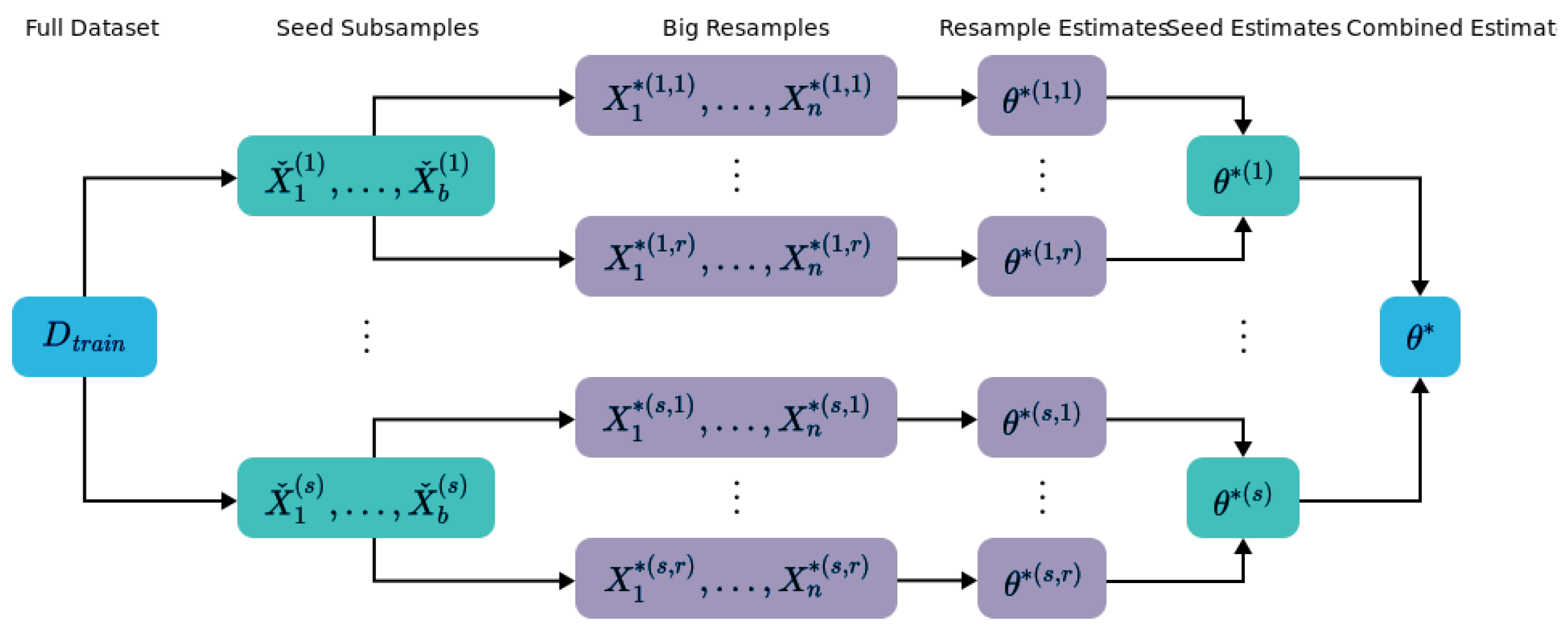
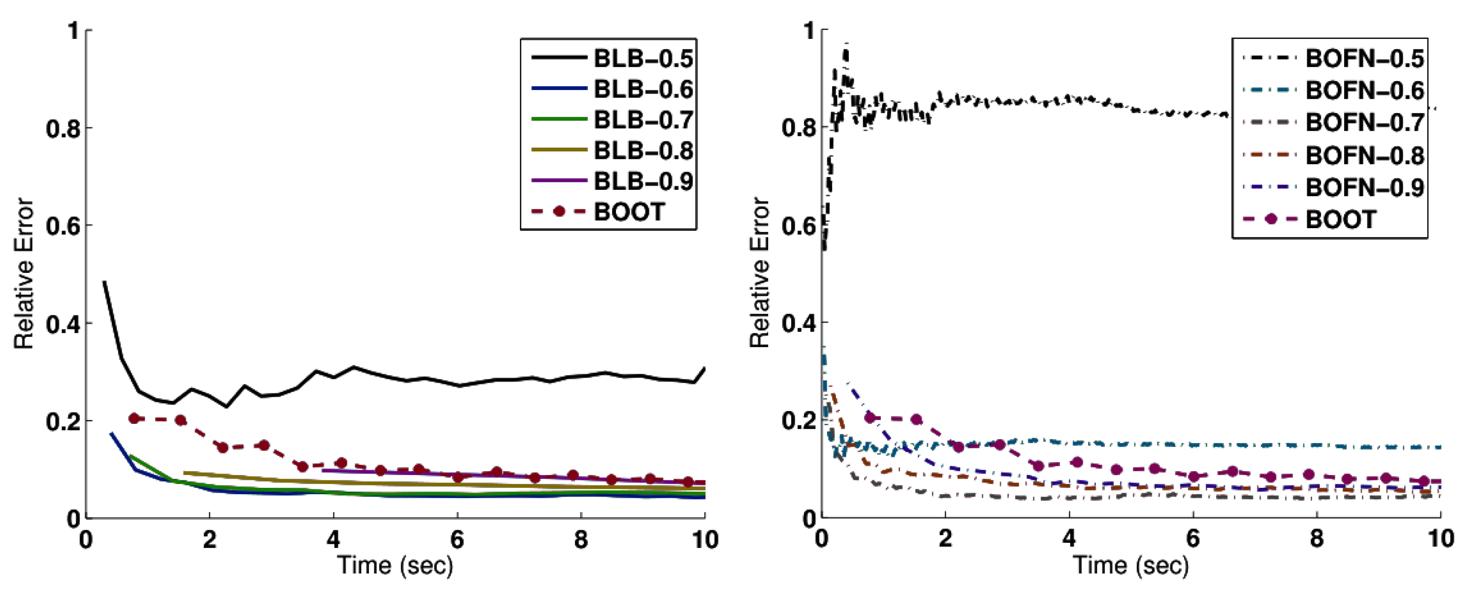
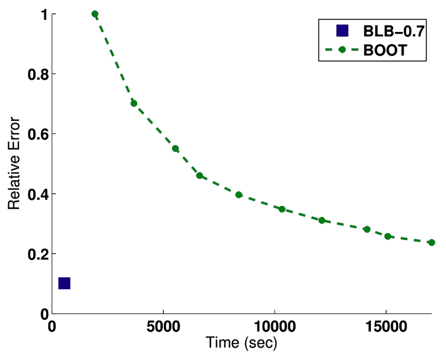
4.1. Bag of Little Bootstraps

The first approach we will discuss is called Bag of Little Bootstraps (BLB) [63,64]. It is a bagging method that combines subsampling with bootstrapping and is particularly well-suited for parallelized implementations.

In the context of Big Data training typically cannot be performed on the entire dataset. A naïve way to solve this problem is to simply train on a random b out of n subsample of the data ${\mathcal{D}}_{\mathit{train}}=\{X_1,\cdots ,X_n\}$. This approach is highly sensitive to noise in the training dataset, especially if $b\ll n$. To overcome this problem bootstrapping can be used. The regular n out of n bootstrapping technique for variance reduction is not suitable for big datasets because it uses $63\%$ of the training data on average. However the b out of n bootstrapping (BOFN) approach can in principle be applied. It uses s samples $\{{\check{X}}^{\left(i\right)}=({\check{X}}_1^{\left(i\right)},\cdots ,{\check{X}}_b^{\left(i\right)})|1\le i\le s\}$ of b datapoints each. Since this approach independently learns s hypotheses $h_i$ on small datasets ${\check{X}}^{\left(i\right)}$, their parameterizations ${\theta }_i$ tend to have large confidence intervals. Because of that, the quality of the combined hypothesis is strongly dependent on b [65]. BLB reduces this dependence.

4.1.1. Intuition

BLB is a simple extension of BOFN that is consistently more robust regarding the choice b across datasets. The basic idea is to add another sampling step. BLB uses each subsample ${\check{X}}^{\left(i\right)}$ as a seed for n out of b sampling. This yields bigger resamples $\{X^{\ast (i,k)}=(X_1^{\ast (i,k)},\cdots ,X_n^{\ast (i,k)})|1\le i\le s,1\le k\le r\}$ that each contain at most b different elements. Training is then run on the resamples $X^{\ast }$ instead of the small seed samples $\check{X}$. The learned hypothesis parameterizations are finally combined into a single hypothesis parameterization ${\theta }^{\ast }$ via a model-specific combination function, e.g., by simply taking the average. Figure 7 (left) shows the first step of BLB, which can reduce variance but it does not guarantee speedup. Figure 7 (right) shows the next step of BLB, where it can speedup training if $\mathcal{O}\left(s{b}^{\alpha }\right)<\mathcal{O}\left(n^{\alpha }\right),\alpha \ge 1$. However, it is sensitive to the choice of b. Lastly, Figure 8 illustrates all steps represented by counts in $\mathcal{O}(blogn)$.

Even though BLB trains classifiers on resamples of size n its time and space complexity effectively still depends on b, not n. This is because each resample $X^{\ast }$ only contains, at most, b different elements which means that it can be efficiently represented by a list of b multiplicity counts $(c_1,\cdots ,c_b)\in {\mathbb{N}}^b$, i.e., $\mathit{space}=\mathcal{O}(blogn)$. Training on such a dataset is equivalent to training on a dataset of size b with weights $w_i=\frac{c_i}{n}$. Since most commonly used classifiers support weighted samples, BLB is widely applicable.

4.1.2. Evaluation

To show the advantages of BLB for classification it was evaluated with logistic regression on a randomly generated dataset. Figure 9 shows that BLB converges on a solution much faster than the regular n out of n bootstrapping (BOOT) with comparable results. It also shows that BLB is less sensitive to the choice of b than BOFN. BLB reached good results with $b\ge n^{0.6}$ whereas BOFN required at least $b\ge n^{0.7}$.

Since training is over proportionally quicker on tiny samples, BLB already outperforms BOOT without parallelism, but it becomes clearer how scalable it is when it is done in parallel. Figure 10 shows that BLB significantly outperforms BOOT on a Spark cluster with 10 workers. This is because each worker node assigned to a BLB sample can store it in memory. Contrarily, the significantly larger BOOT samples need disk reads for large datasets, which accounts for the significant variation in runtime. However, BLB still performs better even if the BOOT samples are cached in RAM since training on the compact BLB samples is over proportionally faster than training on standard bootstrap samples.

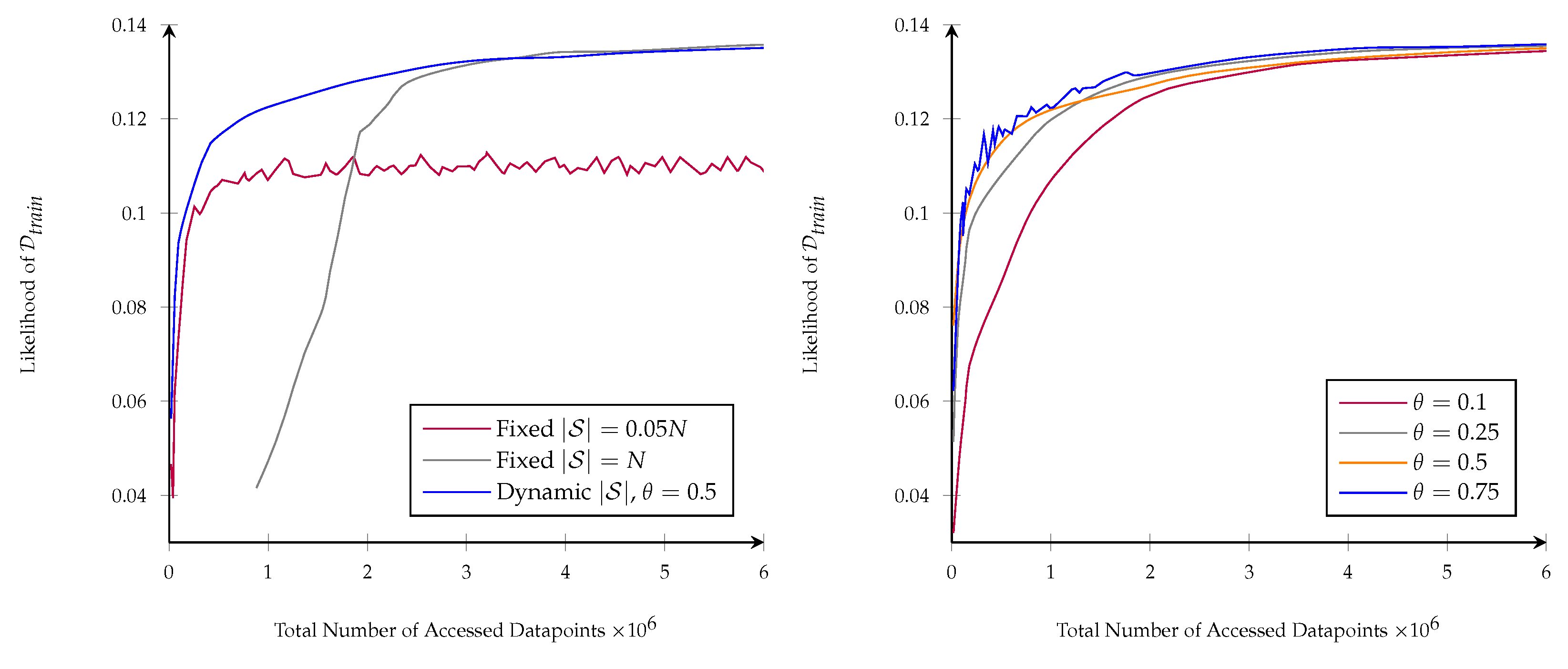
4.2. Subsample Size Selection for Gradient Descent

Next, we will discuss an optimization technique for stochastic gradient descent (SGD). The size of the subsample $\mathcal{S}$ that is considered in a single gradient descent step heavily influences the optimizer’s behavior:

• In the stochastic approximation regime small samples, typically $\left|\mathcal{S}\right|=1$, are used. This causes fast but noisy steps.
• In the batch regime large samples are used, typically $\left|\mathcal{S}\right|=N$ with $N:=|{\mathcal{D}}_{\mathit{train}}|$. Steps are expensive to compute but more reliable.

Typically, neither extreme is appropriate for Big Data applications. The compute clusters that are normally available today are not a good fit for very tiny samples since they cannot be parallelized adequately. The gradients for very big samples however are often too slow to compute. $\left|\mathcal{S}\right|$ should ideally lie somewhere in between.

4.2.1. Size Selection Method

Byrd et al. [66] describe an iterative algorithm that dynamically increases the size of $\mathcal{S}$ as long as this promises to significantly reduce the gradient noise. Let $\mathcal{S}\subseteq \{1,\cdots ,N\}$ describe a random subsample of ${\mathcal{D}}_{\mathit{train}}=\left\{(x_i,y_i)\right|1\le i\le N\}$. SGD will take a step in the descent direction $d=-\nabla J_{\mathcal{S}}\left(w\right)$ where $J_{\mathcal{S}}\left(w\right):=\frac{1}{\left|\mathcal{S}\right|}{\sum }_{i\in \mathcal{S}}\ell (h_w\left(x_i\right),y_i)$ is the differentiable average loss on $\mathcal{S}$ given the current configuration w. Let $J\left(w\right)$ be the average loss on the entire dataset ${\mathcal{D}}_{\mathit{train}}$. $J\left(w\right)$ is the objective function we want to minimize. Our goal is to trade off $\left|\mathcal{S}\right|$ s. t. it is as small as possible while $\nabla J_{\mathcal{S}}\left(w\right)$ still tends to converge with the objective gradient $\nabla J\left(w\right)$, or more formally:

$$\begin{array}{c}\hfill min\left|\mathcal{S}\right|\mathrm{s}.\mathrm{t}.\parallel \nabla J_{\mathcal{S}}{\left(w\right)-\nabla J\left(w\right)\parallel }_2\le \theta {\parallel \nabla J_{\mathcal{S}}\left(w\right)\parallel }_2,\theta \in [0,1)\end{array}$$

(46)

The above equation can also be expressed using a different norm instead of the L2 norm, such as the L1 norm. This can be represented as follows.

$$min\left|\mathcal{S}\right|\mathrm{s}.\mathrm{t}.|\nabla J_{\mathcal{S}}\left(w\right)-\nabla J\left(w\right)|1\le \theta |\nabla J\mathcal{S}\left(w\right)|1,\theta \in [0,1)$$

(47)

Another way is to incorporate a learning rate schedule, where the subsample size is adjusted based on the current learning rate. This can be represented as follows.

$$min\left|\mathcal{S}\right|\mathrm{s}.\mathrm{t}.|\nabla J\mathcal{S}\left(w\right)-\nabla J\left(w\right)|2\le {\theta |\nabla J\mathcal{S}\left(w\right)|}_2,\theta \in [0,1),\mathrm{where}\theta =f\left({\eta }_t\right)$$

(48)

where (f) is a function that maps the current learning rate $\left({\eta }_t\right)$ to a value of $\left(\theta \right)$ and $\left({\eta }_t\right)$ is the learning rate at iteration t.

A value of $\theta =0$ means that $\nabla J_{\mathcal{S}}\left(w\right)$ always has to be equal to $\nabla J\left(w\right)$, whereas $\theta =1$ would allow steps that directy oppose $\nabla J\left(w\right)$. Since it is infeasible to compute $\nabla J\left(w\right)$, condition (46) can however not be checked directly. We will instead resort to an estimate and check whether the condition is satisfied in expectation:

$$\begin{array}{c}\hfill \underset{=\parallel {\mathrm{Var}}_{\mathcal{S}}(\nabla J_{\mathcal{S}}\left(w\right)){\parallel }_1}{\underbrace{{\mathbb{E}}_{\mathcal{S}}[\parallel \nabla J_{\mathcal{S}}\left(w\right)-\nabla J\left(w\right){\parallel }_2^2]}}\le {\theta }^2{\parallel \nabla J_{\mathcal{S}}\left(w\right)\parallel }_2^2\end{array}$$

(49)

Computing ${\mathrm{Var}}_{\mathcal{S}}(\nabla J_{\mathcal{S}}\left(w\right))$ directly is also infeasible because it would require considering all samples of a certain size. Given a sample $\mathcal{S}$, the variance of all samples of that size can instead be approximated by Equation (50).

$$\begin{array}{c}\hfill \parallel {\mathrm{Var}}_{\mathcal{S}}(\nabla J_{\mathcal{S}}\left(w\right)){\parallel }_1\approx \frac{1}{\left|\mathcal{S}\right|\left(\right|\mathcal{S}|-1)}\sum _{i\in \mathcal{S}}{\parallel \nabla \ell (h_w\left(x_i\right),y_i)-\nabla J_{\mathcal{S}}\left(w\right)\parallel }_2^2\end{array}$$

(50)

This approximation assumes that $\left|\mathcal{S}\right|\ll N$. Using (50) we can now estimate (49) which in turn estimates (46). In order to estimate the expectation in the constraint (46), we need to compute the variance of the subsampled gradient.

$$\begin{array}{c}\hfill \mathrm{Var}\mathcal{S}(\nabla J\mathcal{S}\left(w\right))=\frac{1}{\left|\mathcal{S}\right|}\sum _{i\in \mathcal{S}}{(\nabla J_{\mathcal{S}}\left(w\right)-\mathbb{E}[\nabla J_{\mathcal{S}}\left(w\right)])}^2\end{array}$$

(51)

We can now use the above equation to estimate the size of the subsample that we need to use.

$$\left|\mathcal{S}\right|=\frac{|\nabla J_{\mathcal{S}}\left(w\right)|2^2}{\mathrm{Var}\mathcal{S}(\nabla J_{\mathcal{S}}\left(w\right))}\le \frac{{\theta }^2}{1-{\theta }^2}{|\nabla J_{\mathcal{S}}\left(w\right)|}_2^2$$

(52)

If we estimate that (49) is not satisfied for a given $\mathcal{S}$, i.e., that the sample gradient is likely to deviate significantly from the objective gradient, a larger sample $\widehat{\mathcal{S}}$ has to be used. In principle we could simply increase the sample size by a constant amount repeatedly and recheck (49) but this is slow if $\left|\mathcal{S}\right|$ is far off from satisfying the condition. Instead we will adaptively choose $|\widehat{\mathcal{S}}|$ s. t. it is expected to satisfy (49) directly:

$$\begin{array}{c}\hfill |\widehat{\mathcal{S}}|=\frac{\left|\mathcal{S}\right|\parallel {\mathrm{Var}}_{\mathcal{S}}(\nabla J_{\mathcal{S}}\left(w\right)){\parallel }_1}{{\theta }^2{\parallel \nabla J_{\mathcal{S}\left(w\right)}\parallel }_2^2}\end{array}$$

(53)

Please refer to Byrd et al. [66] chapter 3 for a more detailed explanation of (50) and (53). To incorporate the ideas described above into the regular SGD algorithm, (49) has to be checked after each gradient descent step. If the check fails, the size of the following samples has to be increased according to (53). Good values for the initial sample size $|{\mathcal{S}}_0|$ and for $\theta$ have to be found via hyperparameter optimization.

The idea outlined above can similarly also be applied to other gradient-based optimization methods like the curvature-aware Newton Conjugate Gradient (NCG) method. It not only uses $\nabla J_{\mathcal{S}}\left(w\right)$ but also information from the Hessian ${\nabla }^2{J}_{\mathcal{S}}\left(w\right)$ to compute the direction d of the next step. We refer to Byrd et al. [66] chapter 5 for the details.

4.2.2. Evaluation

Subsample size selection was evaluated on a multi-class logistic regression problem using NCG for optimization. At first we look at the accuracy of the estimation of (46) via (50) and (49). On average $\parallel {\mathrm{Var}}_{\mathcal{S}}(\nabla J_{\mathcal{S}}\left(w\right)){\parallel }_1$ deviates about 4% from $\parallel \nabla J_{\mathcal{S}}{\left(w\right)-\nabla J\left(w\right)\parallel }_2$ on the evaluation dataset if $\left|\mathcal{S}\right|\ll N$ [66] tbl.5.1.

Figure 11 shows that this accuracy is sufficient. Dynamic subsample size selection reaches the same quality as the batch method (fixed $\left|\mathcal{S}\right|=N$) while using significantly fewer data points. This in turn makes it significantly faster. The speed of convergence however does depend on the choice of $\theta$. If $\theta$ is too small (see $\theta =0.1$), $\left|\mathcal{S}\right|$ is increased quickly which slows down the optimization. If $\theta$ is too big (see $\theta =0.75$), $\nabla J_{\mathcal{S}}\left(w\right)$ is allowed to deviate significantly from $\nabla J\left(w\right)$ which causes more erratic gradient steps.

4.3. Subsampling for Logistic Regression

We will now look at a method that optimizes the subsample selection process for logistic regression. Subsampling usually increases the mean squared error (MSE) of the resulting hypothesis compared to one that is trained on the full dataset ${\mathcal{D}}_{\mathit{train}}$. Let $\mathcal{S}:=\{{(x_i^{\ast },y_i^{\ast })\}}_{i=1}^r$ be a random subsample of ${\mathcal{D}}_{\mathit{train}}$ that is drawn with or without replacement according to the probabilities ${\left\{{\pi }_i\right\}}_{i=1}^N$ where $N=|{\mathcal{D}}_{\mathit{train}}|$ and ${\sum }_{i=1}^N{\pi }_i=1$. Usually $\mathcal{S}$ is drawn from a uniform distribution, i.e., each datapoint $x_i$ is drawn with probability ${\pi }_i=N^{-1}$. Then a maximum likelihood estimate (MLE) ${\beta }_{\mathcal{S}}=({\beta }_{\mathcal{S}}^{\left(1\right)},\cdots ,{\beta }_{\mathcal{S}}^{\left(d\right)})$ is calculated as an estimate of the objective parameter vector ${\beta }_{{\mathcal{D}}_{\mathit{train}}}$ that maximizes the likelihood of the entire dataset. This strategy is often not optimal since some data points might have a smaller influence on ${\beta }_{{\mathcal{D}}_{\mathit{train}}}$ than others. The core idea now is to choose the probabilities ${\pi }_i$ s. t. more informative data points are more likely to be sampled.

4.3.1. Case Control

A simple idea to adjust the sampling probabilities ${\pi }_i$ is to use Case-Control subsampling (CC) in which a roughly equal amount of positive and negative samples is drawn. Let ${\mathcal{D}}_{\mathit{train}}^{+}:=\{(x,y)\in {\mathcal{D}}_{\mathit{train}}|y=1\}$ and ${\mathcal{D}}_{\mathit{train}}^{-}:=\{(x,y)\in {\mathcal{D}}_{\mathit{train}}|y=0\}$. CC samples would be then chosen without replacement with probabilities

$$\begin{array}{c}\hfill {\pi }_i=\left\{\begin{array}{cc}|{\mathcal{D}}_{\mathit{train}}^{+}{|}^{-1}\hfill & \mathrm{if}{y}_i=1\hfill \\ |{\mathcal{D}}_{\mathit{train}}^{-}{|}^{-1}\hfill & \mathrm{if}{y}_i=0\hfill \end{array}\right.\end{array}$$

(54)

4.3.2. Local Case Control

Fithian and Hastie [67] proposed Local Case-Control subsampling (LCC) to remove the bias from CC. LCC determines the sampling probabilities ${\pi }_i$ via a pilot estimate ${\beta }_0$. The estimate ${\beta }_0$ is the MLE of a small pilot sample ${\mathcal{S}}_0$ that is drawn with uniform or CC sample probabilities. CC sampling should only be used for the pilot if ${\mathcal{D}}_{\mathit{train}}$ contains an imbalanced amount of positive and negative samples. After determining the pilot estimate ${\beta }_0$, datapoints are weighted by the error of the pilot estimator on them:

$$\begin{array}{c}\hfill {\pi }_i=\frac{|y_i-p\left(x_i\right|{\beta }_0)|}{{\sum }_{j=1}^N|y_j-p\left(x_j\right|{\beta }_0)|}\mathrm{with}p\left(x\right|\beta )=\frac{1}{1+exp\left({\beta }^{T}x\right)}\end{array}$$

(55)

Then a greater sample ${\mathcal{S}}_{\mathrm{LCC}}$ is drawn using those probabilities, typically with replacement since this is computationally less expensive. This produces an estimate ${\beta }_{{\mathcal{S}}_{\mathrm{LCC}}}$ that is consistent with ${\beta }_{{\mathcal{D}}_{\mathit{train}}}$, i.e., $\parallel {\beta }_{{\mathcal{S}}_{\mathrm{LCC}}}-{\beta }_{{\mathcal{D}}_{\mathit{train}}}{\parallel }_2\to 0$ as $r\to \infty$. Additionally, LCC prioritizes data points that are close to the decision boundary estimated by the pilot. This tends to reduce the variance of the estimate ${\beta }_{{\mathcal{S}}_{\mathrm{LCC}}}$, especially if ${\mathcal{D}}_{\mathit{train}}$ contains an imbalanced amount of positive and negative samples.

4.3.3. OSMAC

While LCC tends to reduce the estimate’s variance, it does not necessarily minimize it. The Optimal Subsampling Motivated by the A-Optimality Criterion (OSMAC) [68,69] method improves upon LCC by minimizing the expected variance. Like LCC it also uses a pilot estimate ${\beta }_0$ but the sampling probabilities ${\pi }_i$ are then calculated differently.

Let $V:=\mathrm{Cov}({\beta }_{\mathcal{S}}-{\beta }_{{\mathcal{D}}_{\mathit{train}}})$ be the covariance matrix of the difference between the sample estimate and the complete dataset estimate. Given $\mathbb{E}[{\beta }_{\mathcal{S}}-{\beta }_{{\mathcal{D}}_{\mathit{train}}}]=0$, V can be interpreted as a measure of the expected error introduced by subsampling. Using the A-optimality criterion of optimal design, OSMAC sets the sampling probabilities ${\pi }_i$ so that $\mathrm{tr}\left(V\right)$ is minimized in expectation. More intuitively this minimizes the sum of the MSEs on the regression coefficients ${\beta }_{\mathcal{S}}^{\left(k\right)}$, i.e., ${\sum }_{k=1}^d\mathbb{E}\left[{({\beta }_{\mathcal{S}}^{\left(k\right)}-{\beta }_{{\mathcal{D}}_{\mathit{train}}}^{\left(k\right)})}^2\right]$.

It turns out that finding the minimizing probabilities ${\pi }_i$ of $\mathrm{tr}\left(V\right)$ is computationally expensive. However the optimal values for ${\pi }_i$ can be approximated using

$$\begin{array}{c}\hfill {\pi }_i=\frac{|y_i-p\left(x_i\right|{\beta }_0)|·\parallel x_i{\parallel }_2}{{\sum }_{j=1}^N|y_j-p\left(x_j\right|{\beta }_0)|·\parallel x_j{\parallel }_2}\end{array}$$

(56)

The main difference to LCC here is the added $\parallel x_i{\parallel }_2$ factor. The intuition behind this is that samples with large norms tend to be further away from the decision boundary (this intuition is not entirely correct since it does not consider the offset and rotation of the decision boundary. Those aspects are ignored because (56) only approximates the A-optimal probabilities). An incorrectly classified sample that is far from the decision boundary is more surprising than an incorrectly classified sample close to it. Since the sigmoidal p function saturates quickly this fact is often not captured by LCC sampling.

4.3.4. Evaluation

We will now compare uniform, LCC, and OSMAC sampling on two datasets. The data points $x_i$ are randomly sampled from different distributions. The corresponding classes $y_i\in \{0,1\}$ are then assigned using a fixed coefficient vector $\beta$. These two datasets are used:

• mzNormal: Uses a multivariate normal distribution $\mathcal{N}(0,\Sigma )$ with mean 0 and ${\Sigma }_{ij}=0.5^{{\delta }_{i\ne j}}$. Contains a roughly equal amount of positive and negative samples.
• nzNormal: Uses a multivariate normal distribution $\mathcal{N}(1.5,\Sigma )$ with mean $1.5$. About 95% of the samples are positive.

Figure 12 shows the MSEs $\parallel {\beta }_{\mathcal{S}}{-\beta \parallel }_2^2$ for different subsample sizes r. OSMAC consistently gives the closest approximation of $\beta$, confirming its theoretical A-optimality. The reduced coefficient approximation error in turn results in a reduced error of OSMAC on ${\mathcal{D}}_{\mathit{train}}$.

4.4. Clustering for SVMs

To speed up the training of SVMs De Almeida et al. [70] proposed a simple method that reduces the dataset size via k-means clustering. It can be described as a simple three-step procedure:

• Group the training samples ${\mathcal{D}}_{\mathit{train}}$ into k clusters $C_1,\cdots ,C_k$ with centers $c_1,\cdots ,c_k$ where k should be determined via hyperparameter optimization.
• Check for each cluster $C_i$ whether all associated data points belong to the same class, i.e., $\exists z\in \{+1,-1\}:\forall (x,y)\in C_i:y=z$. If yes, all datapoints in $C_i$ are removed from ${\mathcal{D}}_{\mathit{train}}$ and replaced by $c_i$. If not, they are kept in the dataset. The intuition behind this is that clusters with points from multiple classes might be near the decision boundary so they are kept to serve as potential support vectors.
• Finally standard SVM training is performed on the reduced training dataset.

The effectiveness of this method is comparable to SVM training on the entire dataset. The decreased dataset size, however, is incredibly variable. We won’t attempt to minimize the dataset size by using large homogenous clusters with just a few noisy outliers belonging to a different class. Because of this, depending on the dataset, the effective speedup and memory requirements may vary substantially.

Lee et al. [71] proposed KM-SVM, an alternative approach that solves this problem by performing clustering on the data points of each class separately. This method has more predictable time and memory requirements, but it also tends to modify the structure of the dataset. WKM-SVM [72] improves upon KM-SVM by weighting each cluster center $c_i$ by the amount of datapoints $|C_i|$ it represents. This solves the problem that small clusters of outliers have the same influence on the decision boundary as big clusters of more representative data points in KM-SVM.

4.4.1. Evaluation

We will now compare KM-SVM and WKM-SVM using different compression rates $R\in \{1,3,5,10\}$ that describe the number of clusters $k=\frac{|{\mathcal{D}}_{\mathit{train}}|}{R}$. A compression rate of $R=1$ corresponds to an SVM that is trained on the entire dataset. For ${\mathcal{D}}_{\mathit{train}}$ the PimaIndiansDiabetes2 dataset is used. Figure 13 shows that WKM-SVM consistently performs better than KM-SVM with a roughly identical training time. Both clustering methods improve the runtime significantly without any significant increases in the test error.

5. Discussion

The field of automated machine learning (AutoML) has gained significant attention due to its potential to automate the process of building and optimizing machine learning models. As the amount of big data being generated continues to grow, new challenges for AutoML systems arise in terms of big data management. This paper introduces a comprehensive framework that combines multiple techniques for hyperparameter optimization and training acceleration, which are essential components in AutoML systems.

Our proposed framework distinguishes itself from existing literature by integrating various techniques, such as Fabolas and learning curve extrapolation for hyperparameter optimization, and Bag of Little Bootstraps, k-means clustering for Support Vector Machines, subsample size selection for gradient descent, and subsampling for logistic regression for training acceleration. This multi-faceted approach allows for a more efficient and adaptable training process that can be tailored to different learning scenarios.

The contributions of our paper are twofold. First, we provide an in-depth investigation of Fabolas and learning curve extrapolation as methods for accelerating hyperparameter optimization, reducing the computational costs associated with hyperparameter tuning. Second, we explore four training acceleration techniques and demonstrate how they can be combined with the hyperparameter optimization methods for even greater speedups in training. Feature selection and dimensionality reduction are important AutoML techniques that warrant further exploration. While our framework focuses on hyperparameter optimization and training acceleration, future work could investigate adaptive selection and weighting of features for dimensionality reduction and performance improvement, as suggested by the recent literature [73,74,75].

In conclusion, this paper contributes to the field by proposing a comprehensive and adaptable framework for accelerating training on large datasets. We have demonstrated the effectiveness of combining hyperparameter optimization and training optimization techniques and acknowledge the potential for further exploration in feature selection and dimensionality reduction. By leveraging these advanced techniques, practitioners and researchers can effectively tackle the challenges of training complex models on large datasets, ultimately contributing to the development of more powerful and efficient machine-learning solutions in the AutoML domain.

6. Conclusions and Future Work

In this article, we investigated Fabolas and learning curve extrapolation as two methods for accelerating hyperparameter optimization. Both employ probabilistic models to gauge the error values of the function. The following four methods for accelerating training were then presented: Bag of Little Bootstraps, k-means clustering for SVMs, subsample size selection for gradient descent, and subsampling for logistic regression. All of the methodologies discussed can greatly speed up training on large datasets. These methods enhance various facets of the training process, making it feasible to combine them in diverse ways to gain further speedups.

We reviewed several combinations that have potential: Fabolas may be easily coupled with any of the training optimization strategies described in Section 4 since it is a hyperparameter optimizer that does not make learner assumptions. The learner utilizing gradient descent is necessary for the learning curve extrapolation approach mentioned in Section 3.3. Thus, it may be used in conjunction with the technique for choosing the subsample size given in Section 4.2. Fabolas and learning curve extrapolation might also be used together to direct the hyperparameter search, however, in order to do this, the covariance kernel of the cost model c would need to be changed. This is because samples placed in less desirable locations are more likely to be terminated early, which reduces their cost and increases their attractiveness to the acquisition function $a_F$. Including a dependency on the loss model f is one way to modify the cost model. This would essentially merge the two Gaussian processes c and f into a single cost-loss model over the parameter space $\Theta =\Lambda \times [0,1]\times \{\mathrm{cost},\mathrm{loss}\}$ where information about the loss of a configuration is indicative about its cost. Finding a suitable kernel function for this joint GP model could be a subject of further research.

Since it is a general-purpose bagging technique, Bag of Little Bootstraps (Section 4.1) may theoretically be coupled with the other three training optimization techniques. The latter, however, relies on dynamically adjusting the sample size during training in order to lower the anticipated variance, making the coupling of BLB with subsample size selection for gradient descent difficult. This approach does not work well if the training data is a resampled BLB bootstrap that does not allow for significant variance reduction since it only contains a small fraction of data points. The combinations of BLB with OSMAC and BLB with WKM-SVM are more promising. In the case of OSMAC the sampling weights $\left({\pi }_i\right)$ could be used to sample the small bootstraps $\check{X}$. Subsample size optimization (Section 4.2) and OSMAC (Section 4.3) are two more potential combinations. Since gradient descent is frequently used to execute logistic regression, both approaches can be coupled by utilizing OSMAC to obtain the subsample for each SGD step.

In addition to these combinations, several other possible approaches can be used to further speed up training on large datasets. One such approach is to utilize distributed computing frameworks such as Apache Spark or Apache Kafka. These frameworks allow for the parallel processing of large datasets, which can greatly speed up the training process. Another possible future direction is to utilize MCMC (Markov Chain Monte Carlo) methods or Hamiltonian Monte Carlo (HMC) for hyperparameter optimization. These methods can be used to efficiently explore the parameter space, and have been shown to be effective in a variety of applications. Additionally, Using Hidden Markov Models (HMM) is a possible approach, as they are particularly well suited for sequential data such as time series, signals, speech, and image data. They can be used to model the underlying structure of the data, which can be useful in training models with large datasets. Furthermore, they can also be used to implement online learning, which allows for models to be updated in real-time as new data is acquired.

In summary, the proposed techniques presented in this paper have significant practical implications for processing large datasets and efficient large-scale training. The use of probabilistic models for hyperparameter optimization, such as Fabolas and learning curve extrapolation, can be combined with techniques like Bag of Little Bootstraps, k-means clustering for SVMs, subsample size selection for gradient descent, and subsampling for logistic regression for even greater speedups. Additionally, distributed computing frameworks, MCMC methods, HMC, and HMM are possible future directions for further speedup. Future research may focus on evaluating these combinations of various techniques and exploring the potential of these other approaches to accelerate the training process on large datasets and future research should explore additional methods for speedup.

References

1. Kang, J.S.; Kang, J.; Kim, J.J.; Jeon, K.W.; Chung, H.J.; Park, B.H. Neural Architecture Search Survey: A Computer Vision Perspective. Sensors 2023, 23, 1713. [Google Scholar] [CrossRef]
2. Baymurzina, D.; Golikov, E.; Burtsev, M. A review of neural architecture search. Neurocomputing 2022, 474, 82–93. [Google Scholar] [CrossRef]
3. Lindauer, M.; Hutter, F. Best Practices for Scientific Research on Neural Architecture Search. J. Mach. Learn. Res. 2020, 21, 9820–9837. [Google Scholar]
4. Jin, H.; Song, Q.; Hu, X. Auto-Keras: An Efficient Neural Architecture Search System. In Proceedings of the 25th ACM SIGKDD International Conference on Knowledge Discovery & Data Mining (KDD ’19), Anchorage, AK, USA, 4–8 August 2019; Association for Computing Machinery: New York, NY, USA, 2019; pp. 1946–1956. [Google Scholar] [CrossRef] [Green Version]
5. Figueiredo, E.; Park, G.; Farrar, C.R.; Worden, K.; Figueiras, J. Machine learning algorithms for damage detection under operational and environmental variability. Struct. Health Monit. 2011, 10, 559–572. [Google Scholar] [CrossRef]
6. Susto, G.A.; Schirru, A.; Pampuri, S.; McLoone, S.; Beghi, A. Machine learning for predictive maintenance: A multiple classifier approach. IEEE Trans. Ind. Inform. 2014, 11, 812–820. [Google Scholar] [CrossRef] [Green Version]
7. Li, H.; Parikh, D.; He, Q.; Qian, B.; Li, Z.; Fang, D.; Hampapur, A. Improving rail network velocity: A machine learning approach to predictive maintenance. Transp. Res. Part Emerg. Technol. 2014, 45, 17–26. [Google Scholar] [CrossRef]
8. Stühler, E.; Braune, S.; Lionetto, F.; Heer, Y.; Jules, E.; Westermann, C.; Bergmann, A.; van Hövell, P. Framework for personalized prediction of treatment response in relapsing remitting multiple sclerosis. BMC Med. Res. Methodol. 2020, 20, 24. [Google Scholar] [CrossRef] [Green Version]
9. Handzic, M.; Tjandrawibawa, F.; Yeo, J. How neural networks can help loan officers to make better informed application decisions. Informing Sci. 2003, 6, 97–109. [Google Scholar]
10. Viaene, S.; Dedene, G.; Derrig, R.A. Auto claim fraud detection using Bayesian learning neural networks. Expert Syst. Appl. 2005, 29, 653–666. [Google Scholar] [CrossRef]
11. Pérez, J.M.; Muguerza, J.; Arbelaitz, O.; Gurrutxaga, I.; Martín, J.I. Consolidated tree classifier learning in a car insurance fraud detection domain with class imbalance. In Proceedings of the International Conference on Pattern Recognition and Image Analysis, Bath, UK, 23–25 August 2005; Springer: Berlin/Heidelberg, Germany, 2005; pp. 381–389. [Google Scholar]
12. Tsoumakas, G. A survey of machine learning techniques for food sales prediction. Artif. Intell. Rev. 2019, 52, 441–447. [Google Scholar] [CrossRef]
13. Karras, C.; Karras, A.; Tsolis, D.; Avlonitis, M.; Sioutas, S. A Hybrid Ensemble Deep Learning Approach for Emotion Classification. In Proceedings of the 2022 IEEE International Conference on Big Data (Big Data), Atlanta, GA, USA, 17–20 December 2022; pp. 3881–3890. [Google Scholar] [CrossRef]
14. Li, L.; Jamieson, K.; DeSalvo, G.; Rostamizadeh, A.; Talwalkar, A. Hyperband: A novel bandit-based approach to hyperparameter optimization. J. Mach. Learn. Res. 2017, 18, 6765–6816. [Google Scholar]
15. Duan, J.; Zeng, Z.; Oprea, A.; Vasudevan, S. Automated generation and selection of interpretable features for enterprise security. In Proceedings of the 2018 IEEE International Conference on Big Data (Big Data), Seattle, WA, USA, 10–13 December 2018; pp. 1258–1265. [Google Scholar]
16. Andrychowicz, M.; Denil, M.; Gómez, S.; Hoffman, M.W.; Pfau, D.; Schaul, T.; Shillingford, B.; de Freitas, N. Learning to learn by gradient descent by gradient descent. In Advances in Neural Information Processing Systems; Lee, D., Sugiyama, M., Luxburg, U., Guyon, I., Garnett, R., Eds.; Curran Associates, Inc.: New York, NY, USA, 2016; Volume 29. [Google Scholar]
17. Zoph, B.; Le, Q.V. Neural architecture search with reinforcement learning. arXiv 2016, arXiv:1611.01578. [Google Scholar]
18. Feurer, M.; Klein, A.; Eggensperger, K.; Springenberg, J.; Blum, M.; Hutter, F. Efficient and robust automated machine learning. Adv. Neural Inf. Process. Syst. 2015, 28. [Google Scholar]
19. Gaudel, R.; Sebag, M. Feature selection as a one-player game. In Proceedings of the International Conference on Machine Learning, Haifa, Israel, 21–25 June 2010; pp. 359–366. [Google Scholar]
20. Katz, G.; Shin, E.C.R.; Song, D. Explorekit: Automatic feature generation and selection. In Proceedings of the 2016 IEEE 16th International Conference on Data Mining (ICDM), Barcelona, Spain, 12–15 December 2016; pp. 979–984. [Google Scholar]
21. Nargesian, F.; Samulowitz, H.; Khurana, U.; Khalil, E.B.; Turaga, D.S. Learning Feature Engineering for Classification. In Proceedings of the IJCAI, Melbourne, Australia, 19–25 August 2017; pp. 2529–2535. [Google Scholar]
22. Kaul, A.; Maheshwary, S.; Pudi, V. Autolearn—Automated feature generation and selection. In Proceedings of the 2017 IEEE International Conference on data mining (ICDM), New Orleans, LA, USA, 18–21 November 2017; pp. 217–226. [Google Scholar]
23. Meinshausen, N.; Bühlmann, P. Stability selection. J. R. Stat. Soc. Ser. (Stat. Methodol.) 2010, 72, 417–473. [Google Scholar] [CrossRef]
24. Pfahringer, B.; Bensusan, H.; Giraud-Carrier, C.G. Meta-Learning by Landmarking Various Learning Algorithms. In Proceedings of the ICML, Stanford, CA, USA, 29 June–2 July 2000; pp. 743–750. [Google Scholar]
25. Klein, A.; Falkner, S.; Springenberg, J.T.; Hutter, F. Learning Curve Prediction with Bayesian Neural Networks. In Proceedings of the ICLR, Toulon, France, 24–26 April 2017. [Google Scholar]
26. Eggensperger, K.; Lindauer, M.; Hutter, F. Neural networks for predicting algorithm runtime distributions. arXiv 2017, arXiv:1709.07615. [Google Scholar]
27. Brazdil, P.B.; Soares, C. A comparison of ranking methods for classification algorithm selection. In Proceedings of the European Conference on Machine Learning, Barcelona, Spain, 31 May–2 June 2000; Springer: Berlin/Heidelberg, Germany, 2000; pp. 63–75. [Google Scholar]
28. Andrychowicz, M.; Denil, M.; Gomez, S.; Hoffman, M.W.; Pfau, D.; Schaul, T.; Shillingford, B.; De Freitas, N. Learning to learn by gradient descent by gradient descent. In Proceedings of the 30th International Conference on Neural Information Processing Systems, Barcelona, Spain, 5–10 December 2016. [Google Scholar]
29. Hochreiter, S.; Schmidhuber, J. Long short-term memory. Neural Comput. 1997, 9, 1735–1780. [Google Scholar] [CrossRef]
30. Graves, A. Long short-term memory. In Supervised Sequence Labelling with Recurrent Neural Networks; Springer: Berlin/Heidelberg, Germany, 2012; pp. 37–45. [Google Scholar]
31. Chen, Y.; Hoffman, M.W.; Colmenarejo, S.G.; Denil, M.; Lillicrap, T.P.; Botvinick, M.; Freitas, N. Learning to learn without gradient descent by gradient descent. In Proceedings of the International Conference on Machine Learning, PMLR, Sydney, Australia, 6–11 August 2017; pp. 748–756. [Google Scholar]
32. Cortes, C.; Vapnik, V. Support-vector networks. Mach. Learn. 1995, 20, 273–297. [Google Scholar] [CrossRef]
33. Elsken, T.; Metzen, J.H.; Hutter, F. Simple and efficient architecture search for convolutional neural networks. arXiv 2017, arXiv:1711.04528. [Google Scholar]
34. Real, E.; Moore, S.; Selle, A.; Saxena, S.; Suematsu, Y.L.; Tan, J.; Le, Q.V.; Kurakin, A. Large-scale evolution of image classifiers. In Proceedings of the International Conference on Machine Learning, PMLR, Sydney, Australia, 6–11 August 2017; pp. 2902–2911. [Google Scholar]
35. He, Y.; Lin, J.; Liu, Z.; Wang, H.; Li, L.J.; Han, S. Amc: Automl for model compression and acceleration on mobile devices. In Proceedings of the European Conference on Computer Vision (ECCV), Munich, Germany, 8–14 September 2018; pp. 784–800. [Google Scholar]
36. Guyon, I.; Sun-Hosoya, L.; Boullé, M.; Escalante, H.J.; Escalera, S.; Liu, Z.; Jajetic, D.; Ray, B.; Saeed, M.; Sebag, M.; et al. Analysis of the automl challenge series. Autom. Mach. Learn. 2019, 177–219. [Google Scholar] [CrossRef] [Green Version]
37. Brochu, E.; Cora, V.M.; De Freitas, N. A tutorial on Bayesian optimization of expensive cost functions, with application to active user modeling and hierarchical reinforcement learning. arXiv 2010, arXiv:1012.2599. [Google Scholar]
38. Hutter, F.; Hoos, H.H.; Leyton-Brown, K. Sequential model-based optimization for general algorithm configuration. In Proceedings of the International Conference on Learning and Intelligent Optimization, Rome, Italy, 17–21 January 2011; Springer: Berlin/Heidelberg, Germany, 2011; pp. 507–523. [Google Scholar]
39. Feurer, M.; Springenberg, J.; Hutter, F. Initializing Bayesian Hyperparameter Optimization via Meta-Learning. In Proceedings of the AAAI Conference on Artificial Intelligence, Austin, TX, USA, 25–30 January 2015; Volume 29. [Google Scholar] [CrossRef]
40. Jamieson, K.; Talwalkar, A. Non-stochastic best arm identification and hyperparameter optimization. In Proceedings of the Artificial Intelligence and Statistics, PMLR, Cadiz, Spain, 9–11 May 2016; pp. 240–248. [Google Scholar]
41. Jaderberg, M.; Dalibard, V.; Osindero, S.; Czarnecki, W.M.; Donahue, J.; Razavi, A.; Vinyals, O.; Green, T.; Dunning, I.; Simonyan, K.; et al. Population based training of neural networks. arXiv 2017, arXiv:1711.09846. [Google Scholar]
42. Maclaurin, D.; Duvenaud, D.; Adams, R. Gradient-based hyperparameter optimization through reversible learning. In Proceedings of the International Conference on Machine Learning, PMLR, Lille, France, 6–11 July 2015; pp. 2113–2122. [Google Scholar]
43. Zacharia, A.; Zacharia, D.; Karras, A.; Karras, C.; Giannoukou, I.; Giotopoulos, K.C.; Sioutas, S. An Intelligent Microprocessor Integrating TinyML in Smart Hotels for Rapid Accident Prevention. In Proceedings of the 2022 7th South-East Europe Design Automation, Computer Engineering, Computer Networks and Social Media Conference (SEEDA-CECNSM), Ioannina, Greece, 23–25 September 2022; pp. 1–7. [Google Scholar] [CrossRef]
44. Schizas, N.; Karras, A.; Karras, C.; Sioutas, S. TinyML for Ultra-Low Power AI and Large Scale IoT Deployments: A Systematic Review. Future Internet 2022, 14, 363. [Google Scholar] [CrossRef]
45. Nagarajah, T.; Poravi, G. A Review on Automated Machine Learning (AutoML) Systems. In Proceedings of the 2019 IEEE 5th International Conference for Convergence in Technology (I2CT), Bombay, India, 29–31 March 2019; pp. 1–6. [Google Scholar] [CrossRef]
46. Bahri, M.; Salutari, F.; Putina, A.; Sozio, M. Automl: State of the art with a focus on anomaly detection, challenges, and research directions. Int. J. Data Sci. Anal. 2022, 14, 113–126. [Google Scholar] [CrossRef]
47. Remeseiro, B.; Bolon-Canedo, V. A review of feature selection methods in medical applications. Comput. Biol. Med. 2019, 112, 103375. [Google Scholar] [CrossRef] [PubMed]
48. Isabona, J.; Imoize, A.L.; Kim, Y. Machine Learning-Based Boosted Regression Ensemble Combined with Hyperparameter Tuning for Optimal Adaptive Learning. Sensors 2022, 22, 3776. [Google Scholar] [CrossRef]
49. Guo, P.; Yang, D.; Hatamizadeh, A.; Xu, A.; Xu, Z.; Li, W.; Zhao, C.; Xu, D.; Harmon, S.; Turkbey, E.; et al. Auto-FedRL: Federated Hyperparameter Optimization for Multi-institutional Medical Image Segmentation. In Proceedings of the Computer Vision—ECCV 2022, Tel Aviv, Israel, 23–27 October 2022; Avidan, S., Brostow, G., Cissé, M., Farinella, G.M., Hassner, T., Eds.; Springer Nature Switzerland: Cham, Switzerland, 2022; pp. 437–455. [Google Scholar]
50. Li, Y.; Shen, Y.; Jiang, H.; Zhang, W.; Li, J.; Liu, J.; Zhang, C.; Cui, B. Hyper-Tune: Towards Efficient Hyper-parameter Tuning at Scale. arXiv 2022, arXiv:2201.06834. [Google Scholar] [CrossRef]
51. Passos, D.; Mishra, P. A tutorial on automatic hyperparameter tuning of deep spectral modelling for regression and classification tasks. Chemom. Intell. Lab. Syst. 2022, 223, 104520. [Google Scholar] [CrossRef]
52. Yu, T.; Zhu, H. Hyper-parameter optimization: A review of algorithms and applications. arXiv 2020, arXiv:2003.05689. [Google Scholar]
53. Bischl, B.; Binder, M.; Lang, M.; Pielok, T.; Richter, J.; Coors, S.; Thomas, J.; Ullmann, T.; Becker, M.; Boulesteix, A.L.; et al. Hyperparameter optimization: Foundations, algorithms, best practices, and open challenges. Wiley Interdiscip. Rev. Data Min. Knowl. Discov. 2021, 13, e1484. [Google Scholar] [CrossRef]
54. Sipper, M. High Per Parameter: A Large-Scale Study of Hyperparameter Tuning for Machine Learning Algorithms. Algorithms 2022, 15, 315. [Google Scholar] [CrossRef]
55. Giotopoulos, K.C.; Michalopoulos, D.; Karras, A.; Karras, C.; Sioutas, S. Modelling and Analysis of Neuro Fuzzy Employee Ranking System in the Public Sector. Algorithms 2023, 16, 151. [Google Scholar] [CrossRef]
56. Klein, A.; Falkner, S.; Bartels, S.; Hennig, P.; Hutter, F. Fast Bayesian Optimization of Machine Learning Hyperparameters on Large Datasets. In Proceedings of the 20th International Conference on Artificial Intelligence and Statistics, Ft. Lauderdale, FL, USA, 20–22 April 2017; Singh, A., Zhu, J., Eds.; PMLR: Fort Lauderdale, FL, USA, 2017; Volume 54, pp. 528–536. [Google Scholar]
57. Schön, S.; Kermarrec, G.; Kargoll, B.; Neumann, I.; Kosheleva, O.; Kreinovich, V. Why Student Distributions? Why Matern’s Covariance Model? A Symmetry-Based Explanation. In Econometrics for Financial Applications; Springer International Publishing: Berlin/Heidelberg, Germany, 2017; pp. 266–275. [Google Scholar] [CrossRef] [Green Version]
58. Karras, C.; Karras, A.; Avlonitis, M.; Sioutas, S. An Overview of MCMC Methods: From Theory to Applications. In Proceedings of the Artificial Intelligence Applications and Innovations. AIAI 2022 IFIP WG 12.5 International Workshops, Crete, Greece, 17–20 June 2022; Maglogiannis, I., Iliadis, L., Macintyre, J., Cortez, P., Eds.; Springer International Publishing: Cham, Switzerland, 2022; pp. 319–332. [Google Scholar]
59. Karras, C.; Karras, A.; Tsolis, D.; Giotopoulos, K.C.; Sioutas, S. Distributed Gibbs Sampling and LDA Modelling for Large Scale Big Data Management on PySpark. In Proceedings of the 2022 7th South-East Europe Design Automation, Computer Engineering, Computer Networks and Social Media Conference (SEEDA-CECNSM), Ioannina, Greece, 23–25 September 2022; pp. 1–8. [Google Scholar] [CrossRef]
60. Karras, C.; Karras, A.; Avlonitis, M.; Giannoukou, I.; Sioutas, S. Maximum Likelihood Estimators on MCMC Sampling Algorithms for Decision Making. In Proceedings of the Artificial Intelligence Applications and Innovations. AIAI 2022 IFIP WG 12.5 International Workshops, Crete, Greece, 17–20 June 2022; Maglogiannis, I., Iliadis, L., Macintyre, J., Cortez, P., Eds.; Springer International Publishing: Cham, Switzerland, 2022; pp. 345–356. [Google Scholar]
61. Swersky, K.; Snoek, J.; Adams, R.P. Multi-task Bayesian Optimization. In Advances in Neural Information Processing Systems; NIPS’13; Curran Associates Inc.: New York, NY, USA, 2013; pp. 2004–2012. [Google Scholar]
62. Domhan, T.; Springenberg, J.T.; Hutter, F. Speeding Up Automatic Hyperparameter Optimization of Deep Neural Networks by Extrapolation of Learning Curves. In Proceedings of the 24th International Conference on Artificial Intelligence, Buenos Aires, Argentina, 25–31 July 2015; pp. 3460–3468. [Google Scholar]
63. Kleiner, A.; Talwalkar, A.; Sarkar, P.; Jordan, M.I. A Scalable Bootstrap for Massive Data. J. R. Stat. Soc. Ser. (Stat. Methodol.) 2014, 76, 795–816. [Google Scholar] [CrossRef] [Green Version]
64. Norazan, M.; Habshah, M.; Imon, A.; Chen, S. Weighted bootstrap with probability in regression. In WSEAS International Conference. Proceedings. Mathematics and Computers in Science and Engineering; World Scientific and Engineering Academy and Society: South Wales, Australia, 2009; Volume 8, p. 16. [Google Scholar]
65. Bickel, P.J.; Götze, F.; van Zwet, W.R. Resampling fewer than n observations: Gains, losses, and remedies for losses. Stat. Sin. 1997, 7, 1–31. [Google Scholar]
66. Byrd, R.H.; Chin, G.M.; Nocedal, J.; Wu, Y. Sample size selection in optimization methods for machine learning. Math. Program. 2012, 134, 127–155. [Google Scholar] [CrossRef]
67. Fithian, W.; Hastie, T. Local case-control sampling: Efficient subsampling in imbalanced data sets. Ann. Stat. 2014, 42, 1693. [Google Scholar] [CrossRef] [PubMed] [Green Version]
68. Wang, H. More efficient estimation for logistic regression with optimal subsamples. J. Mach. Learn. Res. 2019, 20, 1–59. [Google Scholar]
69. Wang, H.; Zhu, R.; Ma, P. Optimal Subsampling for Large Sample Logistic Regression. J. Am. Stat. Assoc. 2018, 113, 829–844. [Google Scholar] [CrossRef] [PubMed]
70. De Almeida, M.B.; de Pádua Braga, A.; Braga, J.P. SVM-KM: Speeding SVMs learning with a priori cluster selection and k-means. In Proceedings of the Vol. 1. Sixth Brazilian Symposium on Neural Networks, Rio de Janeiro, Brazil, 25 November 2000; pp. 162–167. [Google Scholar]
71. Lee, S.J.; Park, C.; Jhun, M.; Ko, J.Y. Support vector machine using K-means clustering. J. Korean Stat. Soc. 2007, 36, 175–182. [Google Scholar]
72. Bang, S.; Jhun, M. Weighted Support Vector Machine Using k-Means Clustering. Commun. Stat.-Simul. Comput. 2014, 43, 2307–2324. [Google Scholar] [CrossRef]
73. Leng, L.; Li, M.; Kim, C.; Bi, X. Dual-source discrimination power analysis for multi-instance contactless palmprint recognition. Multimed. Tools Appl. 2017, 76, 333–354. [Google Scholar] [CrossRef]
74. Leng, L.; Li, M.; Teoh, A.B.J. Conjugate 2DPalmHash code for secure palm-print-vein verification. In Proceedings of the 2013 6th International congress on image and signal processing (CISP), Hangzhou, China, 16–18 December 2013; Volume 3, pp. 1705–1710. [Google Scholar]
75. Leng, L.; Zhang, J. Palmhash code vs. palmphasor code. Neurocomputing 2013, 108, 1–12. [Google Scholar] [CrossRef]
Figure 1. (Left) Comparison between different covariance kernels. (Middle) Randomly sampled functions f using those kernels. (Right) Random samples after two f values were observed and incorporated into the model via GP regression.
Information 14 00223 g001
Figure 2. Promising position, according to a F .
Information 14 00223 g002
Figure 3. SVM optimization on the MNIST dataset. (Left) Comparison of the test performance over time of different optimizers. (Middle) Comparison of Fabolas with different MTBO subsample sizes. (Right) Comparison of the subsample sizes s that MTBO and Fabolas choose for their samples.
Information 14 00223 g003
Figure 4. Learning Curve Extrapolation. Best Accuracy Achieved by Algorithm 1.
Information 14 00223 g004
Figure 5. Comparison of an observed learning curve (black) with 11 types of learning curve models and a linear combination of them. Each type is parameterized to fit the first 50 observations y 1 : 50 .
Information 14 00223 g005
Figure 6. Evaluation of early termination on CIFAR-10. The (left) graph shows the learning curves of all hyperparameter configurations evaluated. The (right) graph shows the average validation error over time.
Information 14 00223 g006
Figure 7. Overview of BOFN and BOOT steps of BLB.
Information 14 00223 g007
Figure 8. Overview of all steps of BLB.
Information 14 00223 g008
Figure 9. Single-threaded results on a subset of the data. b = n γ for multiple values of γ [ 0.5 , 1 ] and r = 100 is used. s is not fixed and grows over time.
Information 14 00223 g009
Figure 10. Parallelized results on the entire dataset. b = n 0.7 , s = 5 and r = 50 is used for BLB. For BOOT, s grows over time.
Information 14 00223 g010
Figure 11. Results on a multi-class logistic regression task using NCG. (Left) Comparison of dynamic subsample size selection with fixed sample sizes. (Right) Comparison of different values for θ .
Information 14 00223 g011
Figure 12. MSEs on β for different subsample sizes r.
Information 14 00223 g012
Figure 13. Comparison of KM-SVM and WKM-SVM.
Information 14 00223 g013