
Atlas-Based Shared-Boundary Deformable Multi-Surface Models through Multi-Material and Two-Manifold Dual Contouring


Abstract
1. Introduction
1.1. Background
1.2. Brief Overview of Mesh Generation
2. Materials and Methods
2.1. Overview of Method and Summary of Contributions
2.2. Contouring
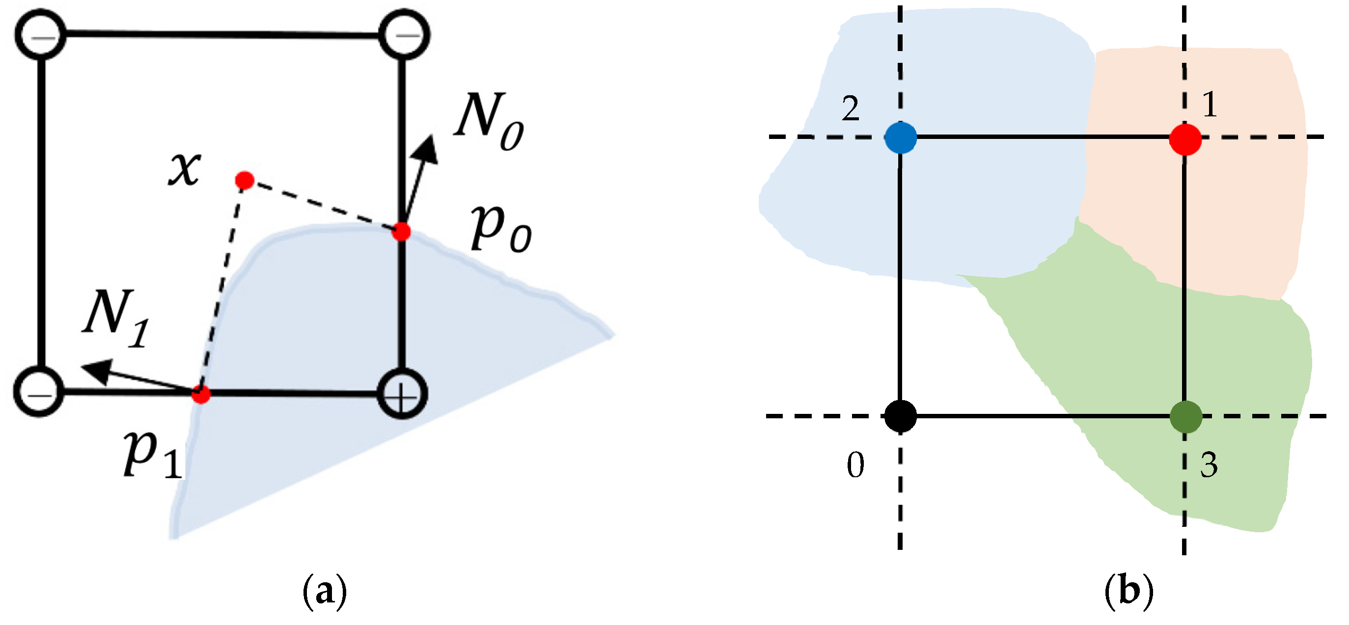
2.2.1. An Overview of the Single-Surface Dual Contouring Algorithm
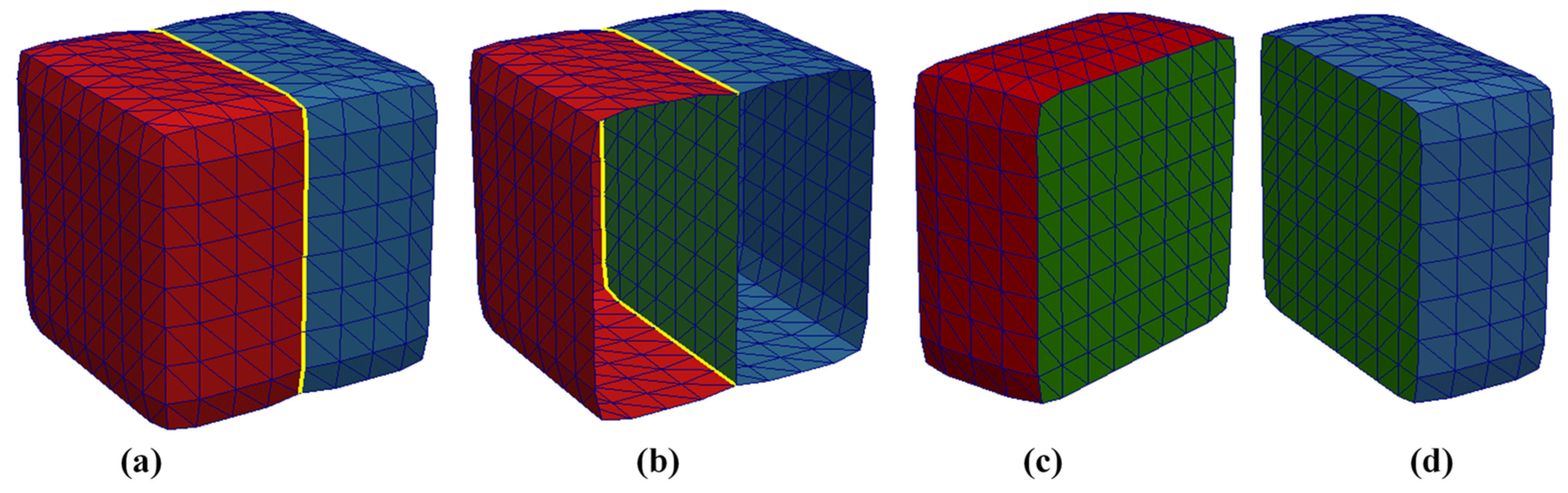
2.2.2. Multi-Material vs. Two-Manifold Contouring
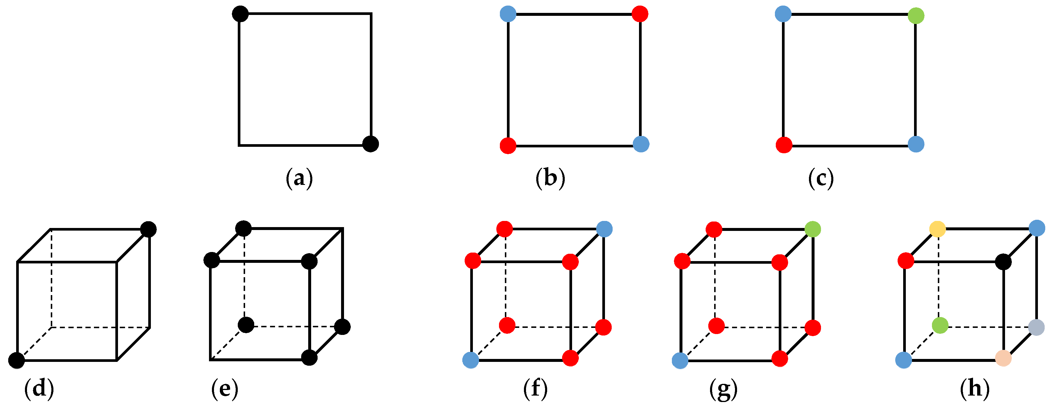
2.2.3. Ambiguous vs. Unambiguous Grid Cubes
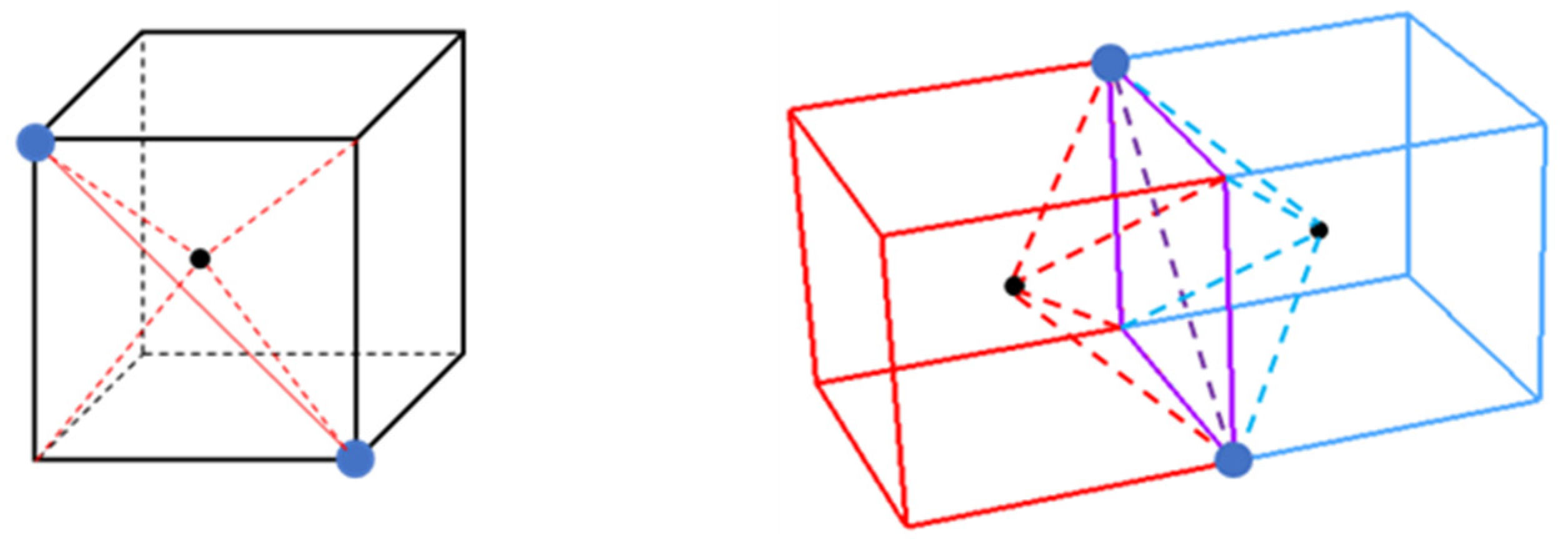
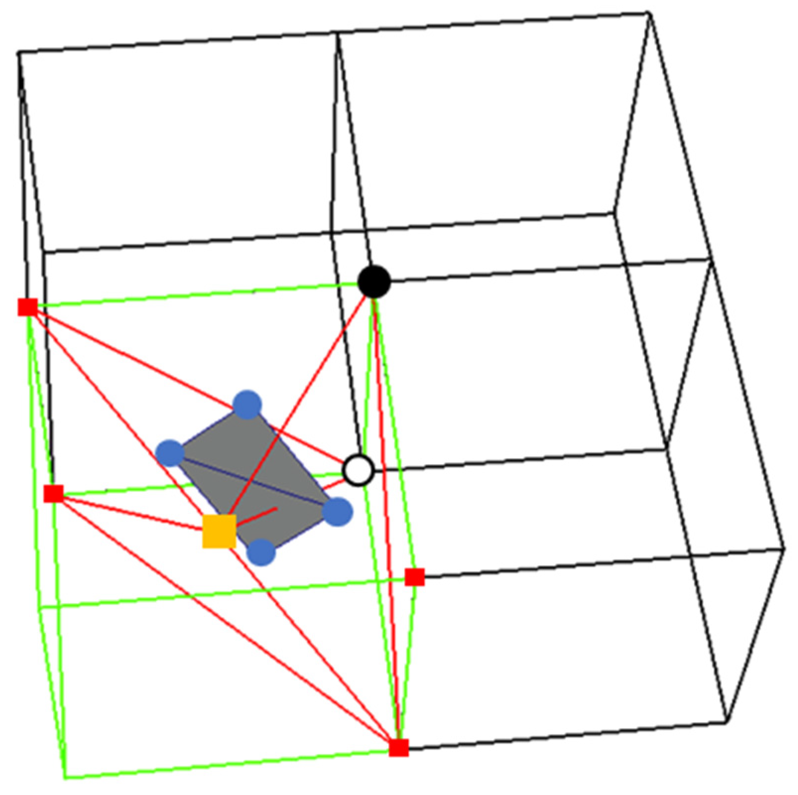
2.2.4. Tetrahedral Decomposition of Ambiguous Cubes
- If the two diagonally opposite corners are contiguous with each other through the interior of the volume, create a face diagonal between the two corners.
- If the two diagonally opposite corners are inside the volume but not contiguous with each other through the interior, create a face diagonal using the other two corners.
- For all other cases, any appropriate face diagonal can be used.
2.2.5. Polygon Generation
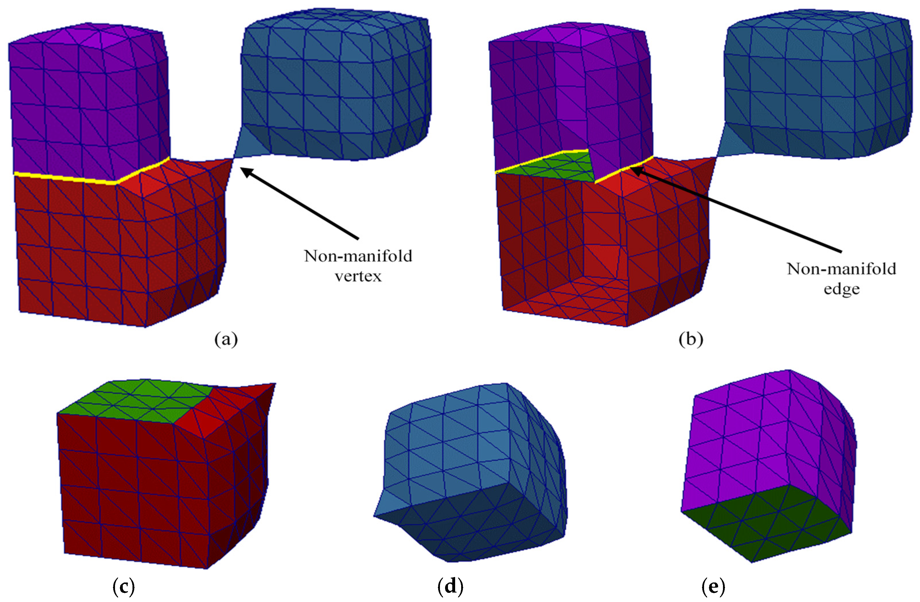
2.2.6. Verifying Two-Manifoldness and Quality of Multi-Material Meshes
2.3. Multi-Material Tetrahedral Mesh Generation
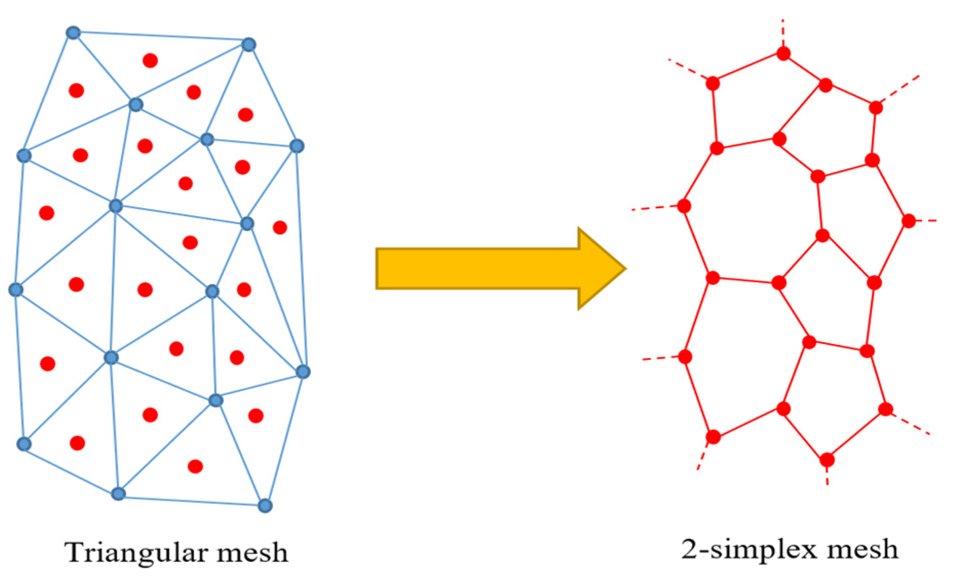
2.4. Deformable Multi-Surface Models
Initializing Multi-Material Two-Simplex Meshes
- Step 1: Compute the centroids of each triangle of the triangular mesh.
- Step 2: For each material index, perform the following:
- ○
- Step 2.1: For each ith vertex of the triangular mesh,
- ▪
- Step 2.1.1: Locate all the triangles with the current material index that contain the ith vertex;
- ▪
- Step 2.1.2: Use the centroids of these triangles to create one simplex cell.
3. Results
3.1. Multi-Material Surface Meshing
3.2. Multi-Material Tetrahedral Mesh Generation
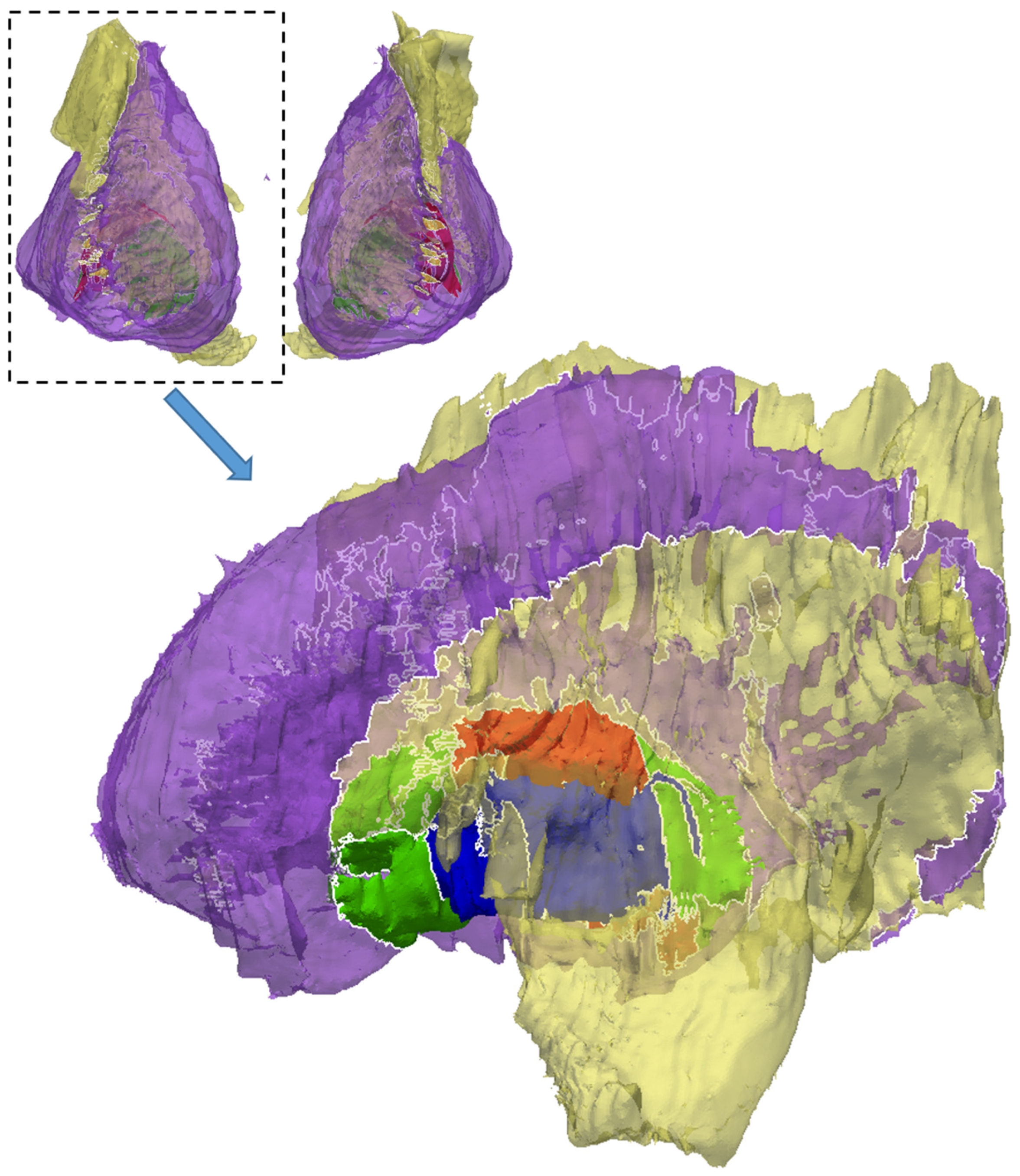
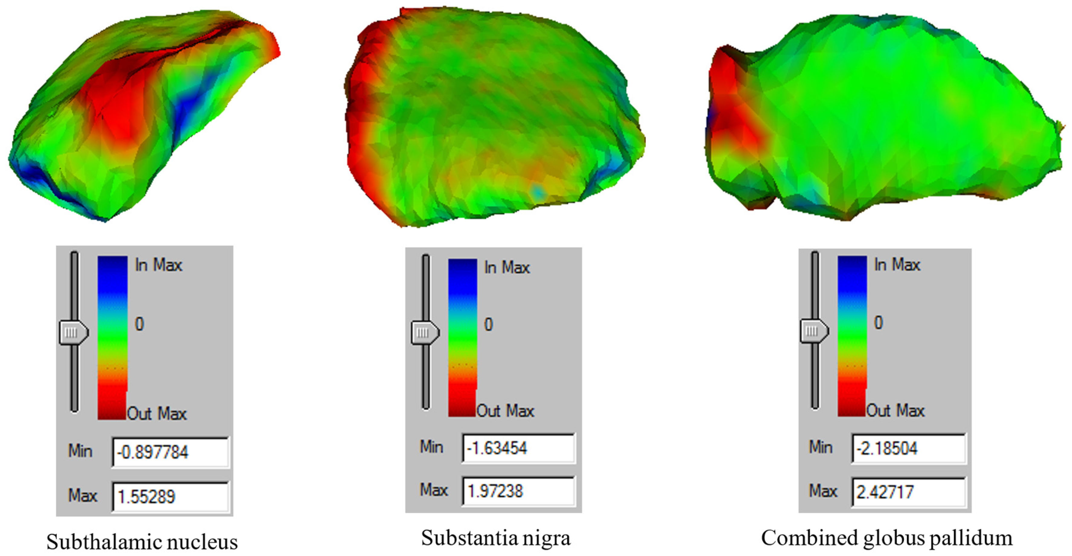
3.3. Deformable Multi-Surface Models
4. Discussion
5. Conclusions
Author Contributions
Funding
Data Availability Statement
Conflicts of Interest
References
- Richter, E.O.; Hoque, T.; Halliday, W.; Lozano, A.M.; Saint-Cyr, J.A. Determining the position and size of the subthalamic nucleus based on magnetic resonance imaging results in patients with advanced Parkinson disease. J. Neurosurg. 2004, 100, 541–546. [Google Scholar] [CrossRef] [PubMed]
- Hamani, C.; Florence, G.; Heinsen, H.; Plantinga, B.R.; Temel, Y.; Uludag, K.; Alho, E.; Teixeira, M.J.; Amaro, E.; Fonoff, E.T. Subthalamic nucleus deep brain stimulation: Basic concepts and novel perspectives. Eneuro 2017, 4, ENEURO.0140-17.2017. [Google Scholar] [CrossRef] [PubMed]
- Pham, D.L.; Xu, C.; Prince, J.L. Current methods in medical image segmentation. Annu. Rev. Biomed. Eng. 2000, 2, 315–337. [Google Scholar] [CrossRef] [PubMed]
- Litjens, G.; Kooi, T.; Bejnordi, B.E.; Setio, A.A.A.; Ciompim, F.; Ghafoorian, M.; van der Laak, J.A.W.M.; van Ginneken, B.; Sánchez, C.I. A survey on deep learning in medical image analysis. Med. Image Anal. 2017, 42, 60–88. [Google Scholar] [CrossRef]
- Sultana, S.; Blatt, J.E.; Gilles, B.; Rashid, T.; Audette, M.A. MRI-based Medial Axis Extraction and Boundary Segmentation of Cranial Nerves through Discrete Deformable 3D Contour and Surface Models. IEEE Trans. Med. Imaging 2017, 36, 1711–1721. [Google Scholar] [CrossRef]
- Gilles, B.; Magnenat-Thalmann, N. Musculoskeletal MRI segmentation using multi-resolution simplex meshes with medial representations. Med. Image Anal. 2010, 14, 291–302. [Google Scholar] [CrossRef]
- Lorensen, W.E.; Cline, H.E. Marching cubes: A high resolution 3D surface construction algorithm. ACM Siggraph Comput. Graph. 1987, 21, 163–169. [Google Scholar] [CrossRef]
- Ju, T.; Losasso, F.; Schaefer, S.; Warren, J. Dual contouring of hermite data. ACM Trans. Graph. (TOG) 2002, 339–346. Available online: https://pdfs.semanticscholar.org/6fb3/c8bd1d6f3d11f86e1863e9dd861ac128e964.pdf (accessed on 23 March 2023). [CrossRef]
- Treece, G.M.; Prager, R.W.; Gee, A.H. Regularised marching tetrahedra: Improved iso-surface extraction. Comput. Graph. 1999, 23, 583–598. [Google Scholar] [CrossRef]
- Szeliski, R.; Tonnesen, D.; Terzopoulos, D. Modeling surfaces of arbitrary topology with dynamic particles. In Computer Vision and Pattern Recognition, Proceedings of the CVPR’93, 1993 IEEE Computer Society Conference, New York, NY, USA, 15–18 June 1993; IEEE: New York, NY, USA, 1993. [Google Scholar]
- de Figueiredo, L.H.; Gomes, J.; Terzopoulos, D.; Velho, L. Physically-based methods for polygonization of implicit surfaces. In Proceedings of the Graphics Interface, Vancouver, BC, Canada, 11–15 May 1992. [Google Scholar]
- Bloomenthal, J.; Ferguson, K. Polygonization of non-manifold implicit surfaces. In Proceedings of the 22nd Annual Conference on Computer Graphics and Interactive Techniques, Los Angeles, CA, USA, 6–11 August 1995. [Google Scholar]
- Hege, H.-C.; Stalling, D.; Seebass, M.; Zöckler, M. A Generalized Marching Cubes Algorithm Based on Non-Binary; Citeseer: Princeton, NJ, USA, 1997. [Google Scholar]
- Bonnell, K.S.; Duchaineau, M.A.; Schikore, D.R.; Hamann, B.; Joy, K.I. Material interface reconstruction. IEEE Trans. Vis. Comput. Graph. 2003, 9, 500–511. [Google Scholar] [CrossRef]
- Wu, Z.; Sullivan, J.M. Multiple material marching cubes algorithm. Int. J. Numer. Methods Eng. 2003, 58, 189–207. [Google Scholar] [CrossRef]
- Reitinger, B.; Bornik, A.; Beichel, R. Constructing smooth non-manifold meshes of multi-labeled volumetric datasets. In Proceedings of the 13th International Conference in Central Europe on Computer Graphics, Visualization and Computer Vision 2005 in Co-Operation with EUROGRAPHICS, Plzen, Czech Republic, 31 January–4 February 2005. [Google Scholar]
- Bertram, M.; Reis, G.; van Lengen, R.H.; Köhn, S.; Hagen, H. Non-manifold Mesh Extraction from Time-varying Segmented Volumes used for Modeling a Human Heart. In Proceedings of the EuroVis 2005, Leeds, UK, 1–3 June 2005; pp. 199–206. [Google Scholar]
- Bischoff, S.; Kobbelt, L. Extracting consistent and manifold interfaces from multi-valued volume data sets. In Bildverarbeitung Für Die Medizin; Springer: Berlin, Germany, 2006; pp. 281–285. [Google Scholar]
- Boissonnat, J.-D.; Oudot, S. Provably good sampling and meshing of surfaces. Graph. Model. 2005, 67, 405–451. [Google Scholar] [CrossRef]
- Oudot, S.; Rineau, L.; Yvinec, M. Meshing volumes bounded by smooth surfaces. In Proceedings of the 14th International Meshing Roundtable, San Diego, CA, USA, 11–14 September 2005; Springer: Berlin, Germany, 2005. [Google Scholar]
- Pons, J.-P.; Ségonne, E.; Boissonnat, J.D.; Rineau, L.; Yvinec, M.; Keriven, R. High-quality consistent meshing of multi-label datasets. In Proceedings of the Biennial International Conference on Information Processing in Medical Imaging, Kerkrade, The Netherlands, 2–6 July 2007; Springer: Berlin, Germany, 2007. [Google Scholar]
- Zhang, Y.; Qian, J. Resolving topology ambiguity for multiple-material domains. Comput. Methods Appl. Mech. Eng. 2012, 247, 166–178. [Google Scholar] [CrossRef]
- Dillard, S.; Bingert, J.; Thoma, D.; Hamann, B. Construction of simplified boundary surfaces from serial-sectioned metal micrographs. IEEE Trans. Vis. Comput. Graph. 2007, 13, 1528–1535. [Google Scholar] [CrossRef]
- Meyer, M.; Whitaker, R.; Kirby, R.M.; Ledergerber, C.; Pfister, H. Particle-based sampling and meshing of surfaces in multimaterial volumes. Vis. Comput. Graph. IEEE Trans. 2008, 14, 1539–1546. [Google Scholar] [CrossRef] [PubMed]
- Rashid, T.; Sultana, S.; Audette, M.A. 2-manifold surface meshing using dual contouring with tetrahedral decomposition. Adv. Eng. Softw. 2016, 102, 83–96. [Google Scholar] [CrossRef]
- Li, B.; Christensen, G.E.; Hoffman, E.A.; McLennan, G.; Reinhardt, J.M. Establishing a normative atlas of the human lung: Intersubject warping and registration of volumetric CT images. Acad. Radiol. 2003, 10, 255–265. [Google Scholar] [CrossRef] [PubMed]
- Park, H.; Bland, P.H.; Meyer, C.R. Construction of an abdominal probabilistic atlas and its application in segmentation. Med. Imaging IEEE Trans. 2003, 22, 483–492. [Google Scholar] [CrossRef]
- Sluimer, I.; Prokop, M.; van Ginneken, B. Toward automated segmentation of the pathological lung in CT. Med. Imaging IEEE Trans. 2005, 24, 1025–1038. [Google Scholar] [CrossRef]
- Stancanello, J.; Romanelli, P.; Modugno, N.; Cerveri, P.; Ferrigno, G.; Uggeri, F.; Cantore, G. Atlas-based identification of targets for functional radiosurgery. Med. Phys. 2006, 33, 1603–1611. [Google Scholar] [CrossRef]
- Isgum, I.; Staring, M.; Rutten, A.; Prokop, M.; Viergever, M.A.; van Ginneken, B. Multi-atlas-based segmentation with local decision fusion—Application to cardiac and aortic segmentation in CT scans. Med. Imaging IEEE Trans. 2009, 28, 1000–1010. [Google Scholar] [CrossRef] [PubMed]
- Rohlfing, T.; Russakoff, D.B.; Maurer, C.R., Jr. Performance-based classifier combination in atlas-based image segmentation using expectation-maximization parameter estimation. Med. Imaging IEEE Trans. 2004, 23, 983–994. [Google Scholar] [CrossRef] [PubMed]
- Artaechevarria, X.; Munoz-Barrutia, A.; Ortiz-de-Solorzano, C. Combination strategies in multi-atlas image segmentation: Application to brain MR data. Med. Imaging IEEE Trans. 2009, 28, 1266–1277. [Google Scholar] [CrossRef] [PubMed]
- Sederberg, T.W.; Parry, S.R. Free-form deformation of solid geometric models. ACM Siggraph Comput. Graph. 1986, 151–160. [Google Scholar] [CrossRef]
- Terzopoulos, D.; Platt, J.; Barr, A.; Fleischer, K. Elastically deformable models. ACM Siggraph Comput. Graph. 1987, 205–214. [Google Scholar] [CrossRef]
- Meier, U.; López, O.; Monserrat, C.; Juan, M.C.; Alcañiz, M. Real-time deformable models for surgery simulation: A survey. Comput. Methods Programs Biomed. 2005, 77, 183–197. [Google Scholar] [CrossRef]
- Kass, M.; Witkin, A.; Terzopoulos, D. Snakes: Active contour models. Int. J. Comput. Vis. 1988, 1, 321–331. [Google Scholar] [CrossRef]
- Cootes, T.F.; Taylor, C.J.; Cooper, D.H.; Graham, J. Active shape models-their training and application. Comput. Vis. Image Underst. 1995, 61, 38–59. [Google Scholar] [CrossRef]
- Delingette, H. General object reconstruction based on simplex meshes. Int. J. Comput. Vis. 1999, 32, 111–146. [Google Scholar] [CrossRef]
- Delingette, H. Simplex meshes: A general representation for 3D shape reconstruction. In Computer Vision and Pattern Recognition, Proceedings of the CVPR’94, 1994 IEEE Computer Society Conference, Seattle, WS, USA, 16–18 May 1994; IEEE: New York, NY, USA, 1994. [Google Scholar]
- Delingette, H. Modélisation, Déformation et Reconnaissance D’objets Tridimensionnels à L’aide de Maillages Simplexes; Ecole Centrale Paris: Paris, France, 1994. [Google Scholar]
- Montagnat, J.; Delingette, H. Volumetric medical images segmentation using shape constrained deformable models. In CVRMed-MRCAS’97; Springer: Berlin, Germany, 1997. [Google Scholar]
- Gilles, B.; Moccozet, L.; Magnenat-Thalmann, N. Anatomical modelling of the musculoskeletal system from MRI. In Medical Image Computing and Computer-Assisted Intervention–MICCAI 2006; Springer: Berlin, Germany, 2006; pp. 289–296. [Google Scholar]
- Schmid, J.; Magnenat-Thalmann, N. MRI bone segmentation using deformable models and shape priors. In Medical Image Computing and Computer-Assisted Intervention–MICCAI 2008; Springer: Berlin, Germany, 2008; pp. 119–126. [Google Scholar]
- Schmid, J.; Iglesias Guitián, J.A.; Gobbetti, E.; Magnenat-Thalmann, N. A GPU framework for parallel segmentation of volumetric images using discrete deformable models. Vis. Comput. 2011, 27, 85–95. [Google Scholar] [CrossRef]
- Schmid, J.; Sandholm, A.; Chung, F.; Thalmann, D.; Delingette, H.; Magnenat-Thalmann, N. Musculoskeletal simulation model generation from MRI data sets and motion capture data. In Recent Advances in the 3D Physiological Human; Springer: Berlin, Germany, 2009; pp. 3–19. [Google Scholar]
- Montagnat, J.; Delingette, H. Space and time shape constrained deformable surfaces for 4D medical image segmentation. In Medical Image Computing and Computer-Assisted Intervention–MICCAI 2000; Springer: Berlin, Germany, 2000. [Google Scholar]
- Montagnat, J.; Delingette, H. 4D deformable models with temporal constraints: Application to 4D cardiac image segmentation. Med. Image Anal. 2005, 9, 87–100. [Google Scholar] [CrossRef] [PubMed]
- Montagnat, J.; Sermesant, M.; Delingette, H.; Malandain, G.; Ayache, N. Anisotropic filtering for model-based segmentation of 4D cylindrical echocardiographic images. Pattern Recognit. Lett. 2003, 24, 815–828. [Google Scholar] [CrossRef]
- Cremers, D.; Schnorr, C.; Weickert, J. Diffusion-snakes: Combining statistical shape knowledge and image information in a variational framework. In Variational and Level Set Methods in Computer Vision, Proceedings of the IEEE Workshop on Variational and Level Set Methods in Computer Vision, Vancouver, BC, Canada, 13 July 2001; IEEE: New York, NY, USA, 2001. [Google Scholar]
- Cremers, D.; Schnörr, C.; Weickert, J.; Schellewald, C. Diffusion–snakes using statistical shape knowledge. In Algebraic Frames for the Perception-Action Cycle; Springer: Berlin, Germany, 2000; pp. 164–174. [Google Scholar]
- Cremers, D.; Tischhäuser, F.; Weickert, J.; Schnörr, C. Diffusion snakes: Introducing statistical shape knowledge into the Mumford-Shah functional. Int. J. Comput. Vis. 2002, 50, 295–313. [Google Scholar] [CrossRef]
- Haq, R.; Aras, R.; Besachio, D.A.; Borgie, R.C.; Audette, M.A. 3D lumbar spine intervertebral disc segmentation and compression simulation from MRI using shape-aware models. Int. J. Comput. Assist. Radiol. Surg. 2015, 10, 45–54. [Google Scholar] [CrossRef] [PubMed]
- Haq, R.; Besachio, D.A.; Borgie, R.C.; Audette, M.A. Using shape-aware models for lumbar spine intervertebral disc segmentation. In Pattern Recognition (ICPR), Proceedings of the 22nd International Conference on Pattern Recognition, Stockholm, Sweden, 24–28 August 2014; IEEE: New York, NY, USA, 2014. [Google Scholar]
- Haq, R.; Cates, J.E.; Besachio, D.A.; Borgie, R.C.; Audette, M.A. Statistical Shape Model Construction of Lumbar Vertebrae and Intervertebral Discs in Segmentation for Discectomy Surgery Simulation. In International Workshop on Computational Methods and Clinical Applications for Spine Imaging; Springer: Berlin, Germany, 2015. [Google Scholar]
- Sultana, S.; Blatt, J.E.; Lee, Y.; Ewend, M.; Cetas, J.; Costa, A.; Audette, M.A. Patient-specific cranial nerve identification using a discrete deformable contour model for skull base neurosurgery planning and simulation. In Workshop on Clinical Image-Based Procedures; Springer: Berlin, Germany, 2015. [Google Scholar]
- Golub, G.H.; Van Loan, C.F. Matrix Computations. In Johns Hopkins Series in the Mathematical Sciences; Johns Hopkins University Press: Baltimore, MD, USA, 1989. [Google Scholar]
- Kobbelt, L.P.; Botsch, M.; Schwanecke, U.; Seidel, H.P. Feature sensitive surface extraction from volume data. In Proceedings of the 28th Annual Conference on Computer Graphics and Interactive Techniques, Los Angeles, CA, USA, 12–17 August 2001; ACM: New York, NY, USA, 2001. [Google Scholar]
- Lindstrom, P. Out-of-core simplification of large polygonal models. In Proceedings of the 27th Annual Conference on Computer Graphics and Interactive Techniques, New Orleans, LA, USA, 23–28 July 2000; ACM Press: New York, NY, USA; Addison-Wesley Publishing Co.: Boston, MA, USA, 2000. [Google Scholar]
- Zhang, Y.; Qian, J. Dual Contouring for domains with topology ambiguity. Comput. Methods Appl. Mech. Eng. 2012, 217–220, 34–45. [Google Scholar] [CrossRef]
- Sohn, B.-S. Topology preserving tetrahedral decomposition of trilinear cell. In Computational Science–ICCS 2007; Springer: Berlin, Germany, 2007; pp. 350–357. [Google Scholar]
- CGAL Editorial Board. The CGAL Project, CGAL User and Reference Manual, 4.13 ed.; CGAL Editorial Board: Glasgow, UK, 2018. [Google Scholar]
- Cignoni, P.; Callieri, M.; Corsini, M.; Dellepiane, M.; Ganovelli, F.; Ranzuglia, G. Meshlab: An open-source mesh processing tool. In Proceedings of the Eurographics Italian Chapter Conference, Salerno, Italy, 2–4 July 2008. [Google Scholar]
- Shewchuk, J. What is a Good Linear Finite Element? Interpolation, Conditioning, Anisotropy, and Quality Measures (Preprint); University of California at Berkeley: Berkeley, CA, USA, 2002. [Google Scholar]
- Chakravarty, M.M.; Bertrand, G.; Hodge, C.P.; Sadikot, A.F.; Collins, D.L. The creation of a brain atlas for image guided neurosurgery using serial histological data. Neuroimage 2006, 30, 359–376. [Google Scholar] [CrossRef]
- Owen, S.J. A survey of unstructured mesh generation technology. IMR 1998, 239, 267. [Google Scholar]
- Si, H. TetGen, a Delaunay-based quality tetrahedral mesh generator. ACM Trans. Math. Softw. (TOMS) 2015, 41, 11. [Google Scholar] [CrossRef]
- CGAL Editorial Board. The CGAL Project, CGAL User and Reference Manual, 4.9 ed.; CGAL Editorial Board: Glasgow, UK, 2016. [Google Scholar]
- O’Gorman, R.L.; Shmueli, K.; Ashkan, K.; Samuel, M.; Lythgoe, D.J.; Shahidiani, A.; Wastling, S.J.; Footman, M.; Selway, R.P.; Jarosz, J. Optimal MRI methods for direct stereotactic targeting of the subthalamic nucleus and globus pallidus. Eur. Radiol. 2011, 21, 130–136. [Google Scholar] [CrossRef] [PubMed]
- Wang, B.T.; Poirier, S.; Guo, T.; Parrent, A.G.; Peters, T.M.; Khan, A.R. Generation and evaluation of an ultra-high-field atlas with applications in DBS planning. In SPIE Medical Imaging; International Society for Optics and Photonics: Bellingham, WS, USA, 2016. [Google Scholar]
- Tapp, A.; Payer, C.; Schmid, J.; Polanco, M.; Kumi, I.; Bawab, S.; Ringleb, S.; St. Remy, C.; Bennett, J.; Kakar, R.S.; et al. Generation of Patient-Specific, Ligamentoskeletal, Finite Element Meshes for Scoliosis Correction Planning. CLIP/DCL/LL-COVID19/PPML@MICCAI 2021; Springer International Publishing: New York, NY, USA, 2021; pp. 13–23. [Google Scholar]
- Zhang, D.; Yao, L.; Chen, K.; Wang, S.; Chang, X.; Liu, Y. Making Sense of Spatio-Temporal Preserving Representations for EEG-Based Human Intention Recognition. IEEE Trans. Cybern. 2020, 50, 3033–3044. [Google Scholar] [CrossRef]
- Luo, M.; Chang, X.; Nie, L.; Yang, Y.; Hauptmann, A.G.; Zheng, Q.Q. An Adaptive Semisupervised Feature Analysis for Video Semantic Recognition. IEEE Trans. Cybern. 2018, 48, 648–660. [Google Scholar] [CrossRef] [PubMed]
- Sultana, S.; Agrawal, P.; Elhabian, S.Y.; Whitaker, R.T.; Rashid, T.; Blatt, J.E.; Cetas, J.S.; Audette, M.A. Towards a Statistical Shape-Aware Deformable Contour Model for Cranial Nerve Identification. In Workshop on Clinical Image-Based Procedures; Springer: Berlin, Germany, 2016. [Google Scholar]
- de Rochefort, L.; Liu, T.; Kressler, B.; Liu, J.; Spincemaille, P.; Lebon, V.; Wu, J.; Wang, Y. Quantitative susceptibility map reconstruction from MR phase data using bayesian regularization: Validation and application to brain imaging. Magn. Reson. Med. 2010, 63, 194–206. [Google Scholar] [CrossRef] [PubMed]
- Liu, T.; Eskreis-Winkler, S.; Schweitzer, A.D.; Chen, W.; Kaplitt, M.G.; Tsiouris, A.J.; Wang, Y. I Improved subthalamic nucleus depiction with quantitative susceptibility mapping. Radiology 2013, 269, 216–223. [Google Scholar] [CrossRef]
- Wang, Y.; Liu, T. Quantitative susceptibility mapping (QSM): Decoding MRI data for a tissue magnetic biomarker. Magn. Reson. Med. 2015, 73, 82–101. [Google Scholar] [CrossRef] [PubMed]
- Xiao, Y.; Beriault, S.; Pike, G.B.; Collins, D.L. Multicontrast multiecho FLASH MRI for targeting the subthalamic nucleus. Magn. Reson. Imaging 2012, 30, 627–640. [Google Scholar] [CrossRef] [PubMed]
- Rashid, T.; Sultana, S.; Fischer, G.S.; Pilitsis, J.; Audette, M.A. Deformable Multi-Material 2-Simplex Surface Mesh for Intraoperative MRI-Ready Surgery Planning and Simulation, with Deep-Brain Stimulation Applications; Cardoso, M.J., Arbel, T., Tavares, J.M.R.S., Aylward, S., Li, S., Boctor, E., Fichtinger, G., Cleary, K., Freeman, K.B., Kohli, L., et al., Eds.; MICCAI BIVPCS/POCUS-2017. LNCS; Springer: Berlin, Germany, 2017; Volume 10549, pp. 94–102. [Google Scholar]


| Atlas Label | Structure Name | Number of Triangles | Number of Vertices | Average Radius Ratio (Worst Value) | |
|---|---|---|---|---|---|
| Figure 16 | Whole mesh | 1,672,483 | 813,209 | 0.8104 (0.0917) | |
| Figure 17a | 1 | Striatum | 842,266 | 419,399 | 0.8044 (0.0921) |
| Figure 17b | 4 | Internal capsule | 1,023,284 | 509,696 | 0.8082 (0.0966) |
| Figure 17c | 5 | Globus pallidus | 76,120 | 38,010 | 0.8083 (0.1192) |
| Figure 17d | 11 | Globus pallidus internal | 73,008 | 36,382 | 0.8008 (0.1148) |
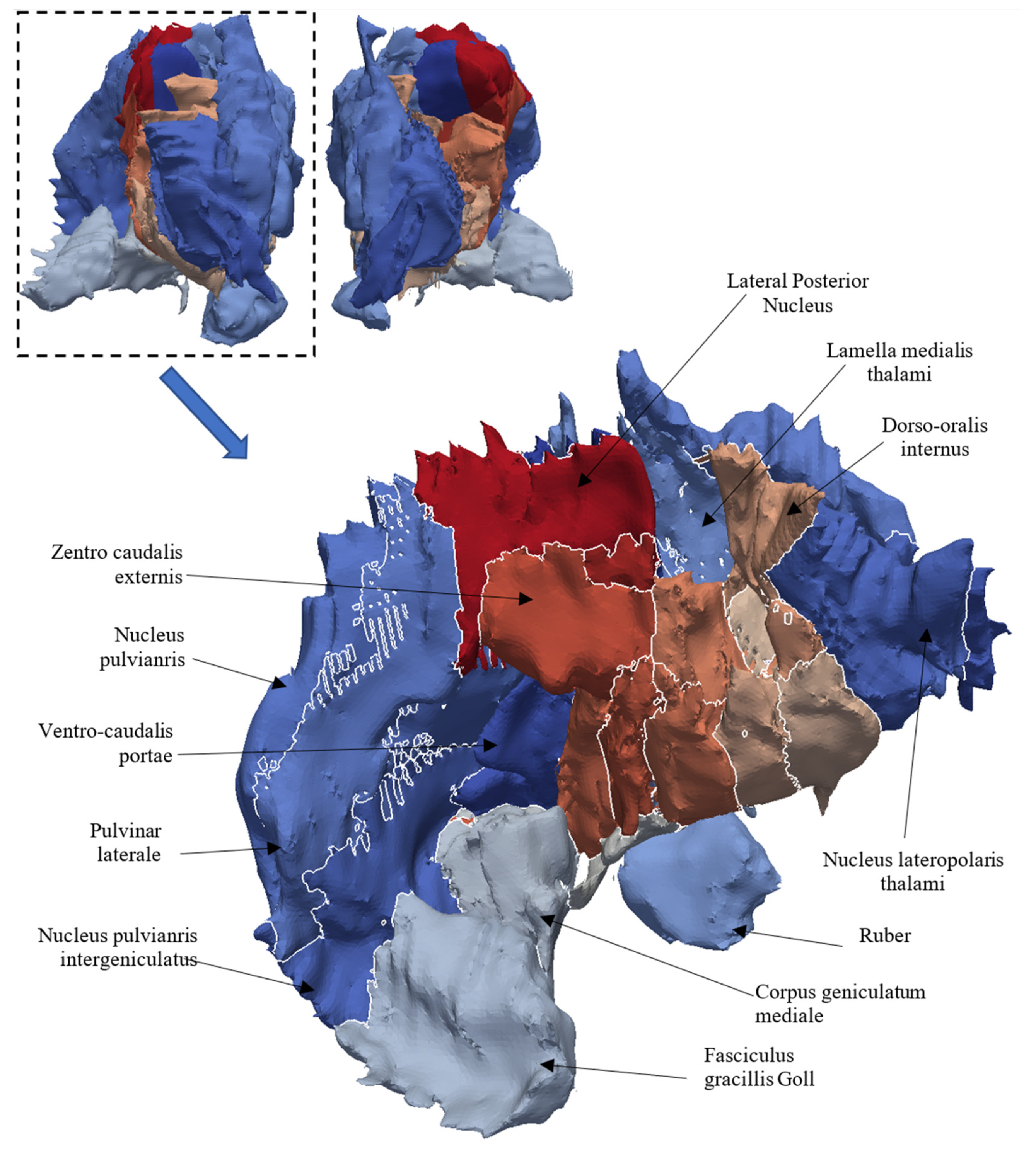
| Atlas Label | Structure Name | Number of Triangles | Number of Vertices | Average Radius Ratio (Worst Ratio) |
|---|---|---|---|---|
| Whole Mesh | 656,909 | 307,226 | 0.8101 (0.0394) | |
| 22 | Stria medullaris thalami (st. m) | 6044 | 3030 | 0.8357 (0.1240) |
| 26 | Nucleus lateropolaris thalami (Lpo) | 39,404 | 19,638 | 0.8062 (0.1324) |
| 27 | Nucleus fasciculosus thalami (Fa) | 13,116 | 6552 | 0.8257 (0.1142) |
| 28 | Nucleus anterior principalis (Apr) | 22,276 | 11,144 | 0.8299 (0.0730) |
| 37 | Nucleus medialis (M) | 80,866 | 40,417 | 0.8135 (0.1088) |
| 40 | Lamella medialis thalami (La. M.) | 66,876 | 33,242 | 0.7932 (0.0795) |
| 48 | Ruber (Ru) | 14,754 | 7349 | 0.8317 (0.1928) |
| 49 | Nucleus Centralis (Ce.) | 41,260 | 20,566 | 0.7923 (0.0885) |
| 51 | Nucleus parafasicular (Pf.) | 21,654 | 10,769 | 0.7746 (0.0885) |
| 60 | Fasciculus gracilis Goll (G) | 24,230 | 11,995 | 0.8155 (0.1313) |
| 68 | Corpus geniculatum mediale (G.m) | 41,182 | 20,541 | 0.8162 (0.1722) |
| 70 | Nucleus Limitans (Li) | 20,548 | 10,266 | 0.8233 (0.1675) |
| 71 | Ventro-caudalis parvocell. (V.c.pc) | 9646 | 4825 | 0.8171 (0.2153) |
| 81 | Ventro-oralis medialis (V.o.m.) | 7644 | 3824 | 0.8089 (0.1467) |
| 86 | Ventro-oralis internus (V.o.i.) | 22,450 | 11,147 | 0.8033 (0.1008) |
| 87 | Ventro-oralis anterior (V.o.a) | 26,216 | 12,956 | 0.7827 (0.0835) |
| 88 | Ventro-oralis posterior (V.o.p.) | 18,254 | 9019 | 0.8024 (0.1338) |
| 89 | Dorso-oralis internus (D.o.i) | 18,998 | 9391 | 0.7945 (0.1200) |
| 90 | Zentrolateralis oralis (Z.o.) | 4346 | 2137 | 0.7715 (0.0394) |
| 91 | Ventro-intermedius internus (V.im.i) | 20,196 | 9980 | 0.7889 (0.1410) |
| 92 | Zentro-lateralis externus (Z.im.e) | 12,268 | 6022 | 0.8000 (0.1048) |
| 94 | Ventro-intermedius externus (V.im.e) | 23,382 | 11,559 | 0.7994 (0.1088) |
| 95 | Ventro-caudalis internus (V.c.i) | 23,364 | 11,566 | 0.7950 (0.1505) |
| 96 | Ventro-caudalis anterior internus (V.c.a.e) | 12,282 | 6105 | 0.8109 (0.1134) |
| 97 | Zentro caudalis externis (Z.c.e) | 15,438 | 7675 | 0.8217 (0.1512) |
| 98 | Zentro caudalis internis (Z.c.i) | 8868 | 4420 | 0.8168 (0.0999) |
| 99 | Dorso-caudalis (D.c.) | 3882 | 1929 | 0.8092 (0.1426) |
| 100 | Nucleus pulvinaris orolateralis (Pu.o.l.) | 34,254 | 16,981 | 0.8172 (0.1105) |
| 101 | Nucleus pulvinaris oromedialis (Pu.o.m.) | 26,330 | 13,079 | 0.8057 (0.1218) |
| 102 | Ventro-caudalis portae (V.c.por) | 25,636 | 12,734 | 0.8220 (0.1036) |
| 104 | Nucleus ventroimtermedius internus (V.im.i) | 4146 | 2055 | 0.7847 (0.1412) |
| 105 | Nucleus pulvinaris intergeniculatus (Pu.ig) | 35,768 | 17,562 | 0.7929 (0.1091) |
| 106 | Nucleus pulvinaris (Pu.m) | 86,364 | 43,020 | 0.8277 (0.1036) |
| 107 | Pulvinar laterale (Pu.l) | 37,448 | 18,440 | 0.7925 (0.1444) |
| Anatomical Structures | Hausdorff Distance | Mean Square Distance (MSD) | Mean Absolute Distance (MAD) | Dice’s Coefficient |
|---|---|---|---|---|
| Subthalamic nucleus | 2.10539 | 0.30867 | 0.35002 | 0.773219 |
| Substantia nigra | 2.54666 | 0.357749 | 0.455244 | 0.799318 |
| Globus pallidum | 2.42717 | 0.216618 | 0.307724 | 0.927084 |
Disclaimer/Publisher’s Note: The statements, opinions and data contained in all publications are solely those of the individual author(s) and contributor(s) and not of MDPI and/or the editor(s). MDPI and/or the editor(s) disclaim responsibility for any injury to people or property resulting from any ideas, methods, instructions or products referred to in the content. |
© 2023 by the authors. Licensee MDPI, Basel, Switzerland. This article is an open access article distributed under the terms and conditions of the Creative Commons Attribution (CC BY) license (https://creativecommons.org/licenses/by/4.0/).
Share and Cite
Rashid, T.; Sultana, S.; Chakravarty, M.; Audette, M.A. Atlas-Based Shared-Boundary Deformable Multi-Surface Models through Multi-Material and Two-Manifold Dual Contouring. Information 2023, 14, 220. https://doi.org/10.3390/info14040220
Rashid T, Sultana S, Chakravarty M, Audette MA. Atlas-Based Shared-Boundary Deformable Multi-Surface Models through Multi-Material and Two-Manifold Dual Contouring. Information. 2023; 14(4):220. https://doi.org/10.3390/info14040220
Chicago/Turabian StyleRashid, Tanweer, Sharmin Sultana, Mallar Chakravarty, and Michel Albert Audette. 2023. "Atlas-Based Shared-Boundary Deformable Multi-Surface Models through Multi-Material and Two-Manifold Dual Contouring" Information 14, no. 4: 220. https://doi.org/10.3390/info14040220
APA StyleRashid, T., Sultana, S., Chakravarty, M., & Audette, M. A. (2023). Atlas-Based Shared-Boundary Deformable Multi-Surface Models through Multi-Material and Two-Manifold Dual Contouring. Information, 14(4), 220. https://doi.org/10.3390/info14040220