Abstract
Normalization as a layer within neural networks has over the years demonstrated its effectiveness in neural network optimization across a wide range of different tasks, with one of the most successful approaches being that of batch normalization. The consensus is that better estimates of the BatchNorm normalization statistics ( and ) in each mini-batch result in better optimization. In this work, we challenge this belief and experiment with a new variant of BatchNorm known as GhostNorm that, despite independently normalizing batches within the mini-batches, i.e., and are independently computed and applied to groups of samples in each mini-batch, outperforms BatchNorm consistently. Next, we introduce sequential normalization (SeqNorm), the sequential application of the above type of normalization across two dimensions of the input, and find that models trained with SeqNorm consistently outperform models trained with BatchNorm or GhostNorm on multiple image classification data sets. Our contributions are as follows: (i) we uncover a source of regularization that is unique to GhostNorm, and not simply an extension from BatchNorm, and illustrate its effects on the loss landscape, (ii) we introduce sequential normalization (SeqNorm) a new normalization layer that improves the regularization effects of GhostNorm, (iii) we compare both GhostNorm and SeqNorm against BatchNorm alone as well as with other regularization techniques, (iv) for both GhostNorm and SeqNorm models, we train models whose performance is consistently better than our baselines, including ones with BatchNorm, on the standard image classification data sets of CIFAR–10, CIFAR-100, and ImageNet ((, , ), and (, , ) for GhostNorm and SeqNorm, respectively).
1. Introduction
The effectiveness of batch normalization (BatchNorm), a technique first introduced by Ioffe and Szegedy [1] on neural network (NN) optimization, has been demonstrated over the years on a variety of tasks, including computer vision [2,3,4], speech recognition [5], and other [6,7,8]. BatchNorm is typically embedded at each NN layer either before or after the activation function, normalizing and projecting the input features to match a Gaussian-like distribution. Consequently, the activation values of each layer maintain more stable distributions during NN training, which in turn is thought to enable faster convergence and better generalization performance [1,9,10]. Following the effectiveness of BatchNorm on NN optimization, other normalization techniques emerged [11,12,13,14,15], a number of which introduced normalization across a different input dimension (e.g., layer normalization [12]), while others focused on improving other aspects of BatchNorm, such as the accuracy of the batch statistics estimates [11,16,17], or the train–test discrepancy in BatchNorm use [18].
Despite the wide adoption and practical success of BatchNorm, its underlying mechanics within the context of NN optimization has yet to be fully understood. Initially, Ioeffe and Szegedy suggested that it came from it reducing the so-called internal covariate shift [1]. At a high level, internal covariate shift refers to the change in the distribution of the inputs of each NN layer that is caused by updates to the previous layers. This continual change throughout training was conjectured to negatively affect optimization [1,9]. However, recent research disputes that with compelling evidence that demonstrates how BatchNorm may in fact be increasing the internal covariate shift [9]. Instead, the effectiveness of BatchNorm is argued to be a consequence of a smoother loss landscape [9]. In our present work, we began with a novel analysis of the effects on the loss landscape [9] between BatchNorm and Ghost normalization (GhostNorm) on MNIST and CIFAR-10 data sets. GhostNorm can be thought as an extension to BatchNorm, as GroupNorm is to LayerNorm (illustrated in Figure 1). In particular, in GhostNorm, the initial batch is divided into a number of smaller batches (also called “ghost” batches), each normalized independently of the other [19]. GhostNorm goes against the popular belief that associates the degradation in BatchNorm performance with smaller batch sizes to poorer estimates of mean and variance due to having a smaller sample size [11,14,20]. We observed that although GhostNorm decreased the smoothness of the loss landscape when compared to BatchNorm, models trained with GhostNorm across a range of batch sizes (4 to 32 and in later experiments, up to 512), and ghost batch sizes, consistently outperformed BatchNorm alternatives. Our experimental results corroborate our hypothesis that GhostNorm has a fundamentally different, yet better, effect on NN optimization when compared to BatchNorm. Finally, we used the insights revealed by our analysis to propose a new type of normalization, which we term sequential normalization (SeqNorm).
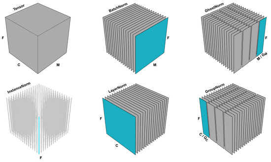
Figure 1.
The input tensor with dimensions is divided into a number of line (1D) or plane (2D) slices. Each normalization technique slices the input tensor differently and each slice is normalized independently of the other slices. For ease of visualization, both and are set to 4.
The contributions of this paper are as follows: (i) we introduce different ways of employing GhostNorm as a normalization layer, (ii) we identify a source of regularization in GhostNorm that cannot be found in any of the existing alternatives, (iii) we visualize the loss landscape of GhostNorm under vastly different experimental setups, and observe that GhostNorm consistently decreases the smoothness of the loss landscape, especially on the later epochs of training, while outperforming BatchNorm alternatives, (iv) we introduce a new normalization layer called SeqNorm that adopts the GhostNorm approach to normalization sequentially over more input dimensions, (v) we demonstrate consistently better generalization performances on CIFAR-10, CIFAR-100, and ImageNet when BatchNorm is replaced with either GhostNorm or SeqNorm, with the latter surpassing the SOTA on CIFAR-100 and ImageNet.
The rest of the paper is organized as follows. In Section 1.1, we discuss the related work for both GhostNorm and SeqNorm. In Section 2, we formulate the existing layer normalization techniques as well as the key novelty of the present work, SeqNorm, highlight the differences, and provide implementation details for both GhostNorm and SeqNorm. In Section 3, we first conduct experiments to visualize the loss landscape of GhostNorm, a component which has been described as the primary reason behind the effectiveness of BatchNorm, and then train models for image classification on CIFAR-10, CIFAR-100, and ImageNet. This section, alongside Appendix B and Appendix C, provides reproducibility information for all conducted experiments. Finally, we conclude our work with a discussion of our experimental results in Section 4.
1.1. Related Work
Ghost normalization is a technique originally introduced by Hoffer et al. [19]. Over the years, the primary use of GhostNorm has been to optimize NNs with large batch sizes over multiple GPUs [21]. Unfortunately, when compared to other normalization techniques [11,12,13,14,15], the adoption of GhostNorm has been rather scarce, and narrow to large batch size training regimes [21,22,23,24]. More recently, GhostNorm has been used over BatchNorm as a means of regulating the amount of noise that arises from the estimation of the normalization statistics for increasingly larger batch sizes [22,23,24]. This was achieved by keeping the ghost batch size constant [19].
Closest in spirit to the present work is the recent research by Summers and Dinneen [21], who experimented with GhostNorm on both small and medium batch size training regimes. Summers and Dinneen [21] tuned the number of groups within GhostNorm (see Section 2.1) on CIFAR-100, Caltech-256, and SVHN, and reported positive results on the first two data sets. More results are reported on other data sets through transfer learning. However, the use of other new optimization methods confounds the attribution of the observed improvement.
The closest line of work to SeqNorm is, again, found in the work of Summers and Dinneen [21]. Therein, they employed a normalization technique which although at first glance may appear similar to SeqNorm, it is fundamentally different. This stems from the vastly different goals between our works, i.e., Summers and Dinneen tried to improve layer normalization for small batch sizes [21], whereas we strive to improve layer normalization in a more general setting. At a high level, where SeqNorm performs GroupNorm and GhostNorm sequentially, their normalization method applies both simultaneously. At a fundamental level, the normalization layer that was used by Summers and Dinneen embeds the stochastic nature of GhostNorm into that of GroupNorm (see Section 2.2), thereby potentially disrupting the learning of channel grouping within NNs. Other works that apply simultaneous normalization strategies include that of Bronskill et al. [25], who blended the moments of BatchNorm with InstanceNorm or LayerNorm, as well as Luo et al. [26], who introduced switchable normalization—a layer that enables the NN to learn which normalization techniques to employ at different layers.
2. Methodology
2.1. Formulation
Given a fully connected or convolutional neural network, the parameters of a typical layer l with normalization, , are the weights as well as the scale and shift parameters and . For brevity, we omit the l superscript. Given an input tensor X, the activation values A of layer l are computed as
where is the activation function, ⊙ corresponds to either matrix multiplication or convolution for fully connected and convolutional layers respectively, and ⊗ describes an element-wise multiplication.
Most normalization techniques differ in how they transform the product . Let the product be a tensor with dimensions, where M is the so-called mini-batch size, or just batch size, C is the channels dimension, and F is the spatial dimension.
In BatchNorm [1], the given tensor is normalized across the channels dimension. In particular, the mean and variance are computed across C number of slices of dimensions (see Figure 1), which are subsequently used to normalize each channel independently. In LayerNorm [12], statistics are computed over M slices, each having the dimension , normalizing the values of each data sample independently. InstanceNorm [15] normalizes the values of the tensor over both M and C, i.e., computes statistics across slices of F dimension.
GroupNorm [14] can be thought as an extension to LayerNorm, wherein the C dimension is divided into number of groups, i.e., . Statistics are calculated over slices of dimensions. Similarly, GhostNorm can be thought as an extension to BatchNorm, wherein the M dimension is divided into groups, normalizing over slices of dimensions. Both and are hyperparameters that can be tuned based on a validation set. All of the aforementioned normalization techniques are illustrated in Figure 1.
SeqNorm can be thought as the employment of GroupNorm and GhostNorm sequentially. Initially, the input tensor is divided into dimensions, normalizing across number of slices, i.e., same as GroupNorm. Then, once the and dimensions are collapsed back together, the input tensor is divided into dimensions for normalizing over slices of dimensions, i.e., same as GhostNorm.
Any of the slices described above is treated as a set of values S with one dimension. The mean and variance of S are computed in the traditional way (see Equation (2)). The values of S are then normalized as shown below.
Once all slices are normalized, the output of the layer is simply the concatenation of all slices back into the initial tensor shape.
2.2. The Effects of Ghost Normalization
There is only one other published work which has investigated the effectiveness of ghost normalization for small and medium mini-batch sizes [21]. Therein, the authors hypothesized that GhostNorm offers stronger regularization than BatchNorm, as it computes the normalization statistics on smaller sample sizes [21]. In this section, we support that hypothesis by providing insights into a particular source of regularization, unique to GhostNorm, that stems from the normalization of activations in independent groups and with different statistics.
Consider as an example the tuple X with values, which can be thought as an input tensor with dimensions. Given to a BatchNorm layer, the output is the normalized version with values . Note how although the values have changed, the ranking order of the activation values has remained the same, e.g., the 2nd value is larger than the 5th value in both X () and (). More formally, the following holds true:
On the other hand, given X to a GhostNorm layer with , the output is . Now, we observe that after normalization, the 2nd value has become much smaller than the 5th value in (). Where BatchNorm preserves the ranking order of the received activations, GhostNorm can end up modifying their values, and hence alter the course of optimization. Our experimental results demonstrate how GhostNorm improves upon BatchNorm, supporting the hypothesis that the above type of regularization can be beneficial to optimization. Note that for BatchNorm, the condition in Equation (4) only holds true across the dimension of the input tensor, whereas for GhostNorm it cannot be guaranteed for any dimension.
2.2.1. GhostNorm to BatchNorm
One can argue that the same type of regularization can be found in BatchNorm over different mini-batches, e.g., given and as two different mini-batches. However, GhostNorm introduces the above during each forward pass rather than between forward passes. Hence, it is a regularization that is embedded during learning (GhostNorm), rather than across learning (BatchNorm).
2.2.2. GhostNorm to GroupNorm
Despite the visual symmetry between GhostNorm and GroupNorm, there is one major difference. Grouping has been employed extensively in classical feature engineering, such as SIFT, HOG, and GIST, wherein independent normalization is often performed over these groups [14]. At a high level, GroupNorm can be thought as motivating the network to group similar features together [14]. However, for GhostNorm, this would not be possible due to random sampling, and random arrangement of the data within each mini-batch. Therefore, we hypothesize that the effects of these two normalization techniques could be combined for their benefits to be accumulated. Specifically, we propose SeqNorm, a normalization technique that employs both GroupNorm and GhostNorm in a sequential manner. SeqNorm can also be thought as a natural extension to GhostNorm that allows smaller sample size normalization on more input dimensions.
2.3. Implementation
2.3.1. Ghost Normalization
An implementation of GhostNorm is shown in the Appendix A, Figure A1. Since the exponential moving averages are omitted for brevity, it is worth mentioning that they were accumulated in the same way as BatchNorm. In addition to the above implementation, GhostNorm can be effectively employed while using BatchNorm as the underlying normalization technique.
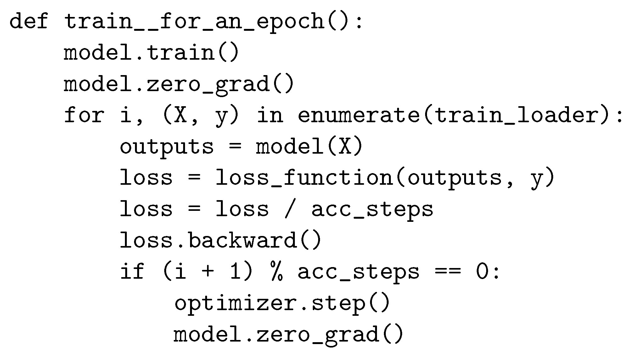
When the desired batch size exceeds the memory capacity of the available GPUs, practitioners often resort to the use of accumulating gradients. That is, instead of having a single forward pass with M examples through the network, number of forward passes are made with examples each. Most of the time, gradients computed using a smaller number of training examples, i.e., , and accumulated over a number of forward passes are identical to those computed using a single forward pass of M training examples. However, it turns out that when BatchNorm is employed in the NN, the gradients can be substantially different for the above two cases. This is a consequence of the mean and variance calculation (see Equation (2)) since each forwarded smaller batch of data will have a different mean and variance than if all M examples were present. Accumulating gradients with BatchNorm can thus be thought as an alternative way of using GhostNorm with the number of forward passes corresponding to the number of groups . A PyTorch implementation of accumulating gradients is shown in the Appendix A, Figure A2.
Finally, the most popular implementation of GhostNorm via BatchNorm, albeit typically unintentional, comes as a consequence of using multiple GPUs. Given GPUs and M training examples, examples are forwarded to each GPU. If the BatchNorm statistics are not synchronized across the GPUs, often the case for image classification, then corresponds to the number of groups .
A practitioner who would like to use GhostNorm should employ the implementation shown in Appendix A. Nevertheless, under the discussed circumstances, one could explore GhostNorm through the use of other means.
2.3.2. Sequential Normalization
The implementation of SeqNorm is straightforward since it applies GroupNorm, a widely implemented normalization technique, and GhostNorm, for which we have discussed three possible implementations, in a sequential manner. A CUDA-native approach is subject to future work.
3. Experiments and Results
In this section, we first strive to take a closer look at the effects of GhostNorm by visualizing the smoothness of the loss landscape during training: a component which has been described as the primary reason behind the effectiveness of BatchNorm. Then, we conduct a number of ablation experiments, comparing both GhostNorm and SeqNorm against other approaches (methods that failed to improve over our baselines are discussed in Appendix D). Finally, we evaluate the effectiveness of both GhostNorm and SeqNorm on the standard image classification data sets of CIFAR-10 (Canadian Institute For Advanced Research), CIFAR-100, and ImageNet. Note that in all of our experiments, the smallest we employ for both SeqNorm and GhostNorm is 4. A ratio of 1 would be undefined for normalization, whereas a ratio of 2 results in large information corruption, i.e., all activations are reduced to either 1 or values.
3.1. Loss Landscape Visualisation
We visualize the loss landscape during optimization on MNIST and CIFAR-10, using an approach that was described by Santurkar et al. [9]. Each time the network parameters are to be updated, we walk toward the gradient direction and compute the loss at multiple points. This enables us to visualize the smoothness of the loss landscape by observing how predictive the computed gradients are. In particular, at each step of updating the network parameters, we compute the loss at a range of learning rates, and store both the minimum and maximum loss. Implementation details are provided in Appendix B.
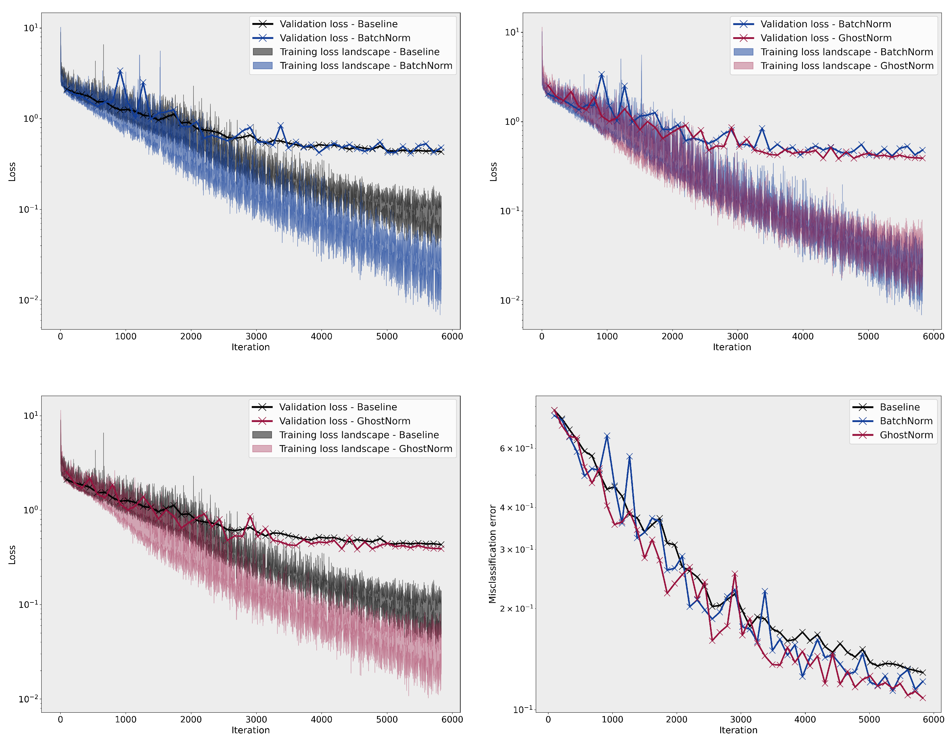
For both data sets and networks, we observe that the smoothness of the loss landscape deteriorates when GhostNorm is employed. In fact for MNIST, as seen in Figure 2, the loss landscape of GhostNorm bears a closer resemblance to our baseline which did not use any normalization technique. For CIFAR-10, as seen in Figure 3, this is only observable toward the last epochs of training. In spite of the above observation, we consistently witness better generalization performance with GhostNorm in almost all of our experiments, even at the extremes, wherein is set to 128, i.e., only 4 samples per group.
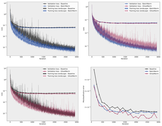
Figure 2.
Comparison of the loss landscape on MNIST between BatchNorm, GhostNorm, and the baseline.
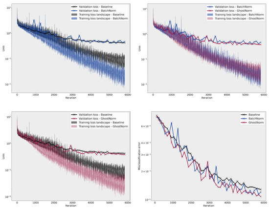
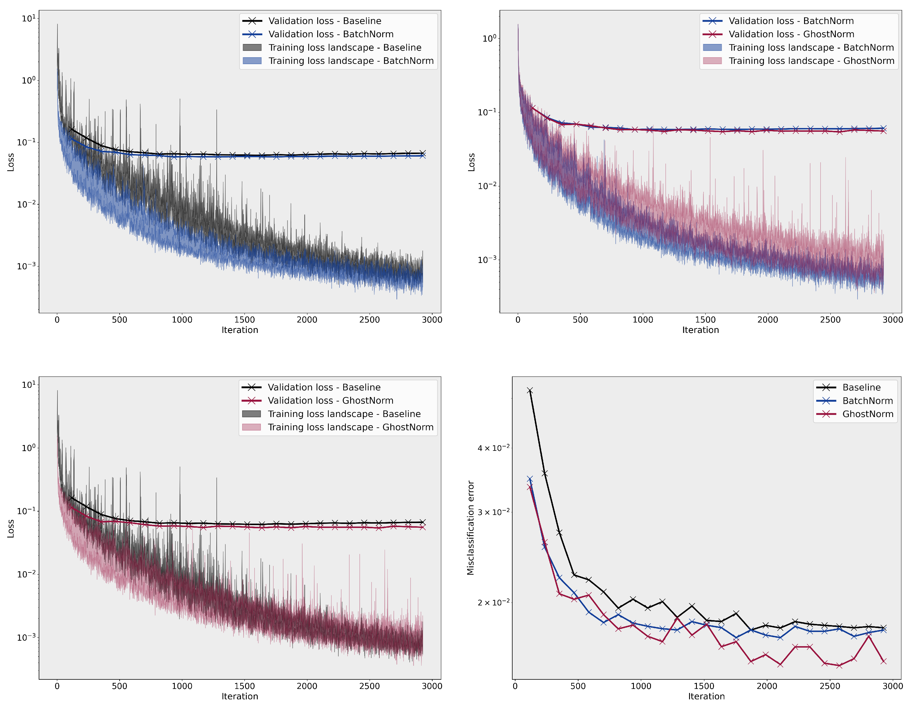
Figure 3.
Comparison of the loss landscape on CIFAR-10 between BatchNorm, GhostNorm, and the baseline.
Our experimental results challenge the often established correlation between a smoother loss landscape and a better generalization performance [9,13]. Although beyond the scope of our work, a theoretical analysis of the implications of GhostNorm when compared to BatchNorm could potentially uncover further insights into the optimization mechanisms of both normalization techniques.
3.2. Image Classification
3.2.1. CIFAR–100
Initially, we turn to CIFAR-100, and tune the hyperparameters of both GhostNorm and SeqNorm in a grid-search fashion. The results are shown in Table 1. We also examine a noisy version of BatchNorm, wherein we inject Gaussian noise on the activations just before normalization. Finally, for all normalization layers, we also train models that employ dropout as well as RandAugment [27]. All of the aforementioned regularization techniques were tuned as described in Appendix C.

Table 1.
Results on CIFAR-100. For SeqNorm, we only show the best results for each . Both validation and testing performance results are averaged over two different runs.
Both GhostNorm and SeqNorm improve upon the BatchNorm baseline by a large margin ( and , respectively). Noisy BatchNorm does not improve the generalization performance, showing that GhostNorm and SeqNorm embed more than just unstructured noise. Models with dropout are omitted since they fail to provide any improvement on the validation set over the baselines. RandAugment substantially improves the BatchNorm () and GhostNorm models (), but fails to benefit models with SeqNorm. Despite the lack of synergy with RandAugment, it is important to note that SeqNorm still manages to surpass the current SOTA performance on CIFAR-100 by [27]. These results support our hypothesis that sequentially applying GhostNorm and GroupNorm layers can have an additive effect on improving NN optimization.
However, the grid-search approach to tuning and of SeqNorm can be rather time consuming (time complexity: ). Hence, we attempt to identify a less demanding hyperparameter tuning approach. The most obvious, and the one we actually adopt for the next experiments, is to sequentially tune and . In particular, we find that first tuning , then selecting the largest for which the network performs well (amongst similarly performing models, select the one with the lowest variance), and finally tuning with to be an effective approach (time complexity: ). In other words, for tuning the hyperparameters of SeqNorm, one first tunes the hyperparameter of GhostNorm , and then the hyperparameter of GroupNorm while keeping constant. Note that by following this approach on CIFAR-100, we still end up with the same best hyperparameter configuration, i.e., and .
3.2.2. CIFAR-10
As the first step, we tune for GhostNorm. We observe that for , the network performs similarly on the validation set at accuracy. We choose for GhostNorm since it exhibits slightly higher accuracy.
Based on the tuning strategy described in the previous section, for SeqNorm, we adopt (lowest variance) and tune for values between 1 and 16, inclusively. Although the network performs similarly at accuracy for , we choose , as it achieves slightly higher accuracy than the rest. Using the above configuration, SeqNorm is able to match the current SOTA on the testing set [28], yet as with CIFAR-100 without the employment of RandAugment.
3.2.3. ImageNet
We first train GhostNorm models with , and find that achieves the best validation accuracy (). SeqNorm with (and ) achieves the best performance () out of values. BatchNorm models only achieve top1 accuracy, lower than GhostNorm, and lower than SeqNorm. Following hyperparameter tuning, the models are trained for more epochs (250 vs. 50) and re-evaluated on the validation set. The difference in performance between the normalization layers is consistent with all the previous results, i.e., the highest is SeqNorm (), then GhostNorm (), and finally BatchNorm ().
In addition to the original ImageNet validation set, we also evaluate our models on three recently released test sets for ImageNet [29]. Without any further retraining (i.e., on the validation set), on average, SeqNorm is able to surpass substantially the reproduced top1 accuracy of BatchNorm, namely by , while GhostNorm also improves the accuracy by . The results for both CIFAR-10 and ImageNet are shown in Table 2.
Table 2.
Results on CIFAR-10 and ImageNet data sets. Both validation and testing performance results of CIFAR-10 are averaged over two different runs. For ImageNet, each model is evaluated on the conventional validation set, as well as on three newly released test sets [29].
4. Discussion
In this work, we first demonstrate the effectiveness of GhostNorm on a number of different networks, learning policies, and data sets. For instance, when using super-convergence on CIFAR-10, GhostNorm performs better than BatchNorm, even though the former normalizes the input activations using 4 samples (i.e., mini-batch is divided into groups of 4 that are normalized based on their group and ), whereas the latter uses all 512 samples. This is antithetical to the common belief that associates poorer estimates of batch statistics, perhaps due to having a smaller sample size, to BatchNorm performance degradation [11,14,20,21]. Instead, our experimental results suggest that grouping along the batch dimensional is effective. Indeed, similar results were observed in GroupNorm, wherein any number of groups would give better results than LayerNorm (all channels in one group) [14]. By providing novel insight on the source of regularization in GhostNorm, and by introducing a number of possible implementations, we hope to inspire further research into GhostNorm and more widespread adoption.
However, we argue that even though GhostNorm and GroupNorm both use grouping, they have vastly different effects on optimization. Based on the understanding developed while investigating GhostNorm, we introduce SeqNorm and follow up with the empirical analysis. Unlike methods such as switchable normalization, we argue that SeqNorm provides a better alternative, since the use of the different normalization techniques is independent of the training optimization [21].
Surprisingly, SeqNorm not only surpasses the performances of BatchNorm and GhostNorm, but even meets or surpasses current SOTA methodologies on CIFAR-10, CIFAR-100, and ImageNet [27,28,29]. The proposed normalization layer results in models that consistently outperform our baseline alternatives with minimal cost (two hyperparameters) yet notable generalization gains. SeqNorm provided performance gains that are comparable, or better, than sophisticated data augmentation strategies [27,28]. Finally, we describe and validate a hyperparameter tuning strategy for SeqNorm that provides a faster alternative to the traditional grid-search approach.
Author Contributions
N.D. conceived the idea of this project. O.A. and N.D. designed and implemented different parts of the methodology, and N.D. conducted the corresponding experiments. The manuscript was written and revised by both authors. O.A. supervised this project. All authors have read and agreed to the published version of the manuscript.
Funding
This research received no external funding.
Institutional Review Board Statement
Not applicable.
Informed Consent Statement
Not applicable.
Data Availability Statement
CIFAR-10 and CIFAR-100 can be found at https://www.cs.toronto.edu/~kriz/cifar.html, accessed on 1 December 2021. ImageNet is available at https://image-net.org/challenges/LSVRC/index.php, accessed on 1 December 2021. The external testing set for ImageNet is available at https://github.com/modestyachts/ImageNetV2, accessed on 1 December 2021.
Acknowledgments
We gratefully acknowledge the support of NVIDIA Corporation with the donation of the Quadro P6000 GPU used for this research. We are also grateful for the support from iCAIRD which is funded by Innovate UK on behalf of UK Research and Innovation (UKRI) (project number: 104690).
Conflicts of Interest
The authors declare no conflict of interest.
Appendix A. GhostNorm Implementations
Herein, we provide both the direct implementation of GhostNorm (Figure A1) as well as through the use of accumulating gradients (Figure A2), as described in Section 2.3.
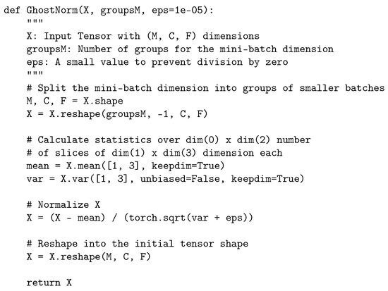
Figure A1.
Python code for GhostNorm in PyTorch.
Figure A1.
Python code for GhostNorm in PyTorch.
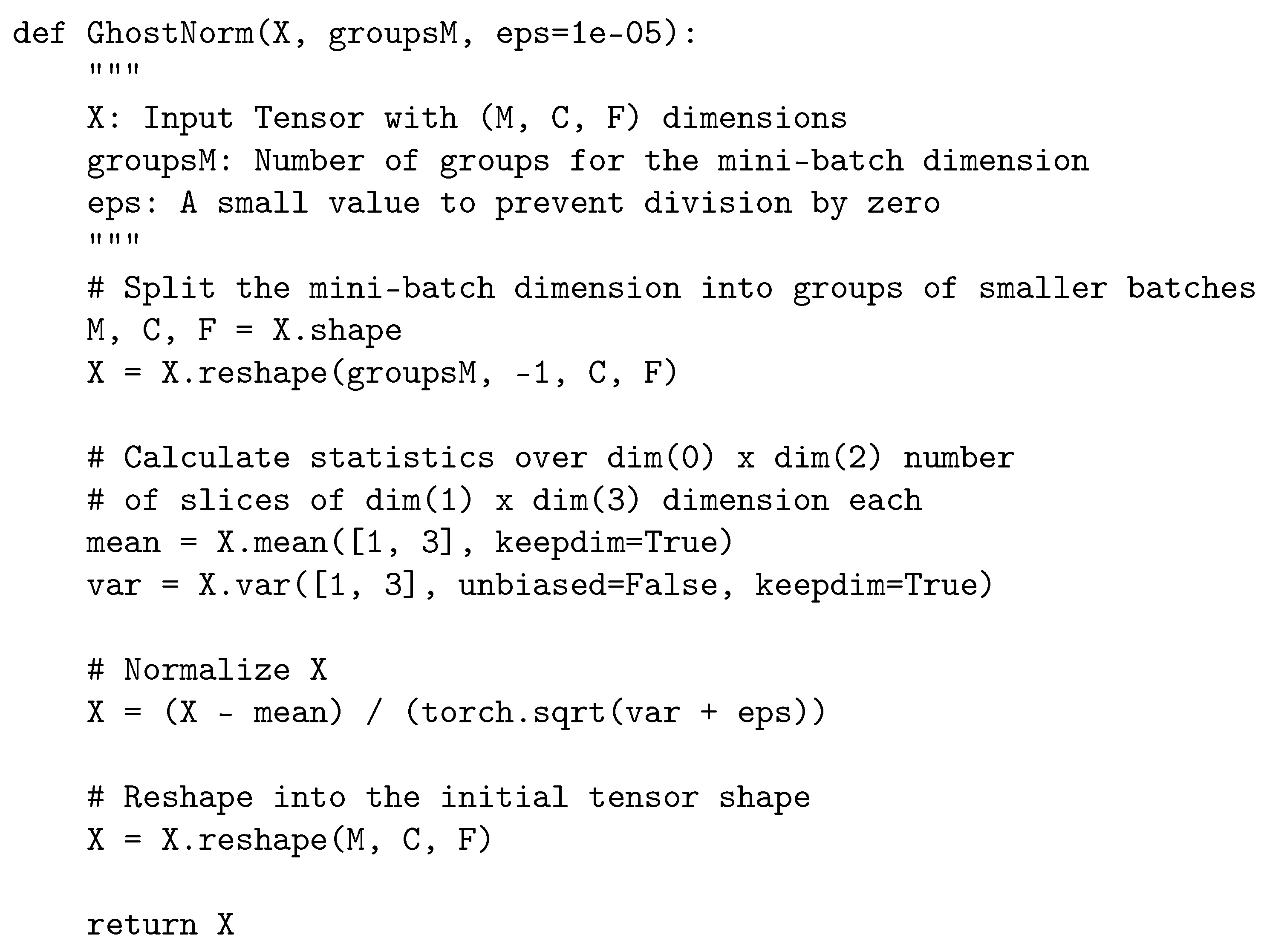
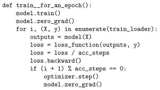
Figure A2.
Python code for accumulating gradients in PyTorch.
Figure A2.
Python code for accumulating gradients in PyTorch.
Appendix B. Loss Landscape Visualization
Appendix B.1. Implementation Details
On MNIST, we train a fully connected neural network (SimpleNet) with two fully connected layers of 512 and 300 neurons. The input images are transformed to one-dimensional vectors of 784 channels, and are normalized based on the mean and variance of the training set. The learning rate is set to for a batch size of 512 on a single GPU.
In addition to training SimpleNet with BatchNorm and GhostNorm, we also train a SimpleNet baseline without any normalization technique.
A residual convolutional network with 56 layers (ResNet–56) [4] is employed for CIFAR-10. We achieve super-convergence by using the one cycle learning policy described in the work of Smith and Topin [30]. Horizontal flipping, and pad-and-crop transformations are used for data augmentation. Most of the hyperparameter values were adopted from the work of Smith and Topin [30]. In particular, we employ stochastic gradient descent with a weight decay of , and a one-cycle learning policy linearly increasing from to in 15 epochs, linearly decreasing to in the next 15 epochs, and decreasing to linearly over the last 10 epochs. The optimizer does not employ any momentum. In order to train ResNet-56 without a normalization technique (baseline), we have to adjust the cyclical learning rate schedule to (, 1).
We train the networks on and training images (CIFAR–10 and MNIST respectively), and evaluate on testing images.
Appendix B.2. Loss Landscape
For MNIST, we compute the loss at 8 learning rates ∈ [, , , , ], whereas for CIFAR–10, we do so for 4 cyclical learning rates ), , , , and analogously for the baseline.
Appendix B.3. Results
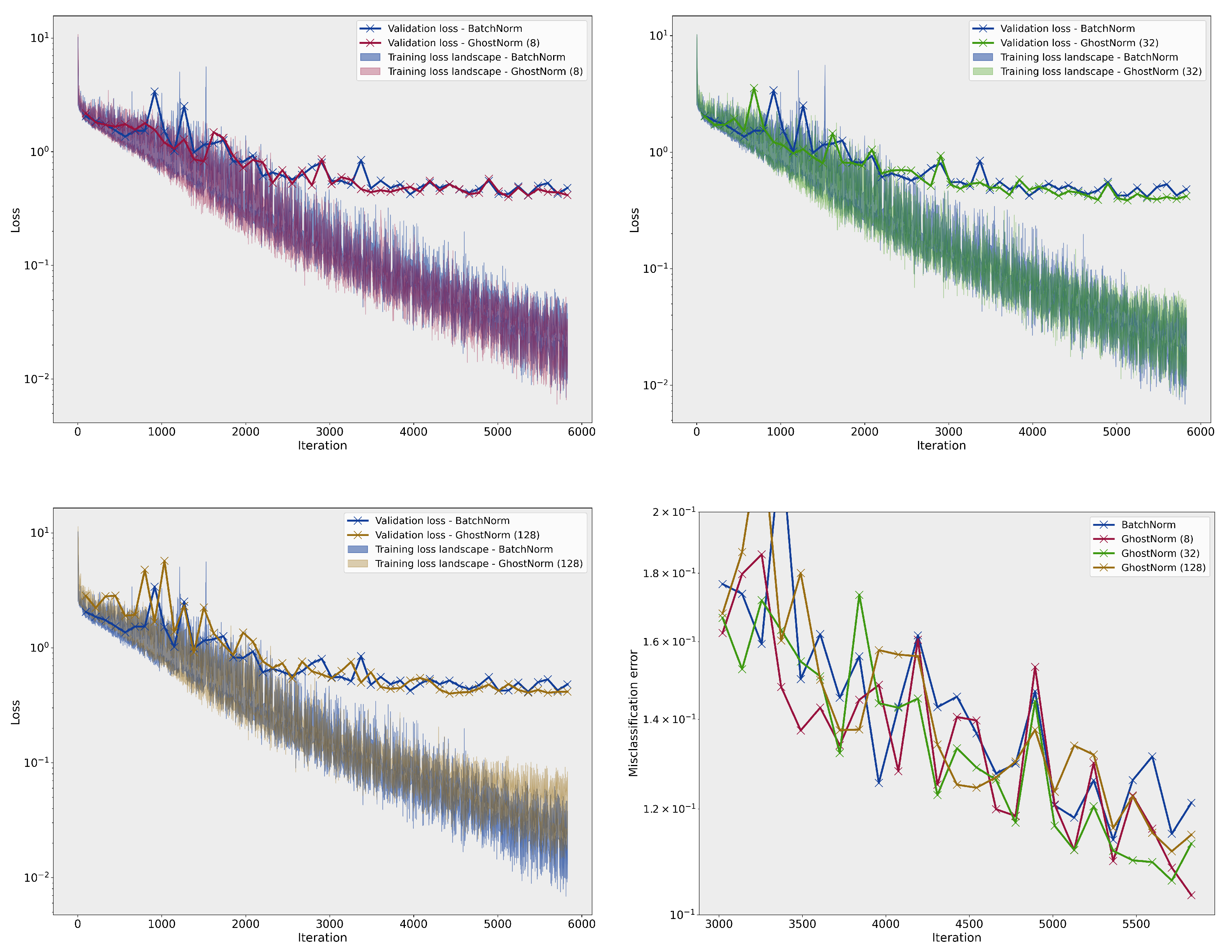
On MNIST, the smoothness of the loss landscape decreases with a larger (see Figure A3). The best model used GhostNorm with set to 64, normalizing over 8 samples. On CIFAR-10, we only observe an effect on the training loss landscape with large values of , (see Figure A4). Nevertheless, all configurations with , i.e., GhostNorm, improved optimization with models performing better than the BatchNorm baseline on the testing set.
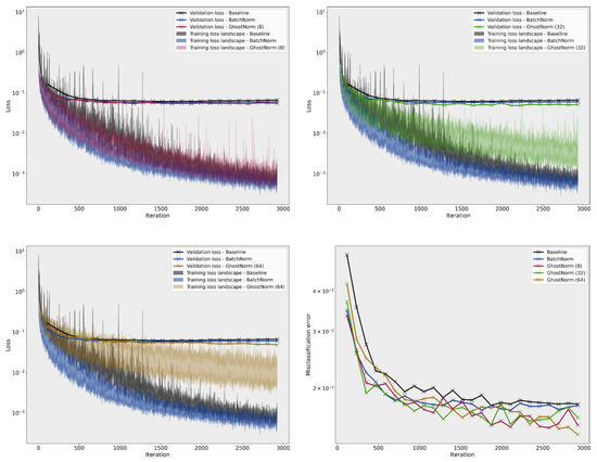
Figure A3.
Comparison of the loss landscape on MNIST between the baseline, BatchNorm, and GhostNorm with different values. The last figure (bottom right) depicts the misclassification error on the testing set during training.
Figure A3.
Comparison of the loss landscape on MNIST between the baseline, BatchNorm, and GhostNorm with different values. The last figure (bottom right) depicts the misclassification error on the testing set during training.
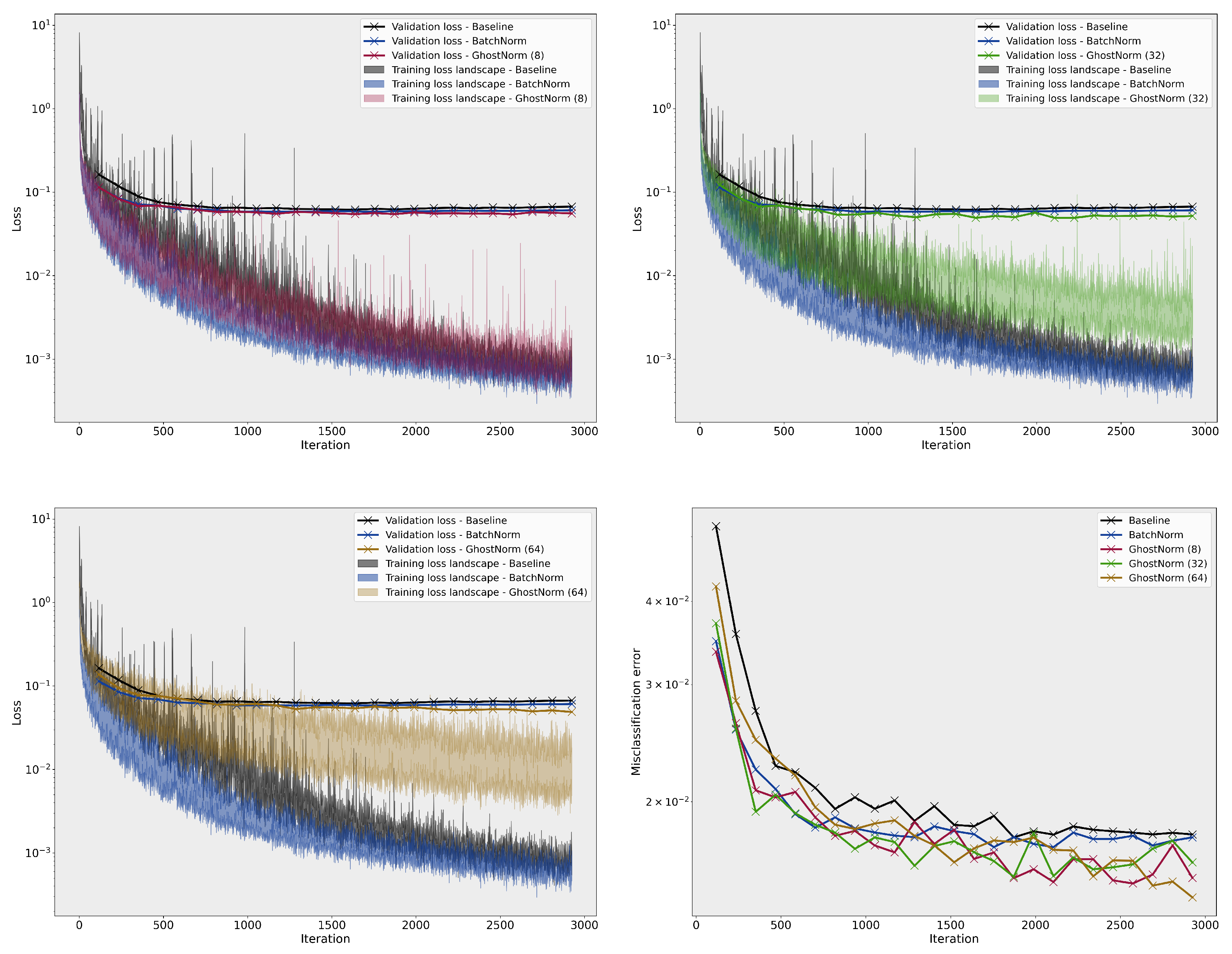
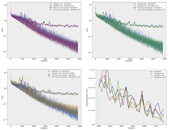
Figure A4.
Comparison of the loss landscape on CIFAR–10 between BatchNorm and GhostNorm with different values. The last figure (bottom right) depicts the misclassification error on the testing set during training.
Figure A4.
Comparison of the loss landscape on CIFAR–10 between BatchNorm and GhostNorm with different values. The last figure (bottom right) depicts the misclassification error on the testing set during training.
Appendix C. Image Classification
Implementation Details
For both CIFAR-10 and CIFAR-100, we employ a training set of images, a validation set of 5000 images (randomly stratified from the training set), and a testing set of . The input data were stochastically augmented with horizontal flips, pad-and-crop and Cutout [31]. We use the same hyperparameter configurations as Cubuk et al. [27]. However, in order to speed up optimization, we increase the batch size from 128 to 512, and apply a warmup scheme [32] that increases the initial learning rate by four times in 5 epochs; thereafter, we use the cosine learning schedule. Based on the above experimental settings, we train Wide-ResNet models of 28 depth and 10 width [33] for 200 epochs. Note that since 8 GPUs are employed, our BatchNorm baselines are equivalent to using GhostNorm with . Nevertheless, to avoid any confusion, we refer to it as BatchNorm. It’s worth mentioning that setting to 8 on 8 GPUs is equivalent to using 64 on 1 GPU.
For ImageNet, we train on 1.28 million training images and evaluate on 50,000 validation images, as well as on three testing sets with 10,000 images each [16]. We adopt the methodology described in the NVIDIA’s public repository for training on 8 GPUs (20.08 docker container) using a ResNet-18 v1.5 architecture. See the repository for the full implementation details. Repository available at https://github.com/NVIDIA/DeepLearningExamples/, accessed on 1 December 2021. We tune our hyperparameters using the 50 epoch script, and then retrain using the 250 epochs script. Both mixed precision (AMP) and DALI are employed. Other than the addition of GhostNorm and SeqNorm, the only other change we implement is to clip the gradients (threshold = 2) as it allows for a more stable training.
For the ablation studies on CIFAR-100, we tune noisy Batch Norm with Gaussian noise of zero mean and standard deviations of , , , …, . The best validation accuracy is achieved with a standard deviation of . For models with dropout, we test values of , , , , and for all BatchNorm, GhostNorm, and SeqNorm. Dropout consistently worsens the validation accuracy and is thus omitted from the results. Finally, for RandAugment, we try N values of and M values of as also reported by Cubuk et al. [27]. The best configurations are as follows: (1, 6) for BatchNorm, (1, 14) for GhostNorm, and (1, 4) for SeqNorm.
Appendix D. Negative Results
A number of other approaches were adopted in conjunction with GhostNorm and SeqNorm. These preliminary experiments on CIFAR-100 did not surpass the BatchNorm baseline performances on the validation sets (most often than not by a large margin), and are therefore not included in detail. Note that given a more elaborate hyperparameter tuning phase, i.e., that would include learning rate, weight decay, these approaches may had otherwise succeeded.
In particular, we experimented with placing GhostNorm and GroupNorm in reverse order for SeqNorm (in retrospect, this could have been expected given what we describe in Section 2.2), and also experimented with augmenting SeqNorm and GhostNorm with weight standardization [13] as well as by computing the variance of batch statistics on the whole input tensor [16]. Finally, on all datasets, we attempted to tune networks with only GroupNorm [14] but the networks were either unable to converge or they achieved worse performance than the BatchNorm baselines.
References
- Ioffe, S.; Szegedy, C. Batch normalization: Accelerating deep network training by reducing internal covariate shift. arXiv 2015, arXiv:1502.03167. [Google Scholar]
- Krizhevsky, A.; Sutskever, I.; Hinton, G.E. ImageNet classification with deep convolutional neural networks. Commun. ACM 2017, 60, 84–90. [Google Scholar] [CrossRef]
- Huang, G.; Liu, Z.; Weinberger, Q.K. Densely Connected Convolutional Networks. arXiv 2016, arXiv:1608.06993. [Google Scholar]
- He, K.; Zhang, X.; Ren, S.; Sun, J. Deep Residual Learning for Image Recognition. In Proceedings of the 2016 IEEE Conference on Computer Vision and Pattern Recognition (CVPR), Las Vegas, NV, USA, 27–30 June 2016; pp. 770–778. [Google Scholar]
- Graves, A.; Mohamed, A.; Hinton, G. Speech recognition with deep recurrent neural networks. arXiv 2013, arXiv:1303.5778. [Google Scholar]
- Sutskever, I.; Vinyals, O.; Le, Q.V. Sequence to Sequence Learning with Neural Networks. In Advances in Neural Information Processing Systems 27; Ghahramani, Z., Welling, M., Cortes, C., Lawrence, N.D., Weinberger, K.Q., Eds.; Curran Associates, Inc.: Red Hook, NY, USA, 2014; pp. 3104–3112. [Google Scholar]
- Silver, D.; Huang, A.; Maddison, C.J.; Guez, A.; Sifre, L.; van den Driessche, G.; Schrittwieser, J.; Antonoglou, I.; Panneershelvam, V.; Lanctot, M.; et al. Mastering the game of Go with deep neural networks and tree search. Nature 2016, 529, 484–489. [Google Scholar] [CrossRef]
- Mnih, V.; Kavukcuoglu, K.; Silver, D.; Rusu, A.A.; Veness, J.; Bellemare, M.G.; Graves, A.; Riedmiller, M.; Fidjeland, A.K.; Ostrovski, G.; et al. Human-level control through deep reinforcement learning. Nature 2015, 518, 529–533. [Google Scholar] [CrossRef]
- Santurkar, S.; Tsipras, D.; Ilyas, A.; Madry, A. How Does Batch Normalization Help Optimization? In Proceedings of the Advances in Neural Information Processing Systems, Montréal, QC, Canada, 3–8 December 2018; Bengio, S., Wallach, H., Larochelle, H., Grauman, K., Cesa-Bianchi, N., Garnett, R., Eds.; Curran Associates, Inc.: Red Hook, NY, USA, 2018; pp. 2483–2493. [Google Scholar]
- Bjorck, N.; Gomes, C.P.; Selman, B.; Weinberger, K.Q. Understanding Batch Normalization. In Advances in Neural Information Processing Systems 31; Bengio, S., Wallach, H., Larochelle, H., Grauman, K., Cesa-Bianchi, N., Garnett, R., Eds.; Curran Associates, Inc.: Red Hook, NY, USA, 2018; pp. 7694–7705. [Google Scholar]
- Ioffe, S. Batch Renormalization: Towards Reducing Minibatch Dependence in Batch-Normalized Models. In Proceedings of the 31st International Conference on Neural Information Processing Systems, Long Beach, CA, USA, 4–9 December 2017; pp. 1942–1950. [Google Scholar]
- Lei Ba, J.; Kiros, J.R.; Hinton, G.E. Layer Normalization. arXiv 2016, arXiv:1607.06450. [Google Scholar]
- Qiao, S.; Wang, H.; Liu, C.; Shen, W.; Yuille, A. Weight Standardization. arXiv 2019, arXiv:1903.10520. [Google Scholar]
- Wu, Y.; He, K. Group Normalization. arXiv 2018, arXiv:1803.08494. [Google Scholar]
- Ulyanov, D.; Vedaldi, A.; Lempitsky, V. Instance Normalization: The Missing Ingredient for Fast Stylization. arXiv 2016, arXiv:1607.08022. [Google Scholar]
- Luo, C.; Zhan, J.; Wang, L.; Gao, W. Extended Batch Normalization. arXiv 2020, arXiv:2003.05569. [Google Scholar]
- Liang, S.; Huang, Z.; Liang, M.; Yang, H. Instance Enhancement Batch Normalization: An Adaptive Regulator of Batch Noise. arXiv 2019, arXiv:1908.04008v2. [Google Scholar] [CrossRef]
- Singh, S.; Shrivastava, A. EvalNorm: Estimating Batch Normalization Statistics for Evaluation. arXiv 2019, arXiv:1904.06031. [Google Scholar]
- Hoffer, E.; Hubara, I.; Soudry, D. Train Longer, Generalize Better: Closing the Generalization Gap in Large Batch Training of Neural Networks. In Proceedings of the 31st International Conference on Neural Information Processing Systems, NIPS’17, Long Beach, CA, USA, 4–9 December 2017; pp. 1729–1739. [Google Scholar]
- Yan, J.; Wan, R.; Zhang, X.; Zhang, W.; Wei, Y.; Sun, J. Towards Stabilizing Batch Statistics in Backward Propagation of Batch Normalization. arXiv 2020, arXiv:2001.06838. [Google Scholar]
- Summers, C.; Dinneen, M.J. Four Things Everyone Should Know to Improve Batch Normalization. arXiv 2020, arXiv:1906.03548. [Google Scholar]
- Wu, J.; Hu, W.; Xiong, H.; Huan, J.; Braverman, V.; Zhu, Z. On the Noisy Gradient Descent that Generalizes as SGD. arXiv 2019, arXiv:1906.07405. [Google Scholar]
- Smith, S.L.; Elsen, E.; De, S. On the Generalization Benefit of Noise in Stochastic Gradient Descent. arXiv 2020, arXiv:2006.15081. [Google Scholar]
- De, S.; Smith, S.L. Batch Normalization Biases Residual Blocks towards the Identity Function in Deep Networks. In Proceedings of the 34th International Conference on Neural Information Processing Systems, NIPS’20, Vancouver, BC, Canada, 6–12 December 2020. [Google Scholar]
- Bronskill, J.; Gordon, J.; Requeima, J.; Nowozin, S.; Turner, R.E. TaskNorm: Rethinking Batch Normalization for Meta-Learning. arXiv 2020, arXiv:2003.03284. [Google Scholar]
- Luo, P.; Ren, J.; Peng, Z.; Zhang, R.; Li, J. Differentiable Learning-to-Normalize via Switchable Normalization. arXiv 2019, arXiv:1806.10779. [Google Scholar]
- Cubuk, E.D.; Zoph, B.; Shlens, J.; Le, Q.V. RandAugment: Practical automated data augmentation with a reduced search space. arXiv 2019, arXiv:1909.13719. [Google Scholar]
- Cubuk, E.D.; Zoph, B.; Mane, D.; Vasudevan, V.; Le, Q.V. AutoAugment: Learning Augmentation Strategies From Data. arXiv 2019, arXiv:1805.09501. [Google Scholar]
- Recht, B.; Roelofs, R.; Schmidt, L.; Shankar, V. Do ImageNet Classifiers Generalize to ImageNet? arXiv 2019, arXiv:1902.10811. [Google Scholar]
- Smith, L.N.; Topin, N. Super-Convergence: Very Fast Training of Neural Networks Using Large Learning Rates. arXiv 2017, arXiv:1708.07120. [Google Scholar]
- DeVries, T.; Taylor, G.W. Improved Regularization of Convolutional Neural Networks with Cutout. arXiv 2017, arXiv:1708.04552. [Google Scholar]
- Goyal, P.; Dollár, P.; Girshick, R.; Noordhuis, P.; Wesolowski, L.; Kyrola, A.; Tulloch, A.; Jia, Y.; He, K. Accurate, Large Minibatch SGD: Training ImageNet in 1 Hour. arXiv 2017, arXiv:1706.02677. [Google Scholar]
- Zagoruyko, S.; Komodakis, N. Wide Residual Networks. arXiv 2017, arXiv:1605.07146. [Google Scholar]

Publisher’s Note: MDPI stays neutral with regard to jurisdictional claims in published maps and institutional affiliations. |
© 2022 by the authors. Licensee MDPI, Basel, Switzerland. This article is an open access article distributed under the terms and conditions of the Creative Commons Attribution (CC BY) license (https://creativecommons.org/licenses/by/4.0/).