Ensemble Convolutional Neural Network Classification for Pancreatic Steatosis Assessment in Biopsy Images

Abstract

Non-alcoholic fatty pancreas disease (NAFPD) is a common and at the same time not extensively examined pathological condition that is significantly associated with obesity, metabolic syndrome, and insulin resistance. These factors can lead to the development of critical pathogens such as type-2 diabetes mellitus (T2DM), atherosclerosis, acute pancreatitis, and pancreatic cancer. Until recently, the diagnosis of NAFPD was based on noninvasive medical imaging methods and visual evaluations of microscopic histological samples. The present study focuses on the quantification of steatosis prevalence in pancreatic biopsy specimens with varying degrees of NAFPD. All quantification results are extracted using a methodology consisting of digital image processing and transfer learning in pretrained convolutional neural networks for the detection of histological fat structures. The proposed method is applied to 20 digitized histological samples, producing an 0.08% mean fat quantification error thanks to an ensemble CNN voting system and 83.3% mean Dice fat segmentation similarity compared to the semi-quantitative estimates of specialist physicians.

1. Introduction

Fat accumulation is a common pathological phenomenon in the pancreas. It is closely related to non-alcoholic fatty pancreas disease (NAFPD), which signals the onset of metabolic syndrome (MetS). Key risk factors for developing NAFPD include obesity, hypertension, and dyslipidemia, which refers to damage to the arteries by blood lipid disorders. This causes the replacement of the acinar cells by steatotic fat droplets, which can significantly contribute to the development of a pro-inflammatory environment causing eventually the progression to type-2 diabetes mellitus (T2DM), severe acute pancreatitis, as well as end-stage cardiovascular disease and pancreatic cancer [1,2].

Published studies from the beginning of this century have shown that histological inflammation, as an extension of NAFPD, is the starting point for the development of further malignancies in which the genetic mechanism has not been fully clarified. This results in incomplete pharmacotherapy, which makes the early diagnosis of pancreatic steatosis a major task. “Pancreatic steatosis” is a commonly used term that is widely characterized by the accumulation of fat droplets in the cytoplasm of cells, thus leading to cellular dysfunction or death [3]. In recent years, it has increasingly become the focus of histopathologists, as there have been also cases where NAFPD patients have blood loss while undergoing pancreatectomy and postoperative pancreatic fistula [1].

Although the pancreas is more prone to the development of steatosis compared to the liver, NAFPD has been less studied than non-alcoholic fatty liver disease (NAFLD). That is because pancreatic biopsy is a strictly responsible invasive procedure for surgeons, which can lead to severe complications for the patient such as hemorrhage and pancreatic fistula, as an abnormal communication between the pancreas and other organs [4]. On the other hand, there are diagnostic limitations to noninvasive medical imaging modalities, such as computed tomography (CT), ultrasonography (US), and magnetic resonance imaging (MRI) when examining pathological and chronic conditions, including fat infiltration and pancreatic cancer. Even though the research community makes an annual effort to make the most of the noninvasive nature of these methods, in recent years and with the development of modern computer vision systems, the microscopic analysis of biopsy images has become the gold standard for diagnosing pathological alterations in the tissue samples. This is because microscopy provides access to all the morphological features of a disease and healthy anatomical structure, which is an element that has significantly reduced the problems of subjective intra-observer and inter-observer interpretations, referring to diagnostic disagreements between physicians.

Confirming the above, there are few pancreatic steatosis quantification studies based on biopsy images, which are mainly based on statistical analyses of semi-quantitative estimates by histopathologists. Starting with the Olsen study [5], his goal was to investigate the degree of lipomatosis in histological pancreatic samples and to determine its association with the age and weight of human donors. The results showed a significant correlation between the three factors as the degree of lipomatosis increased in older and overweight individuals. Wilson et al. [6] attempted to determine the mechanisms of lipid droplets accumulation in histological rat samples. The findings showed that the increased esterification of cholesterol is partly responsible for the formation of adipocytes in the tissue. Nghiem et al. [7] focused on the semi-quantitative evaluation of the fat infiltration between the pancreatic lobules and also its correlation with body mass index (BMI). The high BMI caused increased fat infiltration between the superficial pancreatic lobes as well as the formation of thicker fatty interlobular septa with numerous intralobular fat cells. Mathur et al. [8] determined whether steatosis is a risk factor for postoperative pancreatic fistula. The diagnostics showed that patients with fistula had significantly more intralobular, interlobular, and total pancreatic fat, which were considered to be major risk factors for its occurrence. In a later study [9], the same research team performed tests to determine if fat infiltration and fibrosis accumulation are associated with pancreatic adenocarcinoma individuals. It was observed that patients positive for adenocarcinoma had significantly more pancreatic fat compared to negative patients. As for positive patients, they also showed reduced rates of fibrosis. In the Pinnick et al. work [10], the association of triacylglycerol (TG) with tissue lipid content and T2DM was examined. According to the histological analysis of human biopsies, the quantitative assessment of fat using morphometry was significantly correlated with the TG content and was independent of the diabetic condition of each patient. Rosso et al. [11] examined the association of fat prevalence with the occurrence of pancreatic fistula in patients undergoing pancreaticogastrostomy. The univariate analysis showed that increased pancreatic fat infiltration was associated with the presence of fistula. As in the Olsen study [5], the advanced age and BMI were significantly correlated with increased pancreatic fat levels. Fraulob et al. [12] evaluated the association of NAFPD, fatty liver, and insulin resistance in mouse biopsy specimens. Mice with higher pancreatic and liver fat deposition appeared to be insulin resistant. The authors stated that these phenomena also refer to factors of the human metabolic syndrome, which can eventually lead to chronic pancreatitis. The aim of Gaujoux et al. [13] was to evaluate the effect of BMI in patients who underwent pancreatoduodenectomy as a risk factor for the occurrence of pancreatic fistula. The results showed that pancreatic fat infiltration was more common in patients with high BMI, which are two important prognostic factors for fistula. In contrast, pancreatic fibrosis has not been shown to be a determinant for fistula. As a final for the pancreatic samples study, Van Geenen et al. [14] wanted to identify a possible association between pancreatic steatosis with non-alcoholic fatty liver disease in postmortem human samples. Interlobular and total pancreatic fat were shown to be important prognostic factors for the presence of NAFLD. In addition, the presence of intralobular pancreatic fat was associated with non-alcoholic steatohepatitis (NASH) as opposed to total fat. As previously mentioned, histological examinations of pancreas biopsy specimens are limited to semi-quantitative assessments by physicians. However, in recent years, computational analysis methods have provided effective solutions in the diagnosis of chronic and critical pathogens in biopsy specimens extracted from various organs. In particular, Forlano et. al. [15] applied image processing and machine learning techniques to detect and quantify multiple liver pathogens, including steatosis, hepatocellular ballooning, as well as liver fibrosis and histological inflammation. Guo et al. [16] relied on the Mask R-CNN deep neural network with various ResNet backbone models to automate the segmentation of liver steatotic cells. In recent years, deep learning algorithms have also offered highly efficient automated solutions in the detection and staging of cancer in breast and kidney biopsy specimens. More emphatically, Gandomkar et al. [17] proposed the “MuDeRN” system consisting of multiple deep residual networks combined with a meta-decision tree for the classification of breast cancer subtypes based on a majority of their votes. The breast cancer classification method of Wang et al. [18] was also based on multi-convolutional neural networks. The new framework was applied to cropped image regions, from which convolved feature values were fed into an ensemble support vector machine classifier. Regarding kidney biopsies, Tian et al. [19] applied image processing and machine learning techniques for staging cancer cells according to the four-level Fuhrman grading system. Tabibu et al. [20] employed a hybrid convolutional neural network (CNN) and DAG-SVM classification method to identify three renal cell carcinoma subtypes and separate them from healthy tissue regions. Moreover, research studies based on image processing techniques and machine learning models have been proposed for identifying various intestinal malignancies in biopsy images. Koh et al. [21] developed a multi-stage celiac disease analysis tool employing image preprocessing and machine learning algorithms. Its purpose was to detect and classify areas of villous atrophy based on a modified Marsh grading system. Similarly, Sali et al. [22] proposed a deep learning methodology for automating the celiac disease diagnostic procedure. The deep analysis system utilized a convolutional autoencoder to filter out informative features in image patches extracted from whole slide images. Then, these were inserted in the input layer of deep residual networks to diagnose celiac disease severity using a modified Marsh score. In closing, computer-aided biopsy image analysis has revolutionized the field of histopathology in recent years. Based on this, it is expected that in the future, and with the use of robotic-assisted methods, for minimizing the invasive nature of biopsy extraction, new computational analysis methodologies are to be introduced based on pancreatic microscopy images.

In this work, a methodology for the quantification of fat infiltration in pancreatic biopsy images is presented. The automated analysis is performed on a total of 20 microscopic NAFPD specimens through image segmentation and convolutional neural network classification techniques for the detection of steatosis regions. The general goal is for all fatty areas to be separated from the healthy anatomical structures. As a result of this differentiation, most false-positive fat segmentation results can be minimized, allowing for a more objective fat ratio assessment. This is accomplished by solving a four-class identification problem of four pancreatic tissue alterations, namely: (1) single fat droplet, (2) double-agglomerated fat, (3) multi-agglomerated fat, and (4) tissue artifact. Then, the diagnostic tool’s performance is compared with that derived from semi-quantitative estimates of expert pathologists.

2. Materials and Methods

The following pages describe the method used to quantify the fat ratio in human pancreatic biopsy images. The proposed methodology consists of four main stages in total:

• An image segmentation stage employing image thresholding and morphological filtering techniques in 20 pancreatic biopsy images (with 20× magnification) to extract the tissue area from its background and filter circular white structures.
• Manual annotation of objects of interest in each 20× histological image and calculation of the semi-quantitative degree of steatosis by clinicians. At the same time, export of annotated objects in the form of image patches for applying transfer learning in four pretrained convolutional neural networks (CNNs).
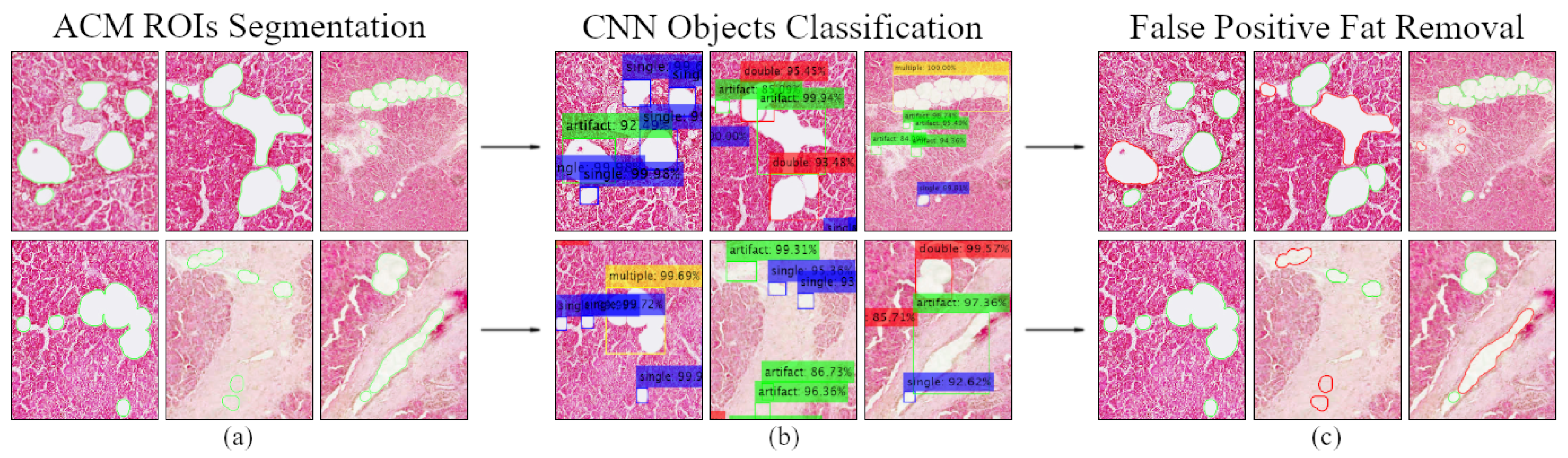
• Classification of the segmented regions of interest in step 1 based on the majority of trained CNN models’ votes and eliminating most false-positive fat segmentation results.
• Calculation of the fat ratio for each 20× biopsy image and evaluation of the automated diagnostic method by determining its deviation from the semi-quantitative estimates of doctors.

Figure 1 shows a flowchart of the proposed diagnostic system, including the image preprocessing and CNN classification steps, used for the quantification of pancreatic steatosis prevalence in NAFPD patients.

2.1. Histological Image Dataset

The proposed methodology is tested on 20 pancreatic biopsy samples coming with varying degrees of NAFPD steatosis from the University of Oxford (Oxford, UK). They are surgical samples of normal donor pancreases taken at the time of transplantation. All the extracted tissue samples are histologically colored with the hematoxylin and eosin (H&E) stain, which has become the gold standard in histopathological diagnosis in recent years. After the tissue coloring and biopsy slide preparation procedures, all pancreatic specimens are scanned at 20× magnification.

2.2. Image Processing and Segmentation Stage

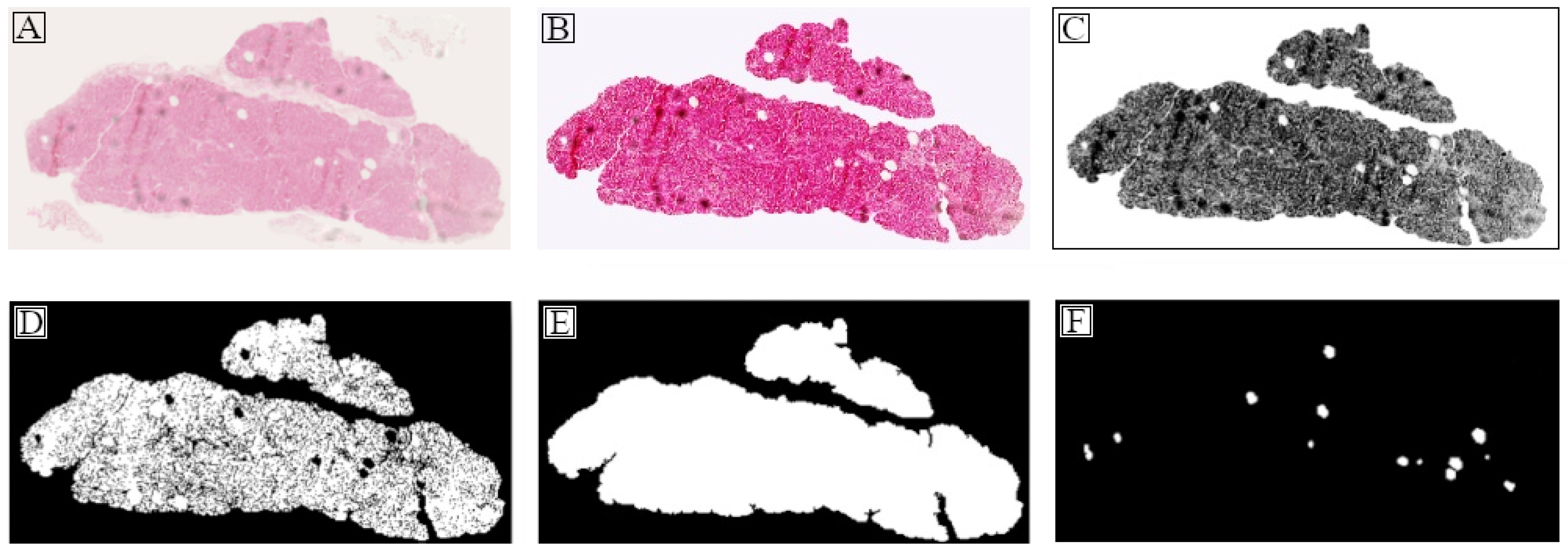
2.2.1. Tissue Region Extraction

Each scanned biopsy is loaded to the image analysis method as a three-dimensional array consisting of 8-bit integer values in each RGB color channel (Figure 2A). Initially, it is preferred to apply histogram equalization to all channels of the RGB sample to adjust the image intensities and enhance the contrast. This preserves all the histogram-based image information on all three color channels. Subsequently, the background noise is reduced by computing the area for each 8-connected pixel region, which consists of objects with neighboring pixels linked in a horizontal, vertical, or diagonal direction. Then, connected pixel regions with an area less than 0.3% of the largest region are discarded as part of the pancreatic sample (Figure 2B). Following the contrast enhancement and image denoising steps, a large part of the biopsy reflects a bright background, whereas the H&E histological sample includes bright red and purple pixels.

For the histological region to be extracted from its white background, the color image is first converted to a corresponding two-dimensional grayscale, with saturation applied to the lower 1% and upper 1% of all pixel values. This improves the vividness of the gray pixel intensities (Figure 2C) and allows the image processing method to accurately determine the outer boundaries of the tissue area. In the next step, the adaptive thresholding algorithm based on the local mean intensity, as the selected first-order statistic, is applied to the neighborhood of each grayscale pixel. This technique emerged as the best option for this problem to be solved, as the dataset consists of 20 biopsy images with significant changes in their pixel intensities. In other words, it can calculate a different threshold value for each pixel in the image, allowing greater tolerance to the intensity changes between the tissue regions. This is achieved by calculating the integral image, which allows multiple overlapping rectangular windows to determine the average intensity value for each pixel neighborhood [23]. More specifically, for each term to the left-top of each (x, y) pixel coordinate, a function f(x, y) is applied to convert the pixel intensity values to real numbers for the integral image I(x, y) to be computed with:

$$I(x,y)=f(x,y)+I(x-1,y)+I(x,y-1)-I(x-1,y-1)$$

(1)

Then, for any rectangle in the integral image with an upper-left corner (x₁, y₁) and a lower-right corner (x₂, y₂), the sum of the function f is calculated with:

$$\sum _{x=x_1}^{x_2}\sum _{y=y_1}^{y_2}f(x,y)=I(x_2,y_2)-I(x_2,y_1-1)-I(x_1-1,y_2)+I(x_1-1,y_1-1)$$

(2)

After the algorithm’s convergence, a threshold is set in the pixels of the integral image by applying a sensitivity value within the closed interval [0, 1], where a higher sensitivity value equals a larger number of pixels added to the foreground (tissue area). On the contrary, an excessively high sensitivity value can have a negative effect, as part of the background pixels may be included in the foreground. With this in mind, the sensitivity value is set to 0.599, after some trial and error. As a final step, this separation of pixels leads to the conversion of the grayscale image to binary, where (a) black pixels (logical ‘0’) → background and (b) white pixels (logical ‘1’) → tissue (Figure 2D).

According to Figure 2D, the adaptive thresholding approach has included several black regions within the histological area as background pixels. This is a common occurrence in histological images because they often contain many healthy anatomical structures or low-contrast tissue pixels. For these areas to be connected and for the histological sample to be accurately determined, a hole filling function is used to remove all black objects and replace them with logical ‘1’ values (Figure 2E).

2.2.2. Objects of Interest Segmentation

Currently, the main focus of the image preprocessing method is to filter circular white objects pointing to potential fat cells inside the previously segmented tissue area. This process takes place in the binary image of Figure 2D, where all the necessary morphological elements have been retained and can lead to the segmentation of the steatosis structures in the original RGB biopsy image. At first, the binary values are reversed, resulting in all black circular objects within the tissue region being highlighted in white. Afterward, by initializing a circular mask with an 8-pixel radius, a repeating loop is applied performing morphological opening on the circular white structures with an increasing radius of 2 pixels in each iteration. When the radius of the structuring element reaches a maximum of 36 pixels, the loop terminates. These numbers are chosen because physicians believe that tissue objects outside this radius range are artifacts that indicate the presence of various healthy anatomies. The main feature here is that any binary pixels that do not completely intersect the structural element are removed from the binary image and the external boundaries of each filtered white object are smoothed at the same time. Finally, active contour models are called upon to converge at the outer boundaries of every filtered circular white structure in the new morphological image shown in Figure 2F.

Upon completion of the morphological processing, the segmentation of circular objects takes place in the original RGB biopsy image and green color for each active contour. The segmentation of circular structures results appears to be sufficient, as the active contour models have converged to the boundaries of all histological objects of interest. However, several false-positive fat droplets were observed by the authors, which are in fact artifacts involving either tissue areas with low-contrast values or circular veins, convex sinusoids, and ducts. In this case, the inclusion of false-positive fat findings leads to an overestimation of the pancreatic steatosis prevalence in each microscopic sample, which has a negative impact on the identification of each patient’s pathological condition. To overcome this diagnostic obstacle, the next phases of the methodology use an ensemble classification system based on the training of convolutional neural networks (CNNs), so that false-positive steatosis structures are excluded from fat ratio calculations.

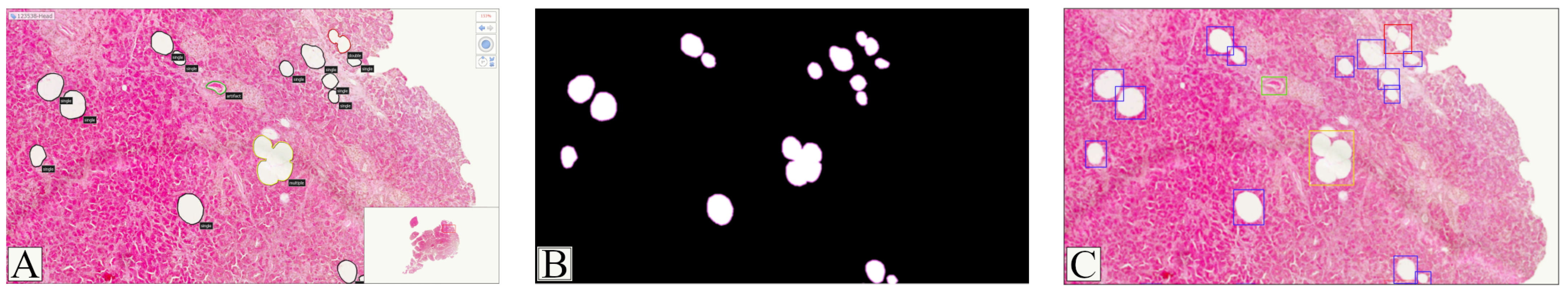
2.3. Histological Images Annotation

Given the current success of deep learning algorithms in image classification tasks, forming a multi-CNN system to solve the diagnostic problem in the previous image segmentation stage is preferred. Since we are dealing with a supervised learning system for classification purposes, clinicians were called to decide on the class labels that define the most frequently occurring tissue anatomies in the 20 NAFPD biopsy samples. Particularly, the anatomical structures in the pancreatic samples were evaluated by two histopathologists. During the evaluation process, the tissue findings agreed upon by the experts were included in the digital form of the annotation. Following that, the specialists observed cases of objects with a similar circular shape with a single fat droplet, but containing red blood cells, eventually being characterized as veins. Furthermore, the phenomenon of adjacent fat cells agglomeration was noted, especially in individuals with an increased pancreatic steatosis ratio. As a result, their edges merge, forming structures with morphological features (e.g., size, extent, eccentricity) comparable to healthy histological objects such as the sinusoids and pancreatic ducts. Based on these findings, four histological class objects are manually annotated for semi-quantitative and automated diagnostic purposes: (1) single fat droplet, (2) double-agglomerated fat region, (3) multiple-agglomerated fat region, and (4) tissue artifact (Figure 3A). The first three classes encompass all types of fat accumulation in the NAFPD tissue, whereas the histological artifact class includes all healthy structures that must be excluded when calculating the patient’s steatosis ratio.

2.3.1. Semi-Quantitative Steatosis Evaluation

Two steps are performed so that the reliability of the developed diagnostic tool’s performance can be later determined. First, the semi-quantitative steatosis ratio is calculated for each biopsy specimen by dividing the total area of annotated pixels forming either single, double-agglomerated, or multiple-agglomerated fat objects by the total area of the segmented histological region (Figure 2E). Ultimately, a binary image is produced, which is later used as the ground-truth steatosis image (Figure 3B) and helps in calculating the automated diagnostic tool’s fat segmentation similarity with the doctors’ estimates.

2.3.2. Exporting Training Data from Manual Annotations

The manual annotation procedure is performed with the NDP.view2 (Hamamatsu Photonics, Hamamatsu, Japan) histopathological tool. Figure 3A shows its environment, thanks to which the objects of interest are marked with a freehand tool and with a different color per histological class. Then, the 2D Cartesian coordinates of each annotated sample, showing its position in the H&E biopsy image, are automatically recorded in an XML file. In addition, for each tissue object, a class label is assigned by the doctors: (1) “single” (black contour), (2) “double” (red contour), (3) “multiple” (yellow contour), and (4) “artifact” (green contour).

After all the biopsy images (n = 20) are annotated, a method is called for reading their 2D coordinates, which leads to the calculation of their bounding box. This enables all regions of interest to be extracted as image patches from the 20× whole slide images (WSIs) for CNN model training. Before extracting them, the x-axis, y-axis, width, and height (x, y, w, h) coordinates for each computed bounding box are rounded to the nearest integer and then increased by 5 pixels to expand its size (Figure 3C). This is preferred because the bounding box converges to an object’s boundaries, removing edges that might provide informative features during the CNN training process. Finally, using a crop tool, the parameterized image patches are extracted and stored in folders according to their class label.

2.4. Data Preprocessing and Deep Learning

2.4.1. Image Augmentation and Class Balancing

After completing the image patches extraction process, the final count reveals an unbalanced dataset with (a) 2400 single, (b) 342 double, (c) 335 multiple, and (d) 870 artifact samples, a common obstacle in supervised learning methodologies that can lead to reduced classification performance. To balance the dataset, first all image patches in the majority class “single” are reduced to 1320 randomly chosen samples. That is because there is no significant difference in the schematic and textural properties between the single fat droplets and therefore their number is reduced. Instead, those in the “double”, “multiple” and “artifact” minority classes are subjected to image augmentation techniques to increase their number. Horizontal (x-axis) image flipping, vertical (y-axis) image flipping, and horizontal in combination with vertical flipping are all examples of these augmentation techniques. In further detail,

Table 1. Image patches augmentation techniques for class balancing.

Class Label	Initial Count	Removed Images	Image Augmentation	Augmented Count	Final Count
single	2400	1080	-	-	1320
double	342	-	• horizontal flip (x-axis) • vertical flip (y-axis) • horizontal + vertical flip	1026	1368
multiple	335	-	• horizontal flip (x-axis) • vertical flip (y-axis) • horizontal + vertical flip	1005	1340
artifact	870	-	• horizontal + vertical flip	870	1740

Balanced dataset split steps: 1: Gather all the image patches resulting from the “Final Count” column (n = 5768). 2: Form a training subset consisting of 4080 randomly selected augmented and non-augmented “single”, “double”, “multiple”, and “artifact” samples (1020 per class). 3: Form a validation subset consisting of 800 random non-augmented samples (200 per class). 4: Form a testing subset consisting of 400 random non-augmented samples (100 per class). 5. Discard the remaining 488 image patches.

shows the applied augmentation techniques to the minority class samples, as well as the steps for splitting the balanced dataset into training, validation, and testing subsets.

The aforementioned class balancing techniques yield 5280 anatomical specimens (1320 for each pancreatic class), a sufficient number for applying transfer learning to pretrained CNN models. This new dataset is then split into (a) 4080 training, (b) 800 validation and (c) 400 testing samples. According to the balanced dataset separation process in Table 1, it is noted that the validation and testing subsets include non-augmented samples, as is commonly suggested, whereas the training subset consists of a mixture of non-augmented and augmented image patches.

2.4.2. Transfer Learning in Pretrained CNN Models

Transfer learning techniques have emerged as a reliable method for adapting pretrained convolutional neural networks to new object recognition problems in recent years. For this work, an ensemble CNN classification method of pancreatic fat structures is formed using a combination of shallower and deeper CNN topologies for the steatosis ratio to be calculated in NAFPD biopsy specimens. These refer to the (a) AlexNet [24], (b) VGG-16 [25], (c) VGG-19 [25], and (d) ResNet-50 [26] architectures that are loaded along with their pretrained weights from the ImageNet dataset.

After loading the aforementioned CNNs, the number of their training parameters is calculated to determine whether to freeze weights on their initial layers or not. Rounding these numbers to the nearest integer showed that the AlexNet model consists of 61 million trainable parameters, while VGG-16 consists of 138, VGG-19 consists of 144, and ResNet-50 consists of 25.6 million. These findings are in agreement with the numbers reported in the [24,25,26] papers. According to these numbers, there is a considerable discrepancy between AlexNet and ResNet-50 with VGG-16 and VGG-19, with the latter two being regarded as “very deep” neural networks. As a result, it is decided that all weights in the first two convolutional blocks of VGG-16 and VGG-19 are to be frozen. In general, when applying transfer learning to much deeper models, the weight-freezing approach in their initial layers is recommended, since they have generalized to most low-level features (e.g., edges, shapes), and updating them may result in overfitting the new histopathological data.

The training of the four CNN networks is performed once on a single NVIDIA RTX 2070 Super GPU and shares the following common training parameters: (a) a maximum of 10 training epochs, (b) a mini-batch size of 32 image patches, (c) a global learning rate of 0.0001, a preferred value in transfer learning tasks ensuring that each fine-tuned model does not deviate significantly from the corresponding original, (d) a validation patience number equal to 3, in case a CNN presents the same validation accuracy value three times during training, and (d) the SGDM optimizer used in the backpropagation method. Last but not least, the “model checkpoint” option has been enabled to save the weights that produce the highest validation accuracy at the end of each training epoch.

While considering further transfer learning techniques, the “weight learn rate factor” and “bias learn rate factor” parameters are taken into consideration in the last fully connected layer of each CNN architecture. Here, the 1000 neurons indicating the number of classes in the ImageNet dataset have been reduced to 4, allowing each deep model to adapt to the new object recognition problem. Each parameter is expressed as a non-negative scalar multiplied by the global learning rate, such that the neurons of the parameterized fully connected layer can generalize faster to the new pancreatic structures classification task. Specifically, the two parameters for the AlexNet and ResNet-50 networks are set to 10 (10 × (1 × 10${}^{-4}$) = 0.001), whereas in the deeper VGG-16 and VGG-19, they are equal to 20 (20 × (1 × 10${}^{-4}$) = 0.002).

Having completed the final fully-connected layer and weight-freezing configurations, the number of new trainable parameters is recalculated for each CNN topology.

Table 2. Applied parameters for transfer learning to pretrained CNN models.

CNN Model	Trainable Parameters (Initial)	Frozen Weights	Trainable Parameters (Final)	Weight Learn Rate Factor	Bias Learn Rate Factor
AlexNet	60,965,224	-	56,868,224	10	10
VGG-16	138,357,544	• conv. block 1 • conv. block 2	134,260,544	20	20
VGG-19	143,667,240	• conv. block 1 • conv. block 2	139,570,240	20	20
ResNet-50	25,583,592	-	23,534,592	10	10

shows the training options per pretrained network as well as the differences between the initial and final trainable parameters, which result in a decrease of up to 4 million parameters.

2.4.3. Classification of Tissue Objects and Fat Ratio Calculation

After transfer learning, each CNN model is asked to make predictions on the testing subset (Section 2.4.1) so that its classification performance in unknown pancreatic specimens can be assessed. Each image patch of the balanced data set is scaled according to the required size at the input layer of each pretrained neural network using the bicubic interpolation method. The identification of histological structures as well as the extraction of statistical measurements from the classification report (

Table 3. Comparison of classification testing results.

CNN Model	Mean Performance Metrics (%)
	Accuracy	Precision/PPV	Sensitivity/Recall	F1-Score	Specificity/TNR	NPV	ROC AUC	PRC AUC
AlexNet	97.25	97.25	97.25	97.25	99.08	99.08	99.87	74.64
VGG-16	97	97.08	97	97.04	99	99.01	99.86	74.59
VGG-19	95.25	95.37	95.25	95.31	98.42	98.43	99.83	74.50
ResNet-50	94.25	94.37	94.25	94.31	98.08	98.11	99.58	73.80
Ensemble CNN	98.25	98.25	98.25	98.25	99.42	99.42	99.73	99.47

) is performed initially on each CNN network. Then, the majority of prediction votes for each pancreatic structure, based on the individual model characterizations, are taken into account in an ensemble CNN approach. The maximum softmax probabilities, indicating how confident each CNN is in its predictions, are also used to determine the majority pancreatic class in the ensemble classification system, which is analyzed in Algorithm 1 below.

Having measured the deep models’ classification capability in the testing data, their aim now is to characterize the unknown circular objects from the Section 2.2.2 and to reduce the number of false-positive fat findings. Similar to the procedure in Section 2.3.2, each ACM-segmented structure is exported as an image patch and fed as input to each CNN architecture. Later, its histological class is also determined by the ensemble CNN voting method. At the end of the classification process, the area of the predicted fat pixels is calculated and divided by the corresponding one of the segmented histological regions (Section 2.2.1). The produced result indicates the ratio of pancreatic fat filtration in every 20× microscopy image. Lastly, the diagnostic error is retrieved for each biopsy sample, which refers to its deviation from the semi-quantitative steatosis evaluations by specialist physicians.

Algorithm 1 Ensemble CNN System

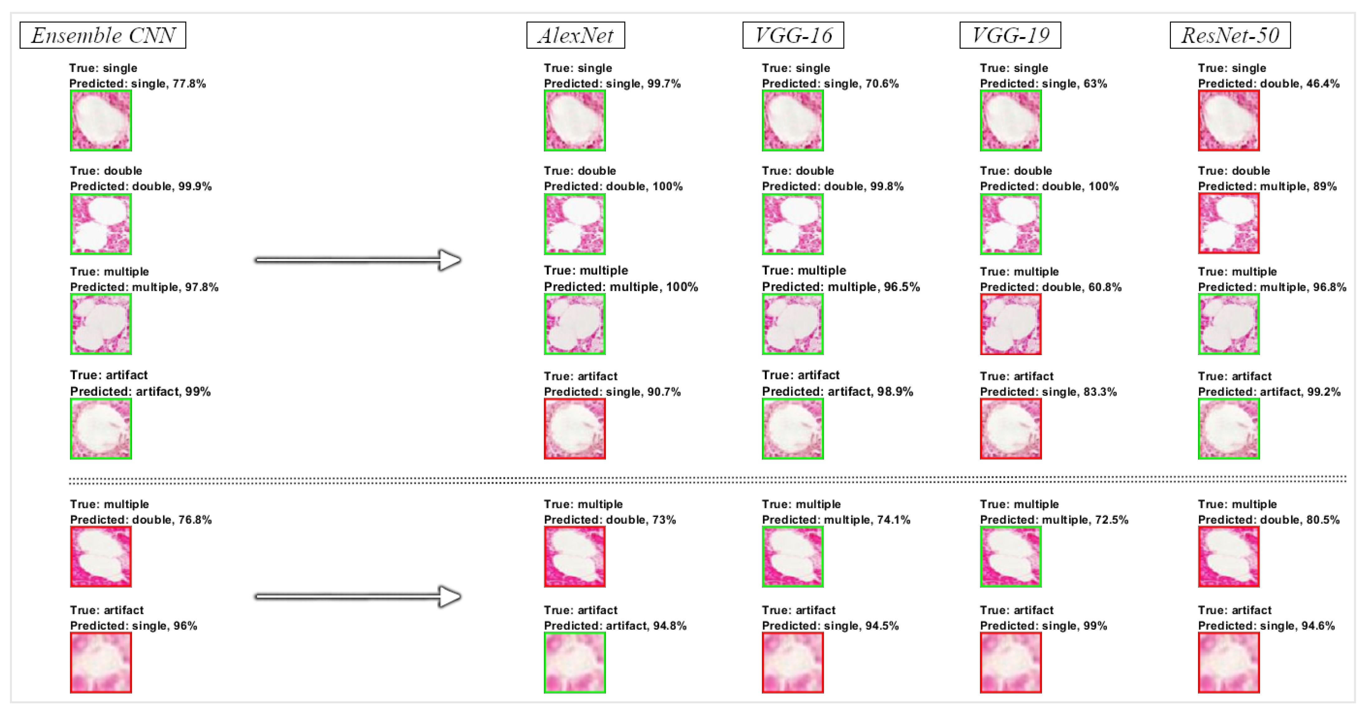
1: Begin Data Preprocessing 2:    Load the 20× biopsy image and its ACM-segmented objects 3:    Calculate and increase each ACM object’s bounding box by 5 pixels 4:    Crop the image patches and determine their number $\left(N_I\right)$ 5:    Specify the number of deep CNNs $\left(N_D\right)$ and predicted images $\left(N_P\right)$ 6: End 7: Begin Ensemble CNN Classification 8:    For $i=1,\dots ,N_I$ do 9:     For $j=1,\dots ,N_D$ do 10:      Determine the [i, j] class label 11:      Retrieve the [i, j] prediction probability 12:    End 13:   End 14:   For $k=1,\dots ,N_P$ do 15:    Filter the most frequent predicted class label 16:    If there are 4 different predicted classes do 17:      Retrieve the maximum prediction probability 18:      Retrieve its corresponding class label 19:    Else If there are 2 different predicted classes do 20:      Calculate the 1st $\left(M{P}_1\right)$ and 2nd $\left(M{P}_2\right)$ mean probabilities 21:      Keep the max mean probability and its corresponding class 22:      If $M{P}_1$ equal to $M{P}_2$ do 23:        Keep one mean probability with a random state 24:        Retrieve its corresponding class label 25:      End 26:    Else do 27:      Retrieve the majority of votes class label 28:      Calculate its mean class probability 29:    End 30:   End 31: End

3. Results

In this section, the classification performance in the testing data, as well as the visualization of the most informative features that contribute to the discrimination of the four examined tissue alterations in the 20× biopsy images are analyzed. Next, the steatosis quantification results coming from two stages are presented: (1) the segmentation of circular objects, referring to potential fat cells prior to their characterization, and (2) the exclusion of false-positive fat findings via the CNN classification step. At the same time, the absolute error produced by these two approaches is compared in all NAFPD histological samples (n = 20). Thereafter, fat detection results employing the ensemble CNN classification system are displayed as well as its fat segmentation similarity with steatotic regions manually annotated by histopathologists.

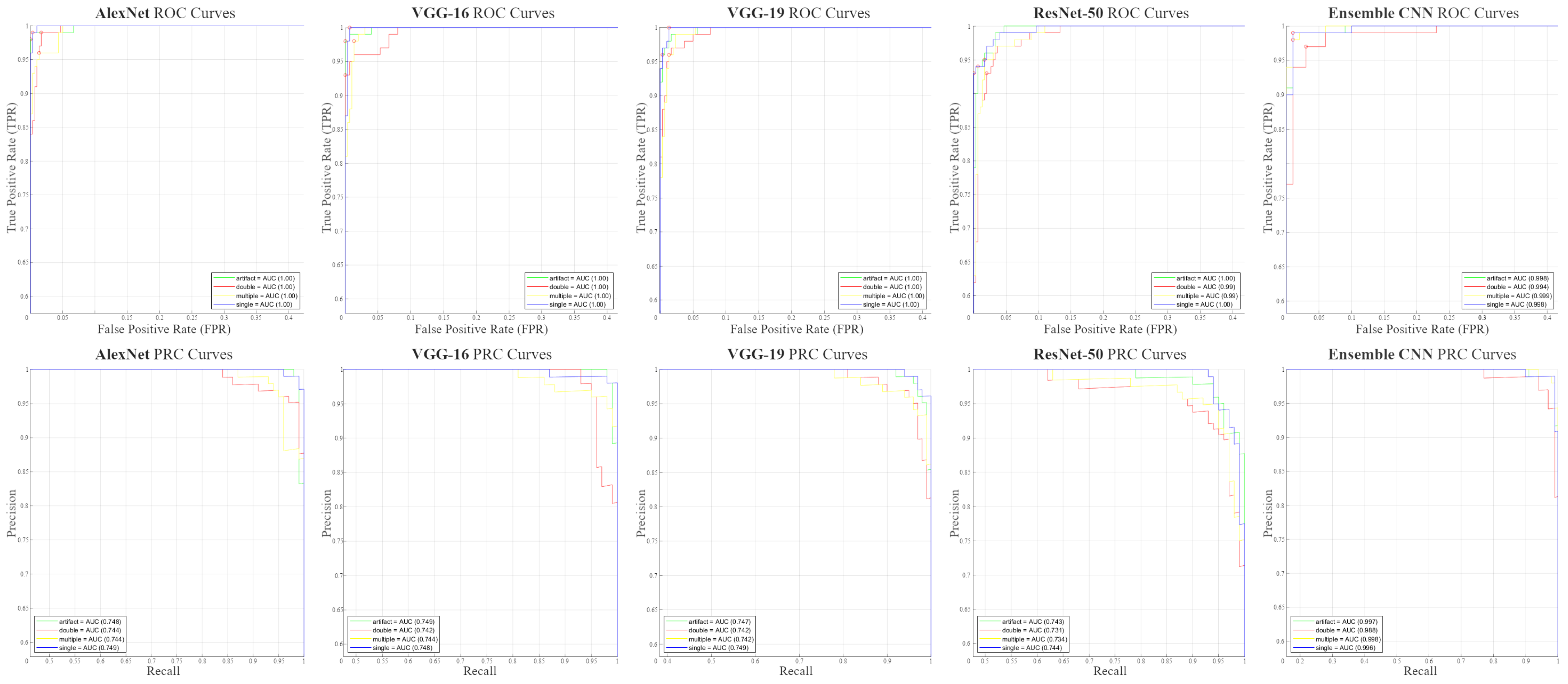
3.1. Testing Performance Measurements

Following the previous section, certain statistics from the classification report in the testing subset (Section 2.4.1) are exported to validate the best CNN classifier (Table 3). These refer to the accuracy, precision/positive predictive value (PPV), sensitivity/recall, specificity/true negative rate (TNR), F1-score, negative predictive value (NPV), ROC-AUC, and PRC-AUC. The ensemble CNN method emerges as the most optimal with accuracy: 98.25%, F1-score: 98.25% and specificity: 99.42%, AlexNet comes in second (accuracy: 97.25%, F1-score: 97.25%, specificity: 99.08%), VGG-16 in third (accuracy: 97%, F1-score: 97.04%, specificity: 99%), VGG-19 in fourth (accuracy: 95.25%, F1-score: 95.31%, specificity: 99.42%), and ResNet-50 in fifth (accuracy: 94.25%, F1-score: 94.31%, specificity: 99.08%).

Concerning the validation accuracy during transfer learning, this equals 95.88% for the AlexNet model, which is produced with the optimal weights from the 9th training epoch (out of 10), thanks to the “model checkpoint” option. The corresponding for VGG-16 is 96.88% with the optimal weights of the 4th epoch. With the final weights of the 10th epoch, on the other hand, the validation accuracy is equal to 95.63% for VGG-19 and 92.13% for ResNet-50. In the ensemble voting system, the value is equal to 97%, which is the highest validation performance.

Then, the thresholds for plotting the ROC and PRC curves are calculated for each of the four pancreatic classes (Figure 4), along with the estimated ROC-AUC and PRC-AUC values. In addition, in the ROC curves, the optimal operating points are indicated by a red circle. For each class, the optimal point is determined by moving a straight line with a slope value S from the upper-left corner of the ROC plot (FPR = 0, TPR = 1) down and to the right, until it intersects its ROC curve. They are referred to as optimal, since in their position, they can identify most of their class samples correctly [27]. It must be noted that the ensemble CNN algorithm takes into account only the maximum softmax probability of each fine-tuned model’s class prediction. Therefore, the remaining three classes’ probabilities cannot be used to calculate the ROC and PRC thresholds. To address this issue, the 4-class threshold calculation problem is divided into four binary problems using the One-vs-Rest (OvR) strategy [28]. It is recalled that for each tissue sample $x_i\subseteq X$ in the testing subset, a prediction label $y_i\in$ {single, double, multiple, artifact} is retrieved using four individual CNN classifiers with $f_k$ for $k\in$ {AlexNet, VGG-16, VGG-19, ResNet-50}. Following that, the mean maximum prediction probability determined in Algorithm 1 is used to calculate the majority of class votes for each testing sample:

$$\widehat{y}=\overline{\underset{k\in \{1\dots 4\}}{argmax}}{f}_k\left(X\right)$$

(3)

where from the $\widehat{y}$ predictions, four new label vectors are constructed with the class names in each of them being: (1) “single”–“nonsingle”, (2) “double”–“nondouble”, (3) “multiple”–“nonmultiple”, and (4) “artifact”–“nonartifact”. In addition, the absolute difference between the mean prediction probability and 1 (the highest possible in the softmax [0, 1] confidence interval) is calculated for each binary label opposite to that of the classification.

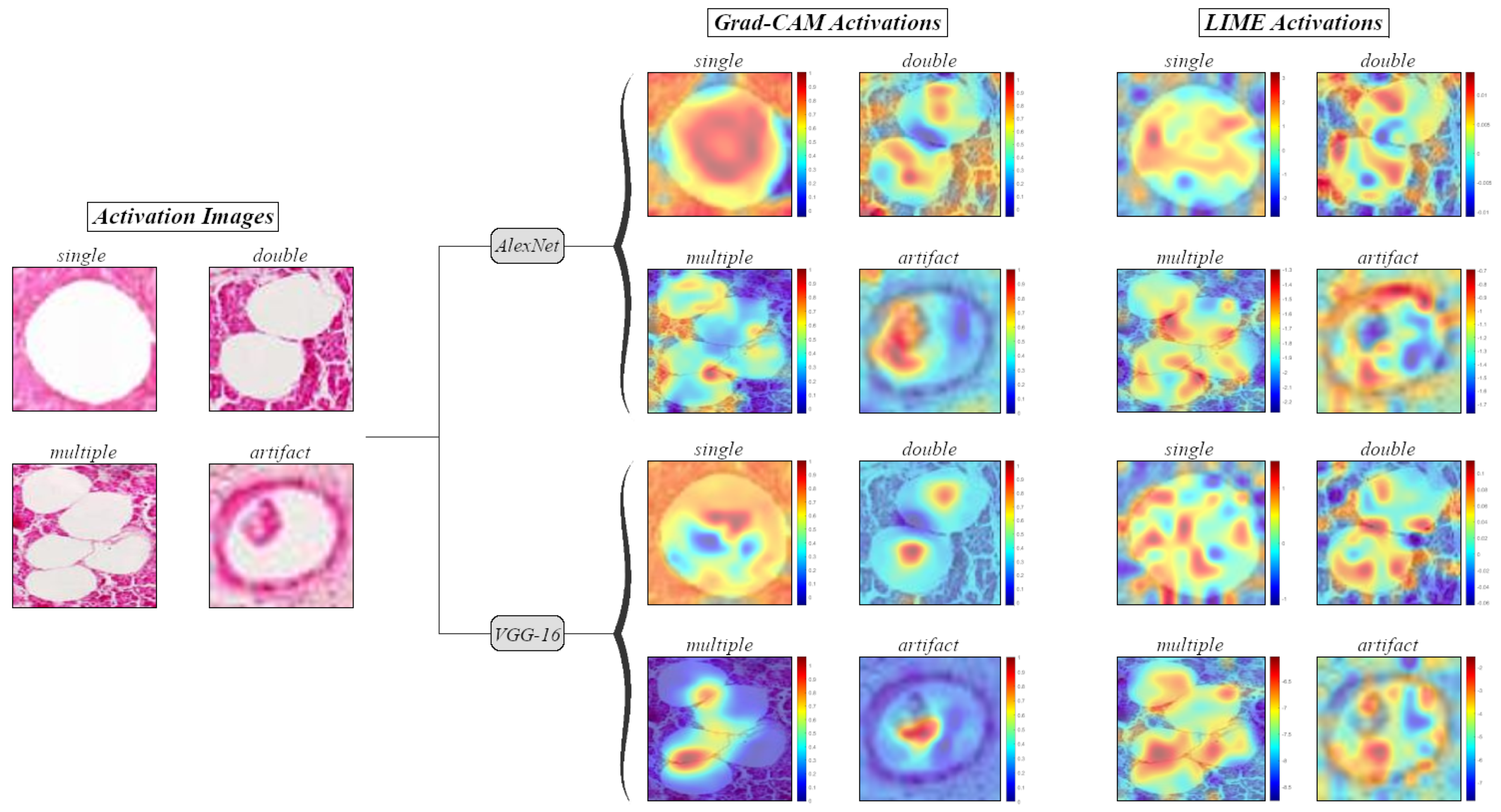
3.2. Visualization of Informative Features

The Grad-CAM (gradient-weighted class activation mapping) and LIME (local interpretable model-agnostic explanations) activation methods are applied to four image patches, one for each histological class, to highlight the most informative microscopic features when classifying a healthy or disease microscopic structure (Figure 5). The processes are performed on the most optimal AlexNet and VGG-16 networks, according to the classification report in Table 3. The Grad-CAM activations are computed by taking into account the gradient of the classification score with respect to convolutional features of a specific layer in the two deep networks [29]. Here, the ReLU activations of the last AlexNet (“relu5”) convolutional layer and VGG-16 (“relu5_3”) convolutional block are declared as the required feature maps with non-singleton spatial dimensions.

The LIME activations [30] are retrieved by fitting a linear regression model with Lasso regularization to 100 filtered features from all AlexNet and VGG-16 layers. This number produces a grid of 10 × 10 square features based on the aspect ratio of each synthetic LIME image (n = 3072). Then, the generated LIME maps are upsampled using the bicubic interpolation method to match the spatial resolution of each image patch, which is equivalent to the size of the input layers in the AlexNet (227 × 227) and VGG-16 (224 × 224) networks. In the end, by combining the LIME feature maps with the Grad-CAM technique, the most informative regions of the four pancreatic structures appear as a smooth heatmap. Both Grad-CAM and LIME heatmap visualizations are performed with an alpha data transparency value of 0.5 in the original image patches.

3.3. Pancreatic Steatosis Quantification Results

At first, the focus is on

Table 4. Pancreatic fat quantification results.

Testing Image (20×)		Fat Ratio (%) Image Segmentation (FSegm)	Fat Ratio(%) Regions Classification (FClass)					Fat Ratio (%) Manual Annotations (FDoc)
		FACM	FAlexNet	FVGG-16	FVGG-19	FResNet-50	FEnsembleCNN	FAnnot
1	120216-Head	1.83	1.72	1.63	1.70	1.59	1.66	1.74
2	120216-Tail	1.58	1.37	1.21	1.32	1.30	1.29	1.31
3	120485-Tail	1.89	1.71	1.59	1.65	1.65	1.66	1.77
4	120495-Body	2.56	1.71	1.44	1.48	1.40	1.48	1.63
5	120495-Head	1.88	1.64	1.55	1.57	1.57	1.62	1.79
6	121543-Body	5.75	5.11	4.82	4.86	4.88	4.92	5.08
7	121543-Head	6.54	6.12	5.76	5.89	5.89	6.00	5.99
8	122020-Body	0.70	0.39	0.28	0.39	0.32	0.36	0.24
9	122020-Head	1.15	0.59	0.39	0.53	0.43	0.53	0.41
10	122020-Tail	1.22	0.61	0.45	0.50	0.48	0.47	0.44
11	122088-Body	0.52	0.40	0.35	0.36	0.33	0.35	0.36
12	122088-Tail	1.47	0.79	0.63	0.73	0.68	0.71	0.63
13	122288-Body	3.22	1.82	0.97	1.07	1.26	1.07	0.99
14	122288-Tail	0.68	0.41	0.34	0.42	0.36	0.39	0.35
15	122662-Body	1.38	0.16	0.08	0.11	0.09	0.10	0.05
16	122662-Tail	1.05	0.30	0.25	0.30	0.25	0.28	0.25
17	123538-Head	3.04	2.52	2.40	2.50	2.50	2.47	2.55
18	123883-Tail	2.84	2.62	2.41	2.52	2.33	2.56	2.39
19	123948-Tail	1.84	1.57	1.42	1.51	1.41	1.50	1.44
20	HP-0937	2.41	2.10	2.05	2.10	2.10	2.08	2.14
Mean Value:		2.18	1.68	1.50	1.58	1.54	1.58	1.58
StD:		1.57	1.55	1.49	1.50	1.51	1.53	1.57

, which shows the fat quantification rates for each 20× pancreatic image. The percentages come from the circular objects segmentation method (column 2), their characterization by the four pancreatic objects classification method (column 3), and the physicians’ semi-quantitative estimates using the NDP.view2 annotation tool (column 4). It is recalled that during the classification stage, the quantifications are performed with the help of individual pretrained CNN topologies in which learning transfer is applied as well as by an ensemble CNN classifier (Algorithm 1).

As can be seen in Table 4, the classification stage ($F_{Class}$) yields lower mean steatosis rates than the image segmentation method ($F_{Segm}$). More emphatically, the mean rates generated from the CNN classifications vary from 1.50% to 1.68%, which is a value range less than 2.18% of the image segmentation stage. The lower mean values relate to the fact that most false-positive fat structures are classified as tissue artifacts and thus are excluded from the steatosis ratio quantifications. Therefore, fat infiltration areas with a “single”, “double”, or “multiple” class label are only included in the fat prevalence calculations.

In column 4 of Table 4, the semi-quantitative assessments of physicians ($F_{Doc}$) for each pancreatic sample are included, which leads to

Table 5. Pancreatic fat quantification error.

Testing Image (20×)		Classification Error (%) from Annotations (Cerr)					Image Segmentation Error (%) from Annotations (Serr)
		AlexNeterr	VGG-16err	VGG-19err	ResNet-50err	EnsembleCNNerr	ACMerr
1	120216-Head	0.02	0.11	0.04	0.15	0.08	0.09
2	120216-Tail	0.06	0.10	0.01	0.02	0.02	0.26
3	120485-Tail	0.06	0.18	0.12	0.12	0.11	0.13
4	120495-Body	0.08	0.19	0.15	0.22	0.14	0.93
5	120495-Head	0.16	0.24	0.23	0.22	0.18	0.09
6	121543-Body	0.03	0.26	0.21	0.20	0.16	0.67
7	121543-Head	0.13	0.23	0.10	0.10	0.00	0.54
8	122020-Body	0.15	0.04	0.15	0.07	0.12	0.46
9	122020-Head	0.18	0.02	0.12	0.02	0.12	0.74
10	122020-Tail	0.17	0.01	0.07	0.04	0.03	0.78
11	122088-Body	0.04	0.01	0.00	0.03	0.01	0.16
12	122088-Tail	0.15	0.01	0.10	0.05	0.08	0.84
13	122288-Body	0.83	0.02	0.08	0.27	0.08	2.22
14	122288-Tail	0.06	0.01	0.06	0.01	0.04	0.33
15	122662-Body	0.11	0.03	0.07	0.04	0.05	1.33
16	122662-Tail	0.05	0.01	0.05	0.00	0.04	0.80
17	123538-Head	0.03	0.15	0.05	0.05	0.09	0.49
18	123883-Tail	0.23	0.02	0.13	0.06	0.17	0.45
19	123948-Tail	0.13	0.02	0.07	0.04	0.05	0.39
20	HP-0937	0.05	0.09	0.04	0.04	0.06	0.27
Mean Value:		0.14	0.09	0.09	0.09	0.08	0.60
StD:		0.17	0.09	0.06	0.08	0.05	0.50

showing the absolute error values for the circular structures filtering stage ($S_{err}$) and their classification as fat findings ($C_{err}$). Here, the ensemble CNN algorithm has the minimum mean absolute error of 0.08% in comparison to the second most efficient VGG-16 (0.0879%), as well as the ResNet-50 (0.0880%), VGG-19 (0.0927%), and AlexNet (0.14%) models. In 19 of the 20 total biopsy specimens, the classification stage produces a lower diagnostic error than the image segmentation method before the characterization of unknown histological structures, which presents a mean 0.6% value. The only non-optimal performance is found in sample no. 5 (“120495-Head”) with fat prevalence rates in all five classifiers being less than 1.88% of the image processing stage, according to Table 4. This shows an underestimation of the fat ratio during the classification step, as “artifact” class labels have been assigned to true-positive agglomerated or non-agglomerated fat regions. In conclusion, the standard deviation of the ensemble CNN absolute errors equals 0.05%, which is the smallest value compared to the corresponding ones produced by the individual CNN networks (0.06% to 0.17%) and the image segmentation method (0.5%), indicating a more balanced diagnostic performance in applying its voting method.

We now turn to the visualization of the fat detection method in sections of various histological images. The visualization takes place first in Figure 6a, which shows the image preprocessing stage’s segmentation result of candidate fat structures. It should be noted again that the presence of low-contrast color sections in the image has resulted in the inclusion of healthy histological sections as fat droplets. Furthermore, the presence of adjacent circular objects has led to the merging of their outer boundaries, leading to the segmentation of healthy histological anatomies other than agglomerated fat regions. For these incorrect inclusions to be removed from the quantitative fat estimates, the bounding box is determined for each unknown ACM-segmented object and then classified with the ensemble CNN method (Figure 6b). In most cases, single lipid droplets, double-agglomerated, and multiple-agglomerated fat regions are successfully distinguished from histological artifacts with high probability values (85–100%). Eventually, most false-positive fat findings are excluded from the quantification of the degree of steatosis in Figure 6c.

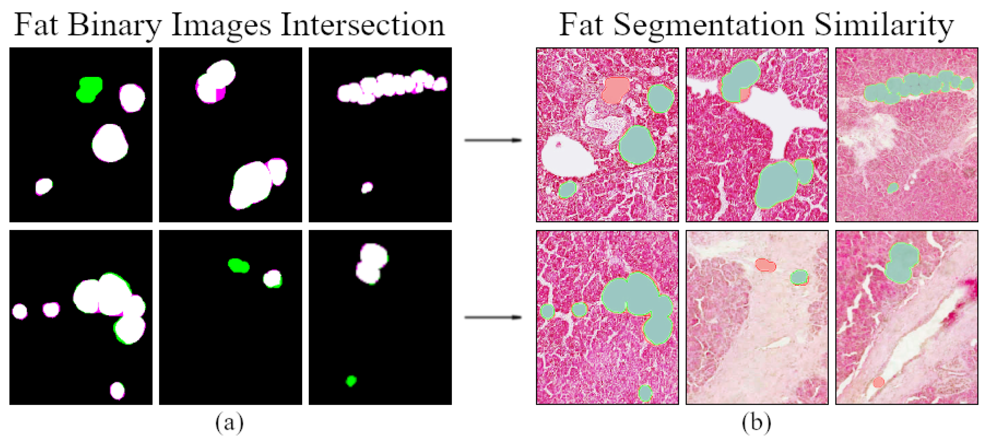
3.4. Fat Regions Segmentation Similarity

After assessing the fat ratio prevalence and computing the absolute diagnostic error for each pancreatic biopsy, the next step focuses on another technique for measuring the reliability of the proposed methodology. This relates to the calculation of fat segmentation similarity between two binary images: (1) the ground truth image derived from the manual fat region annotations and (2) the fat detection method with the employed CNN architectures. The comparison is made with the Sorensen–Dice similarity coefficient [31], which is obtained using the formula below:

$$D_{coeff}(GT,SG)=\frac{2\left(\right|GT\cap SG\left|\right)}{\left|GT\right|+\left|SG\right|}$$

(4)

where the |GT| and |SG| sets denote the ground truth and computed segmentation binary images, respectively, and ‘∩’ denotes the intersection points of logical ‘1’ values in their 2D pixel grid. The preceding Equation (4) can also be expressed in terms of true-positive (TP), false-positive (FP), and false-negative (FN) number of pixels [32].

$$D_{coeff}(GT,SG)=\frac{2TP}{2TP+FP+FN}$$

(5)

Based on Equation (5), the intersection result of ground truth and computed segmentation images is shown in Figure 7a. More specifically, three different pixel shades are visible: (1) white pixels referring to the intersection of logical ‘1’ values between the two binary images, as true-positive fat regions, (2) green pixels indicating false-positive fat region inclusions from the ensemble CNN system, and (3) false-negative magenta pixels indicating unsuccessful fat inclusions from the image preprocessing and CNN classification stages. The final segmentation similarity results are displayed in the original H&E biopsy sections (Figure 7b). These visualizations are produced by applying the logical AND (nonzero elements at that same image coordinates) and XOR (nonzero elements at separate image coordinates) operators to the two binary images specified above. Here, the successfully segmented fat pixels are indicated with a green overlay, whereas the incorrect ones are indicated with red. This representation helps in the analysis of the final fat segmentations in Figure 6c, where a further distinction can be made between correctly and incorrectly included pathological alterations in the steatosis ratio quantitative evaluations.

From the above,

Table 6. Sorensen–Dice fat segmentation similarity.

Testing Image (20×)		AlexNetDice	VGG-16Dice	VGG-19Dice	ResNet-50Dice	EnsembleCNNDice
1	120216-Head	91.8	90.3	91.6	91.7	91.0
2	120216-Tail	88.0	91.0	89.1	90.0	90.3
3	120485-Tail	87.7	86.4	86.5	86.2	87.0
4	120495-Body	78.1	82.4	80.5	82.3	82.3
5	120495-Head	87.0	87.5	86.4	87.0	88.5
6	121543-Body	89.0	90.1	89.5	89.8	90.2
7	121543-Head	90.5	91.7	91.2	90.7	90.9
8	122020-Body	60.2	66.0	60.5	64.9	63.4
9	122020-Head	70.0	76.9	73.1	66.4	73.3
10	122020-Tail	71.6	80.7	77.5	77.4	79.9
11	122088-Body	81.9	83.0	86.1	84.1	85.9
12	122088-Tail	78.9	83.4	82.5	80.9	81.9
13	122288-Body	63.1	84.2	80.5	77.4	83.6
14	122288-Tail	79.9	86.9	79.7	79.0	81.3
15	122662-Body	36.2	57.8	47.7	54.6	53.1
16	122662-Tail	82.7	86.8	82.9	80.0	85.4
17	123538-Head	90.6	92.5	91.6	89.0	91.6
18	123883-Tail	87.7	89.8	89.5	83.6	88.2
19	123948-Tail	84.4	88.4	87.0	85.6	87.0
20	HP-0937	91.0	91.8	88.4	91.3	91.3
Mean Value:		79.5	84.4	82.1	81.6	83.3
StD:		13.76	8.82	11.00	9.81	9.90

presents the Dice segmentation similarity coefficients for each fatty image. The coefficients are derived from the fat detection approach using the individual CNN and ensemble CNN algorithms. The research team’s objective was to acquire scores of at least 70% for the ensemble classification approach as the cut-off value, indicating a very good level of agreement between the computational diagnoses and the visual–manual evaluations of clinicians.

From Table 6 it can be said that there is a very good Dice agreement in 18 of 20 NAFPD images. $EnsembleCN{N}_{Dice}$ similarities with coefficients below 70% are found in samples no. 8 (“122020-Body”) and no. 15 (“122662-Body”). The lower target scores are related to the low-fat percentages for the two samples, according to the physicians’ estimations in Table 4 (122020-Body = 0.24% and 122662-Body = 0.05%). In particular, due to the small number of fat structures, every unsuccessful pixel intersection between the ground truth and computed segmentation images significantly diminishes the similarity coefficient. Nevertheless, all five CNN models have mean Dice scores of above 70%, leading the ensemble CNN method to come in second (83.3%) after the optimal VGG-16 network (84.4%), revealing a weakness in its voting system in a few cases. In closing, VGG-19 has the third-best mean performance (82.1%), ResNet-50 has the fourth-best (81.6%), and AlexNet has the lowest (79.5%).

4. Discussion

Non-alcoholic fatty pancreas disease (NAFPD) is the most prevalent pathological condition in individuals with increased body mass index (BMI) and advanced age (>50 years). Steatosis, which refers to fat infiltration in the pancreatic tissue, is a symptom of NAFPD and is responsible for pancreatic cell hyperplasia, insulin resistance, $\beta$-cell dysfunction, and type-2 diabetes mellitus (T2DM) [33]. To an advanced degree, NAFPD can progress to non-alcoholic steatopancreatitis (NASP), indicating chronic inflammation and histological fibrosis and eventually pancreatic cancer [34]. These two conditions have aroused the interest of physicians for their early diagnosis and follow-up in recent years.

This paper aims to solve the problem of steatosis prevalence quantification in pancreatic biopsy specimens with a methodology employing image segmentation and deep neural network classification techniques. Specifically, an image dataset is extracted from manual annotations and used for transfer learning to pretrained convolutional neural network (CNN) topologies. Then, the fine-tuned CNNs are asked to distinguish between healthy histological artifacts and fat accumulation areas, which are classified as single fat droplets, double-agglomerated, or multiple-agglomerated fat regions. Finally, a voting system in an ensemble CNN classification approach takes into account all individual CNN model characterizations for the majority class of each segmented microscopic object to be determined. The multi-CNN classification system yields a 0.08% mean steatosis quantification error and 83.3% mean Dice fat segmentation similarity in 20 pancreatic biopsy images (carrying a 20× magnification).

It should be remembered that the ensemble CNN classification capability for the 400 testing samples (Section 3.1) is analyzed before the identification of any unknown segmented structure in Section 2.2.2. The ensemble CNN approach employing the voting strategy in Algorithm 1 is called upon to determine the majority class of each tissue object by taking into account its predicted label $y\in$ {single, double, multiple, artifact} and the corresponding softmax probability from the individual AlexNet, VGG-16, VGG-19, and ResNet-50 architectures. Figure 8 shows that the voting method has made four correct classifications (green borders) and two incorrect ones (red borders). In most situations, the softmax probabilities from the individual CNNs are thought to be the main cause for including the incorrect pancreatic class. In future studies, for the classification and the disease quantification errors to be reduced, weights will be assigned to the prediction probabilities based on statistics from the classification report (Table 3) as well as new ones before determining the majority classes, allowing the decision of the most optimal CNNs to be taken into account more than the less generalized ones.

According to

Table 7. Time complexity versus performance per CNN architecture.

CNN Model	Time Complexity		Performance (%)
	Training (min)	Testing (s)	Testing Accuracy	Fat Ratio Error (Mean)	Fat Ratio Error (StD)
AlexNet	1.38	0.5	97.25	0.14	0.17
VGG-16	11.07	2.1	97	0.0879	0.09
VGG-19	13.56	2.3	95.25	0.0927	0.06
ResNet-50	9.58	1.9	94.25	0.088	0.08
Ensemble CNN	35.59	15.1	98.25	0.08	0.05

, there are some confusing results about the performance of each single model. It could be reported that strict classification metrics (such as Accuracy, Precision, Recall, etc.) measure the ability of the models to characterize each fat item (single, double, or multiple); however, the medical question involves and requires the effective estimation of fat’s expansion in the tissue, which is computed via the fat ratio error. Under this consideration, Table 7 shows that although AlexNet performs better in classification accuracy than VGG-16 and VGG-19 performs better than ResNet-50, they present a higher fat ratio error. The latter indicates that probably AlexNet and VGG-19 fail to efficiently characterize some large multiple fat droplets, which significantly affects the fat ratio estimation. Furthermore, it could be also reported that according to the total time complexity of the ensemble model, the computation effort is affordable, making the employment of the proposed voting system meaningful, combined with its effectiveness and efficiency.

Even so, the improved results in relation to the segmentation stage of unknown objects justify the inclusion of supervised models for the elimination of histological artifacts in the fat quantification process. In addition, the decision to differentiate all fat accumulation regions (single, double, and multiple) with different class labels proved to be correct, particularly in terms of preventing fat agglomeration areas from being misclassified as histological artifacts with similar morphological features. Moreover, it appears that the inclusion of background pixels in the image patches can provide valuable edge and schematic properties to the deep classifiers. This advantage, together with the deep CNNs’ ability to overcome the issues created by hand-crafted features, leads to satisfactory fat quantification results with a mean diagnostic error of 0.08% and 83.3% Dice segmentation similarity to physician estimates.

5. Conclusions

In the current work, an automated method for the assessment of non-alcoholic fatty pancreas disease (NAFPD) prevalence in 20 biopsy specimens is presented. Initially, an image preprocessing stage is employed for the segmentation of candidate fat cells, resulting in the inaccurate inclusion of many histological artifacts as fat infiltration regions. For the healthy artifacts to be excluded and the fat overestimation problem to be solved, each segmented object is classified by the AlexNet, VGG-16, VGG-19, and ResNet-50 convolutional neural networks (CNNs). Then, the characterizations of each CNN are taken into account by a voting system to determine the majority class for each segmented structure, thus forming an ensemble CNN decision model. When compared to the individual deep topologies, the ensemble CNN algorithm has the highest predictability between four histological alternations (single fat droplet, double-agglomerated fat, multiple-agglomerated fat, and tissue artifact), resulting in a 0.08% absolute fat quantification error and 83.3% mean Dice fat segmentation similarity with respect to semi-quantitative estimates of specialized physicians. This computer vision methodology could be the starting point for the advent of new automated tools for evaluating the NAFPD steatosis and non-alcoholic steatopancreatitis (NASP) prevalence, which are two conditions that have not been extensively diagnosed using the gold standard of biopsy images.

References

1. Catanzaro, R.; Cuffari, B.; Italia, A.; Marotta, F. Exploring the metabolic syndrome: Nonalcoholic fatty pancreas disease. World J. Gastroenterol. 2016, 22, 7660–7675. [Google Scholar] [CrossRef] [PubMed]
2. Prachayakul, V.; Aswakul, P. Pancreatic steatosis: What should gastroenterologists know? JOP. J. Pancreas 2015, 16, 227–231. [Google Scholar]
3. Guglielmi, V.; Sbraccia, P. Type 2 diabetes: Does pancreatic fat really matter? Diabetes Metab. Res. Rev. 2017, 34, 2. [Google Scholar] [CrossRef] [Green Version]
4. Lightwood, R.; Reber, H.A.; Way, L.W. The risk and accuracy of pancreatic biopsy. Am. J. Surg. 1976, 132, 189–194. [Google Scholar] [CrossRef]
5. Olsen, T.S. Lipomatosis of the pancreas in autopsy material and its relation to age and overweight. Acta Pathol. Microbiol. Scand. A 1978, 86A, 367–373. [Google Scholar] [CrossRef] [PubMed]
6. Wilson, J.S.; Colley, P.W.; Sosula, L.; Pirola, R.C.; Chapman, B.A.; Somer, J.B. Alcohol causes a fatty pancreas. A rat model of ethanol-induced pancreatic steatosis. Alcohol Clin. Exp. Res. 1982, 6, 117–121. [Google Scholar] [CrossRef] [PubMed]
7. Nghiem, D.D.; Olson, P.R.; Ormond, D. The “fatty pancreas allograft”: Anatomopathologic findings and clinical experience. Transplant Proc. 2004, 36, 1045–1047. [Google Scholar] [CrossRef]
8. Mathur, A.; Pitt, H.A.; Marine, M.; Saxena, R.; Schmidt, C.M.; Howard, T.J.; Nakeeb, A.; Zyromski, N.J.; Lillemoe, K.D. Fatty pancreas: A factor in postoperative pancreatic fistula. Ann. Surg. 2007, 246, 1058–1064. [Google Scholar] [CrossRef]
9. Mathur, A.; Zyromski, N.J.; Pitt, H.A.; Al-Azzawi, H.; Walker, J.J.; Saxena, R.; Lillemoe, K.D. Pancreatic steatosis promotes dissemination and lethality of pancreatic cancer. J. Am. Coll. Surg. 2009, 208, 989–994. [Google Scholar] [CrossRef]
10. Pinnick, K.E.; Collins, S.C.; Londos, C.; Gauguier, D.; Clark, A.; Fielding, B.A. Pancreatic ectopic fat is characterized by adipocyte infiltration and altered lipid composition. J. Obes. 2008, 16, 522–530. [Google Scholar] [CrossRef]
11. Rosso, E.; Casnedi, S.; Pessaux, P.; Oussoultzoglou, E.; Panaro, F.; Mahfud, M.; Jaeck, D.; Bachellier, P. The role of “fatty pancreas” and of BMI in the occurrence of pancreatic fistula after pancreaticoduodenectomy. J. Gastrointest. Surg. 2009, 13, 1845–1851. [Google Scholar] [CrossRef] [PubMed]
12. Fraulob, J.C.; Ogg-Diamantino, R.; Fernandes-Santos, C.; Aguila, M.B.; Mandarim-de-Lacerda, C.A. A mouse model of metabolic syndrome: Insulin resistance, fatty liver and non-alcoholic fatty pancreas disease (NAFPD) in C57BL/6 mice fed a high fat diet. J. Clin. Biochem. Nutr. 2010, 46, 212–223. [Google Scholar] [CrossRef] [PubMed] [Green Version]
13. Gaujoux, S.; Cortes, A.; Couvelard, A.; Noullet, S.; Clavel, L.; Rebours, V.; Levy, P.; Sauvanet, A.; Ruszniewski, P.; Belghiti, J. Fatty pancreas and increased body mass index are risk factors of pancreatic fistula after pancreaticoduodenectomy. Surgery 2010, 148, 15–23. [Google Scholar] [CrossRef]
14. Van Geenen, E.J.M.; Smits, M.M.; Schreuder, T.C.M.A.; Van Der Peet, D.L.; Bloemena, E.; Mulder, C.J.J. Nonalcoholic fatty liver disease is related to nonalcoholic fatty pancreas disease. Pancreas 2010, 39, 1185–1190. [Google Scholar] [CrossRef] [PubMed]
15. Forlano, R.; Mullish, B.H.; Giannakeas, N.; Maurice, J.B.; Angkathunyakul, N.; Lloyd, J.; Tzallas, A.T.; Tsipouras, M.; Yee, M.; Thursz, M.R.; et al. High-throughput, machine learning-based quantification of steatosis, inflammation, ballooning, and fibrosis in biopsies from patients with nonalcoholic fatty liver disease. Clin. Gastroenterol. Hepatol. 2020, 39, 2081–2090. [Google Scholar] [CrossRef] [Green Version]
16. Guo, X.; Wang, F.; Teodorou, G.; Farris, A.B.; Kong, J. Liver steatosis segmentation with deep learning methods. In Proceedings of the 26th IEEE International Symposium on Biomedical Imaging (ISBI), Venice, Italy, 8–11 April 2019; pp. 24–27. [Google Scholar]
17. Gandomkar, Z.; Brennan, P.C.; Mello-Thoms, C. MuDeRN: Multi-category classification of breast histopathological image using deep residual networks. Artif. Intell. Med. 2018, 88, 14–24. [Google Scholar] [CrossRef]
18. Wang, Y.; Lei, B.; Elazab, A.; Tan, E.L.; Wang, W.; Huang, F.; Gong, X.; Wang, T. Breast cancer image classification via multi-network features and dual-network orthogonal low-rank learning. IEEE Access 2020, 8, 27779–27792. [Google Scholar] [CrossRef]
19. Tian, K.; Rubadue, C.A.; Lin, D.I.; Veta, M.; Pyle, M.E.; Irshad, H.; Heng, Y.J. Automated clear cell renal carcinoma grade classification with prognostic significance. PLoS ONE 2019, 14, e0222641. [Google Scholar] [CrossRef] [Green Version]
20. Tabibu, S.; Vinod, P.K.; Jawahar, C.V. Pan-renal cell carcinoma classification and survival prediction from histopathology images using deep learning. Sci. Rep. 2019, 9, 10509. [Google Scholar] [CrossRef] [Green Version]
21. Koh, J.E.W.; De Michele, S.; Sudarshan, V.K.; Jahmunah, V.; Ciaccio, E.J.; Ooi, C.P.; Gururajan, R.; Gururajan, R.; Oh, S.L.; Lewis, S.K.; et al. Automated interpretation of biopsy images for the detection of celiac disease using a machine learning approach. Comput. Methods Programs. Biomed. 2021, 203, 106010. [Google Scholar] [CrossRef]
22. Sali, R.; Ehsan, L.; Kowsari, K.; Khan, M.; Moskaluk, C.A.; Syed, S.; Brown, D.E. CeliacNet: Celiac disease severity diagnosis on duodenal histopathological images using deep residual networks. In Proceedings of the IEEE International Conference on Bioinformatics and Biomedicine (BIBM), San Diego, CA, USA, 18–21 November 2019; pp. 962–967. [Google Scholar]
23. Bradley, D.; Roth, G. Adaptive thresholding using the integral image. J. Graph. Tools 2007, 12, 13–21. [Google Scholar] [CrossRef]
24. Krizhevsky, A.; Sutskever, I.; Hinton, G.E. ImageNet classification with deep convolutional neural networks. In Proceedings of the 25th International Conference on Neural Information Processing Systems (NIPS), Lake Tahoe, NV, USA, 3–6 December 2012; Volume 1, pp. 1097–1105. [Google Scholar]
25. Simonyan, K.; Zisserman, A. Very deep convolutional networks for large-scale image recognition. In Proceedings of the 3rd International Conference on Learning Representations (ICLR), San Diego, CA, USA, 7–9 May 2015. [Google Scholar]
26. He, K.; Zhang, X.; Ren, S.; Sun, J. Deep residual learning for image recognition. In Proceedings of the IEEE Conference on Computer Vision and Pattern Recognition (CVPR), Las Vegas, NV, USA, 27–30 June 2016. [Google Scholar]
27. Unal, I. Defining an optimal cut-point value in ROC analysis: An alternative approach. Comput. Math. Methods Med. 2017, 2017, 3762651. [Google Scholar] [CrossRef] [PubMed]
28. Bishop, C.M. Pattern Recognition and Machine Learning; Springer: New York, NY, USA, 2006. [Google Scholar]
29. Selvaraju, R.R.; Cogswell, M.; Das, A.; Vedantam, R.; Parikh, D.; Batra, D. Grad-CAM: Visual explanations from deep networks via gradient-based localization. arXiv 2019, arXiv:1610.02391. [Google Scholar]
30. Ribeiro, M.T.; Singh, S.; Guestrin, C. “Why should I trust you?”: Explaining the predictions of any classifier. In Proceedings of the 22nd ACM SIGKDD International Conference on Knowledge Discovery and Data Mining (KDD), San Francisco, CA, USA, 13–17 August 2016; pp. 1135–1144. [Google Scholar]
31. Shamir, R.R.; Duchin, Y.; Kim, J.; Sapiro, G.; Harel, N. Continuous Dice coefficient: A method for evaluating probabilistic segmentations. arXiv 2018, arXiv:1906.11031. [Google Scholar]
32. Salehi, S.S.M.; Erdogmus, D.; Gholipour, A. Tversky loss function for image segmentation using 3D fully convolutional deep networks. In Proceedings of the 8th International Workshop on Machine Learning in Medical Imaging (MLMI), Quebec City, QC, Canada, 10 September 2017; pp. 379–387. [Google Scholar]
33. Paul, J.; Shiha, A.V.H. Pancreatic steatosis: A new diagnosis and therapeutic challenge in Gastroenterology. Arq. Gastroenterol. 2020, 57, 216–220. [Google Scholar] [CrossRef] [PubMed]
34. Silva, L.L.S.; Fernandes, M.S.S.; Lima, E.A.; Stefano, J.T.; Oliveira, C.P.; Jukemura, J. Fatty pancreas: Disease or finding? Clinics 2021, 76, e2439. [Google Scholar] [CrossRef]
Figure 1. Flowchart of the proposed methodology for the evaluation of pancreatic fat infiltration in microscopic biopsy images. An image preprocessing step first aims to the segmentation of circular-white structures of interest relating to lipid droplets. Then, these are extracted as image patches and classified using a trained multi-CNN system. Therefore, the elimination through the classification of false-positive fat findings as histological artifacts leads to more accurate quantification of the steatosis prevalence ratio in the tissue.
Information 13 00160 g001
Figure 2. Visualization of image processing steps for the tissue region extraction and candidate fat droplets segmentation on the digitized biopsy specimens: (A) initial RGB biopsy image; (B) RGB color histogram equalization for contrast enhancement; (C) color image to grayscale conversion with pixel saturation; (D) grayscale image to binary conversion via adaptive thresholding; (E) binary tissue region identification; (F) morphological opening of circular white objects.
Information 13 00160 g002
Figure 3. Visual representation of the histological objects annotation stage: (A) manual annotation of four pancreatic classes with the NDP.view2 software (black → “single”, red → “double”, yellow → “multiple”, green → “artifact”); (B) extraction of the ground truth binary fat image and calculation of the semi-quantitative steatosis prevalence in the biopsy sample; (C) determining the bounding box for all annotated regions and exporting them as image patches for applying transfer learning in pretrained CNN models.
Information 13 00160 g003
Figure 4. The ROC and PRC curves per pancreatic class, accompanied by their AUC values. The individual AlexNet, VGG-16, VGG-19, and ResNet-50 models have more difficulty differentiating between “double” and “multiple” objects than “single” and “artifact”. According to the OvR method, the distinction of the four classes is improved in the ensemble CNN classifier, but recognizing all “double” structures remains a challenge. The ensemble model’s high ROC-AUC (≥0.994) and PRC-AUC (≥0.996) values indicate a satisfactory performance for its voting system with high prediction capability.
Information 13 00160 g004
Figure 5. Representation of the most informative features in microscopic tissue anatomies. The Grad-CAM heatmaps reveal (in yellow–red) that the presence of external curves is taken more into account when classifying “single” and “double” fat structures. Small gaps and angular (V-shaped) edges, on the other hand, are the key to identifying “multiple” steatosis regions. The presence of an erythrocyte in the pancreatic vein mainly leads to its classification as a histological “artifact”. The LIME Grad-CAM activations show additional filtered texture features within the histological objects. In both activation methods, it turns out that the deeper VGG-16 architecture performs a more selective or scattered search of informative features, which leads to less mean fat quantification error than the AlexNet model (Table 5) and probably less overfitting.
Information 13 00160 g005
Figure 6. Visualization of the pancreatic fat quantification method in 20× microscopic specimens: (a) segmentation result of circular-bright regions of interest (ROIs), with active contour models (ACMs), as candidate lipocytes; (b) calculation of the bounding box for each ACM-segmented object and identification of actual fat accumulation areas with the ensemble CNN classification system; (c) excluding most false-positive fat structures (red contours) from fat ratio computations.
Information 13 00160 g006
Figure 7. Visual representation of fat segmentation similarity results: (a) white → TP fat pixels, resulting from the intersection of logical ‘1’ values in ground truth and computed segmentation images, green → FP steatosis structures included by the automated approach and not by manual annotation and magenta → FN fat pixels included by annotation and not by the computational method; (b) green → common areas of fat accumulation between the two binary images and red → inaccurate or failed inclusions of fat structures by the methodological approach.
Information 13 00160 g007
Figure 8. Display of classification wins (green borders) and losses (red borders) for all CNN approaches. The ensemble CNN’s voting system takes into account the majority of predicted pancreatic classes from the individual AlexNet, VGG-16, VGG-19, and ResNet-50 architectures along with the estimated softmax probability values.
Information 13 00160 g008