
A Method for Determining the Shape Similarity of Complex Three-Dimensional Structures to Aid Decay Restoration and Digitization Error Correction


Abstract
:1. Introduction
2. Prior Work
3. Preliminaries
3.1. Gaussian and Mean Curvature Descriptors
3.2. Fitting Quadric Curvature Estimation
3.3. Mesh Quantization
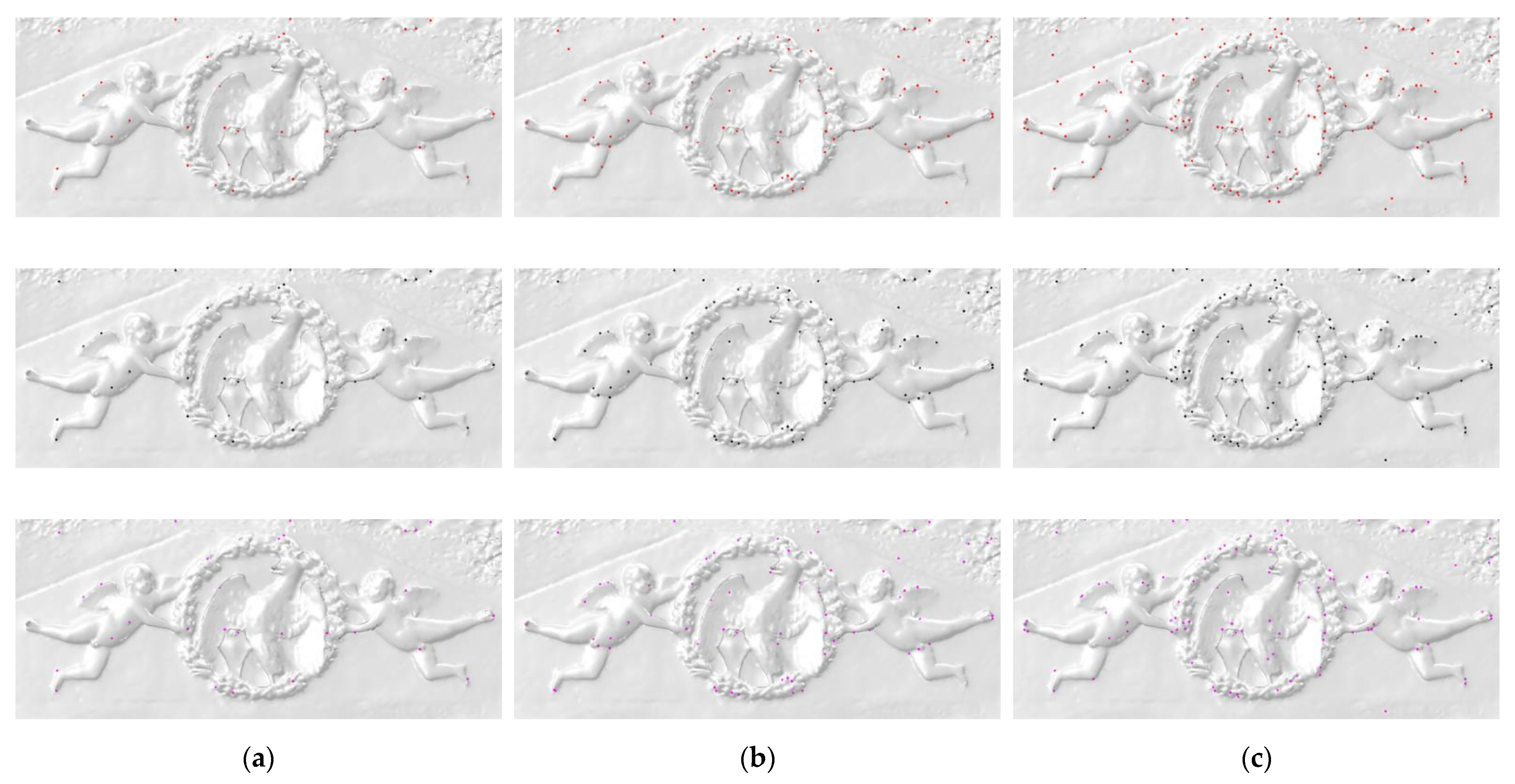
3.4. Ordered Statistics Vertex Extraction
4. Our Algorithm
4.1. Mesh Processing
4.2. Ordered Statistics Algorithm
4.3. Adaptive Mesh Quantization
4.4. Similarity Matching Procedure
4.5. Neural Networks for 3D Feature Ranking
5. Numerical Results
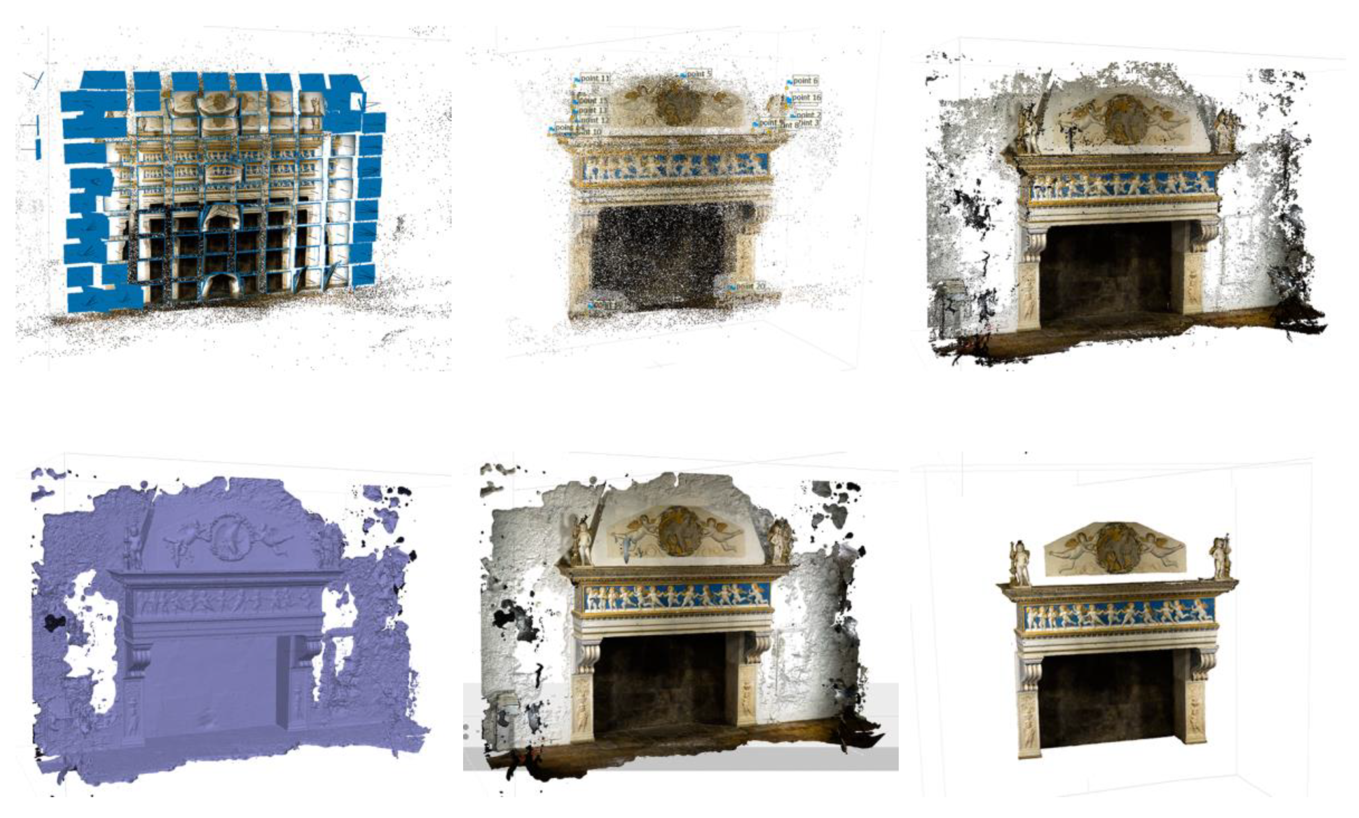
5.1. Mesh Processing Performance
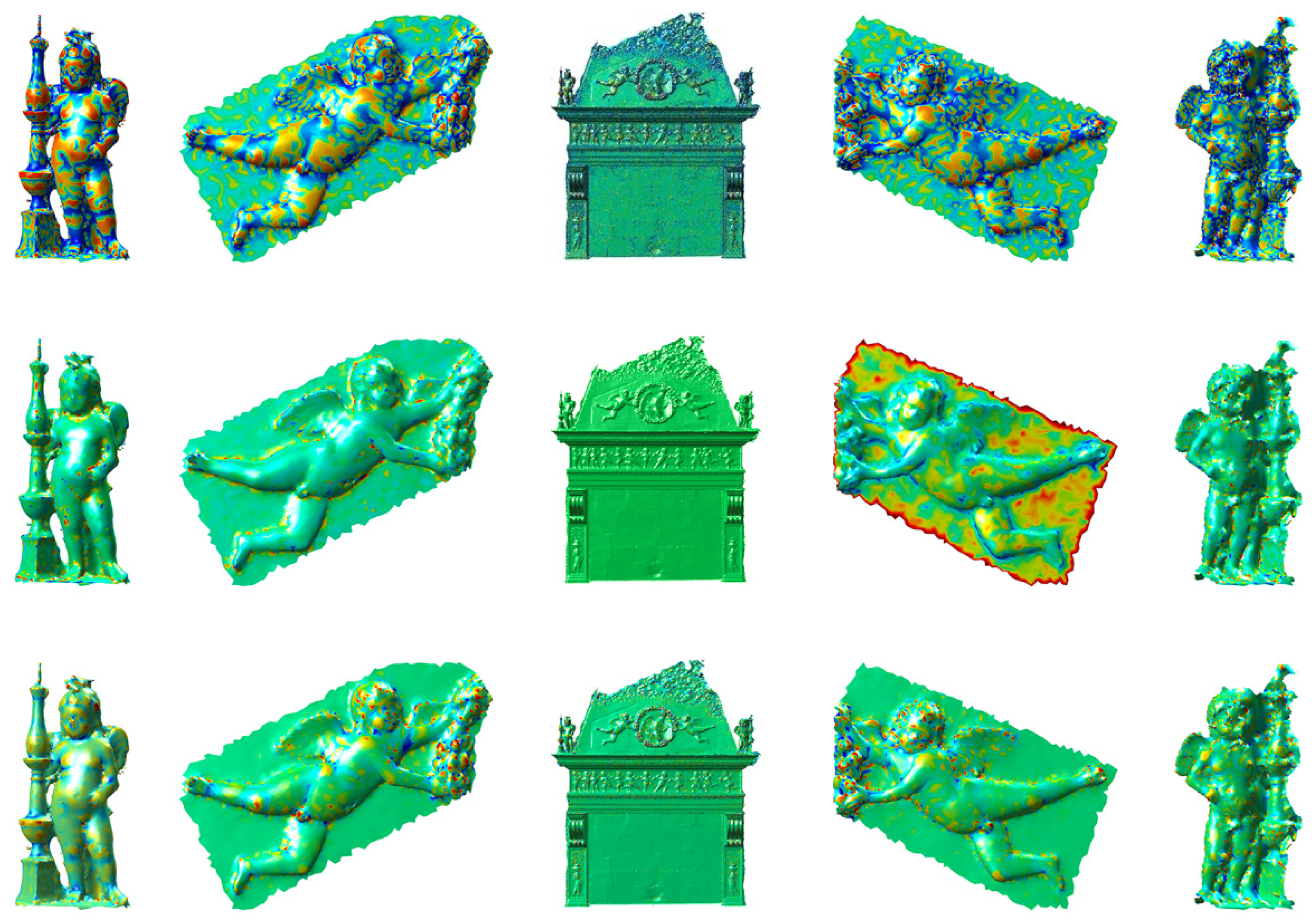
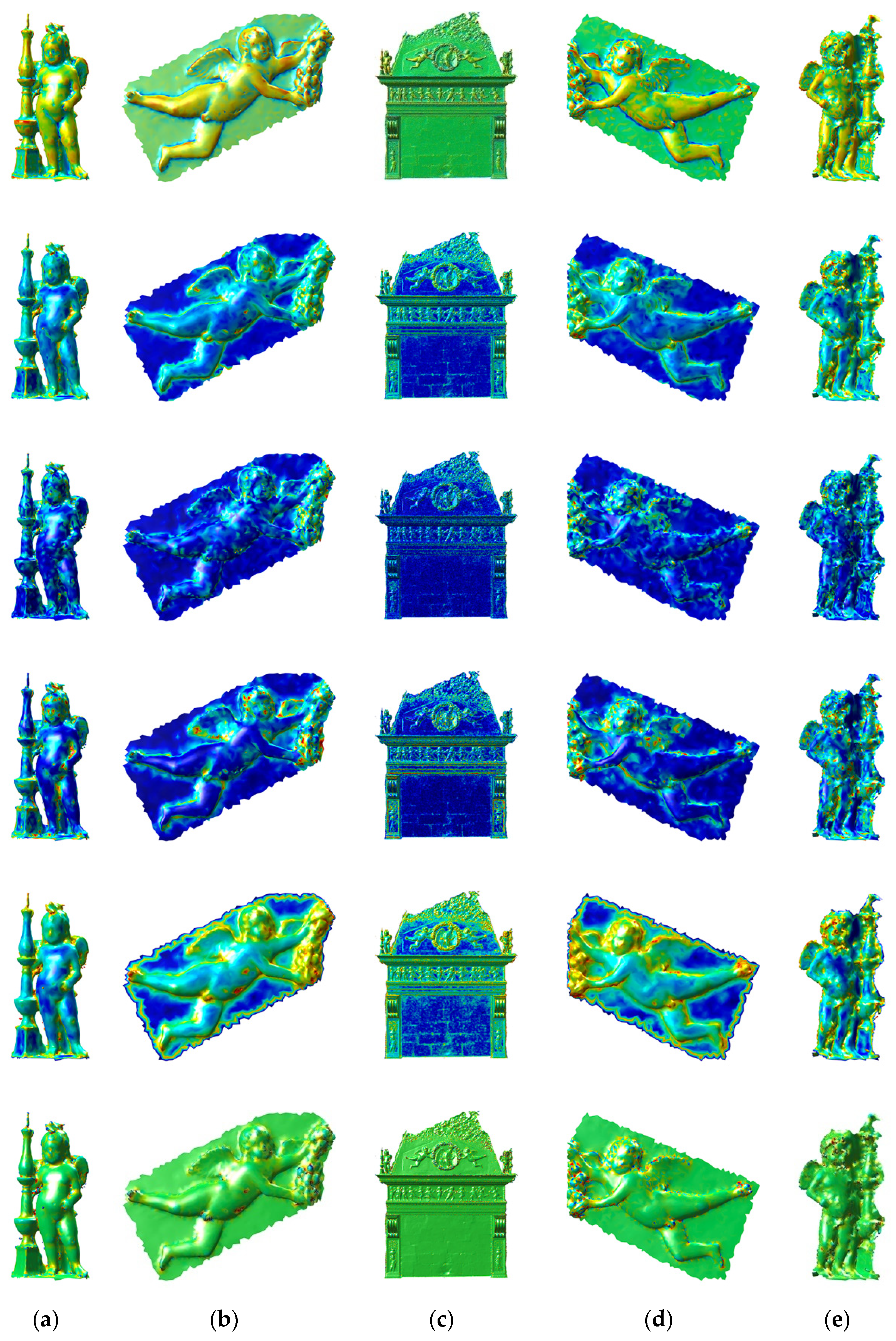
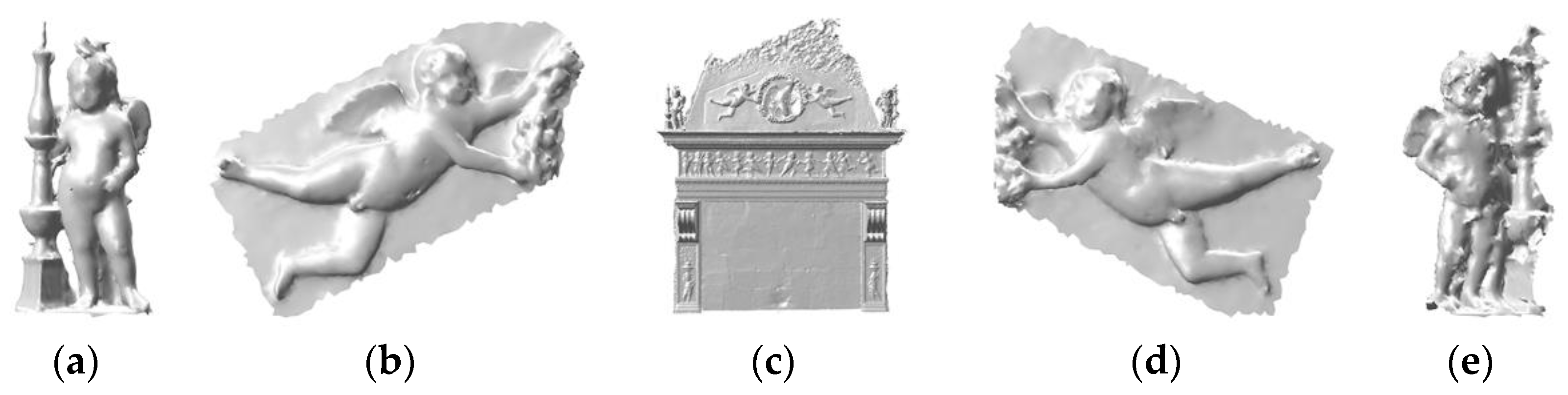
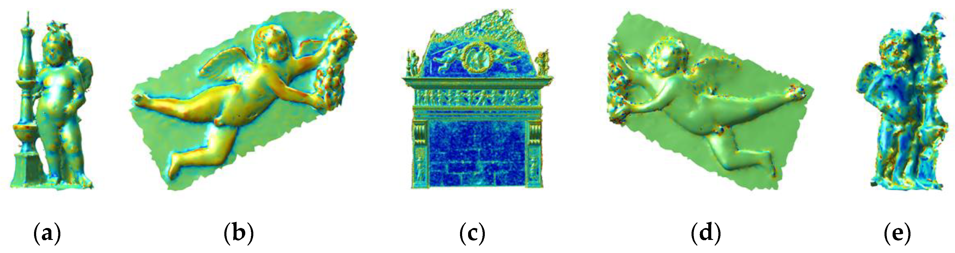
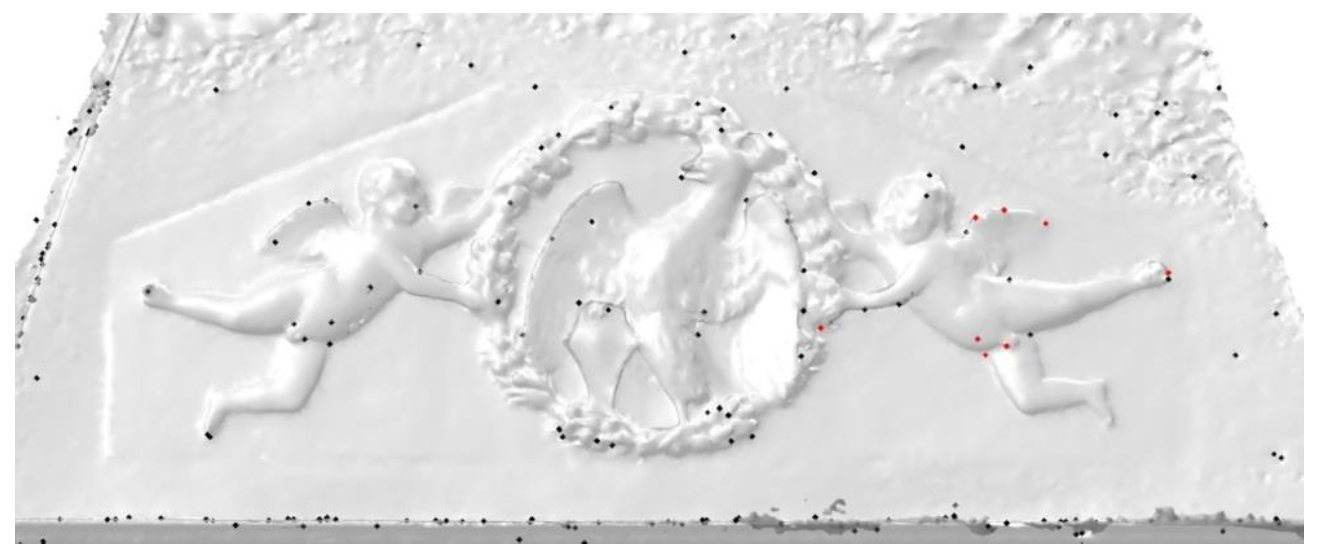
- angelo-1L.obj—the sculpture of an angel on the top-left,
- angelo-1R.obj—the symmetrical pair at the right,
- angelo-2L.obj—the left angel ornament,
- angelo-2R.obj—the symmetrical pair at the right, and
- camino degli angeli.obj—the whole fireplace 3D model.
5.2. Ordered Statistics Vertex Extraction Performance
5.3. Results of the Quantization
5.4. Matching Shapes Performance
6. Discussion, Conclusions and Future Work
Supplementary Materials
Author Contributions
Funding
Data Availability Statement
Acknowledgments
Conflicts of Interest
Appendix A. The Case Study: Description and Data Survey

| Feature | Sensor Dimension | Value | Unit | Bounding Box | Value | Unit |
|---|---|---|---|---|---|---|
| w | Length | 35.6 | mm | Length | 423 | mm |
| h | Height | 23.8 | mm | Height | 420 | mm |
| D | Target distance | 1000 | mm | Sidelap | 60 | % |
| f | Focal length | 24 | mm | Overlap | 60 | % |
| w | Horizontal image size | 6000 | pix | Sidelap | 89 | cm |
| h | Vertical image size | 3376 | pix | Overlap | 60 | cm |
| Camera resolution | (Mpix) | Displacement x | 59 | cm | ||
| pix h | Sensor pixel size (horiz.) | 0.006 | mm | Displacement y | 40 | cm |
| pix v | Sensor pixel size (vert.) | 0.007 | mm | Shooting Stations | - | |
| s | Magnification | 41.667 | no. of stations along the x axis | 7 | - | |
| Artifact Dimension | no. of stations along the y axis | 11 | - | |||
| w | Length | 148 | cm | Total of nadiral photos | 75 | - |
| h | Height | 99.17 | cm | no. of oblique x axis stations | 4 | - |
| Pixel dimension | no. of oblique y axis stations | 5 | - | |||
| w | Length | 0.247 | mm | Total of side photos | 62 | - |
| h | Height | 0.294 | mm | Total photos | 137 | - |
Appendix B
References
- Pavlidis, G.; Koutsoudis, A.; Arnaoutoglou, F.; Tsioukas, V.; Chamzas, C. Methods for 3D digitization of Cultural Heritage. J. Cult. Herit. 2007, 8, 93–98. [Google Scholar] [CrossRef] [Green Version]
- Vasic, I.; Pierdicca, R.; Frontoni, E.; Vasic, B. A New Technique of the Virtual Reality Visualization of Complex Volume Images from the Computer Tomography and Magnetic Resonance Imaging. In Augmented Reality, Virtual Reality, and Computer Graphics, 1st ed.; De Paolis, L.T., Arpaia, P., Bourdot, P., Eds.; Springer International Publishing: Cham, The Netherlands, 2021; pp. 376–391. [Google Scholar] [CrossRef]
- Furukawa, Y.; Hernández, C. Multi-View Stereo: A Tutorial. Found. Trends Comput. Graph. Vis. 2015, 9, 1–48. [Google Scholar] [CrossRef] [Green Version]
- Hartley, R.; Zisserman, A. Multiple View Geometry in Computer Vision, 2nd ed.; Cambridge University Press: New York, NY, USA, 2004. [Google Scholar] [CrossRef] [Green Version]
- Davison, A.J.; Reid, I.D.; Molton, N.D.; Stasse, O. MonoSLAM: Real-Time Single Camera SLAM. IEEE Trans. Pattern Anal. Mach. Intell. 2007, 29, 1052–1067. [Google Scholar] [CrossRef] [PubMed] [Green Version]
- Osada, R.; Funkhouser, T.; Chazelle, B.; Dobkin, D. Matching 3D models with shape distributions. In Proceedings of the International Conference on Shape Modeling and ApplicationsMay, Genova, Italy, 7–11 May 2001; IEEE: Manhattan, NY, USA, 2001; pp. 154–166. [Google Scholar] [CrossRef] [Green Version]
- Besl, P.J.; McKay, N.D. A Method for Registration of 3-D Shapes. IEEE Trans. Pattern Anal. Mach. Intell. 1992, 14, 239–256. [Google Scholar] [CrossRef]
- Itskovich, A.; Tal, A. Surface Partial Matching & Application to Archaeology. Comput. Graph. 2011, 35, 334–341. [Google Scholar] [CrossRef]
- Harary, G.; Tal, A.; Grinspun, E. Context-based Coherent Surface Completion. ACM Trans. Graph. (TOG) 2014, 33, 1–12. [Google Scholar] [CrossRef]
- McKinney, K.; Fischer, M. Generating, evaluating and visualizing construction schedules with CAD tools. Autom. Constr. 1998, 7, 433–447. [Google Scholar] [CrossRef]
- Kersting, O.; Döllner, J. Interactive 3D visualization of vector data in GIS. In Proceedings of the 10th ACM International Symposium on Advances in Geographic Information, McLean, VA, USA, 8–9 November 2002; Association for Computing Machinery: New York, NY, USA, 2002; pp. 107–112. [Google Scholar] [CrossRef] [Green Version]
- Deleart, F.; Seitz, S.M.; Thrope, C.E.; Thrun, S. Structure from motion without correspondence. In Proceedings of the IEEE Conference on Computer Vision and Pattern Recognition, CVPR 2000 (Cat. No.PR00662), Hilton Head, SC, USA, 13–15 June 2000; IEEE: Manhattan, NY, USA, 2000; Volume 2, pp. 557–564. [Google Scholar] [CrossRef]
- Van den Hengel, A.; Dick, A.R.; Thormählen, T.; Ward, B.; Torr, P.H.S. Videotrace: Rapid Interactive Scene Modelling from Video. In ACM SIGGRAPH 2007 Papers; Association for Computing Machinery: New York, NY, USA, 2007; p. 86-es. [Google Scholar] [CrossRef]
- Funkhouser, T.; Min, P.; Kazhdan, M.; Chen, J.; Halderman, A.; Dobkin, D.; Jacobs, D. A search engine for 3D models. ACM Trans. Graph. 2003, 22, 83–105. [Google Scholar] [CrossRef]
- Qin, S.; Li, Z.; Chen, Z. Similarity Analysis of 3D Models Based on Convolutional Neural Networks with Threshold. In Proceedings of the 2018 the 2nd International Conference on Video and Image Processing, Tokyo, Japan, 29–31 December 2018; Association for Computing Machinery: New York, NY, USA, 2018; pp. 95–102. [Google Scholar] [CrossRef]
- Rossignac, J. Corner-operated Tran-similar (COTS) Maps, Patterns, and Lattices. ACM Trans. Graph. 2020, 39, 1–14. [Google Scholar] [CrossRef]
- Ju, T.; Schaefer, S.; Warren, J. Mean value coordinates for closed triangular meshes. ACM Trans. Graph. 2005, 24, 561–566. [Google Scholar] [CrossRef]
- Mitra, N.J.; Pauly, M.; Wand, M.; Ceylan, D. Symmetry in 3D geometry: Extraction and applications. Comput. Graph. Forum 2013, 32, 1–23. [Google Scholar] [CrossRef]
- Chang, M.C.; Kimia, B.B. Measuring 3D Shape Similarity by Matching the Medial Scaffolds. In Proceedings of the IEEE 12th International Conference on Computer Vision Workshops, ICCV Workshops, Kyoto, Japan, 27 September–4 October 2009; IEEE: Manhattan, NY, USA, 2009; pp. 1473–1480. [Google Scholar] [CrossRef]
- Bustos, B.; Keim, D.A.; Saupe, D.; Schreck, T.; Vranic, D.V. Feature-based similarity search in 3D object databases. ACM Comput. Surv. 2005, 37, 345–387. [Google Scholar] [CrossRef] [Green Version]
- Tabia, H.; Laga, H. Covariance-Based Descriptors for Efficient 3D Shape Matching, Retrieval, and Classification. IEEE Trans. Multimed. 2015, 17, 1591–1603. [Google Scholar] [CrossRef]
- Tangelder, J.W.H.; Veltkamp, R.C. A survey of content based 3D shape retrieval methods. Multimed. Tools Appl. 2007, 39, 441–471. [Google Scholar] [CrossRef]
- Sharf, A.; Alexa, M.; Cohen-Or, D. Context-Based Surface Completion. ACM Trans. Graph. 2004, 23, 878–887. [Google Scholar] [CrossRef] [Green Version]
- Nooruddin, F.S.; Turk, G. Simplification and Repair of Polygonal Models Using Volumetric Techniques. IEEE Educ. Act. Dep. 2003, 9, 191–205. [Google Scholar] [CrossRef] [Green Version]
- Khorramabadi, D. A Walk through the Planned CS Building, 1st ed.; University of California at Berkeley: Berkeley, CA, USA, 1991. [Google Scholar]
- Chen, D.Y.; Tian, X.P.; Shen, Y.T.; Ouhyoung, M. On Visual Similarity Based 3D Model Retrieval. Comput. Graph. Forum 2003, 22, 223–232. [Google Scholar] [CrossRef]
- Vasic, B. Ordered Statistics Vertex Extraction and Tracing Algorithm (OSVETA). Adv. Electr. Comput. Eng. 2012, 12, 25–32. [Google Scholar] [CrossRef]
- Spivak, M. A Comprehensive Introduction to Differential Geometry, 3rd ed.; Publish or Perish: Los Angeles, WA, USA, 1999. [Google Scholar]
- Meyer, M.; Desbrun, M.; Schröder, P.; Barr, A.H. Discrete Differential-Geometry Operators for Triangulated 2-Manifolds. In Visualization and Mathematics III; Hege, H.C., Ed.; Springer Berlin/Heidelberg: Berlin/Heidelberg, Germany, 2003; pp. 35–57. [Google Scholar] [CrossRef] [Green Version]
- McIvor, A.M.; Valkenburg, R.J. A comparison of local surface geometry estimation methods. Mach. Vis. Appl. 1997, 10, 17–26. [Google Scholar] [CrossRef]
- Gray, R.M.; Neuhoff, D.L. Quantization. IEEE Trans. Inf. Theory 1998, 44, 2325–2383. [Google Scholar] [CrossRef]
- Vasic, B.; Vasic, B. Simplification Resilient LDPC-Coded Sparse-QIM Watermarking for 3D-Meshes. IEEE Trans. Multimed. 2013, 15, 1532–1542. [Google Scholar] [CrossRef]
- Vasic, B.; Raveendran, N.; Vasic, B. Neuro-OSVETA: A Robust Watermarking of 3D Meshes. In Proceedings of the International Telemetering Conference, Las Vegas, NV, USA, 21–24 October 2019; International Foundation for Telemetering: Las Vegas, NV, USA, 2019; Volume 55, pp. 387–396. [Google Scholar]
- Vasic, B.; Vasic, I. Angeli Similarity Research. 2021. Available online: http://iva.silicon-studio.com/AngeliSImilarityResearch.zip (accessed on 8 January 2022).


| Criterion | Description | Weight | Criterion | Description | Weight |
|---|---|---|---|---|---|
| Positive | 0.4 | Negative 1 | 0.7 | ||
| Negative | 0.8 | Positive 1 | 1.0 | ||
| Positive mean curvature | 0.6 | Negative 1 | 1.0 | ||
| Negative mean curvature | 0.7 | Maximal dihedral | 0.8 | ||
| Small theta angle | 0.8 | Minimal dihedral | 0.7 | ||
| Big theta angle | 0.2 | Gradient | 0.7 | ||
| Positive 1 | 1.0 | Gradient | 0.4 |
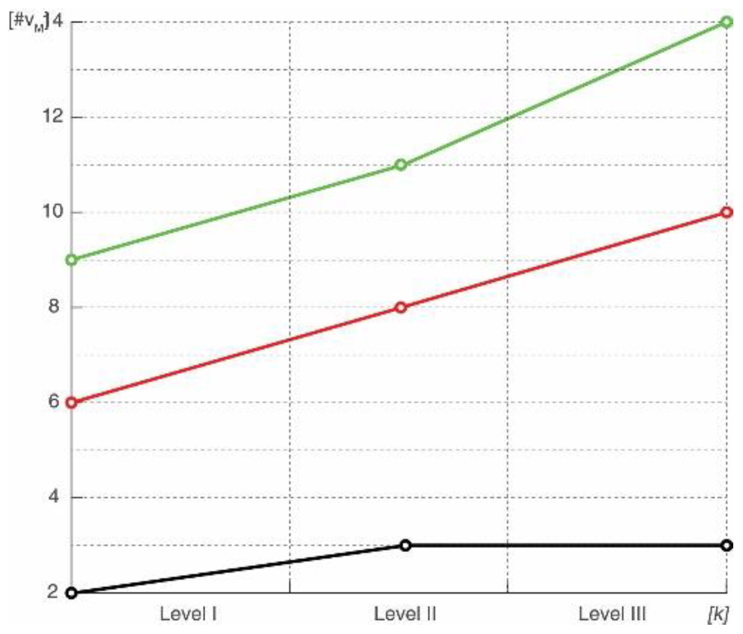
| Whole Mesh Quants 1 | Sample Quants | Tolerance Values 2 | Extracted Vertices 3 | Sample Vertices 4 | Matched Vertices |
|---|---|---|---|---|---|
| 9 × 28 × 14 | 2 × 2 × 2 | 1/2 | 737 | 6 | 3 |
| 1/6 | 653 | 3 | |||
| 1/12 | 595 | 2 | |||
| 14 × 42 × 12 | 3 × 3 × 3 | 1/2 | 1597 | 10 | 10 |
| 1/6 | 1316 | 8 | |||
| 1/12 | 1146 | 6 | |||
| 18 × 55 × 27 | 4 × 4 × 4 | 1/2 | 2687 | 15 | 14 |
| 1/6 | 2099 | 11 | |||
| 1/12 | 1777 | 9 |
Publisher’s Note: MDPI stays neutral with regard to jurisdictional claims in published maps and institutional affiliations. |
© 2022 by the authors. Licensee MDPI, Basel, Switzerland. This article is an open access article distributed under the terms and conditions of the Creative Commons Attribution (CC BY) license (https://creativecommons.org/licenses/by/4.0/).
Share and Cite
Vasic, I.; Quattrini, R.; Pierdicca, R.; Frontoni, E.; Vasic, B. A Method for Determining the Shape Similarity of Complex Three-Dimensional Structures to Aid Decay Restoration and Digitization Error Correction. Information 2022, 13, 145. https://doi.org/10.3390/info13030145
Vasic I, Quattrini R, Pierdicca R, Frontoni E, Vasic B. A Method for Determining the Shape Similarity of Complex Three-Dimensional Structures to Aid Decay Restoration and Digitization Error Correction. Information. 2022; 13(3):145. https://doi.org/10.3390/info13030145
Chicago/Turabian StyleVasic, Iva, Ramona Quattrini, Roberto Pierdicca, Emanuele Frontoni, and Bata Vasic. 2022. "A Method for Determining the Shape Similarity of Complex Three-Dimensional Structures to Aid Decay Restoration and Digitization Error Correction" Information 13, no. 3: 145. https://doi.org/10.3390/info13030145
APA StyleVasic, I., Quattrini, R., Pierdicca, R., Frontoni, E., & Vasic, B. (2022). A Method for Determining the Shape Similarity of Complex Three-Dimensional Structures to Aid Decay Restoration and Digitization Error Correction. Information, 13(3), 145. https://doi.org/10.3390/info13030145