
Multiple-Attribute Decision Making Based on Interval-Valued Intuitionistic Fuzzy Generalized Weighted Heronian Mean

Abstract
:1. Introduction
2. Preliminaries
- (1)
- (2)
- (3)
- (4)
- (1)
- Commutative law , ;
- (2)
- Distributive law , ;
- (3)
- Associative law , .
- (1)
- If , then ;
- (2)
- If , then
- (i)
- If , then ;
- (ii)
- If , then .
3. Some New Aggregation Operators for I-VIF Information
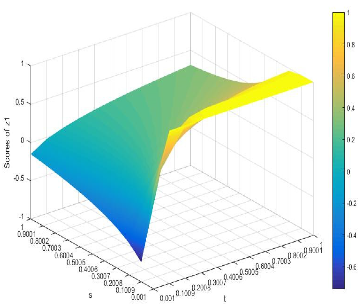
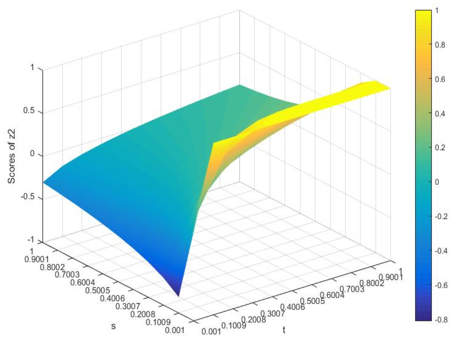
4. MADM Method Based on I-VIFGWHM Operator
4.1. MADM Method Based on I-VIFGWHM Operator
4.2. Example of MADM Based on I-VIFGWHM Operator
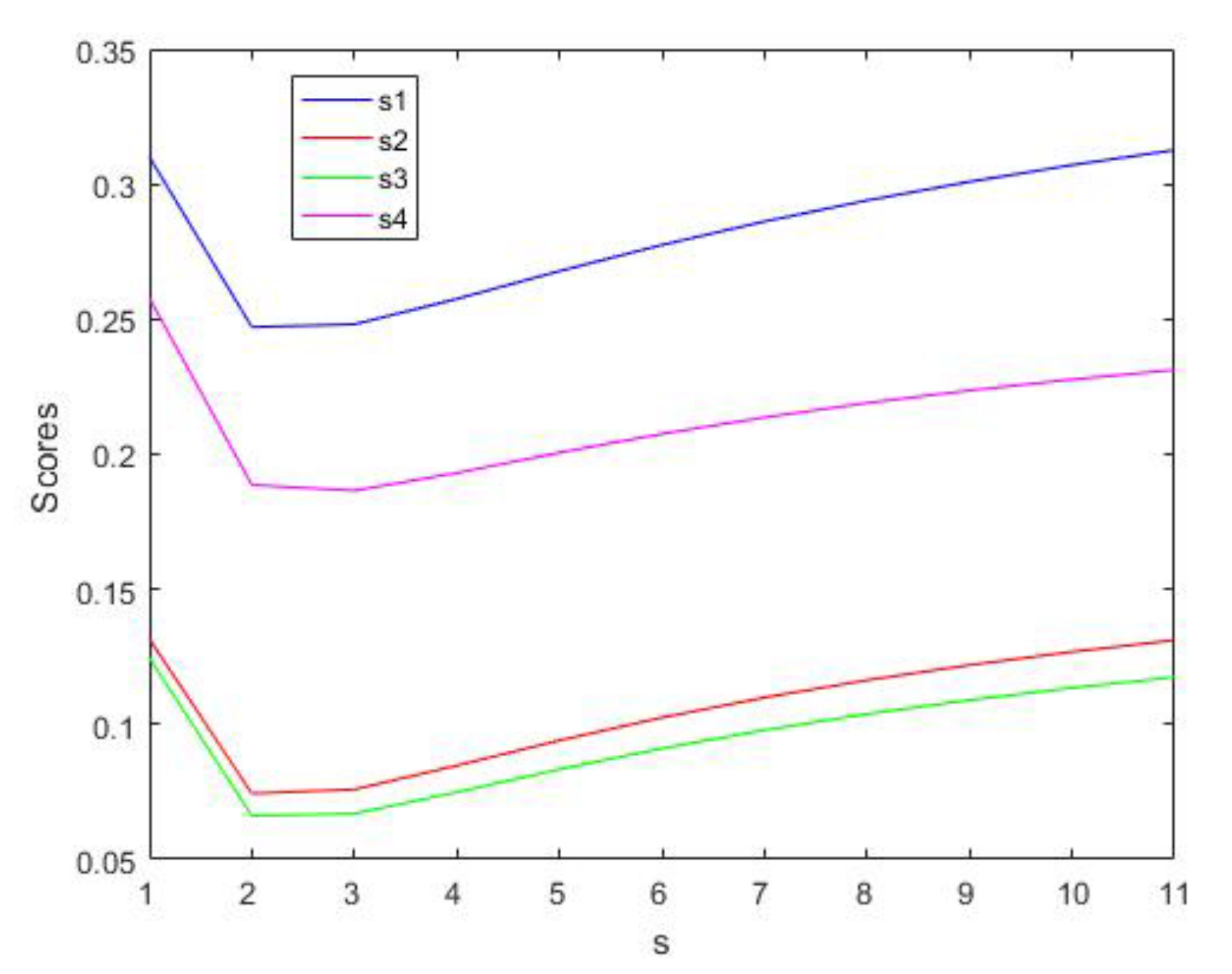
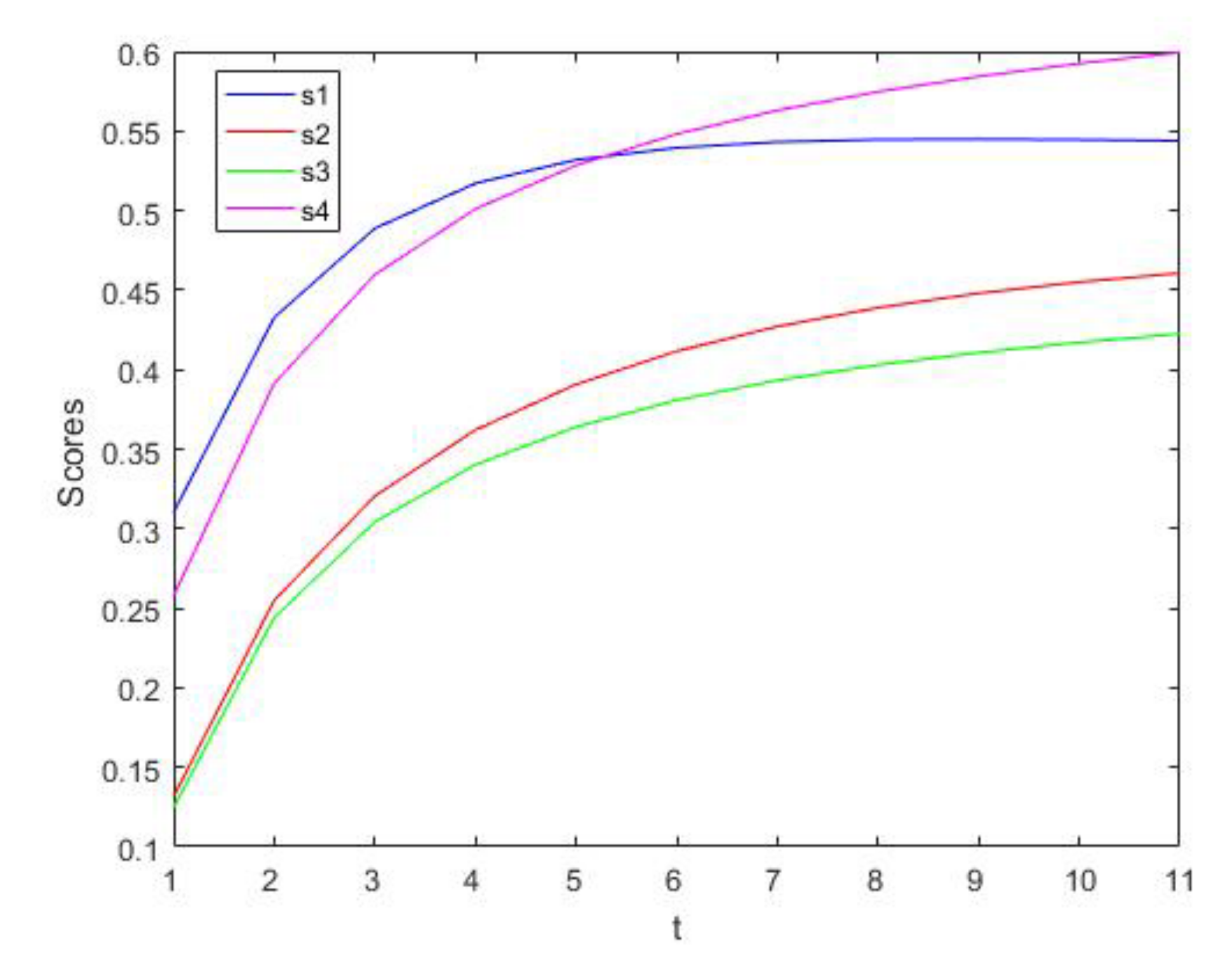
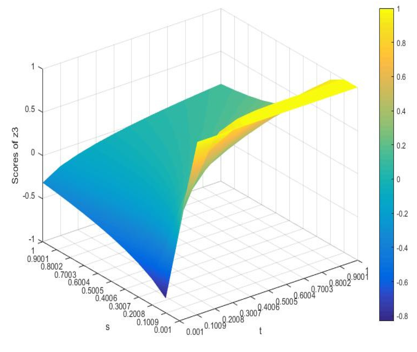
4.3. Comparison
- a
- When is fixed and , the RR is .
- b
- When is fixed and , the RR is .
- c
- When is fixed and , the RR is .
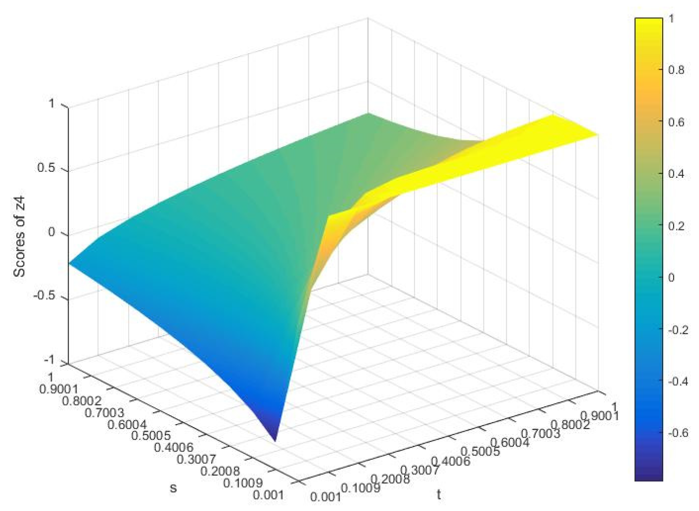
- a
- When is fixed and , the RR is .
- b
- When is fixed and , the RR is .
- c
- When is fixed and , the RR is .
- d
- When is fixed and , the RR is .
- e
- When is fixed and , the RR is .
- f
- When is fixed and , the RR is .
5. Conclusions
Author Contributions
Funding
Institutional Review Board Statement
Informed Consent Statement
Data Availability Statement
Conflicts of Interest
References
- Xu, Z. Uncertain Multiple Attribute Decision Making: Methods and Applications; Tsinghua University Press: Beijing, China, 2004. [Google Scholar]
- Liu, X.; Zhu, J.; Liu, G.; Hao, J. A multiple attribute decision making method based on uncertain linguistic Heronian mean. Math. Probl. Eng. 2013, 2013, 597671. [Google Scholar] [CrossRef]
- Ju, D.; Ju, Y.; Wang, A. Multi-attribute group decision making based on power generalized Heronian mean operator under hesitant fuzzy linguistic environment. Soft Comput. 2019, 23, 3823–3842. [Google Scholar] [CrossRef]
- Yu, D. Intuitionistic fuzzy geometric Heronian mean aggregation operators. Appl. Soft Comput. 2013, 13, 1235–1246. [Google Scholar] [CrossRef]
- Chen, Y.; Chao, R. Supplier selection using consistent fuzzy preference relations. Expert Syst. Appl. 2012, 39, 3233–3240. [Google Scholar] [CrossRef]
- Wei, G.; Zhao, X.; Lin, R.; Wang, H. Uncertain linguistic Bonferroni mean operators and their application to multiple attribute decision making. Appl. Math. Model. 2013, 37, 5277–5285. [Google Scholar] [CrossRef]
- Qin, J.; Liu, X. Approaches to uncertain linguistic multiple attribute decision making based on dual Maclaurin symmetric mean. J. Intell. Fuzzy Syst. 2015, 29, 171–186. [Google Scholar]
- Merigó, J.M. Decision-making under risk and uncertainty and its application in strategic management. J. Bus. Econ. Manag. 2015, 16, 93–116. [Google Scholar] [CrossRef] [Green Version]
- Merigó, J.M.; Casanovas, M. Induced aggregation operators in the Euclidean distance and its application in financial decision making. Expert Syst. Appl. 2011, 38, 7603–7608. [Google Scholar] [CrossRef]
- Zeng, S.; Merigó, J.M.; Palacios-Marqués, D.; Jin, H.; Gu, F. Intuitionistic fuzzy induced ordered weighted averaging distance operator and its application to decision making. J. Intell. Fuzzy Syst. 2017, 32, 11–22. [Google Scholar]
- Gong, C.; Su, Y.; Liu, W.; Hu, Y.; Zhou, Y. The distance induced OWA operator with application to multicriteria group decision making. Int. J. Intell. Syst. 2020, 22, 1624–1634. [Google Scholar]
- Zhang, Z. Geometric Bonferroni means of interval-valued intuitionistic fuzzy numbers and their application to multiple attribute group decision making. Neural Comput. Appl. 2018, 29, 1139–1154. [Google Scholar] [CrossRef]
- Wang, J.; Zhou, Y. Multi-attribute group decision-making based on interval-valued q-Rung Orthopair fuzzy power generalized Maclaurin symmetric mean operator and its application in online education platform performance evaluation. Information 2021, 12, 372. [Google Scholar] [CrossRef]
- Rong, Y.; Pei, Z.; Liu, Y. Linguistic Pythagorean Einstein operators and their application to decision making. Information 2020, 11, 46. [Google Scholar] [CrossRef] [Green Version]
- Liu, P.; Mahmood, T.; Ali, Z. Complex q-rung orthopair fuzzy aggregation operators and their applications in multi-attribute group decision making. Information 2020, 11, 5. [Google Scholar] [CrossRef] [Green Version]
- Liu, Z.; Zhao, X.; Li, L.; Wang, X.; Wang, D. A novel multi-attribute decision making method based on the double Hierarchy hesitant fuzzy linguistic generalized power aggregation operator. Information 2019, 10, 339. [Google Scholar] [CrossRef] [Green Version]
- Jin, Y.; Wu, H.; Merigó, J.M.; Peng, B. Generalized Hamacher aggregation operators for intuitionistic uncertain linguistic sets: Multiple attribute group decision making methods. Information 2019, 10, 206. [Google Scholar] [CrossRef] [Green Version]
- Mei, Y.; Peng, J.; Yang, J. Convex aggregation operators and their applications to multi-hesitant fuzzy multi-criteria decision-making. Information 2018, 9, 207. [Google Scholar] [CrossRef] [Green Version]
- Lu, X.; Ye, J. Dombi aggregation operators of linguistic cubic variables for multiple attribute decision making. Information 2018, 9, 188. [Google Scholar] [CrossRef] [Green Version]
- Xu, Y.; Shang, X.; Wang, J. Pythagorean fuzzy interaction Muirhead means with their application to multi-attribute group decision-making. Information 2018, 9, 157. [Google Scholar] [CrossRef] [Green Version]
- Tian, J.-F.; Zhang, Z.; Ha, M.-H. An additive-consistency- and consensus-based approach for uncertain group decision making with linguistic preference relations. IEEE Trans. Fuzzy Syst. 2019, 27, 873–887. [Google Scholar] [CrossRef]
- Tian, J.-F.; Ha, M.-H.; Xing, H.-J. Properties of the power-mean and their applications. AIMS Math. 2020, 5, 7285–7300. [Google Scholar] [CrossRef]
- Xing, Y.P.; Zhang, R.T.; Wang, J.; Zhu, X.M. Some new Pythagorean fuzzy Choquet–Frank aggregation operators for multi-attribute decision making. Int. J. Fuzzy Syst. 2018, 33, 2189–2215. [Google Scholar] [CrossRef]
- Wang, J.; Zhang, R.T.; Zhu, X.M.; Xing, Y.P.; Buchmeister, B. Some hesitant fuzzy linguistic Muirhead means with their application to multiattribute group decision-making. Complexity 2018, 2018, 5087851. [Google Scholar] [CrossRef] [Green Version]
- Zhang, R.T.; Wang, J.; Zhu, X.M.; Xia, M.M.; Yu, M. Some generalized Pythagorean fuzzy Bonferroni mean aggregation operators with their application to multiattribute group decision-making. Complexity 2017, 2017, 5937376. [Google Scholar] [CrossRef] [Green Version]
- Zhang, H.R.; Zhang, R.T.; Huang, H.Q.; Wang, J. Some picture fuzzy Dombi Heronian mean operators with their application to multi-attribute decision-making. Symmetry 2018, 10, 593. [Google Scholar] [CrossRef] [Green Version]
- Xu, Z. Intuitionistic Fuzzy Information Aggregation: Theory and Applications; Science Press: Beijing, China, 2008. [Google Scholar]
- Dyckhoff, H.; Pedrycz, W. Generalized means as model of compensative connectives. Fuzzy Set. Syst. 1984, 14, 143–154. [Google Scholar] [CrossRef]
- Atanassov, K.; Gargov, G. Interval-valued intuitionistic fuzzy sets. Fuzzy Set. Syst. 1989, 31, 343–349. [Google Scholar] [CrossRef]
- Xu, Z. Methods for aggregating interval-valued intuitionistic fuzzy information and their application to decision making. Control Decis. 2007, 22, 215–219. [Google Scholar]
- Garg, H. A new generalized improved score function of interval-valued intuitionistic fuzzy sets and applications in expert systems. Appl. Soft Comput. 2016, 38, 988–999. [Google Scholar] [CrossRef]
- Wei, C. Entropy measures for interval-valued intuitionistic fuzzy sets and their application in group decision-making. Math. Probl. Eng. 2015, 2015, 563745. [Google Scholar] [CrossRef] [Green Version]
- Wu, L.; Wei, G.; Wu, J.; Wei, C. Some interval-valued intuitionistic fuzzy Dombi Heronian mean operators and their application for evaluating the ecological value of forest ecological tourism demonstration areas. Int. J. Environ. Res. Public Health 2020, 17, 829. [Google Scholar] [CrossRef] [PubMed] [Green Version]
- Yu, D.; Wu, Y. Interval-valued intuitionistic fuzzy Heronian mean operators and their application in multi-criteria decision making. Afr. J. Bus. Manag. 2012, 6, 4158–4168. [Google Scholar] [CrossRef]
- Zang, Y.; Zhao, X.; Li, S. Interval-valued dual hesitant fuzzy Heronian mean aggregation operators and their application to multi-attribute decision making. Int. J. Comput. Intell. Appl. 2018, 17, 1850005. [Google Scholar] [CrossRef]


| ([0.6,0.7], [0.1,0.2]) | ([0.5,0.6], [0.2,0.3]) | ([0.4,0.5], [0.3,0.5]) | ([0.5,0.7], [0.1,0.3]) | |
| ([0.2,0.3], [0.4,0.6]) | ([0.4,0.5], [0.1,0.2]) | ([0.4,0.5], [0.3,0.5]) | ([0.4,0.5], [0.2,0.3]) | |
| ([0.3,0.4], [0.5,0.6]) | ([0.4,0.5], [0.2,0.3]) | ([0.4,0.6], [0.3,0.4]) | ([0.4,0.5], [0.2,0.3]) | |
| ([0.5,0.6], [0.3,0.4]) | ([0.6,0.7], [0.2,0.3]) | ([0.5,0.6], [0.3,0.4]) | ([0.4,0.6], [0.3,0.4]) |
| ([0.4924,0.6161],[0.1730,0.3268]) | ([0.3591,0.4615],[0.2145,0.3656]) | ([0.3801,0.5126],[0.2750,0.3805]) | ([0.5126,0.6322],[0.2664,0.3678]) | |
| ([0.3489,0.4486],[0.3487,0.5018]) | ([0.2474,0.3217],[0.3997,0.5405]) | ([0.2625,0.3601],[0.4589,0.5529]) | ([0.3601,0.4578],[0.4505,0.5422]) | |
| ([0.4949,0.6188],[0.1712,0.3224]) | ([0.3645,0.4652],[0.2107,0.3557]) | ([0.3812,0.5150],[0.2713,0.3757]) | ([0.5150,0.6331],[0.2656,0.3669]) | |
| ([0.5546,0.7131],[0.0099,0.1686]) | ([0.4373,0.5647],[0.0019,0.0901]) | ([0.4385,0.6511],[0.0576,0.1978]) | ([0.6511,0.7978],[0.0618,0.2022]) | |
| ([0.4836,0.6013],[0.2076,0.3414]) | ([0.3540,0.4474],[0.2529,0.3773]) | ([0.3643,0.4903],[0.3053,0.4000]) | ([0.4903,0.5972],[0.3088,0.4028]) | |
| ([0.5022,0.6215],[0.1893,0.3203]) | ([0.3707,0.4660],[0.2315,0.3515]) | ([0.3791,0.5097],[0.2838,0.3780]) | ([0.5097,0.6172],[0.2887,0.3828]) |
| Scheme Sorting Results | |||||
|---|---|---|---|---|---|
| 0.3043 | 0.1202 | 0.1185 | 0.2553 | ||
| −0.0265 | −0.1855 | −0.1946 | −0.0874 | ||
| 0.3101 | 0.1316 | 0.1246 | 0.2578 | ||
| 0.5445 | 0.4551 | 0.4171 | 0.5924 | ||
| 0.2679 | 0.0856 | 0.0747 | 0.188 | ||
| 0.3071 | 0.1269 | 0.1135 | 0.2277 |
| Methods | Score Value | Ranking Result |
|---|---|---|
| The method based on IIFWA | , , , | |
| The method based on IIFWG | , , , | |
| Yu’s [34] method ) | , , , | |
| The proposed method ) | , , , |
Publisher’s Note: MDPI stays neutral with regard to jurisdictional claims in published maps and institutional affiliations. |
© 2022 by the authors. Licensee MDPI, Basel, Switzerland. This article is an open access article distributed under the terms and conditions of the Creative Commons Attribution (CC BY) license (https://creativecommons.org/licenses/by/4.0/).
Share and Cite
Hu, X.; Yang, S.; Zhu, Y.-R. Multiple-Attribute Decision Making Based on Interval-Valued Intuitionistic Fuzzy Generalized Weighted Heronian Mean. Information 2022, 13, 138. https://doi.org/10.3390/info13030138
Hu X, Yang S, Zhu Y-R. Multiple-Attribute Decision Making Based on Interval-Valued Intuitionistic Fuzzy Generalized Weighted Heronian Mean. Information. 2022; 13(3):138. https://doi.org/10.3390/info13030138
Chicago/Turabian StyleHu, Ximei, Shuxia Yang, and Ya-Ru Zhu. 2022. "Multiple-Attribute Decision Making Based on Interval-Valued Intuitionistic Fuzzy Generalized Weighted Heronian Mean" Information 13, no. 3: 138. https://doi.org/10.3390/info13030138
APA StyleHu, X., Yang, S., & Zhu, Y.-R. (2022). Multiple-Attribute Decision Making Based on Interval-Valued Intuitionistic Fuzzy Generalized Weighted Heronian Mean. Information, 13(3), 138. https://doi.org/10.3390/info13030138