Abstract
Due to the complexity and uncertainty of objective things, interval-valued intuitionistic fuzzy (I-VIF) numbers are often used to describe the attribute values in multiple-attribute decision making (MADM). Sometimes, there are correlations between the attributes. In order to make the decision-making result more objective and reasonable, it is often necessary to take the correlation factors into account. Therefore, the study of MADM based on the correlations between attributes in the I-VIF environment has important theoretical and practical significance. Thus, in this paper, we propose new operators (AOs) for I-VIF information that are able to reflect the completeness of the information, attribute relevance, and the risk preference of decision makers (DMs). Firstly, we propose some new AOs for I-VIF information, including I-VIF generalized Heronian mean (I-VIFGHM), I-VIF generalized weighted Heronian mean (I-VIFGWHM), and I-VIF three-parameter generalized weighted Heronian mean (I-VIFTPGWHM). The properties of the obtained operators, including their idempotency, monotonicity, and boundedness are studied. Furthermore, an MADM method based on the I-VIFGWHM operator is provided. Finally, an example is provided to explain the rationality and feasibility of the proposed method.
1. Introduction
MADM is an important branch of modern decision-making theory [1]. Its theory and method are widely used in many fields, such as those related to the economy, management, engineering, and the military [1,2,3,4,5,6,7,8,9,10,11,12,13,14,15,16,17,18,19,20,21]. Effective attribute value integration is a core problem of MADM. Scholars have developed many AOs [22,23,24,25,26,27,28]. The generalized mean (GM) was proposed as a connective operator by Dyckhoff and Pedrycz [28]. This operator makes it easy to model the compensation degree, naturally including the minimum and maximum operators along with the arithmetic and geometric means as special examples. The GM can not only express the preferences of the DMs, but it can also take the decision information from the perspective of the whole into account. Therefore, scholars have paid attention to GM research.
With the increasing complexity of the social and economic environment, the decision-making problems that are experienced in various fields of people’s lives and during production are becoming more and more complex. It is often difficult for DMs to provide evaluation information in the form of an accurate value. Zadel put forward the fuzzy set concept, which states the uncertainty and fuzziness of things through membership. Subsequently, Atanassov developed the fuzzy set and put forward the concept of the intuitionistic fuzzy set, which describes the uncertainty and fuzziness of things through the non-membership degree and membership degree. Because of the complicacy and nondeterminacy of things, it is sometimes difficult to express the non-membership degree and membership degree of intuitionistic fuzzy sets using real values, and it is more suitable to express them in the form of interval-valued numbers [27]. Therefore, Atanassov and Gargov [29] extended the intuitionistic fuzzy set to the I-VIF set, and then the concepts of the I-VIF number, score function of the I-VIF number, and exact function of the I-VIF number were put forward [30]. With the introduction of I-VIF number ranking method [30], the I-VIF information MADM method has become more and more important. Garg [31] presented a new generalized improved score function and an I-VIF set-based method to solve the MCDM problem. Wei [32] proposed two new entropy measures based on the cosine function for intuitionistic fuzzy sets and I-VIF sets, which were applied to solve multi-criteria fuzzy group decision-making problems.
At present, many AOs assume that attributes are mutually independent. In real decisions, however, attributes are often interrelated. Therefore, more and more experts and scholars study the MADM with interrelated attributes. The Heronian mean AO is an important AO that considers the correlations between attributes. Wu [33] produced some Dombi Heronian mean AOs with I-VIF numbers and two MADM methods based on the I-VIF-weighted Dombi Heronian mean AO and interval-valued intuitionistic-weighted Dombi geometric Heronian mean AO. Yu [34] proposed a generalized I-VIF Heronian mean and a MCDM method based on this operator. Zang [35] proposed the interval-valued dual hesitant fuzzy Heronian mean AO and the interval-valued dual hesitant fuzzy geometric Heronian mean AO.
Therefore, the study of MADM based on the correlations between attributes in the I-VIF environment has important theoretical and practical significance. Thus, in this paper, we propose some new AOs for I-VIF information, including the I-VIFGHM, I-VIFGWHM, and I-VIFTPGWHM. They have the virtues of both the Heronian mean and the GM and can reflect the completeness of information, attribute relevance, and the risk preference of DMs.
The rest of the article is described below. In Section 2, some basic notions are introduced. In Section 3, some new AOs for I-VIF information are proposed, including the I-VIFGHM, I-VIFGWHM, and I-VIFTPGWHM. The properties of the obtained operators are studied, including their idempotency, monotonicity and boundedness. In Section 4, the MADM method based on the I-VIFGWHM operator is provided, and using an example, the proposed method is compared with the existing MADM methods. In Section 5, we provide a summary and prospects for future work.
2. Preliminaries
Definition 1.
[29] Let be a nonempty set, and be the I-VIF set, where , and , .
If and , then the I-VIF sets degenerate into intuitionistic fuzzy sets.
Definition 2.
[30] Let be a nonempty set, be a I-VIF set, and be the I-VIF number and be abbreviated as , where and .
Definition 3.
[30] Let , , and be three I-VIF numbers, , creating the following algorithms:
- (1)
- (2)
- (3)
- (4)
Theorem 1.
[30] Let , , and be three I-VIF numbers, and let all of the operation results in Definition 3 continue to be I-VIF numbers.
Theorem 2.
[30] Let , , and be three I-VIF numbers, , meaning that the following algorithms hold:
- (1)
- Commutative law , ;
- (2)
- Distributive law , ;
- (3)
- Associative law , .
To rank the I-VIF numbers, Xu [30] introduced the score function and exact function to calculate the score and accuracy of the I-VIF number , resulting in the order relationship between two I-VIF numbers, and :
Definition 4.
[30] Let any two I-VIF numbers be and , and then
- (1)
- If , then ;
- (2)
- If , then
- (i)
- If , then ;
- (ii)
- If , then .
3. Some New Aggregation Operators for I-VIF Information
In this section, we propose some new AOs for I-VIF information, including the I-VIFGHM, I-VIFGWHM, and I-VIFTPGWHM.
Definition 5.
Letbe a set of nonnegative real numbers, whereand,is the weight of, and,. Then
is the generalized weighted Heronian mean, where.
Definition 6.
Let, be a set of I-VIF numbers, and. Then,
is the I-VIFGHM.
Theorem 3.
Let, be a set of I-VIF numbers. If and then the result aggregated by the operator is still an I-VIF number, and
Proof.
Using the operation laws of the I-VIF number, we obtain
then
and
that is,
and then,
Since
and, for all , we obtain
The proof is complete. □
Next, we will determine some properties of the operator.
Property 1.
(Idempotency) Suppose thatand,. Then,
Property 2.
(Monotonicity) Let,be two sets of I-VIFnumbers,where,andthen,
Proof.
On the one hand, if , , , then , and since we obtain
then
Therefore,
resulting in
Similarly, it can be determined that
On the other hand, for all since , then , and since , then , , ,
Similarly, it can be determined that
According to (3), (4), (5), and (6), we have
and
Let , , and use and to represent the scores of and respectively. Then,
From (7) and (8), we can determine that . Then,
That is, the monotonicity is valid.
The proof is complete. □
Property 3.
(Boundedness) Let() be a set of I-VIF numbers, let
and let
then
Proof.
Using Property 1, we obtain
and , Then, using Property 2, we have
Therefore, Property 3 can be proven. □
Next, the operator is presented.
Definition 7.
Let, be a set of I-VIF numbers.The weightshould satisfy,and let. If, then
is the.
Theorem 4.
Let()be a set of I-VIF numbers andthe weight satisfy . If , then the result aggregated by the operator is still an I-VIF number, and
Proof.
By the operation laws of I-VIF number, we achieve
then
and
that is,
and
Since
and for all , , we obtain
The proof is complete. □
Next, we will present some of the properties of the operator.
Property 4.
(Idempotency) For, if, then
Property 5.
(Monotonicity) Suppose thatand() are two sets of I-VIF numbers, where,, and,. Then
Proof.
On the one hand, since , ,, then , and since , we achieve
Then,
Therefore,
As such, we have
Similarly, we can obtain
On the other hand, for , since , then , and since , then , ,
Similarly, we can obtain
According to (9), (10), (11), and (12), we have
and
Let , , and use and to represent the scores of and respectively. Then
From (13) and (14), we were able to determine that . Then
that is, the monotonicity is valid.
The proof is complete. □
Property 6.
(Boundedness) Let() be a set of I-VIF numbers, let
and let
then
Proof.
Using Property 4, we find
and . Then, from Property 5, we have
Therefore, Property 6 can be proven. □
Definition 8.
Let () be a set of I-VIF numbers, the weight satisfy , and let . If , then
is the I-VIFTPGWHM.
Theorem 5.
Let () be a set of I-VIF numbers and the weight satisfy . If , then the result aggregated by the I-VIFTPGWHM operator is still the I-VIF number, and
4. MADM Method Based on I-VIFGWHM Operator
In this section, we provide an MADM method based on the I-VIFGWHM operator. Then, using an example, we compare the proposed method with existing MADM methods. The rationality and feasibility of this method are explained, and the effect of the parameters on the decision results is discussed.
4.1. MADM Method Based on I-VIFGWHM Operator
For an MADM problem, assume that the scheme set is , the attribute set is , and the attribute weight vector is , where , and . I-VIF sets are used to represent the characteristic information of scheme ,
where , represents the degree to which does not satisfy attribute , and satisfies attribute , respectively, and , , and .
If and , then the corresponding I-VIF number is , , , and the I-VIF decision matrix is obtained.
The following list indicates the decision-making steps.
Step 1. For the data type in the scheme set, normalize the decision matrix into according to the following formula:
where is the complement of , that is, .
Step 2. I I-VIFGWHM operator is then used to integrate the characteristic information () of for all of its attributes (), to obtain the comprehensive interval-valued attribute value , of scheme .
Step 3. The score value (SV) and accuracy of the comprehensive interval-valued attribute value of each scheme are calculated from the score function and the exact function, respectively.
Step 4. Using the SV and accuracy , each scheme () is sorted, and the best scheme (BS) is obtained.
4.2. Example of MADM Based on I-VIFGWHM Operator
To explain the rationality and feasibility of the MADM method proposed in this paper, using the Example in reference [34], we compare the decision-making results with other methods.
Example. Assume that a high technology company manufacturing electronic goods has plans to evaluate and select a USB connector supplier. Four suppliers ,, and are selected as candidates. Four evaluation standards are taken into account, including finance (), performance (), technology (), and organizational culture (). The indicator weight vector is obtained by . The evaluation information on the projects under the factors are represented by the I-VIF numbers (I-VIFNs) and are listed in Table 1.

Table 1.
The I-VIF decision matrix.
Now, we will demonstrate the process for determining the best supplier in terms of the proposed method.
Step 1. All of the attribute values are of the benefit type; therefore, the decision attribute matrix does not need to be normalized.
Step 2. When the values of the parameters and , the aggregated I-VIFNs can be found using the I-VIFGWHM operator and are displayed in Table 2.

Table 2.
The aggregated IIFNs for different .
Step 3. The corresponding SVs are calculated from the score function and are listed in Table 3.

Table 3.
Scheme sorting results for different .
Step 4 Using the SVs, each scheme is sorted. Additionally, the sorted schemes are listed in Table 3.
From Table 3, it can be observed that the scheme-ranking results (RRs) are relatively stable with the changes in the values of the parameters and .
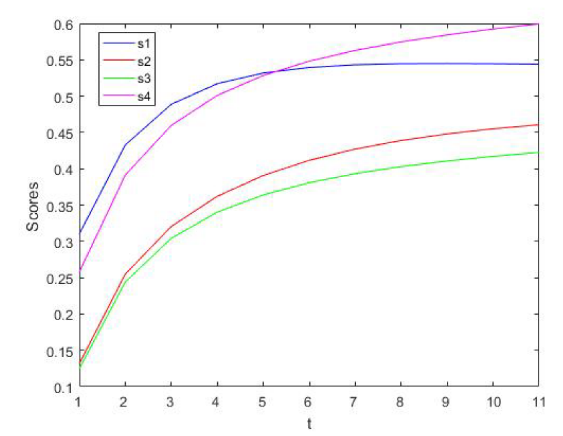
Keep the values of parameter unchanged and let take values from 1 to 11. The score change that takes place in each scheme can be obtained and are as displayed in Figure 1.

Figure 1.
, .
From Figure 1, it can be seen that when and is fixed, alternative one () is the BS. If is fixed and , then alternative four () is the BS. When the values of parameter increase, the SVs also increase.
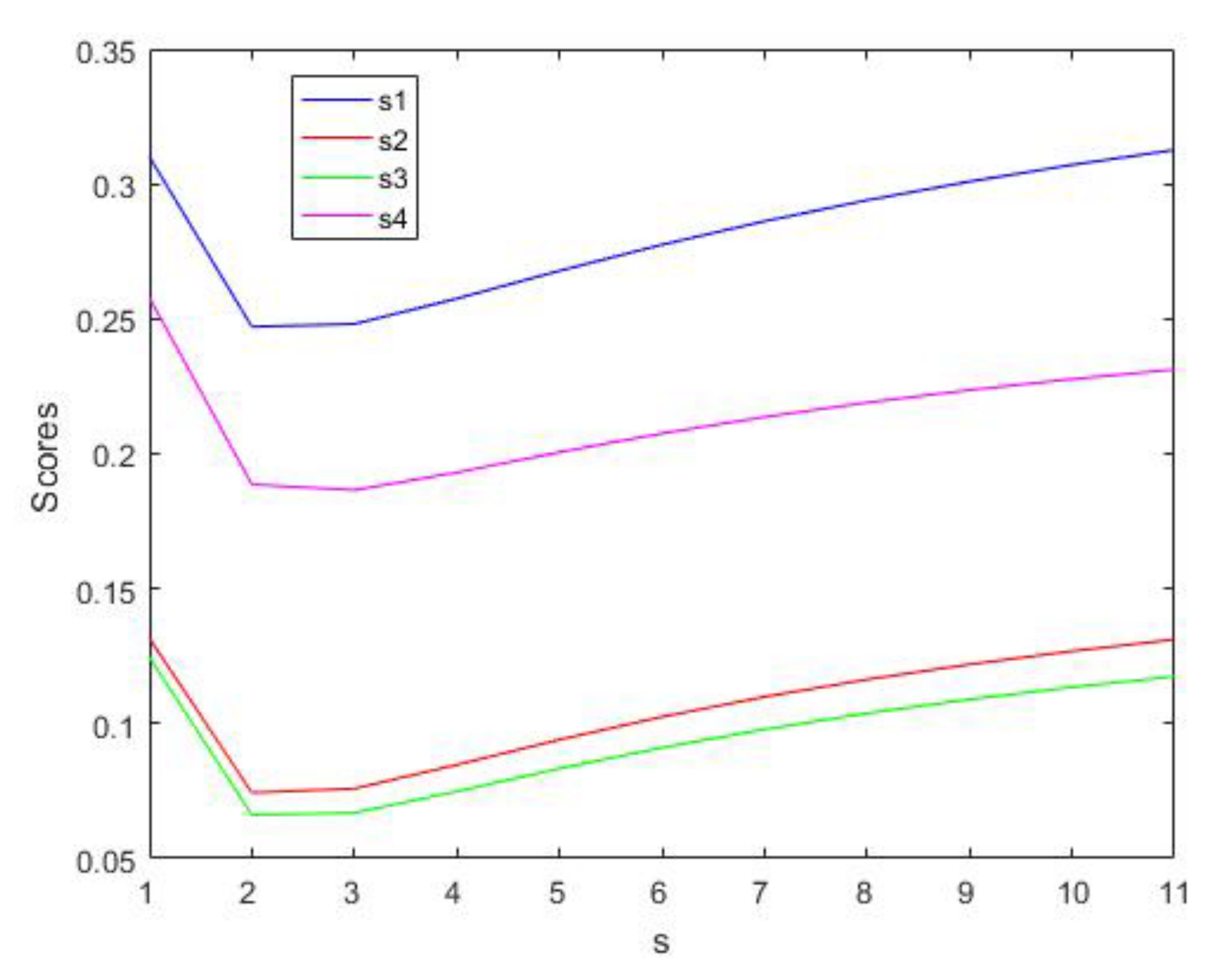
Keep the values of parameter unchanged , and let take values from 1 to 11. The score change for each scheme can be obtained and are as displayed in Figure 2.
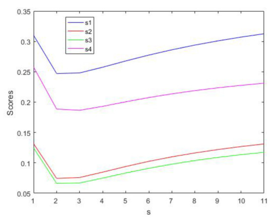
Figure 2.
, .
Figure 2 displays that when the value of remains unchanged and increases, scheme one () is always the BS.
From Figure 1 and Figure 2 we can find that the SVs of the four schemes increase when the values of parameters and increase. In practical decision-making, DMs can choose different parameter values in terms of their own risk preference. Optimistic DMs can choose larger parameters, while pessimistic DMs can choose smaller parameters.
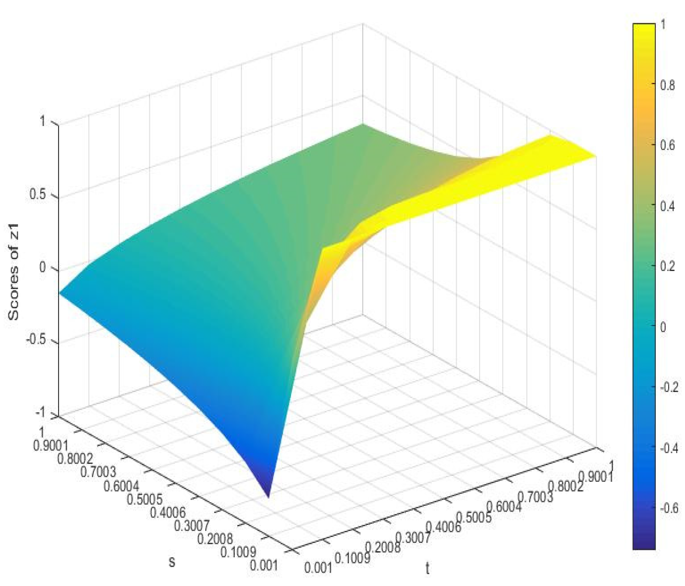
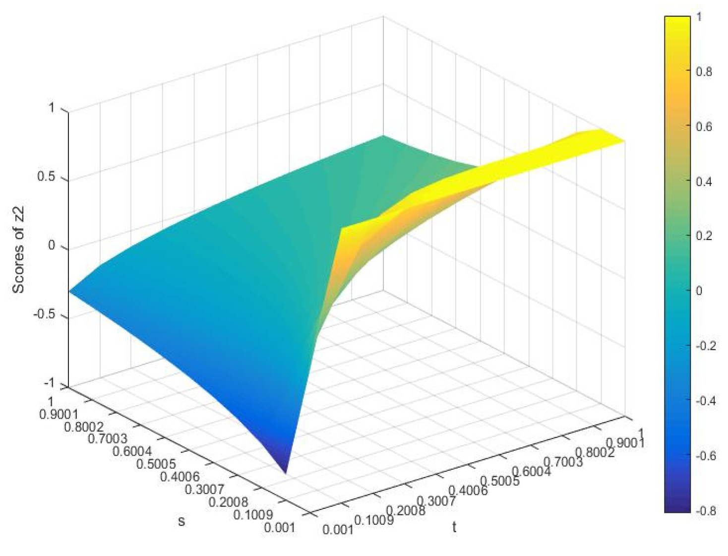
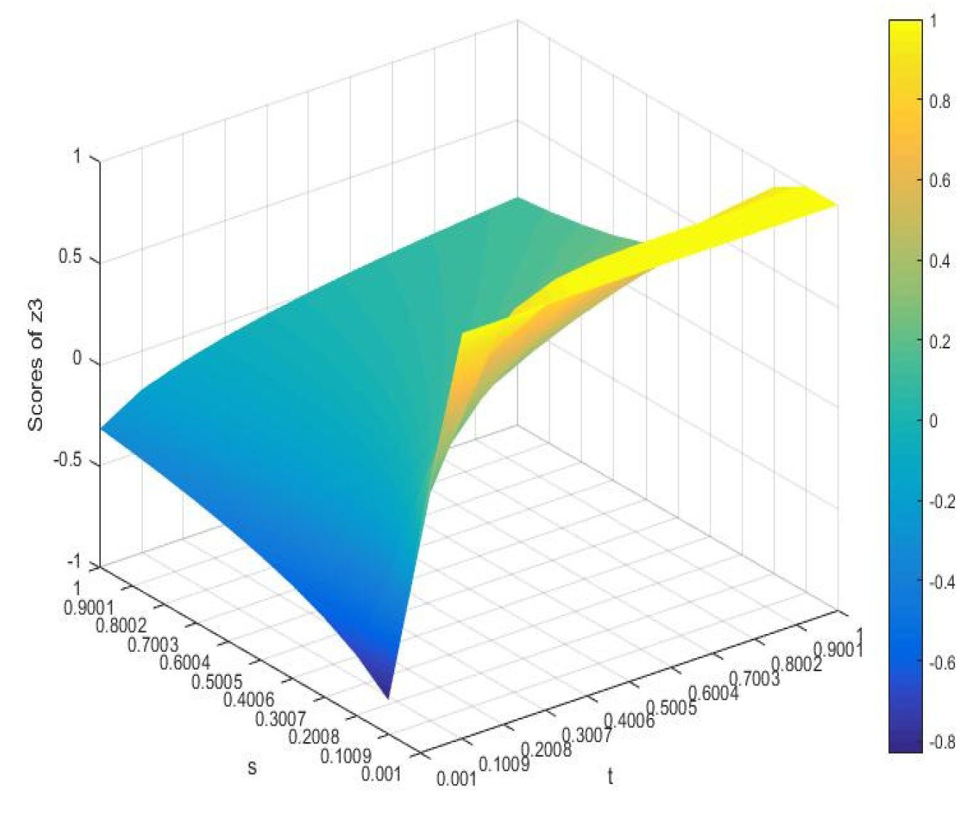
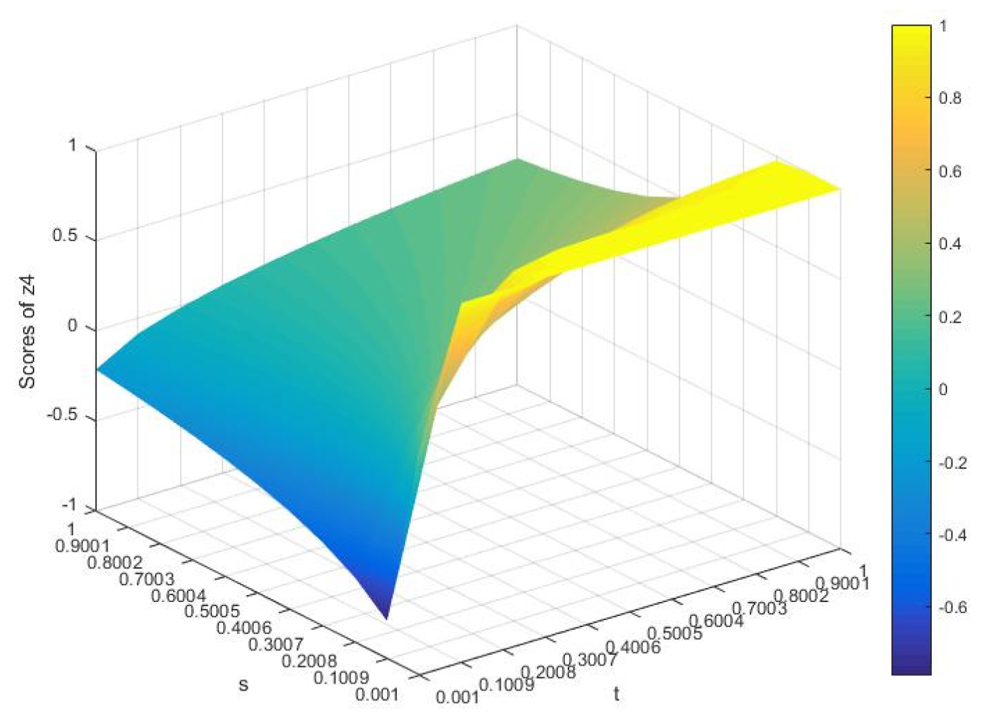
As and change, the SVs of the four schemes change are listed in Figure 3, Figure 4, Figure 5 and Figure 6.
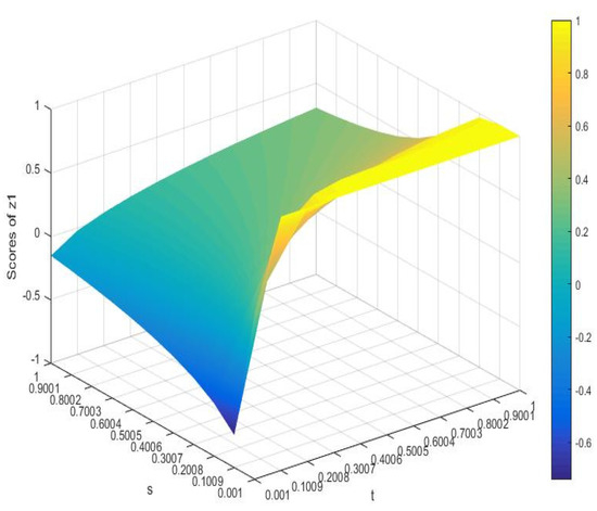
Figure 3.
Score values of scheme 1.
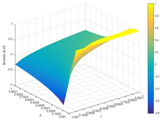
Figure 4.
Score values of scheme 2.
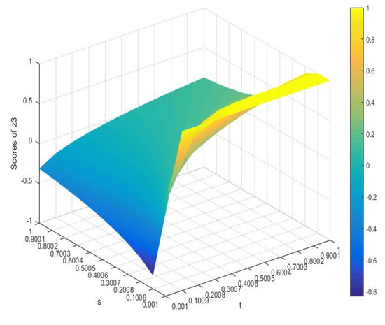
Figure 5.
Score values of scheme 3.
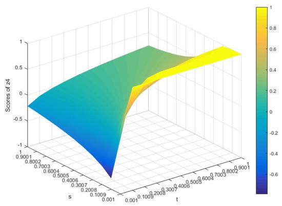
Figure 6.
Score values of scheme 4.
To sum up, we can see that the SVs will also change with the change of and , indicating that the decision-maker’s parameter choice affects the SVs. Thus, in the DM process, the appropriate parameters can be selected in terms of the risk preference of DMs. The results demonstrate the stability and flexibility of the given approach in Section 4.1.
4.3. Comparison
In this section, using the above example, we compare the obtained method with other methods, including the interval-valued intuitionistic fuzzy weighted average operator (IIFWA) [27], the interval-valued intuitionistic fuzzy weighted geometric operator (IIFWG) [27], and the method created by Yu [34] based on the generalized I-VIF weighted Heronian mean AO.
It can be seen from Table 4 that when the parameters and select a specific value, the best scheme is obtained using the method proposed in this paper, and that scheme is the same as the one obtained using the method based on the IIFWA, the method based on the IIFWG, and Yu’s [34] method (). The scheme ranking of each method is different from that of the method based on the IIFWG. In order to facilitate the list, the above table only provides the results of the comparison of the methods during parameter selection. Next, when the parameters change, the scheme RRs obtained by the proposed method and Yu’s [34] method are further compared.

Table 4.
Comparison results.
From Figure 1 and Figure 2, it can be seen that the different SVs of the alternatives can be acquired when parameters changed. The obtained RRs are as follows:
- a
- When is fixed and , the RR is .
- b
- When is fixed and , the RR is .
- c
- When is fixed and , the RR is .
From reference [34], we can see that different SVs of the alternatives can be acquired when parameters , are varied. The RRs are as follows:
- a
- When is fixed and , the RR is .
- b
- When is fixed and , the RR is .
- c
- When is fixed and , the RR is .
- d
- When is fixed and , the RR is .
- e
- When is fixed and , the RR is .
- f
- When is fixed and , the RR is .
From the above comparison, we can see that when the parameters take certain values, the scheme RRs that are obtained are different from that obtained by the method based on the IIFWA and the method based on IIFWG. The main reason for this is that the proposed method and Yu’s [34] method consider the correlations between attributes, while the method based on the IIFWA and the method based on the IIFWG assume that the attributes are independent of each other. Therefore, for the MADM problem regarding the correlations between attributes, the proposed method and Yu’s [34] method are more reasonable. Based on the results of the above comparison, it can also be observed that the scheme RRs of the proposed method and Yu’s [34] method are different as the parameters changes. The results obtained by the method provided in this paper are relatively stable. However, the BS that was obtained by the two methods belongs scheme one () or scheme four ().
To sum up, the results illustrate the flexibility and stability of the proposed methods. As such, the proposed methods are effective and feasible and are sufficient to deal with practical MADM problems. However, this is only a case study. The above conclusion can only explain that the method proposed in this paper is relatively stable in this specific case, but this does not mean that this method is better than other methods in other cases. In fact, each method has a specific application environment in which it is appropriate.
5. Conclusions
In this paper, the Heronian mean is further extended in the I-VIF environment. Some new AOs are proposed for I-VIF information. The properties of the obtained operators, including their idempotency, monotonicity, and boundedness properties, are discussed. On these bases, a MADM method that is based on the I-VIFGWHM operator was obtained, and an example was analyzed.
From the example analysis, it can be observed that the proposed method can reflect the correlations between attributes, and decision makers can choose different parameters according to their own risk preference. In actual decision-making applications, decision-makers need to evaluate decision-making objects from multiple perspectives and not only consider the interaction between attributes, but also the overall information of the decision objects as well as the risk preferences of decision makers. As such, this method can better meet the various needs of decision-makers.
The research in this paper has certain limitations. In the method propsed in this paper, only a case analysis is used to illustrate how this method is valuable in this case, but this does not mean that it is better than other methods in other cases.
We also have some suggestions for decision makers. Decision makers can choose different and parameter values based on their own risk preference. Optimistic decision makers can choose larger parameters, and pessimistic decision makers can choose smaller parameters. In future research, we will study other applications of the method proposed in this paper and will provide a more indepth generalization of the operator in other environments.
Author Contributions
Conceptualization, X.H.; methodology, X.H. and Y.-R.Z.; software, X.H.; formal analysis, X.H.; writing—original draft preparation, X.H.; writing—review and editing, X.H.; supervision, S.Y.; project administration, S.Y.; funding acquisition, Y.-R.Z. All authors have read and agreed to the published version of the manuscript.
Funding
This research was funded by the Fundamental Research Funds for the Central University, grant number MS117.
Institutional Review Board Statement
Not applicable.
Informed Consent Statement
Not applicable.
Data Availability Statement
Not applicable.
Conflicts of Interest
The authors declare no conflict of interest.
References
- Xu, Z. Uncertain Multiple Attribute Decision Making: Methods and Applications; Tsinghua University Press: Beijing, China, 2004. [Google Scholar]
- Liu, X.; Zhu, J.; Liu, G.; Hao, J. A multiple attribute decision making method based on uncertain linguistic Heronian mean. Math. Probl. Eng. 2013, 2013, 597671. [Google Scholar] [CrossRef]
- Ju, D.; Ju, Y.; Wang, A. Multi-attribute group decision making based on power generalized Heronian mean operator under hesitant fuzzy linguistic environment. Soft Comput. 2019, 23, 3823–3842. [Google Scholar] [CrossRef]
- Yu, D. Intuitionistic fuzzy geometric Heronian mean aggregation operators. Appl. Soft Comput. 2013, 13, 1235–1246. [Google Scholar] [CrossRef]
- Chen, Y.; Chao, R. Supplier selection using consistent fuzzy preference relations. Expert Syst. Appl. 2012, 39, 3233–3240. [Google Scholar] [CrossRef]
- Wei, G.; Zhao, X.; Lin, R.; Wang, H. Uncertain linguistic Bonferroni mean operators and their application to multiple attribute decision making. Appl. Math. Model. 2013, 37, 5277–5285. [Google Scholar] [CrossRef]
- Qin, J.; Liu, X. Approaches to uncertain linguistic multiple attribute decision making based on dual Maclaurin symmetric mean. J. Intell. Fuzzy Syst. 2015, 29, 171–186. [Google Scholar]
- Merigó, J.M. Decision-making under risk and uncertainty and its application in strategic management. J. Bus. Econ. Manag. 2015, 16, 93–116. [Google Scholar] [CrossRef] [Green Version]
- Merigó, J.M.; Casanovas, M. Induced aggregation operators in the Euclidean distance and its application in financial decision making. Expert Syst. Appl. 2011, 38, 7603–7608. [Google Scholar] [CrossRef]
- Zeng, S.; Merigó, J.M.; Palacios-Marqués, D.; Jin, H.; Gu, F. Intuitionistic fuzzy induced ordered weighted averaging distance operator and its application to decision making. J. Intell. Fuzzy Syst. 2017, 32, 11–22. [Google Scholar]
- Gong, C.; Su, Y.; Liu, W.; Hu, Y.; Zhou, Y. The distance induced OWA operator with application to multicriteria group decision making. Int. J. Intell. Syst. 2020, 22, 1624–1634. [Google Scholar]
- Zhang, Z. Geometric Bonferroni means of interval-valued intuitionistic fuzzy numbers and their application to multiple attribute group decision making. Neural Comput. Appl. 2018, 29, 1139–1154. [Google Scholar] [CrossRef]
- Wang, J.; Zhou, Y. Multi-attribute group decision-making based on interval-valued q-Rung Orthopair fuzzy power generalized Maclaurin symmetric mean operator and its application in online education platform performance evaluation. Information 2021, 12, 372. [Google Scholar] [CrossRef]
- Rong, Y.; Pei, Z.; Liu, Y. Linguistic Pythagorean Einstein operators and their application to decision making. Information 2020, 11, 46. [Google Scholar] [CrossRef] [Green Version]
- Liu, P.; Mahmood, T.; Ali, Z. Complex q-rung orthopair fuzzy aggregation operators and their applications in multi-attribute group decision making. Information 2020, 11, 5. [Google Scholar] [CrossRef] [Green Version]
- Liu, Z.; Zhao, X.; Li, L.; Wang, X.; Wang, D. A novel multi-attribute decision making method based on the double Hierarchy hesitant fuzzy linguistic generalized power aggregation operator. Information 2019, 10, 339. [Google Scholar] [CrossRef] [Green Version]
- Jin, Y.; Wu, H.; Merigó, J.M.; Peng, B. Generalized Hamacher aggregation operators for intuitionistic uncertain linguistic sets: Multiple attribute group decision making methods. Information 2019, 10, 206. [Google Scholar] [CrossRef] [Green Version]
- Mei, Y.; Peng, J.; Yang, J. Convex aggregation operators and their applications to multi-hesitant fuzzy multi-criteria decision-making. Information 2018, 9, 207. [Google Scholar] [CrossRef] [Green Version]
- Lu, X.; Ye, J. Dombi aggregation operators of linguistic cubic variables for multiple attribute decision making. Information 2018, 9, 188. [Google Scholar] [CrossRef] [Green Version]
- Xu, Y.; Shang, X.; Wang, J. Pythagorean fuzzy interaction Muirhead means with their application to multi-attribute group decision-making. Information 2018, 9, 157. [Google Scholar] [CrossRef] [Green Version]
- Tian, J.-F.; Zhang, Z.; Ha, M.-H. An additive-consistency- and consensus-based approach for uncertain group decision making with linguistic preference relations. IEEE Trans. Fuzzy Syst. 2019, 27, 873–887. [Google Scholar] [CrossRef]
- Tian, J.-F.; Ha, M.-H.; Xing, H.-J. Properties of the power-mean and their applications. AIMS Math. 2020, 5, 7285–7300. [Google Scholar] [CrossRef]
- Xing, Y.P.; Zhang, R.T.; Wang, J.; Zhu, X.M. Some new Pythagorean fuzzy Choquet–Frank aggregation operators for multi-attribute decision making. Int. J. Fuzzy Syst. 2018, 33, 2189–2215. [Google Scholar] [CrossRef]
- Wang, J.; Zhang, R.T.; Zhu, X.M.; Xing, Y.P.; Buchmeister, B. Some hesitant fuzzy linguistic Muirhead means with their application to multiattribute group decision-making. Complexity 2018, 2018, 5087851. [Google Scholar] [CrossRef] [Green Version]
- Zhang, R.T.; Wang, J.; Zhu, X.M.; Xia, M.M.; Yu, M. Some generalized Pythagorean fuzzy Bonferroni mean aggregation operators with their application to multiattribute group decision-making. Complexity 2017, 2017, 5937376. [Google Scholar] [CrossRef] [Green Version]
- Zhang, H.R.; Zhang, R.T.; Huang, H.Q.; Wang, J. Some picture fuzzy Dombi Heronian mean operators with their application to multi-attribute decision-making. Symmetry 2018, 10, 593. [Google Scholar] [CrossRef] [Green Version]
- Xu, Z. Intuitionistic Fuzzy Information Aggregation: Theory and Applications; Science Press: Beijing, China, 2008. [Google Scholar]
- Dyckhoff, H.; Pedrycz, W. Generalized means as model of compensative connectives. Fuzzy Set. Syst. 1984, 14, 143–154. [Google Scholar] [CrossRef]
- Atanassov, K.; Gargov, G. Interval-valued intuitionistic fuzzy sets. Fuzzy Set. Syst. 1989, 31, 343–349. [Google Scholar] [CrossRef]
- Xu, Z. Methods for aggregating interval-valued intuitionistic fuzzy information and their application to decision making. Control Decis. 2007, 22, 215–219. [Google Scholar]
- Garg, H. A new generalized improved score function of interval-valued intuitionistic fuzzy sets and applications in expert systems. Appl. Soft Comput. 2016, 38, 988–999. [Google Scholar] [CrossRef]
- Wei, C. Entropy measures for interval-valued intuitionistic fuzzy sets and their application in group decision-making. Math. Probl. Eng. 2015, 2015, 563745. [Google Scholar] [CrossRef] [Green Version]
- Wu, L.; Wei, G.; Wu, J.; Wei, C. Some interval-valued intuitionistic fuzzy Dombi Heronian mean operators and their application for evaluating the ecological value of forest ecological tourism demonstration areas. Int. J. Environ. Res. Public Health 2020, 17, 829. [Google Scholar] [CrossRef] [PubMed] [Green Version]
- Yu, D.; Wu, Y. Interval-valued intuitionistic fuzzy Heronian mean operators and their application in multi-criteria decision making. Afr. J. Bus. Manag. 2012, 6, 4158–4168. [Google Scholar] [CrossRef]
- Zang, Y.; Zhao, X.; Li, S. Interval-valued dual hesitant fuzzy Heronian mean aggregation operators and their application to multi-attribute decision making. Int. J. Comput. Intell. Appl. 2018, 17, 1850005. [Google Scholar] [CrossRef]
Publisher’s Note: MDPI stays neutral with regard to jurisdictional claims in published maps and institutional affiliations. |
© 2022 by the authors. Licensee MDPI, Basel, Switzerland. This article is an open access article distributed under the terms and conditions of the Creative Commons Attribution (CC BY) license (https://creativecommons.org/licenses/by/4.0/).

