Article

Improving the Adversarial Robustness of Neural ODE Image Classifiers by Tuning the Tolerance Parameter

1
Istituto di Scienza e Tecnologie dell’Informazione, 56124 Pisa, Italy
2
Media Integration and Communication Center, National Inter-University Consortium for Telecommunications (CNIT), 50134 Florence, Italy
3
Faculty of Economics, Mercatorum University, 00186 Rome, Italy
*
Author to whom correspondence should be addressed.
Information 2022, 13(12), 555; https://doi.org/10.3390/info13120555
Submission received: 5 August 2022 / Revised: 28 October 2022 / Accepted: 22 November 2022 / Published: 26 November 2022
(This article belongs to the Special Issue Feature Papers in Information in 2023)

Abstract

:
The adoption of deep learning-based solutions practically pervades all the diverse areas of our everyday life, showing improved performances with respect to other classical systems. Since many applications deal with sensible data and procedures, a strong demand to know the actual reliability of such technologies is always present. This work analyzes the robustness characteristics of a specific kind of deep neural network, the neural ordinary differential equations (N-ODE) network. They seem very interesting for their effectiveness and a peculiar property based on a test-time tunable parameter that permits obtaining a trade-off between accuracy and efficiency. In addition, adjusting such a tolerance parameter grants robustness against adversarial attacks. Notably, it is worth highlighting how decoupling the values of such a tolerance between training and test time can strongly reduce the attack success rate. On this basis, we show how such tolerance can be adopted, during the prediction phase, to improve the robustness of N-ODE to adversarial attacks. In particular, we demonstrate how we can exploit this property to construct an effective detection strategy and increase the chances of identifying adversarial examples in a non-zero knowledge attack scenario. Our experimental evaluation involved two standard image classification benchmarks. This showed that the proposed detection technique provides high rejection of adversarial examples while maintaining most of the pristine samples.

1. Introduction

Deep learning models have had huge success, mainly thanks to their undeniable performance with respect to many complex tasks, e.g., visual perception, natural language processing, self-driving cars, and multimedia analysis. Notwithstanding this, various flaws and drawbacks still need to be tackled. Indeed, when neural networks are called to work in an unfair environment, as can happen in multimedia security applications, they have demonstrated crucial vulnerabilities that a malevolent user could exploit through the design of ad hoc adversarial manipulations in order to induce the model into a wrong evaluation. Such an incorrect decision might be crucial for the consequent action to be taken. In the context of image classification, also focused on in this work, an adversary can control and mislead a deep neural network classifier by introducing a limited malicious perturbation into the input image [1].
The aforementioned phenomenon has been vastly analyzed with several neural network architectures in multiple tasks. Attacking a deep model seems relatively easy due to its differentiability and complexity (many successful adversarial generation approaches exist [2,3,4]), but counteracting and defending from attacks is still an open problem. However, multiple approaches aiming at strengthening the attacked model [5,6,7] achieve robustness to weak adversaries, but stronger attacks usually can mislead also enhanced ones: adversarial examples appear to be an intrinsic shortcoming affecting every common deep learning architecture.
This work focuses on the phenomenon of adversarial examples against neural ordinary differential Equation (N-ODE) networks, which represent a recent deep learning model that generalizes deep residual networks through the solution of parametric ODEs. Among its peculiar properties, we are interested in the ability to tune at test time the precision–efficiency trade-off of the network by changing the tolerance of the adaptive ODE solver with respect to that used in the forward computation. Thanks to this property, neural ODE nets exhibited increased robustness to projected gradient descent (PGD) attacks with respect to standard architectures such as ResNets, as evidenced in [8]; higher tolerance values provided increased robustness at a negligible expense to the accuracy of the model. In reference [9], we further investigated how these phenomena occur under a stronger attacks, such as the Carlini and Wagner attack. In particular, we tested its performance when the values of the solver tolerance used for the adversarial generation and for the prediction phase are decoupled. Starting from this, ODE solver’s tolerance has been introduced as a defensive property of neural ODEs against adversarial attacks, and adversarial detection approaches can be designed accordingly. Test-time tolerance randomization is presented as a possible defense approach in image classification benchmarks under the assumption of a zero-knowledge adversary—i.e., the attacker can access the model but does not know about the defense strategy. Moreover, for the sake of completeness, we have also investigated the more general and challenging case of an adaptive attack scenario where the attacker knows that there is a defense procedure based on the ODE solver tolerance, and both the attacker and the defender can play with it. We have specifically analyzed how the attack success rate can vary in different circumstances.
The contributions of the present work are the following:
  • We provide a complete study on neural ODE image classifiers and on how their robustness can vary by playing with the ODE solver tolerance against adversarial attacks such as the Carlini and Wagner one;
  • We demonstrate the defensive properties offered by ODE nets in a zero-knowledge adversarial scenario;
  • We analyze how the robustness offered by Neural ODE nets varies in the more stringent scenario of an active attacker that changes the attack-time solver tolerance.
The rest of the paper is organized as follows: Section 2 introduces related work, and Section 3 briefly recalls background knowledge on neural ODE nets and the Carlini and Wagner adversarial attack. In Section 4, the robustness to adversarial samples of neural ODEs in relation to the ODE solver tolerance is debated, and in Section 4.1, we introduce an adversarial detection scheme harnessing this property. Section 5 is dedicated to a novel analysis that takes into account an adaptive attacker and studies the effect of the solver tolerance on the attacker side. In Section 6, we report the implementation details of our experimental evaluation (code and resources to reproduce the experiments presented here are available at https://github.com/fabiocarrara/neural-ode-features/tree/master/adversarial, accessed on 1 August 2022). Section 7 draws some conclusions and lays out future research directions.

2. Related Work

In the scientific literature, the vulnerability to adversarial examples is studied diffusely. The majority of the analyzed deep models focus on deep convolutional network image classifiers [1,10,11] under a variety of attacks, such as PGD [12] or the stronger CW [4]. Defensive methodologies against adversarial samples have been devised specifically for attacks, such as model enhancement via distillation [6] and adversarial sample detection via statistical methods [13] or auxiliary models [14,15]. Among them, the most promising methods are based on the introduction of randomization in the prediction process [16,17]. Feinman et al. [18] proposed a detection scheme based on randomizing the output of the network using dropout. This approach relates to the rationale of our proposed detection method, as both resort to the stochasticity of the output [19]. Not so many works deal with analyzing and defending neural ODE architectures. Our previous works include Carrara et al. [8,9], which analyzes ODE nets under PGD and CW attacks and finds their superior robustness with respect to standard architectures. Such intrinsic resilience is also evidenced in Yan et al. [20], which presents an extended empirical study on this phenomenon and proposes a regularization based on the time-invariance property of steady states of ODE solutions in order to improve robustness. Finally, relevant to our proposed method is also the work of Liu et al. [21] that exploits stochasticity by injecting noise in the ODE to increase robustness to perturbations of initial conditions, including adversarial ones.

3. Background

This section is dedicated to introducing the neural ordinary differential equation (N-ODE) networks and the Carlini and Wagner adversarial attack used in the present work.

3.1. The Neural ODE Networks

Hereafter, a basic description of neural ODE (ordinary differential equations) is provided; a more detailed discussion can be found in [22].
A neural ODE network is a parametric model which includes an ODE block. The computation of such a block is defined by a parametric ordinary differential equation (ODE) whose solution gives the output result. The input of the ODE block is indicated with h 0 , and it coincides with the initial state ODE at time t 0 , as in Equation (1):
d h ( t ) d t = f ( h ( t ) , t , θ ) h ( t 0 ) = h 0 .
The function f ( · ) , which depends on the parameter θ , defines the continuous dynamic of the state h ( t ) . The output of the block h ( t 1 ) at a time t 1 > t 0 is obtained by integrating the ODE (see Equation (2)).
h ( t 1 ) = h ( t 0 ) + t 0 t 1 d h ( t ) d t d t = h ( t 0 ) + t 0 t 1 f ( h ( t ) , t , θ ) d t .
The above integral can be computed with standard ODE solvers, such as Runge–Kutta or multi-step methods. Thus, the computation performed by the ODE block can be formalized as a call to a generic ODE solver:
h ( t 1 ) = ODESolver ( f , h ( t 0 ) , t 0 , t 1 , θ ) .
Generally, in image classification applications, the function f ( · ) is implemented by means of a small, trainable convolutional neural network. During training, the gradients of the output h ( t 1 ) with respect to the input h ( t 0 ) and the parameter θ can be obtained using the adjoint sensitivity method.
One of the more interesting properties shown by ODE networks and determined by their intrinsic structure is definitely the accuracy–efficiency trade-off, which is tunable at inference time by controlling the tolerance parameter τ of adaptive ODE solvers. The ODE-Net image classifier we consider in this work (see Figure 1 bottom part, ODE) is constituted by an ODE block (based on Equation (3)) responsible for the whole feature extraction chain. Before this block, a pre-processing stage comprised of a single K-filter 4 × 4 convolutional layer is inserted; it linearly maps the input image in a proper state space. The f ( · ) function in the ODE block is implemented as a standard residual block used in ResNets (described below). After the ODE block, the classification step is implemented with a global average-pooling operation followed by a single fully-connected layer with softmax activation.
In addition to this, we consider also a standard ResNet (Figure 1 top part, RES) as baseline [22] for comparison with the ODE-Nets. It is composed of a 64-filter 3 × 3 convolutional layer and 8 residual blocks. Each residual block follows the standard formulation defined in [23], where group normalization [24] is used instead of batch one. The sequence of layers comprising a residual block is GN-ReLU-Conv-GN-ReLU-Conv-GN, where GN stands for group normalization with 32 groups, and Conv is a 3 × 3 convolutional layer. The first two blocks downsample their input by a factor of 2 using a stride of 2, and the subsequent blocks maintain the input dimensionality. Only the first block uses 64-filters convolutions, and the subsequent ones employ K-filter convolutions, where K varies with the specific dataset. The final classification step is the same as before.

3.2. The Carlini and Wagner Attack

This section briefly introduces the Carlini and Wagner (CW) attack [4] that has been used in our work to test and evaluate the robustness of the ODE-Net to adversarial samples. The CW attack is currently considered one of the strongest available adversary techniques with which to attack neural networks designed for the image classification task. Among the three existing versions (different metrics used to measure the perturbation), we have considered the CW- L 2 , which is formalized as in Equation (4):
min c · g x adv + x adv x 2 2
with
g ( x adv ) = max max i t Z ( x adv ) i Z ( x adv ) t , κ
x adv = tanh ( w ) + 1 2 ,
where g ( · ) is the objective function (misclassification), x adv is the adversarial example in the pixel space, and w is its counterpart in the tanh space in which the optimization is carried out. Z ( · ) are the logits of a given input, t is the target class, κ is a parameter that allows adjusting the confidence with which the misclassification occurs, and c is a positive constant whose value is set by exploiting a binary search procedure. The rationale behind the attack is to minimize at each iteration the highest confidence among non-target classes (first term of Equation (4)) while retaining the smallest possible perturbation (second term). It is worth mentioning the use of the term tanh ( w ) that represents a change in variable that allows one to move from the pixel to the tanh space. This helps regularize the gradient in extremal regions of the perturbation space, thereby facilitating optimization with gradient-based optimizers.

4. Robustness via Tolerance Variation

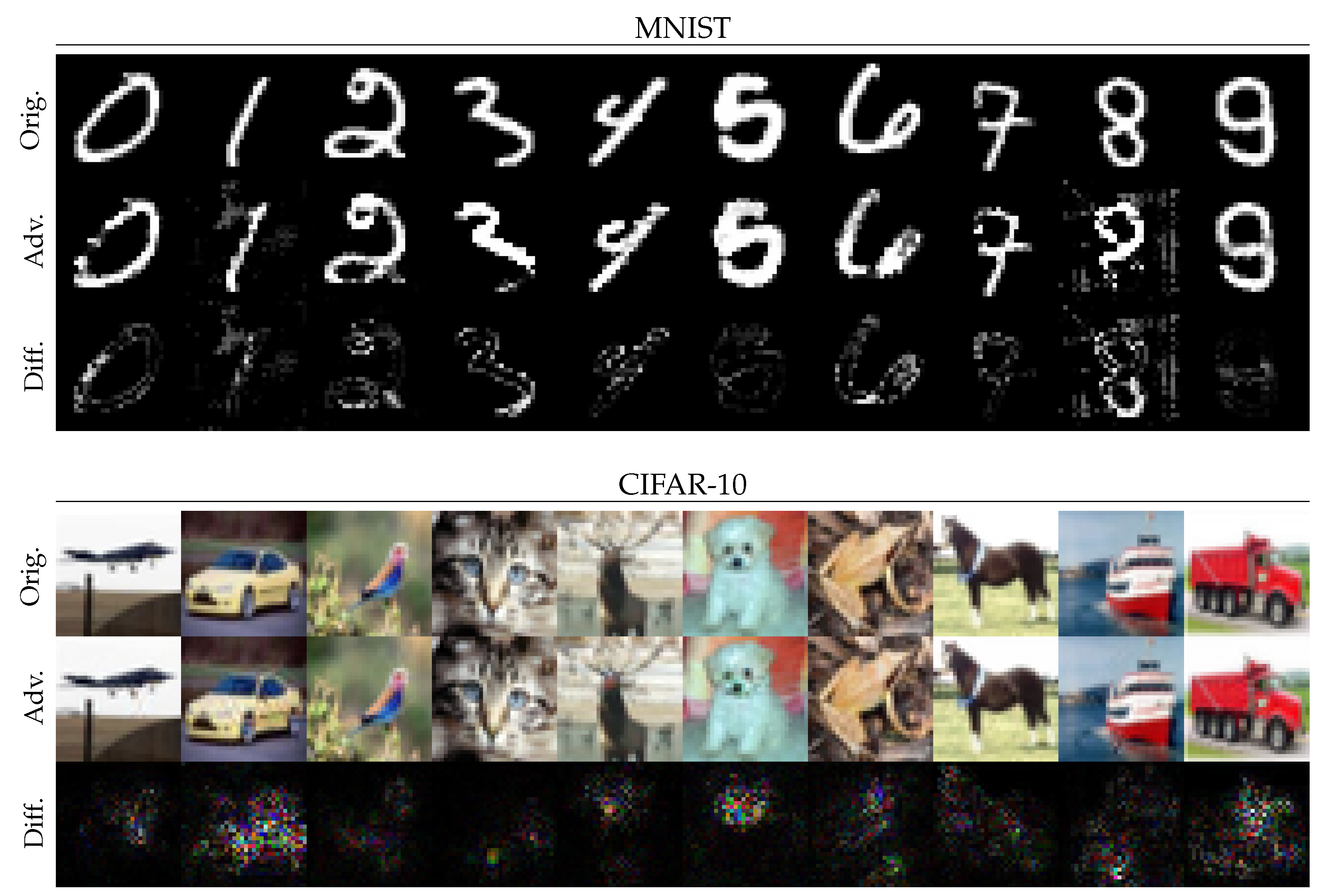
Though ODE-Nets are very promising and perform well, they are vulnerable to the same attacks as the standard networks. However, one of their properties, namely, the ability to change the ODE solver tolerance τ at prediction time, is demonstrated to provide some degree of robustness against basic adversarial attacks [8]. Changing the tolerance value of an adaptive ODE solver causes the solver to adopt different step sizes during the computation of the ODE solution, and this leads to a perturbation of the forward pass that increases the adversarial robustness. Such property is observed even under the CW attack, which represents one of the strongest adversarial algorithms to fool neural networks in image classification specifically. To prove this, a neural ODE model trained on the MNIST and CIFAR-10 datasets, two well-known 10-class image classification benchmarks, has been considered. We used the train split (50k images) of each dataset to train the model and half of the test split (5k images) to generate adversarial samples with the CW attack (examples are reported in Figure 2). The training procedure was performed once with a fixed tolerance value, and we considered multiple values of the tolerance when doing inference and generating adversarial samples.
In Table 1, we report the classification error on the test subset, the attack success rate (in percentage), and the mean L 2 norm of the adversarial perturbation for each tested tolerance value on the two datasets; just for comparison, the results obtained by a standard residual network classifier were inserted. Details on the datasets, models, and adversary generation are available in Section 6. Note that the basic behavior of both the standard residual (RES) and ODE-Net (ODE) models is similar: they show a limited error rate on original images, but on the contrary, the CW attack achieves a very high attack success rate. However, in ODE-Nets, the value of the ODE solver tolerance τ plays an essential role in determining the success rate of an attack; when we increase the value of the tolerance τ used at test time and by the attacker ( τ test = τ attack ), the classification error rate is rather stable, but the required attack budget increases. This is quite clear for the MNIST dataset, where the attack success rate quickly decreases, but it is also appreciable for CIFAR-10 when looking at the mean perturbation introduced by the attack. Though the attack success rate continues to be 100 % , an increasing cost is paid in terms of applied distortion. While this witnesses again to the strength of the CW attack, on the other hand, it confirms that the sensibility to the tolerance variations, found in the case of the projected gradient descent (PGD) attack [8], is also shown by the CW attack, suggesting this being a more general defensive property of ODE-Nets.
Intuition suggests that introducing a decoupling ( τ attack τ test ) between attacker and defender should increase robustness. To verify such hypothesis, we generated adversarial samples by setting a fixed tolerance τ attack and measuring the model’s accuracy when varying the test-time tolerance τ test . By considering a zero-knowledge scenario, the value of attack tolerance τ attack = τ train was taken from the best choice the attacker can make.
At prediction time, the tolerance was drawn from a log-uniform distribution with the interval [ 10 5 , 10 1 ] centered in τ train = 10 3 ; 20 values were sampled for each image to be classified. Figure 3 reports the accuracy of the ODE-Net classifier on original inputs (blue lines) and adversarial examples (orange lines) for MNIST and CIFAR-10 datasets, respectively; the tolerance on the x-axis is binned (21 bins) in the log space.
It is evident that accuracy on natural inputs (blue lines) is always stable and very high for each tolerance value, averagely around the original network accuracy ( 100 % for MNIST and 90 % for CIFAR-10); this means that varying the tolerance does not significantly affect accuracy on standard pristine samples. On the contrary, accuracy on CW-created adversarial inputs (orange lines) is quite poor (this demonstrates the power of such a technique again), but it is very interesting to note that in the central bin (around τ train = 10 3 ) the attack has the highest effectiveness; this seems to mean that when the tolerance at test time coincides with that adopted by the CW attacker, the classifier is strongly induced to misclassify. Furthermore, it can also be appreciated that if τ test is moved away from the central value used by the CW attacker, accuracy increases. This means that changes in the tolerance can provide robustness against CW attack, achieving, for instance, accuracy on adversarial inputs of about 60 % (and corresponding accuracy of around 90 % on original images) for the CIFAR-10 dataset (see Figure 3 on the extreme right). Finally, it is worth observing that the trend of growth of the orange lines is asymmetric with respect to the central value τ train = 10 3 , and higher values were achieved for the right side: this shows, as generally expected, that increasing the tolerance permits one to gain in robustness.

4.1. Defensive Tolerance Randomization

In light of these findings, we exploited tolerance variation as an active measure against adversarial attacks and measured to which extent this defensive property can be effective in an adversarial detection scenario where the defender is asked to discern adversarial samples from authentic ones.
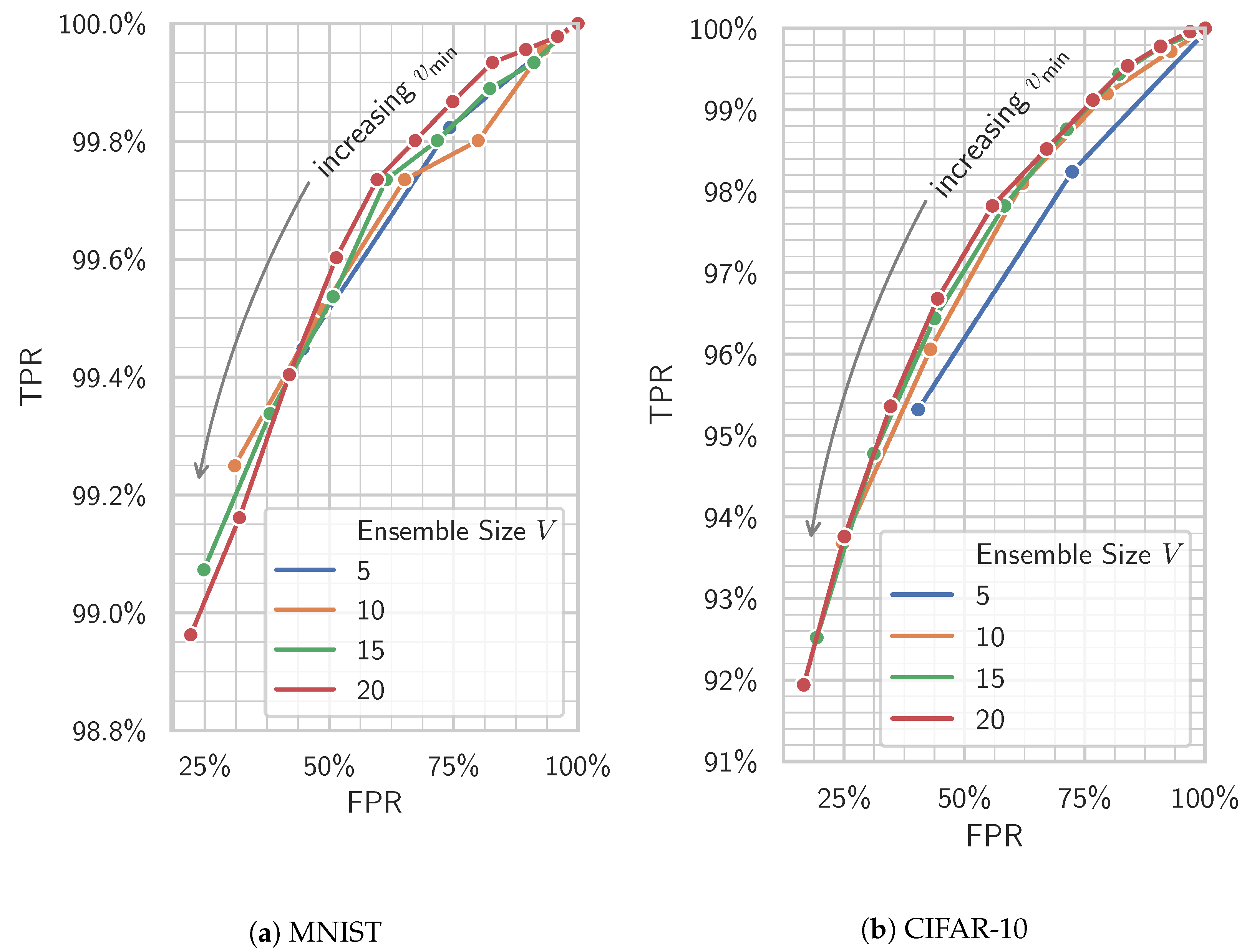
We considered a white-box attack scenario in which the attacker has access to the trained ODE-Net and knows the parameter settings of the classifier—specifically, the solver tolerance τ train used during the network training. An attack is successful if the CW algorithm finds an adversarial perturbation leading to a misclassification without exceeding a prefixed attack budget defined as the maximum number of optimization iterations. According to this, we have introduced an adversarial detection strategy based on ODE-Net, tolerance randomization, which collects several predictions with different randomly drawn test-time tolerance parameters τ test , to detect whether the classification system is subjected to an adversarial sample. τ test is sampled uniformly from a range centered on τ train such that τ train = τ attack τ test . Introducing such a variability also helps the defendant against knowledgeable adversaries, as simply changing τ test to a different fixed value can be easily counteracted by the adversary also changing τ attack to the new value. By indicating with V the number of voting members (i.e., the number of τ values randomly drawn) belonging to the ensemble, we will declare that an adversarial sample is detected if v agree < v min , where v agree is the largest amount of members that have reached the same decision on the test image (size of the majority), and v min is the minimum consensus threshold required for assessing the authenticity (non-maliciousness) of the input.
The performance of this adversarial detection scheme is depicted in Figure 4. We can see that, once establishing the size V of the voting ensemble (different colored lines), by varying the threshold v min with a step of 1, ROC curves can be obtained in terms of TPR versus FPR, where true positive indicates the correct classification of a natural input. Such graphs demonstrate that high TPRs can be registered in correspondence with limited FPRs. This is particularly visible for the MNIST dataset (see Figure 4a), but it is still true for CIFAR-10; if, just for example, we refer to Figure 4b when V = 20 (purple line), by increasing the value of v min (going down along the curve), we can reduce the FPR while maintaining a high TPR: with v min =20 a TPR= 92 % and a corresponding FPR= 15 % are achieved (see the bottom-left corner of Figure 4b). This experiment basically demonstrates that if the ODE-Net is subjected to a zero-knowledge Carlini and Wagner attack in a white-box scenario, by resorting to test-time tolerance randomization, it is possible both to preserve classification performances on natural images and significantly reduce the capacity of the CW attack to fool the ODE classifier at the expense of performing multiple inferences.

5. Robustness under Adaptive Attackers

To date, we have studied tolerance variation for defensive purposes under the assumption of a non-adaptive adversary. In this section, we extend the analysis described in Section 4 and Section 4.1 by also exploring the effect of the attacker’s tolerance when generating adversarial samples.
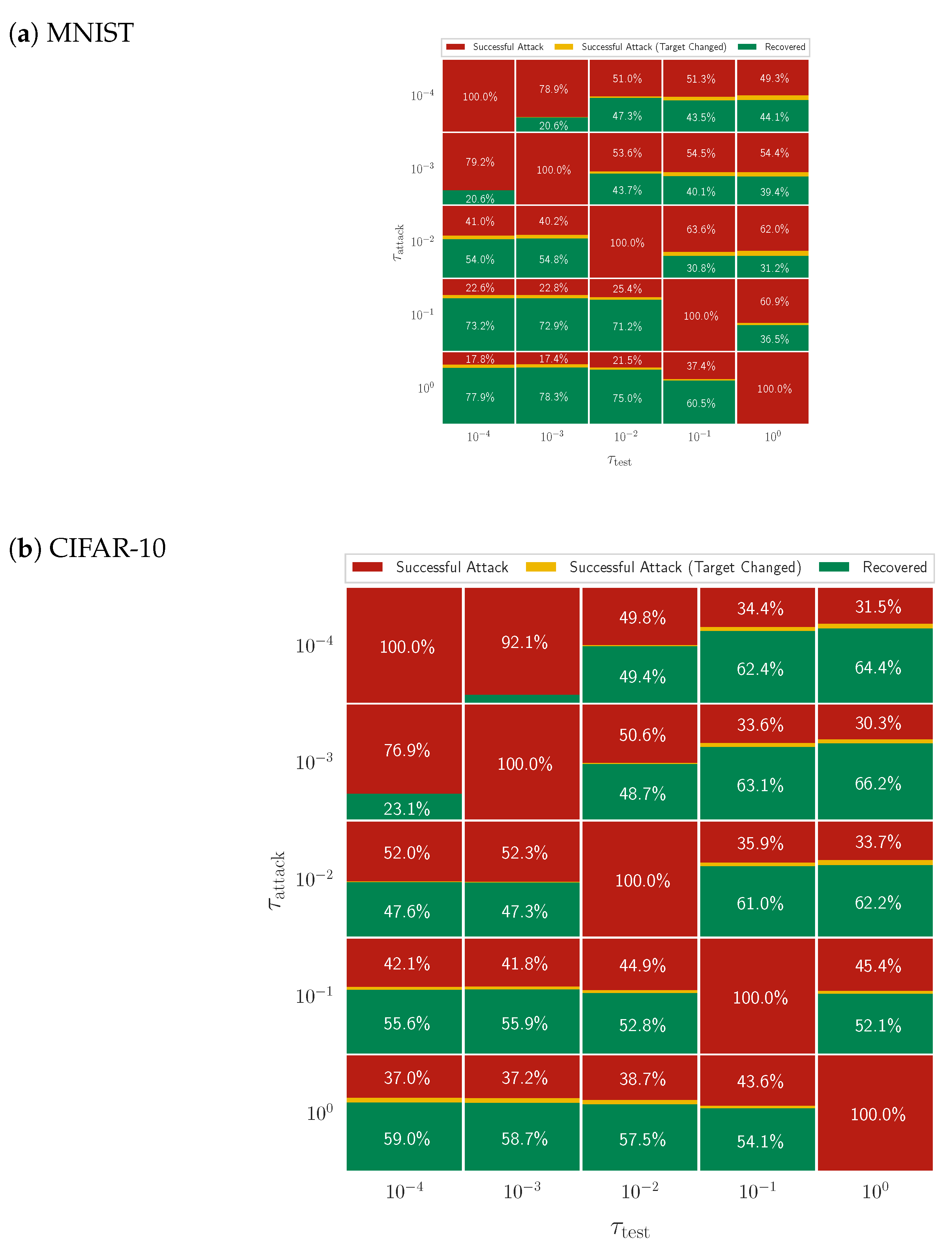
As the defender, the attacker can vary the solver’s tolerance to generate malicious samples. While we observed that the defender should set τ test to a value away from the τ attack , the attacker instead aims at setting τ attack = τ test , where he is certain about the success of the attack. We explored how the CW attack success rate varies over the ( τ attack , τ test ) R 2 space. Instead of a randomized exploration of this space, we performed a logarithmic grid sampling of tolerance values by setting τ = 10 i , i { 4 , 3 , 2 , 1 , 0 } independently for τ attack and τ test . As in previous sections, CW attacks were performed on our trained neural ODE classifiers using the first halves of the MNIST and CIFAR-10 test sets with the solver’s tolerance set to τ attack . We report results in Figure 5, where for each ( τ attack , τ test ) couple, we show the percentage of successful attacks (adversarial samples that fooled the network as intended, in red), the percentage of failed attacks (adversarial samples that were either “recovered” as such or correctly classified by the network, in green), and the percentage of successful but changed attacks (adversarial samples that were still misclassified but were classified differently from what the attacker expected, in yellow). For this experiment, we ignored samples on which the attack failed to generate an adversarial perturbation in the first place, i.e., we discarded samples that failed to generate an adversarial sample when τ attack = τ test , thus having an attack success rate of 100% in the diagonal entries. This permits focusing only on the effect of tolerance decoupling on the attack success rate while discarding the contributions to robustness already studied and presented in Table 1. It is quite evident that tolerance decoupling between attack and defense can be disruptive for an attacker. For instance, this led to an attack failure rate of up to 78.3% for MNIST when ( τ attack , τ test ) = ( 10 0 , 10 3 ) , and 66.2% for CIFAR-10 when ( τ attack , τ test ) = ( 10 3 , 10 0 ) . In general, higher values of recovery tend to be concentrated where the discrepancy between τ attack and τ test is maximum, but this trend seems to saturate as this discrepancy decreases.

6. Experimental Details

This section reports the implementation details of the experiments described in the previous sections of the paper.

6.1. Datasets: MNIST and CIFAR-10

All the models used in this analysis were trained on two standard and well-known image classification benchmarks: MNIST [25] and CIFAR-10 [26]. MNIST is composed of 60,000 grayscale images subdivided into training (50,000) and testing (10,000) sets; images are 28 × 28 pixels and represent hand-written digits (from 0 to 9, so it consists of 10 classes). MNIST is substantially the de fact standard baseline for novel machine learning algorithms and is nearly the only dataset used in research concerning ODE networks. The second dataset taken into account in our analysis was CIFAR-10; it is a 10-class image classification dataset too, comprised of 60,000 RGB images (size 32 × 32 pixels) of common objects subdivided into training/testing sets (50,000/10,000).

6.2. The Training Phase

Both considered models, RES and ODE, apply dropout before the fully-connected classifier with a drop probability of 0.5 , and the SGD optimizer has a momentum of 0.9 ; the weight decay is 10 4 , batch size is 128, and the learning rate is 10 1 reduced by a factor 10 every time the error plateaus. The number of filters K in the internal blocks is differently set for each dataset: 64 for MNIST and 256 for CIFAR-10. For the ODE net model, containing the ODE block, we used the Dormand–Prince variant of the fifth-order Runge–Kutta ODE solver (implemented in https://github.com/rtqichen/torchdiffeq, accessed on 1 August 2022); in such an algorithm, the step size is adaptive and can be controlled by a tolerance parameter τ ( τ train = 10 3 was used in our experiments during the training phase). The value of τ constitutes a threshold for the maximum absolute and relative error (estimated using the difference between the fourth-order and the fifth-order solution) tolerated when performing a step of integration; if such a step error exceeds τ , the integration step is discarded, and the step size decreased. Both models, RES and ODE, the achieved classification performances are comparable with the current state-of-the-art performances on MNIST and CIFAR-10 datasets (see Table 1).

6.3. Carlini and Wagner Attack Implementation Details

The CW attack was implemented by resorting to Foolbox 2.0 [27] on PyTorch models. We adopted Adam to optimize Equation (4), setting the maximum iterations to 100 and performing 5 binary search steps to tune c starting from 10 2 . The learning rate of 0.05 was used for MNIST and 0.01 for CIFAR-10. The first 5000 images of each test set were selected as original samples to be perturbed, discarding the images naturally misclassified by the classifier.

7. Conclusions and Future Works

In this paper, we have presented an analysis of the robustness of neural ODE image classifiers in an uncontrolled environment, and the behavior of N-ODE nets against the Carlini and Wagner (CW) attack was specifically studied. The CW attack was considered, as it is one of the most performing adversarial attacks for the image classification task. Furthermore, we have focused on how the tolerance parameter of the adaptive ODE solver, which is generally used in neural ODE networks to tune the computational precision-efficiency trade-off, can affect the robustness against such attacks. We have observed that modifying the tolerance used during the prediction phase from that used when generating adversarial inputs tends to undermine attacks while maintaining high accuracy on pristine samples. According to this, we have proposed using the tolerance as a defensive property of neural ODE nets and demonstrated that it is possible by introducing a novel adversarial detection strategy for ODE nets based on tolerance randomization and a major voting ensemble scheme.
Our evaluation performed on two standard image classification benchmarks (MNIST and CIFAR-10) has shown that our simple detection technique can reject roughly 80% of strong CW adversarial examples while maintaining +90% of original samples under white-box attacks and zero-knowledge adversaries. We have also hypothesized that to overcome our method, the adversary should require high attack budgets to attack a wide range of tolerance values and distill them in a unique malicious input.
We have also explored the defensive properties of tolerance variation in the scenario with adaptive adversaries and shown that the simple decoupling of attack and test tolerances, without any additional defensive procedures, increases adversarial robustness up to roughly 78% and 66% for MNIST and CIFAR-10 datasets, respectively.
Future works will be dedicated to gathering deeper insights into the relationship between attacker and defender tolerance settings by exploring the tolerance space on a finer scale. In addition, we would be interested to investigate the dynamic scenario in which both the attacker and the defender try to adapt each other and analyze it in a game-theoretic framework.

Author Contributions

Conceptualization, F.C., R.C., F.F. and G.A.; methodology, R.C., F.F. and G.A.; software, F.C.; investigation, F.C. and R.C.; writing—original draft preparation, F.C., R.C. and F.F.; writing—review and editing, F.C., R.C., F.F. and G.A.; supervision, F.F. and G.A. All authors have read and agreed to the published version of the manuscript.

Funding

This work was partially funded by Tuscany POR FSE 2014-2020 AI-MAP (CNR4C program, CUP B15J19001040004), the AI4EU project (EC, H2020, n. 825619) and the AI4Media Project (EC, H2020, n. 951911).

Institutional Review Board Statement

Not applicable.

Informed Consent Statement

Not applicable.

Data Availability Statement

Code and resources to reproduce the experiments presented here are available at https://github.com/fabiocarrara/neural-ode-features/tree/master/adversarial (accessed on 1 August 2022).

Conflicts of Interest

The authors declare no conflict of interest.

References

  1. Szegedy, C.; Zaremba, W.; Sutskever, I.; Bruna, J.; Erhan, D.; Goodfellow, I.J.; Fergus, R. Intriguing properties of neural networks. arXiv 2014, arXiv:1312.6199. [Google Scholar]
  2. Goodfellow, I.J.; Shlens, J.; Szegedy, C. Explaining and Harnessing Adversarial Examples. arXiv 2015, arXiv:1412.6572. [Google Scholar]
  3. Moosavi-Dezfooli, S.M.; Fawzi, A.; Frossard, P. Deepfool: A simple and accurate method to fool deep neural networks. In Proceedings of the IEEE Conference on Computer Vision and Pattern Recognition, Las Vegas, NV, USA, 27–30 June 2016; pp. 2574–2582. [Google Scholar]
  4. Carlini, N.; Wagner, D. Towards evaluating the robustness of neural networks. In Proceedings of the 2017 IEEE Symposium on Security and Privacy (SP), San Jose, CA, USA, 22–26 May 2017; pp. 39–57. [Google Scholar]
  5. Kurakin, A.; Goodfellow, I.J.; Bengio, S. Adversarial Examples in the Physical World; Chapman and Hall: London, UK, 2017. [Google Scholar]
  6. Papernot, N.; McDaniel, P.D.; Wu, X.; Jha, S.; Swami, A. Distillation as a Defense to Adversarial Perturbations Against Deep Neural Networks. In Proceedings of the 2016 IEEE Symposium on Security and Privacy (SP), San Jose, CA, USA, 22–26 May 2016; pp. 582–597. [Google Scholar] [CrossRef] [Green Version]
  7. Wu, J.; Xia, Z.; Feng, X. Improving Adversarial Robustness of CNNs via Maximum Margin. Appl. Sci. 2022, 12, 7927. [Google Scholar] [CrossRef]
  8. Carrara, F.; Caldelli, R.; Falchi, F.; Amato, G. On the robustness to adversarial examples of neural ODE image classifiers. In Proceedings of the 2019 IEEE International Workshop on Information Forensics and Security (WIFS), Delft, The Netherlands, 9–12 December 2019; pp. 1–6. [Google Scholar]
  9. Carrara, F.; Caldelli, R.; Falchi, F.; Amato, G. Defending Neural ODE Image Classifiers from Adversarial Attacks with Tolerance Randomization. In Proceedings of the Pattern Recognition—ICPR International Workshops and Challenges, Virtual Event, 15–20 January 2021; Springer International Publishing: Cham, Switzerland, 2021; pp. 425–438. [Google Scholar]
  10. Papernot, N.; McDaniel, P.; Jha, S.; Fredrikson, M.; Celik, Z.B.; Swami, A. The limitations of deep learning in adversarial settings. In Proceedings of the 2016 IEEE European Symposium on Security and Privacy (EuroS&P), Saarbruecken, Germany, 21–24 March 2016; pp. 372–387. [Google Scholar]
  11. Kurakin, A.; Goodfellow, I.J.; Bengio, S.; Dong, Y.; Liao, F.; Liang, M.; Pang, T.; Zhu, J.; Hu, X.; Xie, C.; et al. Adversarial Attacks and Defences Competition. In The NIPS ’17 Competition: Building Intelligent Systems; Springer: Berlin/Heidelberg, Germany, 2018. [Google Scholar]
  12. Madry, A.; Makelov, A.; Schmidt, L.; Tsipras, D.; Vladu, A. Towards Deep Learning Models Resistant to Adversarial Attacks. arXiv 2018, arXiv:1706.06083. [Google Scholar]
  13. Grosse, K.; Manoharan, P.; Papernot, N.; Backes, M.; McDaniel, P.D. On the (Statistical) Detection of Adversarial Examples. arXiv 2017, arXiv:1702.06280. [Google Scholar]
  14. Metzen, J.H.; Genewein, T.; Fischer, V.; Bischoff, B. On Detecting Adversarial Perturbations. arXiv 2017, arXiv:1702.04267. [Google Scholar]
  15. Carrara, F.; Becarelli, R.; Caldelli, R.; Falchi, F.; Amato, G. Adversarial examples detection in features distance spaces. In Proceedings of the European Conference on Computer Vision (ECCV) Workshops, Munich, Germany, 8–14 September 2018. [Google Scholar]
  16. Taran, O.; Rezaeifar, S.; Holotyak, T.; Voloshynovskiy, S. Defending against adversarial attacks by randomized diversification. In Proceedings of the IEEE/CVF Conference on Computer Vision and Pattern Recognition (CVPR), Long Beach, CA, USA, 15–20 June 2019; pp. 11226–11233. [Google Scholar]
  17. Barni, M.; Nowroozi, E.; Tondi, B.; Zhang, B. Effectiveness of random deep feature selection for securing image manipulation detectors against adversarial examples. In Proceedings of the ICASSP 2020–2020 IEEE International Conference on Acoustics, Speech and Signal Processing (ICASSP), Barcelona, Spain, 4–8 May 2020; pp. 2977–2981. [Google Scholar]
  18. Feinman, R.; Curtin, R.R.; Shintre, S.; Gardner, A.B. Detecting Adversarial Samples from Artifacts. arXiv 2017, arXiv:1703.00410. [Google Scholar]
  19. Carlini, N.; Wagner, D. Adversarial Examples Are Not Easily Detected: Bypassing Ten Detection Methods. In Proceedings of the Proceedings of the 10th ACM Workshop on Artificial Intelligence and Security, Dallas, TX, USA, 3 November 2017; ACM: New York, NY, USA, 2017; pp. 3–14. [Google Scholar] [CrossRef]
  20. Hanshu, Y.; Jiawei, D.; Vincent, T.; Jiashi, F. On robustness of neural ordinary differential equations. arXiv 2019, arXiv:1910.05513. [Google Scholar]
  21. Liu, X.; Xiao, T.; Si, S.; Cao, Q.; Kumar, S.; Hsieh, C.J. Stabilizing Neural ODE Networks with Stochasticity. 2019. Available online: https://openreview.net/forum?id=Skx2iCNFwB (accessed on 1 August 2022).
  22. Chen, T.Q.; Rubanova, Y.; Bettencourt, J.; Duvenaud, D.K. Neural ordinary differential equations. In Advances in Neural Information Processing Systems; MIT Press: Cambridge, MA, USA, 2018; pp. 6572–6583. [Google Scholar]
  23. He, K.; Zhang, X.; Ren, S.; Sun, J. Identity mappings in deep residual networks. In Proceedings of the Computer Vision—ECCV 2016, Amsterdam, The Netherlands, 11–14 October 2016; pp. 630–645. [Google Scholar]
  24. Wu, Y.; He, K. Group normalization. In Proceedings of the European Conference on Computer Vision (ECCV) Workshops, Munich, Germany, 8–14 September 2018; pp. 3–19. [Google Scholar]
  25. LeCun, Y.; Bottou, L.; Bengio, Y.; Haffner, P. Gradient-based learning applied to document recognition. Proc. IEEE 1998, 86, 2278–2324. [Google Scholar] [CrossRef]
  26. Krizhevsky, A.; Hinton, G. Learning Multiple Layers of Features from Tiny Images; Technical Report; University of Toronto: Toronto, ON, Canada, 2009. [Google Scholar]
  27. Rauber, J.; Brendel, W.; Bethge, M. Foolbox: A Python toolbox to benchmark the robustness of machine learning models. arXiv 2017, arXiv:1707.04131. [Google Scholar]
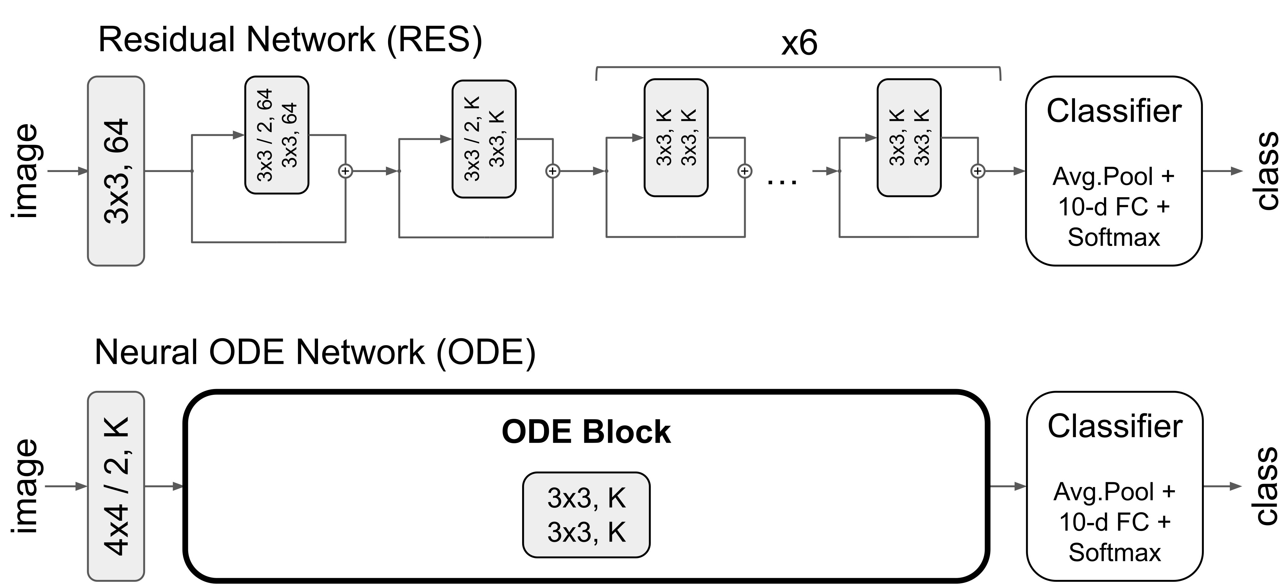
Figure 1. Convolutional layers are written in the format kernel width × kernel height [/ stride], n. filters; padding is always set to 1. For MNIST, K = 64 , and for CIFAR-10, K = 256 .
Information 13 00555 g001
Figure 2. Adversarial examples found with the Carlini and Wagner attack on our neural ODE network on MNIST and CIFAR-10 datasets. Adversarial perturbations (Diff.) of CIFAR-10 samples have been amplified by a factor 10 for visualization purposes.
Information 13 00555 g002
Figure 3. Accuracy vs. test-time solver tolerance τ test . For each image, we sampled 20 values for τ from a log-uniform distribution within the [ 10 5 , 10 1 ] interval. We report the mean accuracy of the ODENet classifier on natural and adversarial examples for each tolerance bin (in log space, points’ x-coordinates indicate the bin centers).
Information 13 00555 g003
Figure 4. Analysis of the detection performance with the randomized tolerance ensemble. ROC curves (TPR vs. FPR, where TP = “correctly detected natural input” and FP = “adversarial input misdetected as natural”) are obtained after varying the minimum majority size v min , i.e., if the number of majoritarian votes v agree in the ensemble is greater than v min , the input is considered authentic (positive), and otherwise, adversarial (negative).
Information 13 00555 g004
Figure 5. Attack success rate (in red) and recovery rate (in green) when varying τ attack (on y-axis) and τ test (on x-axis). In yellow, the percentage of classifications that changed with respect to the one induced by the attack but are still adversarial.
Information 13 00555 g005
Table 1. Classification error (Err, %), Carlini and Wagner attack success rate (ASR, %), and mean L 2 norm perturbation (Pert) of RES and ODE on MNIST and CIFAR-10 test sets; obviously only for ODE are quantities varying the test-time adaptive solver tolerance τ ( τ attack = τ test ) listed.
MNISTCIFAR-10
Err (%)ASR (%)Pert ( × 10 2 )Err (%)ASR (%)Pert ( × 10 5 )
RES0.499.71.17.31002.6
ODE τ = 10 4 0.599.71.49.11002.2
ODE τ = 10 3 0.590.71.79.21002.4
ODE τ = 10 2 0.674.41.99.31004.1
ODE τ = 10 1 0.871.61.710.61008.0
ODE τ = 10 0 1.269.71.911.310013.7
Publisher’s Note: MDPI stays neutral with regard to jurisdictional claims in published maps and institutional affiliations.