2. An LSP Criterion for Water Quality Protection
The decision-making explainability problems are related to specific LSP criterion. To illustrate such problems, we will use the criterion for the Upper Neuse Clean Water Initiative in North Carolina [
7,
8]. The goal is to evaluate specific locations and areas based on their potential for water quality protection. The evaluation team identified 12 attributes that contribute to the potential for water quality protection resulting in the LSP criterion shown in
Figure 1. The stakeholders want to protect undeveloped lands near stream corridors that have soils that can absorb/hold water so that it is possible to avoid erosion and sedimentation and promote groundwater recharge and flood protection.
The aggregation structure in
Figure 1 is based on medium precision aggregators [
1] with three levels (low, medium, high) of hard partial conjunction (HC−, HC, HC+) supporting the annihilator 0, hard partial disjunction (HD−, HD, HD+), supporting the annihilator 1, and soft conjunctive (SC−, SC, SC+) and disjunctive (SD−, SD, SD+) aggregators that do not support annihilators. These are uniform aggregators where the threshold andness is 75% (aggregators with andness or orness above 75% are hard, and aggregators with andness or orness below 75% are soft).
The nodes in the aggregation structure in
Figure 1 are numbered according to the LSP aggregation tree structure where the root node (overall suitability) is the node number 1, and generally, the child nodes of node N are denoted N1, N2, N3, and so on (e.g., the node N = 11 has child nodes 111, 112, 113). In
Figure 1, for simplicity, we also numbered inputs 1, 2, …, 12, so that the input attributes are
and their attribute suitability scores that belong to
are
. The overall suitability is a graded logic function
of attribute suitability scores:
. The details of attribute criteria can be found in [
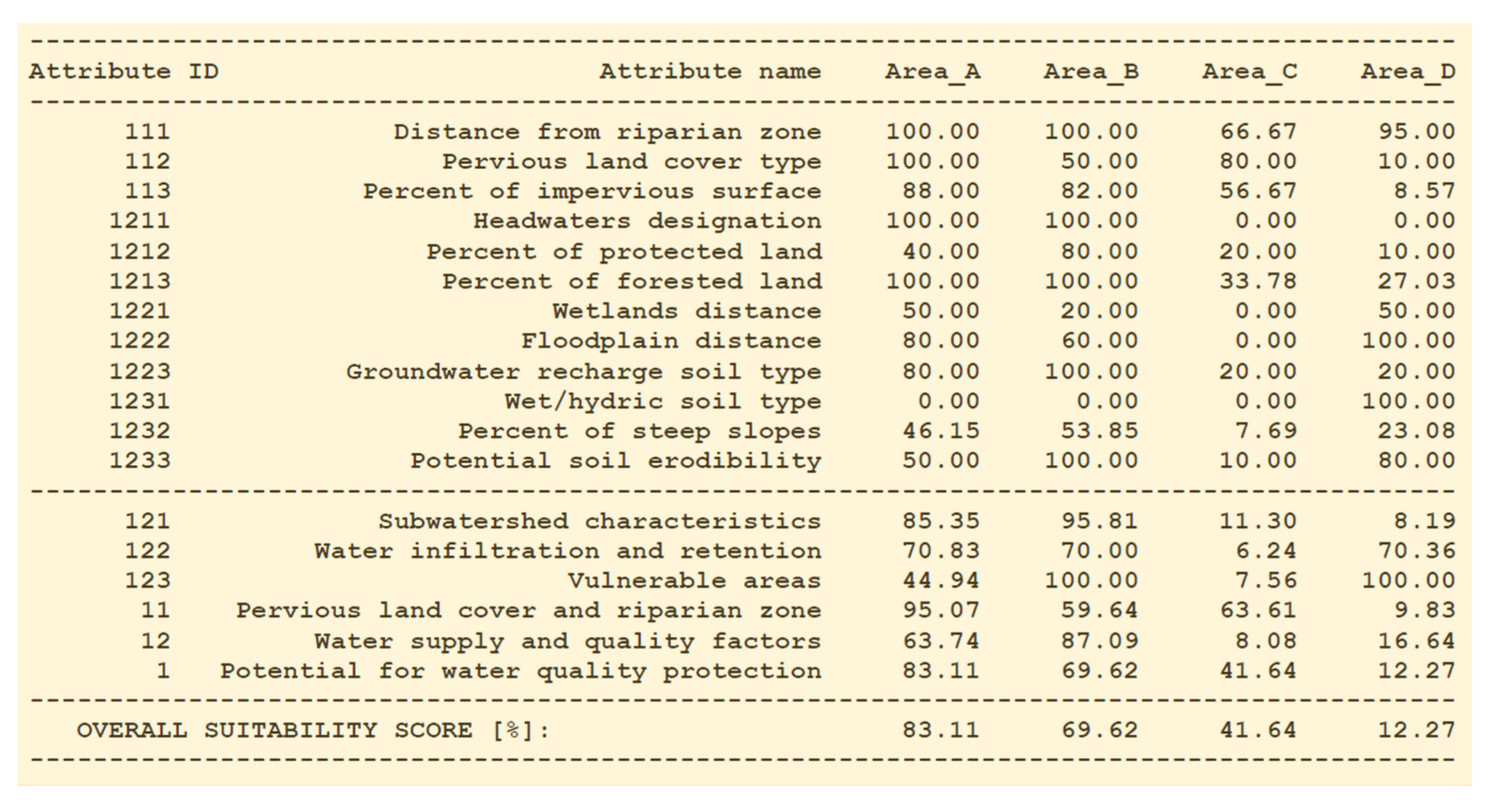
8], and the results of evaluation and comparison of four competitive areas (denoted A, B, C, D), based on the criterion shown in
Figure 1, are presented in
Figure 2.
The point of departure in explaining the properties of the logic aggregation structure is the survey of sensitivity curves
,
, where
c denotes a selected constant; typically,
. The sensitivity curves show the impact of a single input, assuming that all other inputs are constant.
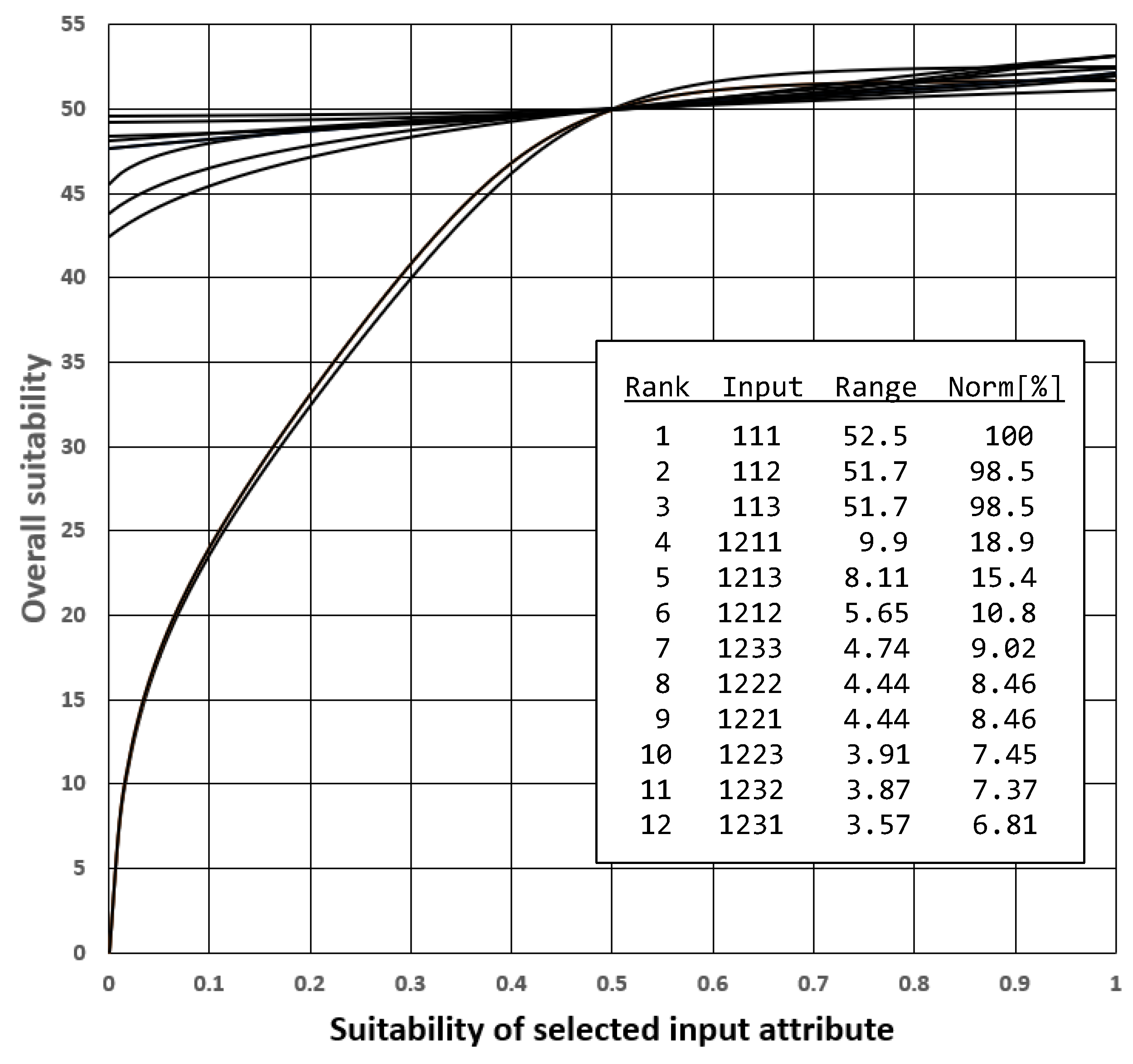
Figure 3 shows the sensitivity curves for the aggregation structure used in
Figure 1, in the case of
.
The relative impact of individual inputs can be estimated using the values of the output suitability range
, and their maximum-normalized values
. These indicators show the change of overall suitability caused by the individual change of selected input attribute suitability in the whole range from 0 to 1. Therefore,
is one of indicators of the
overall impact (or the overall importance) of the given suitability attribute. The corresponding ranking of attributes from the most significant to the least significant should be intuitively acceptable, explainable, and approved by the stakeholder. That is achieved in the ranking shown in
Figure 3 where the first three attributes (111, 112, 113) are mandatory, and all others are optional with different levels of impact. That is consistent with stakeholder requirements specified before the development of the criterion shown in
Figure 1. The normalized values
depend on the value of constant
c, but their values and ranking are rather stable. In
Figure 3 we use
. If
, the ranking of the first six most significant inputs remains unchanged. Minor permutations occur in the bottom six less significant inputs.
The explainability of LSP evaluation project results is a process consisting of the following three main components:
Explainability of the LSP criterion
- 1.1.
Explainability of attributes
- 1.2.
Explainability of elementary attribute criteria
- 1.3.
Explainability of suitability aggregation structure
Explainability of evaluation of individual alternatives
- 2.1.
Analysis of concordance values
- 2.2.
Classification of contributors
Explainability of comparison of competitive alternatives
- 3.1.
Analysis of explainability indicators of individual alternatives
- 3.2.
Analysis of differential effects
The explainability of LSP criterion is defined as a general justification of the validity of criterion (i.e., the consistency between requirements/expectations and the resulting properties of criterion) without considering the available alternatives. In other words, this analysis reflects independent properties of a proposed criterion function. Most actions in the development of an LSP criterion are self-explanatory. The development of a suitability attribute tree is directly based of stakeholder goals, interests, and requirements. The selected suitability attributes should be necessary, sufficient, and nonredundant. Explainability of this step should list reasons why all attributes are necessary and sufficient. In our example, the tree is indirectly visible in
Figure 1. The attribute criteria (shown in [
8]) come with descriptions that for each attribute criterion provide the explanation of reasons for a selected evaluation method. Regarding the suitability aggregation structure (
Figure 1), the only contribution to explainability consists of the sensitivity analysis for constant inputs and for ranking of the overall impact/importance of suitability attributes. All other contributions to explainability are based on specific values of inputs that characterize competitive alternatives.
3. Concordance Values and Explainability of Evaluation Results
In the case of evaluation of a specific object/alternative, each suitability attribute can provide different contributions to the overall suitability
. In the most frequent case of idempotent aggregation structures, we differentiate two groups of input attributes:
high contributors and
low contributors. High contributors are inputs where
; such attribute values are “above the average” and contribute to the increase of the overall suitability. Similarly, low contributors are inputs where
; such attribute values are “below the average” and contribute to the decrease of the overall suitability.
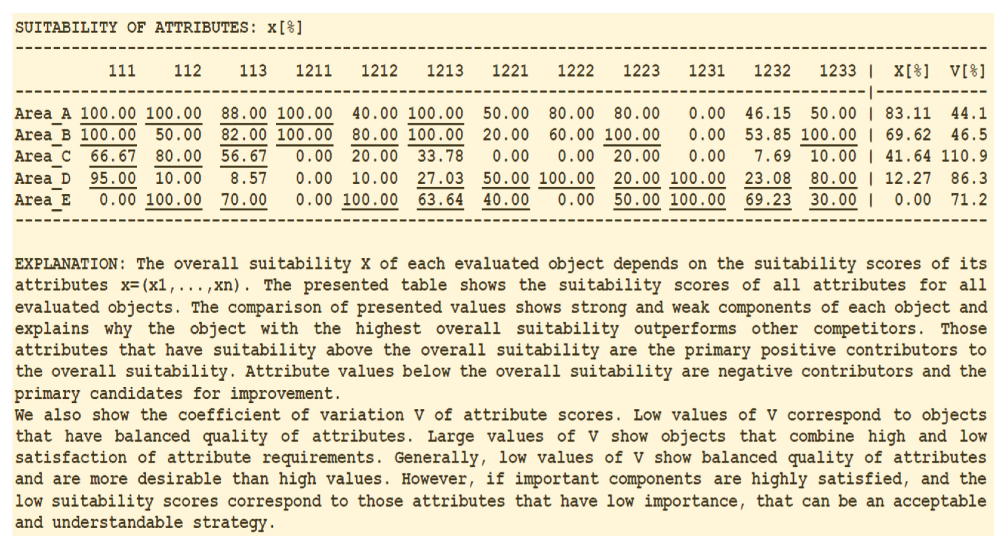
Figure 4 shows the comparison of five areas and all high contributor values are underlined. The overall suitability
shows the resulting ranking of analyzed areas: A > B > C > D > E.
For each attribute, there is obviously a balance point
where the i
th input is in perfect balance with remaining inputs. This value is called the
concordance value and it is crucial for explainability analysis. For all input attributes, the concordance values can be obtained by solving the following equations:
According to the fixed-point iteration concept [
11], these equations can be solved, for each of
attributes, using the following simple convergent numerical procedure:
The concordance values of all attributes for five competitive conservation areas, generated by LSP.XRG, are shown in
Figure 5. Note that the values of all attributes
, are not constants; they are the real values that correspond to the selected competitive area. The concordance value
shows the collective quality of all inputs different from
i. If other inputs are high, then the concordance value of the ith input will also be high, reflecting the general demand for balanced, high satisfaction of inputs. Thus, the concordance values
indicate low contributors, while
characterizes high contributors as shown in
Figure 5 (in all LSP.XRG results the concordance values are denoted
c). According to
Figure 4 and
Figure 5, the Area_E does not satisfy the mandatory requirement 111 (it is too far from the riparian zone) and therefore it is considered unsuitable and rejected by our evaluation criterion. So, the area_E will not be included in subsequent explanations.
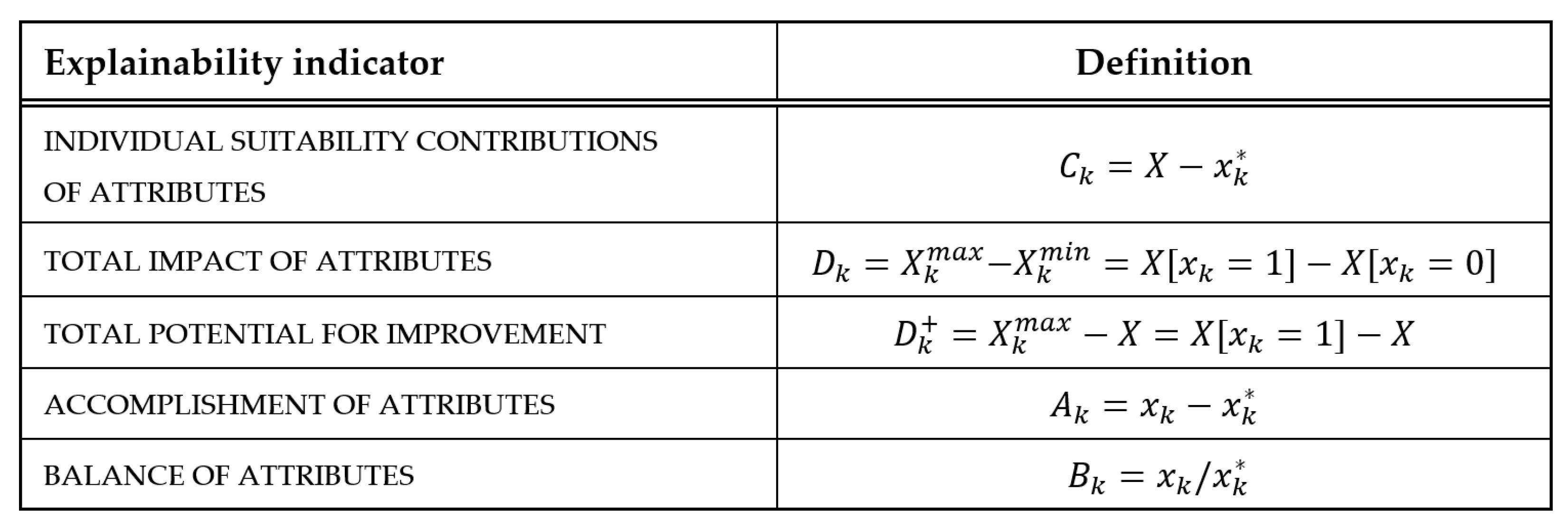
The concordance values are suitable for explaining convenient and inconvenient properties of the specific evaluated area. Indicators that are proposed for explanation are defined in
Figure 6, and then applied and described in detail in
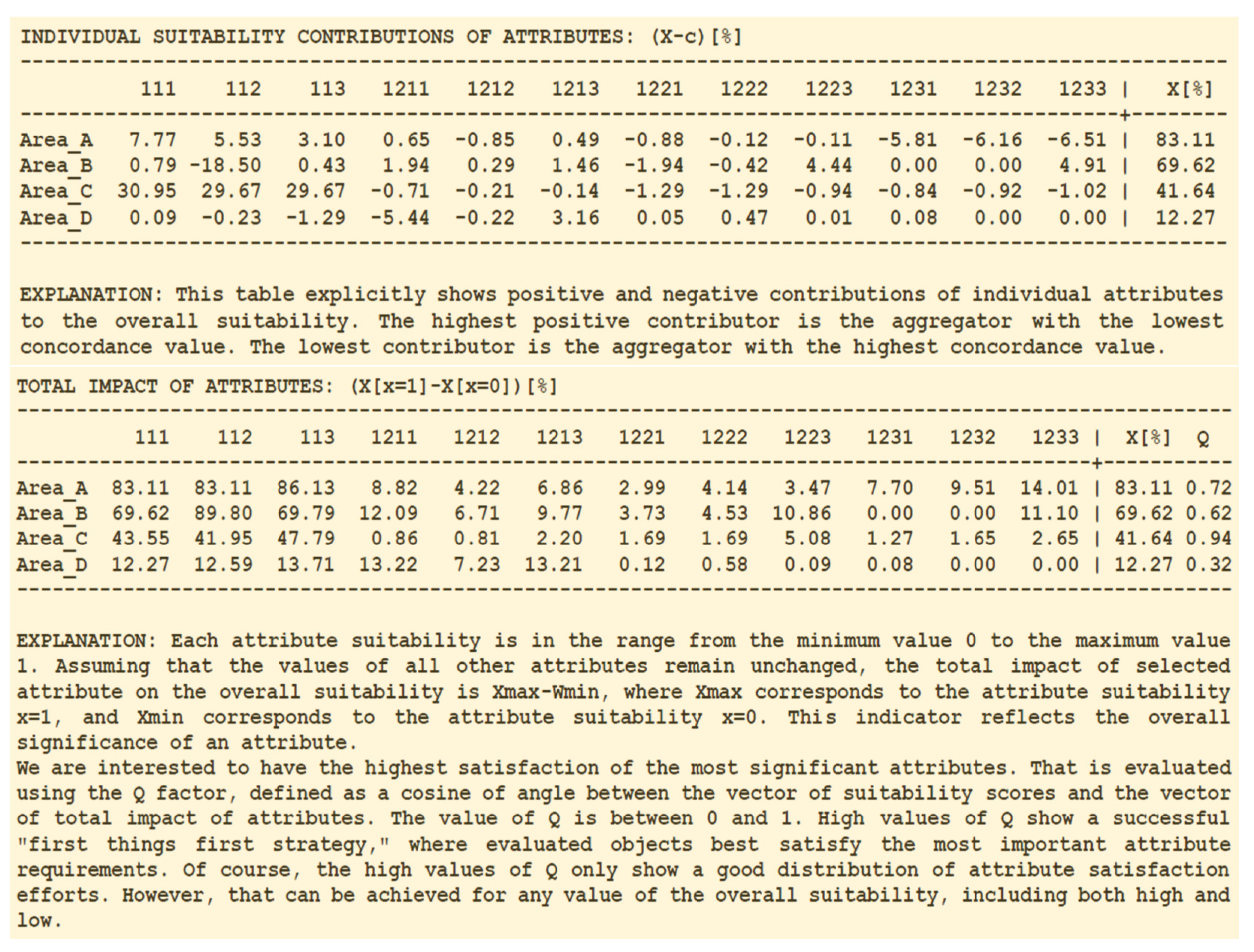
Figure 7. The first question that most stakeholders ask is how individual attributes contribute to the overall suitability X. Since all values
contribute to the value of
X, the most significant individual contributions come from inputs that have the lowest concordance values. Positive contributions shown in the individual contribution table in
Figure 6 correspond to high contributors and negative to low contributors. For example, the primary reason for the highest suitability of the Area_A (with individual contribution of 7.77%) comes from the proximity to riparian zone followed by the convenient pervious land cover type (5.53%) and low percent of impervious surface (3.1%). The individual contributions depend on the structure of the LSP criterion. For example, according to
Figure 4, the Area_A attributes 111, 112, 1211, 1213 have the highest suitability, but their individual contributions are in the range from 0.49% to 7.7%. The negative contributions of Area_A are in vulnerable areas attributes 1231, 1232, 1233 (each of them close to 6%).
The overall impact of individual attributes is an indicator similar to the overall importance of attributes derived from sensitivity curves (defined as the range in
Figure 3). There is a difference: now we analyze the sensitivity of individual attributes based on real values of attributes of each individual alternative (areas A, B, C, D). That offers the possibility for ranking of attributes of individual alternatives according to their impact and (in cases where that is possible) to focus attention on the high impact attributes. However, the high impact is not the same concept as the high potential for improvement.
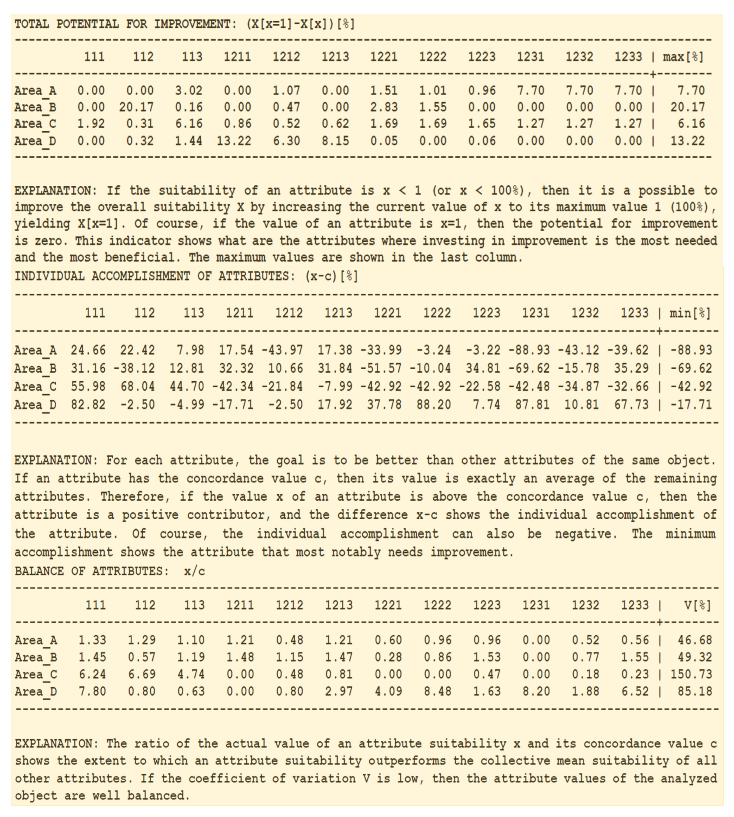
The potential for improvement is defined in
Figure 7 as a real possibility to improve the overall suitability of an alternative. For example, the highest impact attributes of Area_A are already satisfied, and the highest potential for improvement comes from attributes that are insufficiently satisfied. So, the potential for improvement is an indicator that shows (in situations where that is possible) the most impactful attributes that should have the priority in the process of improvement. Their maximum values show the highest potential for improvement of each alternative. Of course, that assumes the possibility of adjustment; unfortunately, physical characteristics of locations and areas cannot be changed.
If an attribute has the value that is significantly above the concordance value, that indicates a high accomplishment, because the quality of that attribute is significantly above the collective quality of other attributes. Exceptionally high accomplishments in a few attributes (e.g., 111, 1222, and 1231 in the case of Area_D) are insufficient to provide high overall suitability and are also an indicator of low suitability of remaining attributes, yielding low ranking of areas D and E (
Figure 4). In the case of Area_E, a single negative accomplishment in a mandatory attribute 111 is sufficient to reject that alternative.
The concordance values offer an opportunity to analyze the balance of attributes. If all attributes are close to their concordance values, that denotes a highly balanced alternative where all attributes have a similar quality. The coefficient of variation (V[%]) of the ratios of actual and concordance values of attributes shows the degree of imbalance and in
Figure 6 the lower quality areas C and D are also significantly imbalanced. Of course, the low imbalance does not mean high suitability; an alternative can have a highly balanced low quality. However, high imbalance generally shows alternatives that need to be improved. Note that the imbalance of attributes in
Figure 7 has the same ranking as the coefficient of variation of the concordance values in
Figure 5; these concepts are similar.
4. Explainability of the Comparison of Alternatives
Explainability of evaluation results contributes to understanding the results of ranking of individual alternatives. However, stakeholders are regularly interested in explaining the specific reasons why an alternative is superior/inferior compared to another alternative. Consequently, the comparison of alternatives needs explanations focused on discriminative properties of LSP criteria.
The superiority of the leading alternative in an evaluation project is a collective effect of all inputs and it cannot be attributed to a single attribute. However, an estimate of individual effects can be based on the direct comparison of the suitability degrees of individual attributes. Suppose that the Area_A has the attribute suitability degrees
, and the Area_B has the attribute suitability degrees
. Then, according to
Figure 4, we have
and
. An estimate of the individual effect of attribute
, compared to the same attribute in the Area_B, can be obtained using the discriminators of attributes
Similarly,
The discriminator shows the individual contribution of selected attribute to the ranking A > B. If then the selected attribute positively contributes to the ranking A > B; similarly, if , then the selected attribute negatively contributes to the ranking A > B. If , then there is no contribution of the selected attribute. We use n discriminators for all n attributes to explain the individual attribute contributions to the ranking of two objects/alternatives. This insight can significantly contribute to explainability reports.
If
, then
positively contributes to the ranking A > B, and to condition
(i.e., their signs are different). Since the discriminators
show the superiority of attributes of the Area_A with respect to the attributes of the Area_B, and
shows the superiority of attributes of the Area_B with respect to the attributes of the Area_A, it follows that these are two different views of the same relationship between two alternatives. To consider both views, we can average them and compute the
mean superiority of the Area_A with respect to the Area_B for specific attributes as follows:
An overall indicator of superiority can be now defined as a “mean overall superiority”
The pairwise comparison of areas A, B, C, D is shown in
Figure 8. The first three rows contain the comparison of areas A and B. The first row contains discriminators
, and the second row contains discriminators
. The mean superiority
is computed in the third row. The rightmost column shows the overall suitability scores of competitive objects (
and
), followed by the mean overall superiority of the first object,
It should be noted that the individual attribute superiority indicators
are useful for comparison of objects, and discovering critical issues, but they do not take into account the difference in importance between attributes. So,
shows unweighted superiority which is different from the difference in the overall suitability. Thus, we can investigate the values of the indicator
. In our examples that value is rather stable (from 10.42 to 17.25), but not constant. This result shows that the overall indicator of superiority
is a useful auxiliary indicator for estimation of relationships between two competitive objects. The main contribution of discriminators to explainability is that they clarify the aggregator-based origins of dominance of one object with respect to another object.
From the standpoint of explainability of the comparison of objects, the individual indicators
explicitly show the predominant strengths (as high positive values) and predominant weaknesses (as low negative values) of the specific object. For example, in
Figure 8, the main advantage of the Area_A compared to the Area_B is the attribute 112 (pervious land cover) and the main disadvantage is attribute 1233 (potential soil erodibility). Such relationships are useful for summarized verbal explanations of a proposed decision that the protection of Area_A should have priority with respect to the protection of Area_B).
In cases where that is possible, the explicit visibility of disadvantages and weaknesses is useful for explaining what properties should be improved, and in what order. Of course, some evaluated objects (e.g. computer systems, cars, airplanes, etc.) have the possibility to modify suitability attributes in order to increase their overall suitability. In such cases, the explainability indicators such as the potential for improvement, the individual suitability contributions, and the individual superiority scores, provide the guidelines for selecting the most effective corrective actions. In the case of locations and areas that are suitable for the water quality protection, the suitability attributes are physical properties that cannot be modified by decision-makers. In such cases the resulting potential for water quality protection cannot be changed, but the ranking of areas and explainability indicators are indispensable to make correct and trustworthy decisions about various protection and development activities.

