
Prediction of Tomato Yield in Chinese-Style Solar Greenhouses Based on Wavelet Neural Networks and Genetic Algorithms


Abstract
:1. Introduction
- (1)
- In this paper, a basic model of yield prediction was applied to describe the non-linear relationship between tomato yield and environmental factors and eight variables are selected as input parameters for the yield predictive model. However, the parameters cannot accurately acquire in the basic model of yield prediction. Therefore, the accuracy of the basic model of yield prediction is difficult to meet actual needs.
- (2)
- To the best of the author’s knowledge, the GA-WNN model has not been used for tomato yield forecasting so far. This model takes advantage of the automatic search ability and probability optimization ability in the global space of the genetic algorithm. In this paper, GA optimizes the dilation and translation factor, thresholds, and the initial weight of the wavelet neural network. Then, in the prediction of tomato yield, this model can obtain the optimal network dilation factor, translation factor and weight. The accuracy of the models was reflected by the MRE, RMSE, EC, the predicted average and the predicted standard deviation. The results of the simulations show that the GA-WNN model is more robust and offers a better function approximation ability, which is useful from theoretical and technical perspectives for quantitative tomato yield prediction in CSGs.
2. Materials
3. Basic Model of Yield Prediction
4. Methodology
4.1. BP Neural Network
4.2. Wavelet Neural Network
4.3. GA-WNN
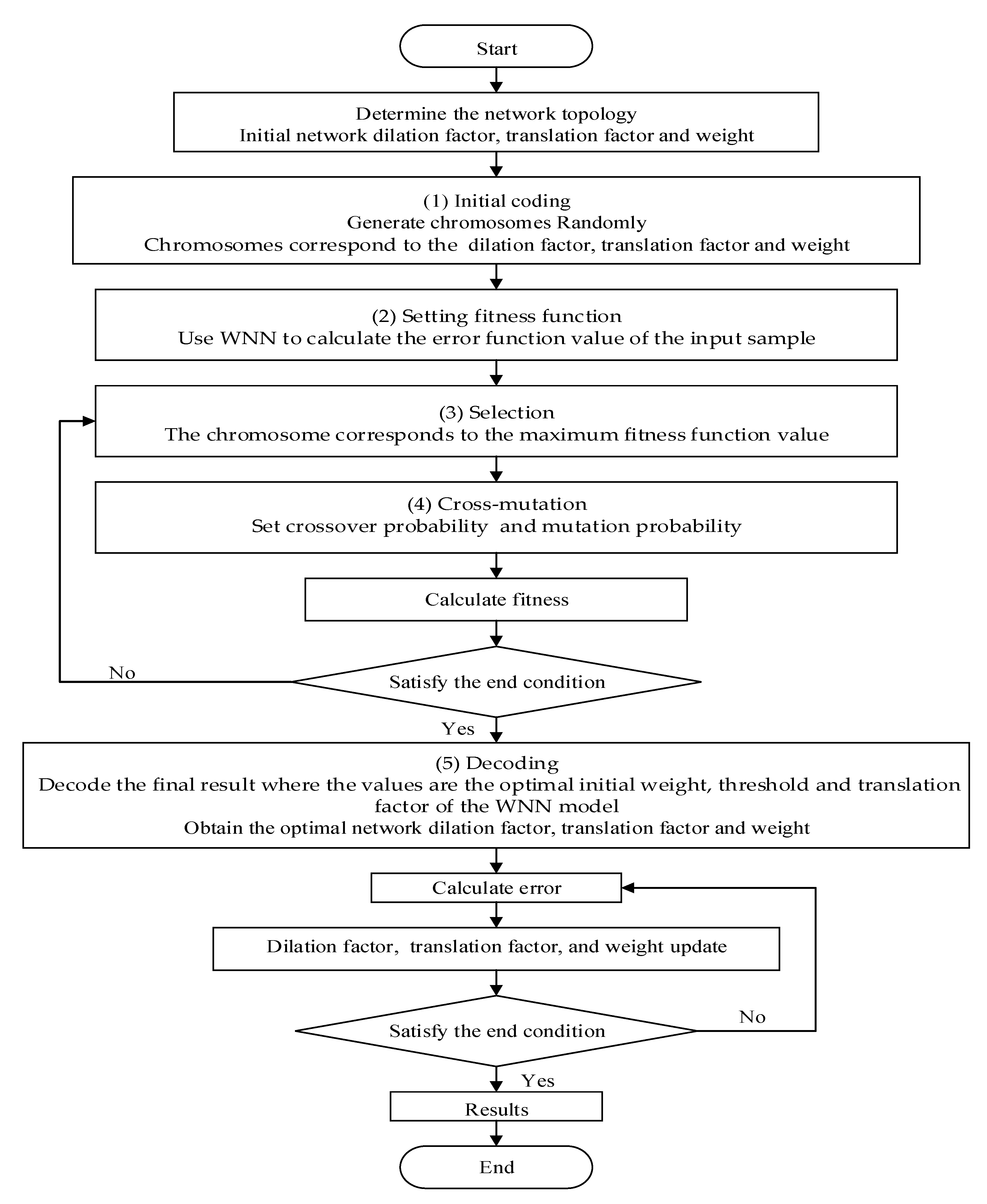
- (1)
- Coding: Firstly, groups of chromosomes are generated randomly. Secondly, these chromosomes correspond to the dilation and translation factor, the connection weight, and the neuron threshold of the wavelet neural network. Thirdly, the crossover and mutation probability are initialized, respectively. Subsequently, the initial population number and the total genetic algebra are given in advance, respectively.
- (2)
- Setting fitness function: Use a wavelet neural network to calculate the error function value of the input sample. Calculate the fitness value of the chromosome corresponding to the reciprocal of the error. Then, sequence the fitness value respectively.
- (3)
- Selection: The formula for calculating the cumulative selection probability of the chromosome is . is a random ascending sequence in the interval of 0–1, When , the chromosome corresponds to the maximum fitness function value. Then, inherit this value directly to the next generation.
- (4)
- Cross-mutation: Set crossover probability and mutation probability . If the performance of the training data is not good, we should return the selection process.
- (5)
- Decoding: Decode the final result where the values are the optimal initial weight, threshold and translation factor of the wavelet neural network prediction model.
5. Results and Analysis
5.1. Evaluation Parameters
5.2. Collection and Processing of Historical Data
- (1)
- During the measurement of the ambient parameter data, it should be noted that some data may exceed normal values or not match the current environmental conditions due to the improper use of measuring instruments or incorrect sensor settings. Incorrect data should be eliminated and new data should be used via linear interpolation instead of the incorrect data.
- (2)
- In order to ensure model prediction accuracy and function convergence speed, the data need to be normalized to finally obtain input data for the prediction model [26,27]. A linear function conversion method was used to normalize the data (Equation (19)):where is the measured value of the instrument, and are the maximum and minimum values of the same parameter data, and is the normalized value. Through the above formula, the data were normalized to values within the range of 0–1. In this way, the dynamic range of the data was reduced and the model prediction accuracy was improved.
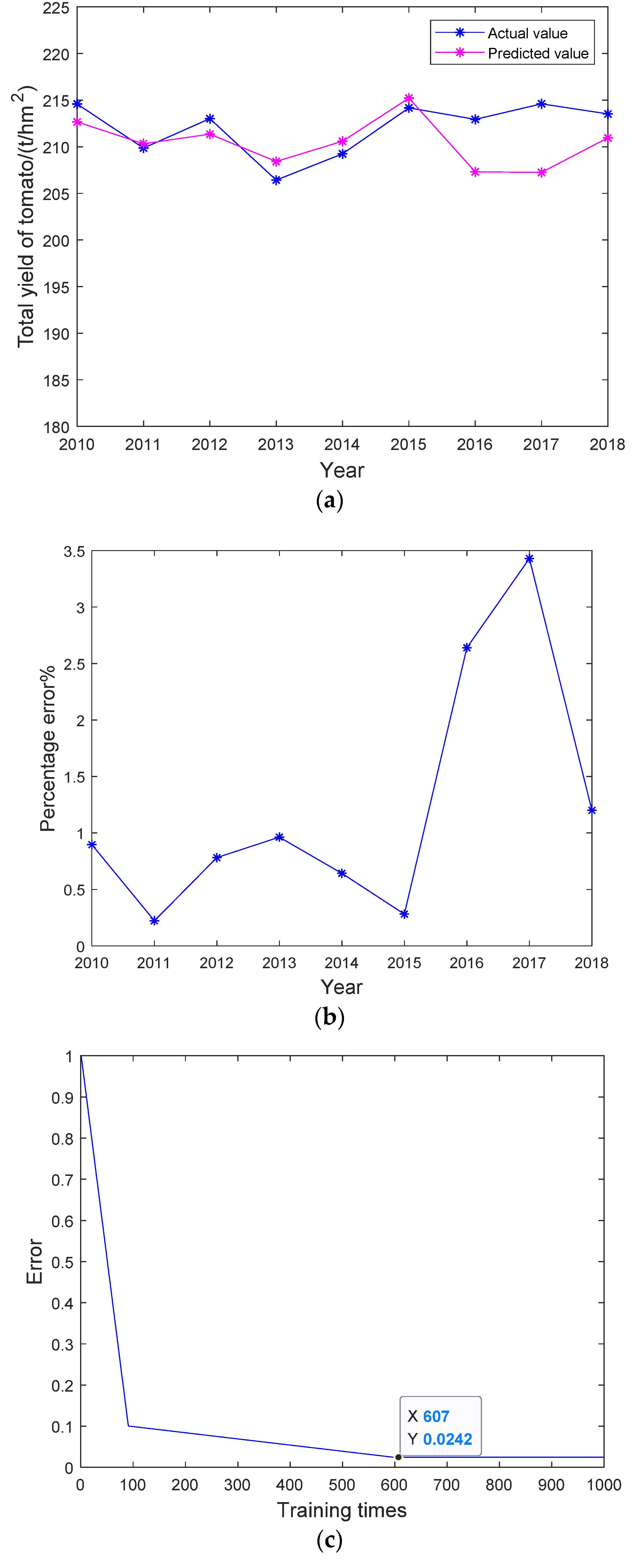
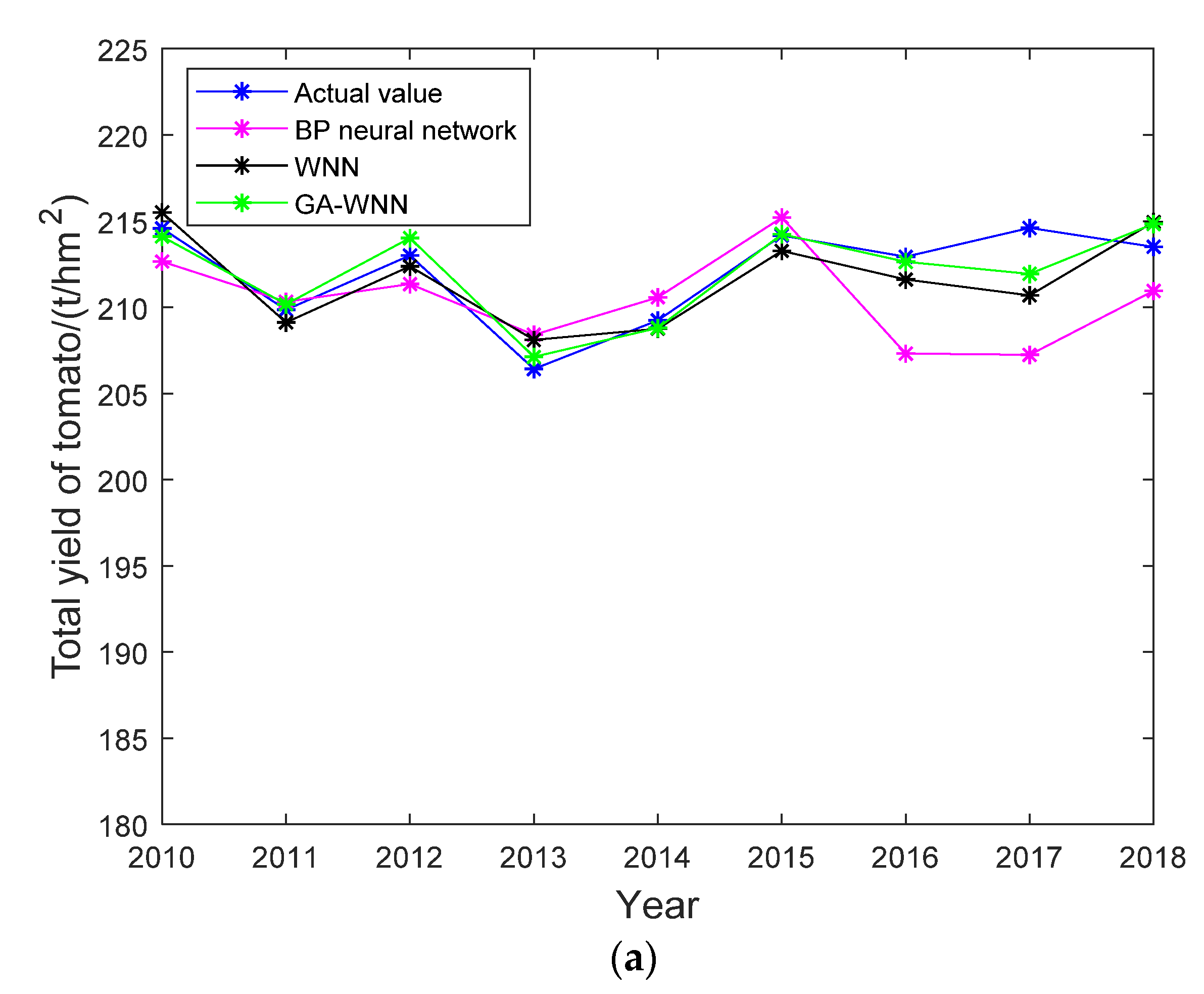
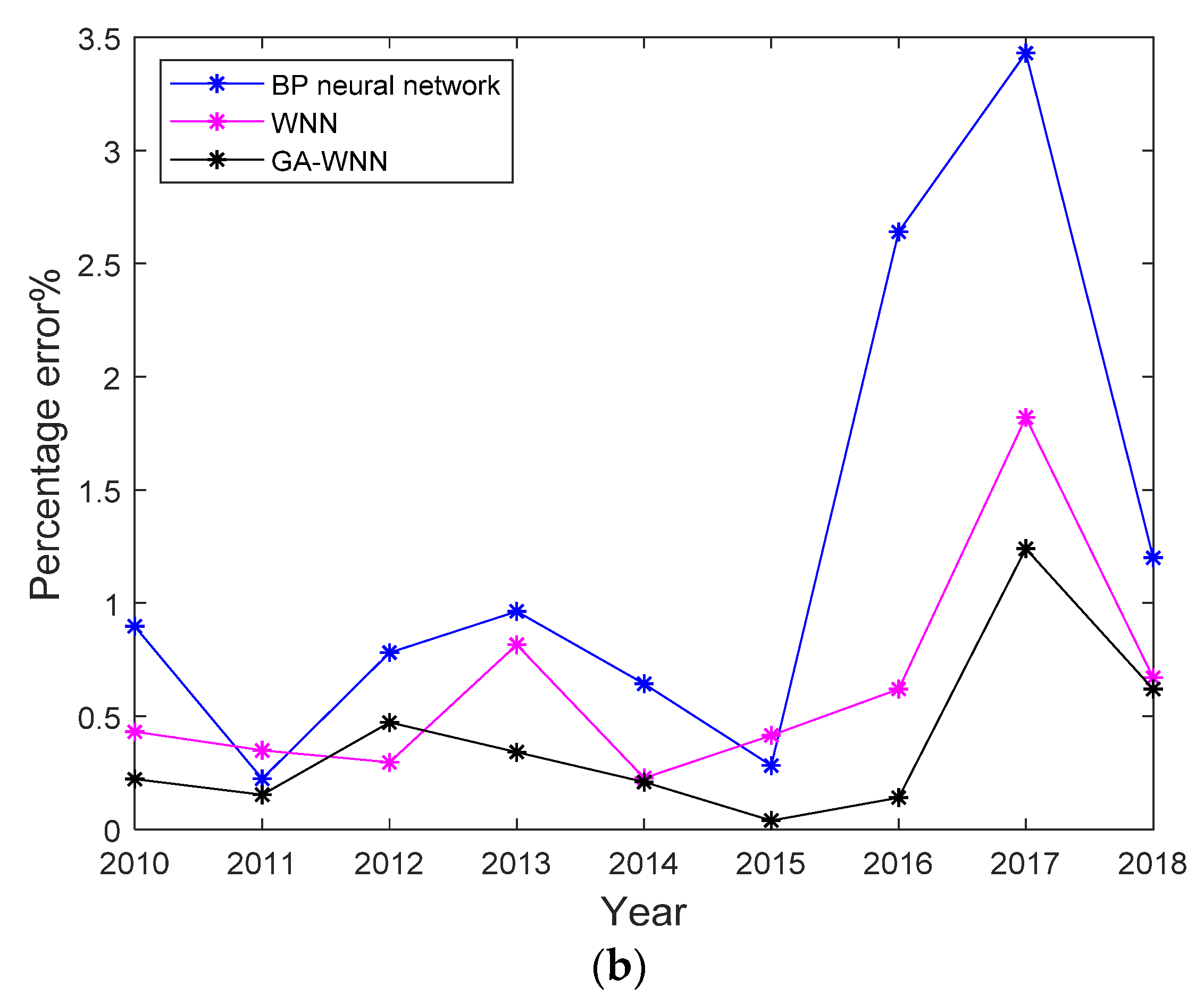
5.3. Analysis of BP Neural Network Model and Results
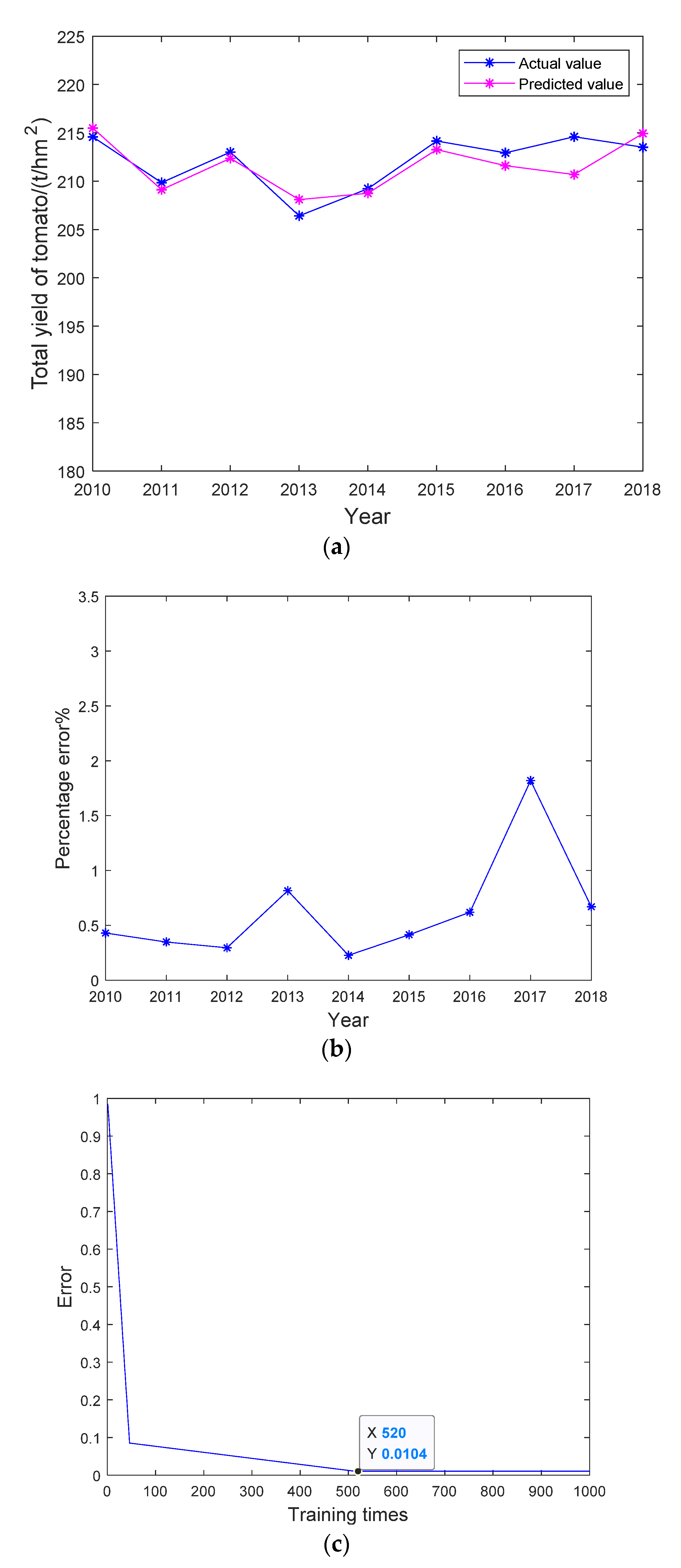
5.4. Analysis of the WNN Model and Results
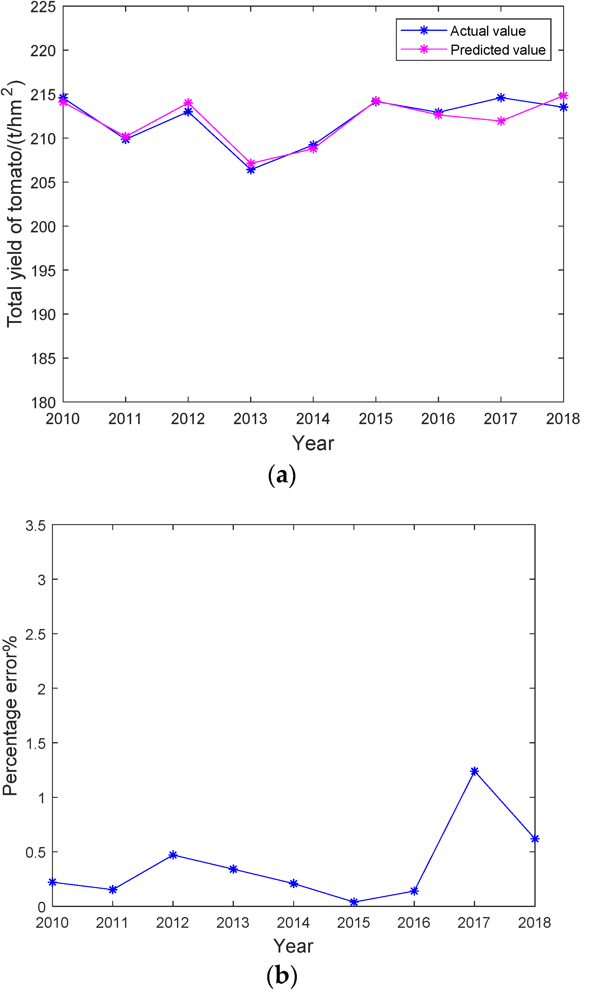
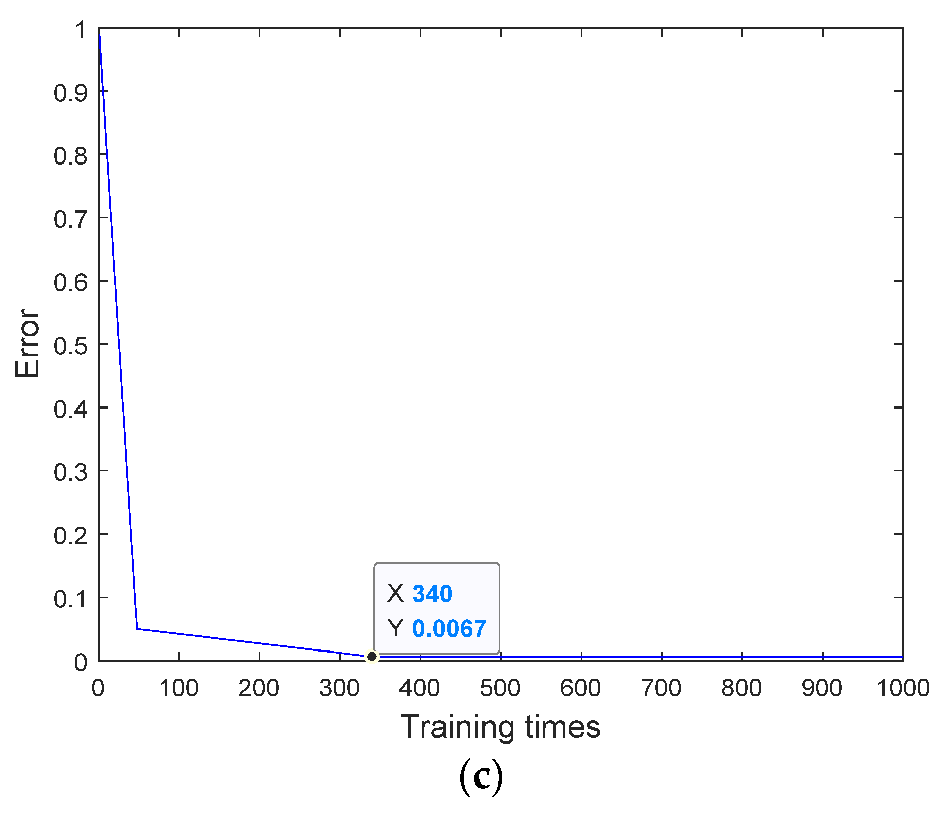
5.5. Analysis of the GA-WNN Model and Results
6. Discussion
7. Conclusions
Author Contributions
Funding
Institutional Review Board Statement
Informed Consent Statement
Data Availability Statement
Acknowledgments
Conflicts of Interest
References
- Leoni, C. Focus on lycopene. Acta Hort. 2003, 797, 25–36. [Google Scholar] [CrossRef]
- FAO. Statistical Database. Available online: http://faostat3.fao.org/home/E (accessed on 10 February 2016).
- Meirelles, G.; Manzi, D.; Brentan, B.; Goulart, T.; Luvizotto, E.J. Calibration Model for Water Distribution Network Using Pressures Estimated by Artificial Neural Networks. Water Resour. Manag. 2017, 31, 4339–4351. [Google Scholar]
- Shabani, A.; Ghaffary, K.A.; Sepaskhah, A.R.; Kamgar-Haghighi, A.A. Using the artificial neural network to estimate leaf area. Sci. Hortic. 2017, 216, 103–110. [Google Scholar]
- López-Aguilar, K.; Benavides-Mendoza, A.; González-Morales, S.; Juárez-Maldonado, A.; Chiñas-Sánchez, P.; Morelos-Moreno, A. Artificial Neural Network Modeling of Greenhouse Tomato Yield and Aerial Dry Matter. Agriculture 2020, 10, 97. [Google Scholar]
- Rohani, A.; Abbaspourfard, M.H.; Abdolahpour, S. Prediction of tractor repair and maintenance costs using Artificial Neural Network. Expert Syst. Appl. 2011, 38, 8999–9007. [Google Scholar]
- Salazar, R.; Dannehl, D.; Schmidt, U.; López, I.; Rojano, A. A dynamic artificial neural network for tomato yield prediction. Acta Hortic. 2017, 1154, 83–90. [Google Scholar]
- Gholipoor, M.; Nadali, F. Fruit yield prediction of pepper using artificial neural network. Sci. Hortic. 2019, 250, 249–253. [Google Scholar] [CrossRef]
- Hu, Z.F.; Zhang, L.D.; Wang, Y.X.; Shamaila, Z.; Zeng, A.J.; Song, J.L.; Liu, Y.J.; Wolfram, S.; Joachim, M.; He, X.K. Application of BP Neural Network in Predicting Winter Wheat Yield Based on Thermography Technology. Spectrosc. Spectr. Anal. 2013, 33, 1587–1592. [Google Scholar]
- Yin, G.H.; Gu, J.; Liu, Z.X.; Hao, L.; Tong, N. Analysis of Grain Yield Prediction Model in Liaoning Province. In Advances in Future Computer and Control Systems; Jin, D., Lin, S., Eds.; Springer: Berlin, Germany, 2012; Volume 159, pp. 355–360. [Google Scholar]
- Zhang, J.Q.; Zhang, W.B.; He, Y.T.; Yan, Y. Predicting the amount of coke deposition on catalyst pellets through image analysis and soft computing. Meas. Sci. Technol. 2016, 27, 114006. [Google Scholar]
- Lu, Z.J.; Zhu, L.; Pei, H.P. The model of chlorophyll-a concentration forecast in the West Lake based on wavelet analysis and BP neural networks. Acta Ecol. Sin. 2008, 28, 4965–4973. [Google Scholar]
- Fang, J.; Zhang, Z. Prediction of human blood pressure based on wavelet analysis and BP neural network. Comput. Syst. Appl. 2017, 26, 157–161. [Google Scholar]
- Li, S.X.; Yao, C.A.; Wen, J.; Huang, X.; Shao, X.H. Forecasting of Basin Sediment Yield Based on Wavelet-BP Neural Network. In Proceedings of the International Asia Conference on Informatics in Control, Automation and Robotics (CAR), Wuhan, China, 6–7 March 2010; pp. 96–99. [Google Scholar]
- Yd, A.; Zfa, B.; Yp, A.; Yz, A.; Hy, A.; Xla, B. Precision fertilization method of field crops based on the wavelet-bp neural network in China. J. Clean. Prod. 2019, 246, 118735. [Google Scholar]
- Yang, X.H.; Liu, X.P.; Liu, H.S.; Guo, Y.; Xu, S.P. Research based on the neural network of simulated annealing and genetic algorithm in the precise fertilization. Guangdong Agric. Sci. 2012, 39, 60–69. [Google Scholar]
- Peng, Y.N.; Xiang, W.L. Short-term traffic volume prediction using GA-BP based on wavelet denoising and phase space reconstruction. Phys. A Stat. Mech. Its Appl. 2020, 549, 14. [Google Scholar] [CrossRef]
- Shen, X.Y.; Zhang, F.; Lv, H.T.; Liu, J.; Liu, H.X. Prediction of Entering Percentage into Expressway Service Areas Based on Wavelet Neural Networks and Genetic Algorithms. IEEE Access 2019, 7, 54562–54574. [Google Scholar] [CrossRef]
- Zhang, D.P.; Zhang, T.Y.; Ji, J.W. Estimation of Solar Radiation for Tomato Water Requirement Calculation in Chinese-Style Solar Greenhouses Based on Least Mean Squares Filter. Sensors 2019, 20, 155. [Google Scholar] [CrossRef] [PubMed] [Green Version]
- Tong, G.; Christopher, D.M.; Li, B. Numerical modelling of temperature variations in a Chinese solar greenhouse. Comput. Electron. Agric. 2009, 68, 129–139. [Google Scholar] [CrossRef]
- Chen, X.L.; Zhang, X.F.; Luo, X.L.; Liu, J.G.; Yao, Y.S. Study of dynamic simulation model of maize growth in northeast China. J. Jilin Agric. Univ. 2012, 34, 242–247. [Google Scholar]
- Yang, Y.; Wang, J.; Weng, H.; Hou, J.; Gao, T. Research on Online Correction of SOC Estimation for Power Battery Based on Neural Network. In Proceedings of the IEEE Advanced Information Technology, Electronic and Automation Control Conference, Xi’an, China, 12–14 October 2018. [Google Scholar]
- Zhang, J. Wavelet neural network for function learning. IEEE Trans. Signal Process. 1995, 43, 1485–1497. [Google Scholar] [CrossRef]
- Chaves, P.; Chang, F.J. Intelligent reservoir operation system based on evolving artificial neural networks. Adv. Water Resour. 2008, 31, 926–936. [Google Scholar] [CrossRef]
- Ouyang, L.; Zhu, F.; Xiong, G.; Zhao, H.; Wang, F.; Liu, T. Short-Term Traffic Flow Forecasting Based on Wavelet Transform and Neural Network. In Proceedings of the 2017 IEEE 20th International Conference on Intelligent Transportation Systems (ITSC), Yokohama, Japan, 16–19 October 2017. [Google Scholar]
- Guo, Z.X.; Wong, W.K.; Li, M. Sparsely connected neural network-based time series forecasting. Inf. Sci. 2012, 193, 54–71. [Google Scholar] [CrossRef]
- Wong, W.K.; Guo, Z.X.; Leung, S.Y.S. Partially connected feedforward neural networks on apollonian networks. Phys. A Stat. Mech. Its Appl. 2010, 389, 5298–5307. [Google Scholar] [CrossRef]

| Nitrogen (g/kg) | Phosphorus (g/kg) | Potassium (g/kg) | Available Phosphorus (mg/kg) | Available Potassium (mg/kg) | Available Nitrogen (mg/kg) | Organic Matter Content (g/kg) |
|---|---|---|---|---|---|---|
| 0.87 | 1.58 | 20.78 | 35.20 | 48.94 | 97.55 | 13.73 |
| Year | Ambient Temperature (°C) | Ambient Humidity (RH%) | Irrigation × 103 (m3·hm−2) | Nitrogen Fertilizer × 102 (kg·hm−2) | Phosphate Fertilizer × 102 (kg·hm−2) | Potassium Fertilizer × 102/(kg·hm−2) | CO2 Concentration × 103 (ppm) | Light Intensity × 104 (lx) | Total Tomato Yield (t·hm−2) |
|---|---|---|---|---|---|---|---|---|---|
| 2010 | 21.83 | 72.95 | 2.11 | 4.05 | 1.89 | 1.96 | 1.01 | 2.54 | 214.578 |
| 2011 | 22.61 | 71.27 | 2.08 | 3.64 | 1.90 | 1.98 | 0.99 | 2.49 | 209.853 |
| 2012 | 25.61 | 74.93 | 2.00 | 3.87 | 1.97 | 1.92 | 1.32 | 2.58 | 213.005 |
| 2013 | 22.97 | 71.92 | 2.08 | 3.79 | 1.98 | 1.83 | 1.30 | 2.30 | 206.417 |
| 2014 | 24.96 | 72.61 | 2.10 | 3.45 | 1.82 | 1.86 | 1.27 | 2.23 | 209.231 |
| 2015 | 21.98 | 70.46 | 2.07 | 3.70 | 1.83 | 1.81 | 1.19 | 2.41 | 214.159 |
| 2016 | 22.52 | 72.17 | 2.04 | 3.87 | 1.88 | 1.87 | 0.94 | 2.65 | 212.929 |
| 2017 | 23.58 | 74.65 | 2.07 | 4.04 | 1.81 | 1.92 | 1.38 | 2.47 | 214.598 |
| 2018 | 24.72 | 73.79 | 2.06 | 3.68 | 1.91 | 1.98 | 1.06 | 2.32 | 213.508 |
| Learning Rate | Momentum Coefficient | Maximum Allowable Error | Number of Hidden Layer Nodes | Prediction Error (%) |
|---|---|---|---|---|
| 0.09 | 0.85 | 0.01 | 3 | 5.08 |
| 0.09 | 0.85 | 0.01 | 4 | 3.86 |
| 0.09 | 0.85 | 0.01 | 5 | 2.42 |
| 0.09 | 0.85 | 0.01 | 6 | 2.93 |
| 0.09 | 0.85 | 0.01 | 7 | 3.82 |
| 0.09 | 0.85 | 0.01 | 8 | 4.45 |
| Learning Rate | Momentum Coefficient | Maximum Allowable Error | Number of Hidden Layer Nodes | Prediction Error (%) |
|---|---|---|---|---|
| 0.09 | 0.85 | 0.01 | 3 | 4.12 |
| 0.09 | 0.85 | 0.01 | 4 | 2.86 |
| 0.09 | 0.85 | 0.01 | 5 | 1.31 |
| 0.09 | 0.85 | 0.01 | 6 | 1.04 |
| 0.09 | 0.85 | 0.01 | 7 | 2.53 |
| 0.09 | 0.85 | 0.01 | 8 | 3.40 |
| Prediction Method | Mean Relative Error | Root Mean Square Error | EC | Convergent Iterations |
|---|---|---|---|---|
| BP neural network | 0.0242 | 5.548 | 0.9868 | 607 |
| WNN | 0.0104 | 2.520 | 0.9935 | 520 |
| GA-WNN | 0.0067 | 1.725 | 0.9960 | 340 |
Publisher’s Note: MDPI stays neutral with regard to jurisdictional claims in published maps and institutional affiliations. |
© 2021 by the authors. Licensee MDPI, Basel, Switzerland. This article is an open access article distributed under the terms and conditions of the Creative Commons Attribution (CC BY) license (https://creativecommons.org/licenses/by/4.0/).
Share and Cite
Wang, Y.; Xiao, R.; Yin, Y.; Liu, T. Prediction of Tomato Yield in Chinese-Style Solar Greenhouses Based on Wavelet Neural Networks and Genetic Algorithms. Information 2021, 12, 336. https://doi.org/10.3390/info12080336
Wang Y, Xiao R, Yin Y, Liu T. Prediction of Tomato Yield in Chinese-Style Solar Greenhouses Based on Wavelet Neural Networks and Genetic Algorithms. Information. 2021; 12(8):336. https://doi.org/10.3390/info12080336
Chicago/Turabian StyleWang, Yonggang, Ruimin Xiao, Yizhi Yin, and Tan Liu. 2021. "Prediction of Tomato Yield in Chinese-Style Solar Greenhouses Based on Wavelet Neural Networks and Genetic Algorithms" Information 12, no. 8: 336. https://doi.org/10.3390/info12080336
APA StyleWang, Y., Xiao, R., Yin, Y., & Liu, T. (2021). Prediction of Tomato Yield in Chinese-Style Solar Greenhouses Based on Wavelet Neural Networks and Genetic Algorithms. Information, 12(8), 336. https://doi.org/10.3390/info12080336