Article

Adaptive Multi-Scale Wavelet Neural Network for Time Series Classification

College of Electronic Science and Technology, National University of Defense Technology, Changsha 410073, China
*
Author to whom correspondence should be addressed.
Information 2021, 12(6), 252; https://doi.org/10.3390/info12060252
Submission received: 16 May 2021 / Revised: 12 June 2021 / Accepted: 14 June 2021 / Published: 17 June 2021
(This article belongs to the Section Artificial Intelligence)

Abstract

:
Wavelet transform is a well-known multi-resolution tool to analyze the time series in the time-frequency domain. Wavelet basis is diverse but predefined by manual without taking the data into the consideration. Hence, it is a great challenge to select an appropriate wavelet basis to separate the low and high frequency components for the task on the hand. Inspired by the lifting scheme in the second-generation wavelet, the updater and predictor are learned directly from the time series to separate the low and high frequency components of the time series. An adaptive multi-scale wavelet neural network (AMSW-NN) is proposed for time series classification in this paper. First, candidate frequency decompositions are obtained by a multi-scale convolutional neural network in conjunction with a depthwise convolutional neural network. Then, a selector is used to choose the optimal frequency decomposition from the candidates. At last, the optimal frequency decomposition is fed to a classification network to predict the label. A comprehensive experiment is performed on the UCR archive. The results demonstrate that, compared with the classical wavelet transform, AMSW-NN could improve the performance based on different classification networks.

1. Introduction

In recent years, the research on time series classification has achieved unprecedented prosperity [1]. Time series data from the accelerometers, gyroscopes, or magnetic field sensors is used to recognize the human activity recognition [2]. Data recorded by the electroencephalogram (EEG) is important to help the doctor to study brain function and neurological disorders [3]. Mid-infrared spectroscopy analysis is also useful to discriminate the freshness of food [4]. To better compare different researches for time series classification, UCR archive [5] is built and there are at least one thousand published papers making use of at least one dataset from this archive.
The methods for time series classification can be divided into two categories:time-domain methods and frequency-domain methods [6]. Time-domain methods such as shapelets [7] and elastic distance measures [8] consider the shape of time series is important to the classification. Compared with the time-domain methods, frequency-domain methods such as Bag-of-SFA-Symbols [9] and Word Extraction for Time Series Classification [10] predict the label of the time series by analyzing the spectrum.
In the last few years, with the development of deep learning, the process of time series classification has been further advanced. Convolutional Neural Network (CNN) such as Fully Convolutional Network (FCN) and Residual Network [11] achieve the competitive performance with traditional methods. Recently, an Inception network suitable for time series called Inceptiontime [12] is proposed and achieves the state-of-the-art performance on the UCR archive. Most of the published methods learn discriminative features directly from the time domain. There are some attempts to combine the frequency representation of the time series with deep learning [5,13]. Wavelet transform is a widely used time-frequency analysis tool that has superior time-frequency localization as compared with the Discrete Fourier Transform and Short Time Fourier Transform [14]. Wavelet transform decomposes the time series into low and high frequency components by the wavelet basis. A variety of the wavelet bases such as Harr, Morlet, and Daubechies have been proposed. Despite the remarkable achievement of the wavelet transform, there is still room for improvement. In the classical wavelet transform, the wavelet basis is artificially predefined which could be inappropriate for the task on the hand. To overcome this limitation, the second-generation wavelet emerged [15]. A lifting scheme is proposed to extract the low and high frequency components from the time series adaptively.
Inspired by the lifting scheme, an adaptive multi-scale wavelet neural network (AMSW-NN) is proposed in this paper. Instead of separating the low and high frequency components by the predefined polynomials, a multi-scale combined with a depthwise CNN is used in the AMSW-NN to obtain the candidate frequency decompositions, an optimal frequency decomposition is selected from the candidates. The primary contributions of this paper are concluded as follows:
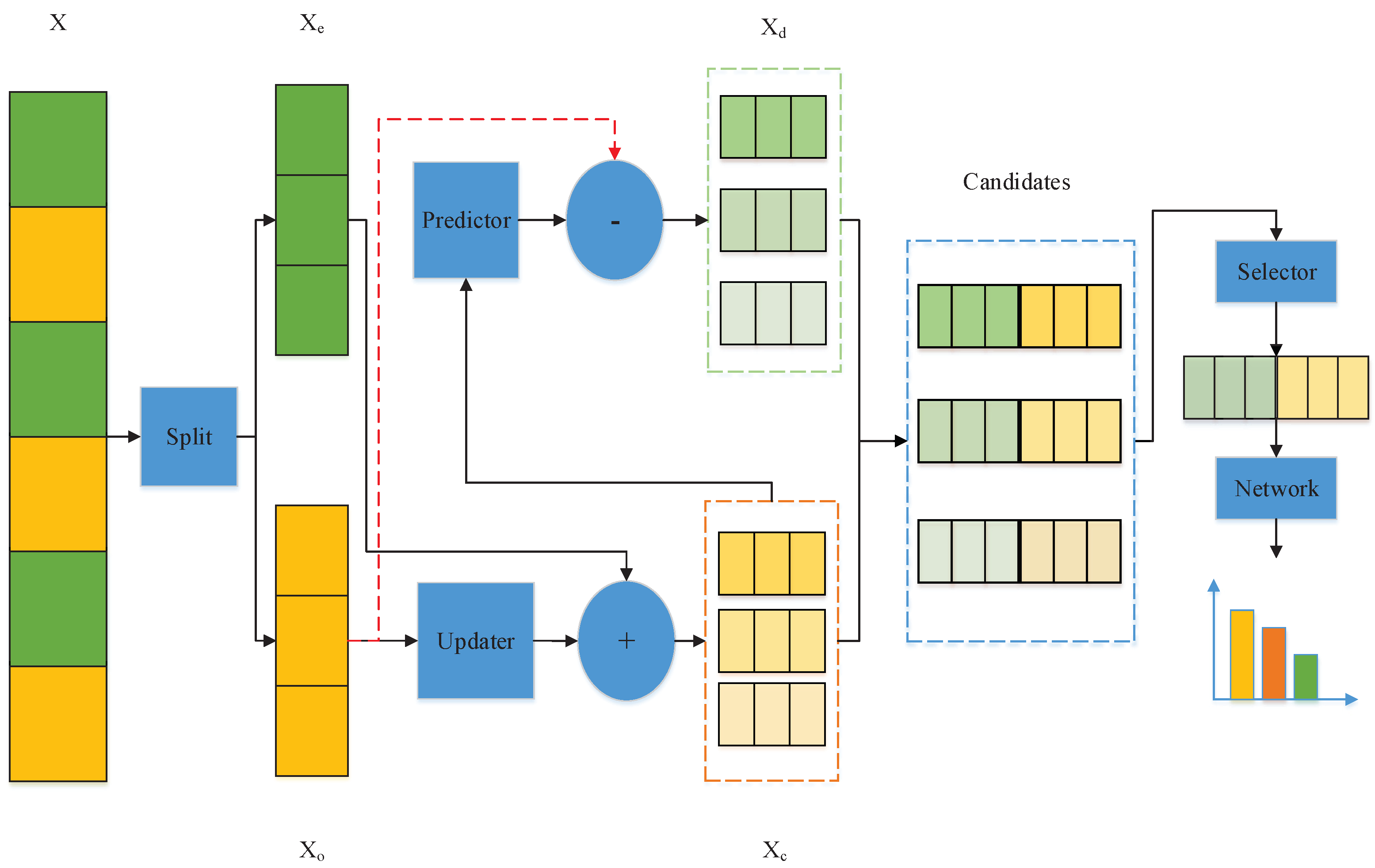
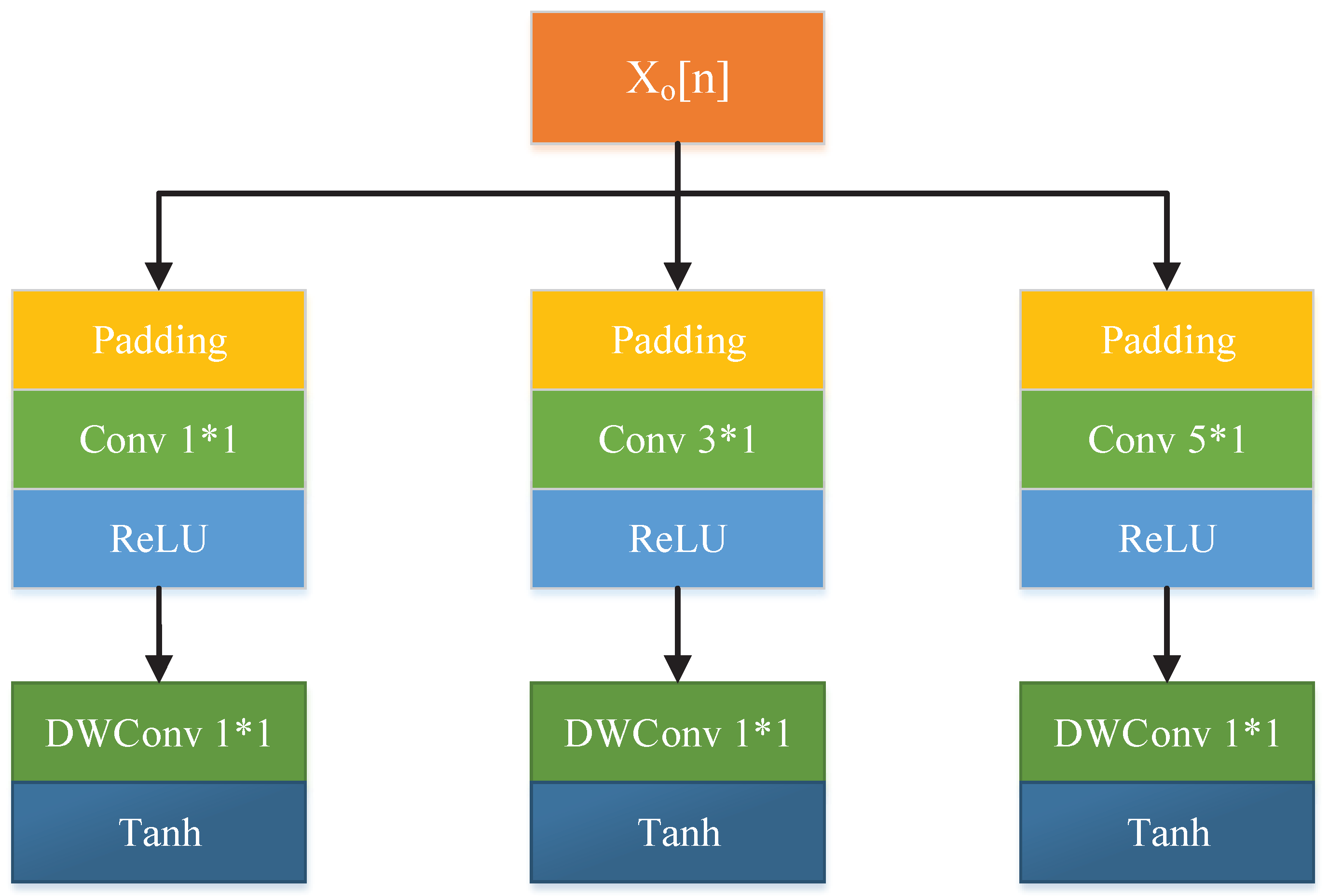
  • A multi-scale combined with a depthwise CNN is proposed to learn the candidate frequency decompositions of the time series.
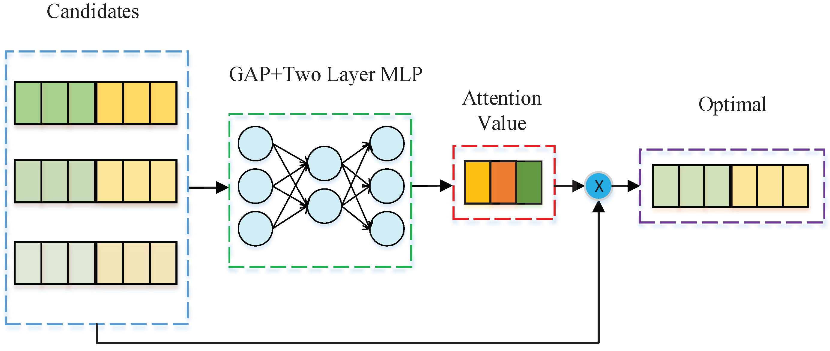
  • The optimal frequency decomposition is selected from the candidates by a selector.
  • The experiments performed on the UCR archive [5] demonstrate that the AMSW-NN could achieve a better performance based on different classification networks compared with the classical wavelet transform.
The remainder of this paper is organized as follows. Background is reviewed in Section 2. In Section 3, AMSW-NN is proposed to extract the low and high frequency components from the time series. Next, the extensive experiments are performed on the UCR archive, and the results and discussions are presented in Section 4. Finally, a conclusion is provided in Section 5.

2. Background

This section briefly introduces the lifting scheme in the second-generation wavelet which is the building block of the proposed method.

2.1. Lifting Scheme

The second-generation wavelet is known as the lifting wavelet [16]. Compared with the classical wavelet (also called the first-generation wavelet), the lifting wavelet does not rely on the Fourier transform. Hence, a lifting scheme could be applied in the situation where the Fourier transform is unavailable [17]. The lifting scheme is usually divided into three steps including split, prediction, and update. The order of prediction and update can be reversed. The update-first structure is used in the proposed method due to the stability [18] and described in this section.
The overall flowchart of the lifting scheme is shown in Figure 1. A time series X = ( x 1 , x 2 , , x N ) is split into the even component X e and odd component X o as presented in Equation (1):
X e [ n ] = X [ 2 k 1 ] , X o [ n ] = X [ 2 k ] ,
where k = 1 , 2 n / 2 .
After the split, the information contained in the time series X is decomposed into the even component X e and odd component X o . The low frequency component X c of the time series X is approximated by the running average as shown in Equation (2):
X c [ n ] = X e [ n ] + U ( X o [ n ] ) ,
where U ( ) is an update filter.
When the low frequency component X c is obtained, the high frequency component X d could be predicted by the X c and X o as presented in Equation (3):
X d [ n ] = X o [ n ] P ( X c [ n ] ) ,
where P ( ) is a prediction filter.

2.2. Adaptive Lifting Scheme

The predictor and updater in the original lifting scheme are constructed by the predefined polynomials which is a suboptimal solution. Consider the excellent mapping and self-learning ability of the Back Propagation (BP) network. The predictor and updater in the adaptive lifting scheme are constructed by the BP networks [19]. The loss function l o s s of the adaptive lifting scheme consists of two parts as shown in Equation (4):
l o s s = l o s s l + l o s s h ,
The first part is low frequency loss l o s s l which maintains the coarse coefficients as Equation (5):
l o s s l = n = 1 ( X o [ n ] P ( X c [ n ] ) ) 2
The second part is high frequency loss l o s s h which minimizes the detail coefficients as Equation (6) [16]:
l o s s h = n = 1 ( X o [ n ] X e [ n ] U ( X o [ n ] ) ) 2 .

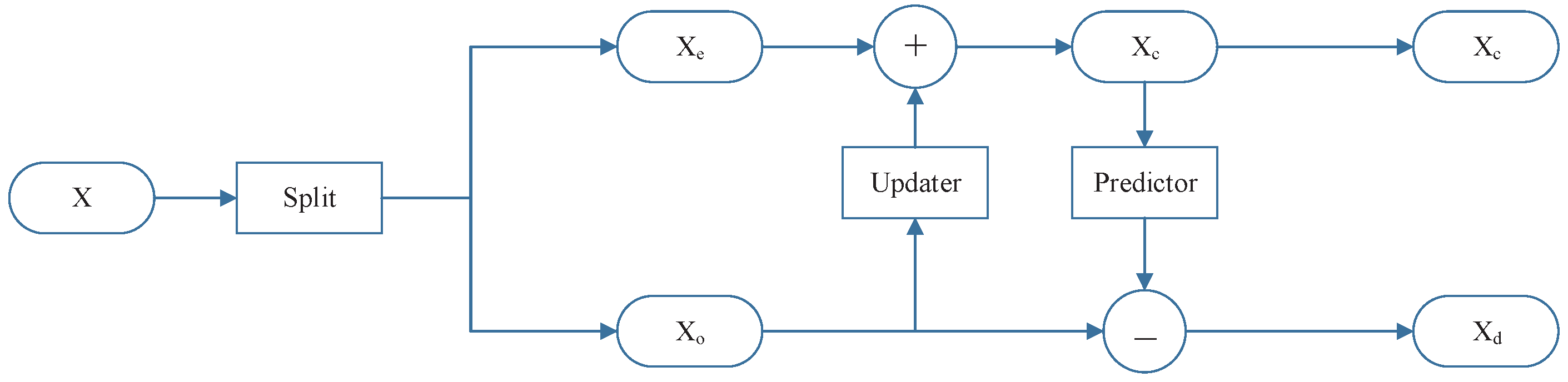
3. Adaptive Multi-Scale Wavelet Neural Network (AMSW-NN)

In this section, the proposed AMSW-NN is introduced. Compared with the BP network in the adaptive lifting scheme for one-dimensional signal, the updater and predictor in the AMSW-NN are based on a multi-scale CNN and a depthwise CNN [20]. The flowchart of the AMSW-NN is presented in Figure 2. From Figure 2, AMSW-NN consists of a frequency decomposition network (FD-Network) and a classification network (C-Network). FD-Network contains an updater, a predictor, and a selector which would be detailed introduced in the following. C-Network could be a CNN such as FCN and ResNet.

3.1. Updater

For the adaptive lifting scheme, X e [ n ] is updated by a fixed order polynomial. A predefined neighborhood is not always an optimal solution due to the noise and data distribution. To better obtain the low frequency component X c [ n ] , a multi-scale neighborhood is considered in the AMSW-NN. The structure of the updater is presented in Figure 3. Similar to [16], reflection padding is first applied to the X o [ n ] instead of the zero padding. Then, an Inception-like module is proposed to update the X e [ n ] in the multiple scales. It consists of the 1 1 , 3 1 and 5 1 convolution kernels followed by the Rectified Linear Unit (ReLU) activation and the 1 1 depthwise convolution (DWConv) kernels followed by the hyperbolic tangent (Tanh) activation. X c [ n ] could be obtained from the output of updater and X e [ n ] as Equation (2).
The rationale behind this design is that each branch of the updater models the relationship between X e [ n ] and X o [ n ] with polynomials of different orders. The different convolution kernels in each branch model this relationship with polynomials of different coefficients. DWConv guarantees the channel-dependent update without coupling. Meanwhile, DWConv could effectively reduce the number of parameters.

3.2. Predictor

When the X c [ n ] is updated, the predictor is applied to obtain the X d [ n ] . The structure of the predictor is presented in Figure 4. It contains the reflection padding with 1 1 , 3 1 and 5 1 DWConv kernels followed by the ReLU activation and the 1 1 DWConv kernels followed by the Tanh activation. X d [ n ] could be predicted by the output of predictor and X c [ n ] as Equation (3). DWConv is also used to guarantee the channel-dependent prediction.

3.3. Selector

The frequency decomposition of the time series is determined after the update and prediction in the original lifting scheme. However, the Inception-like module used in the updater and predictor results in a multi-channel feature map as Figure 2. Each channel of the feature map could be considered as a candidate frequency decomposition of the time series. The function of the selector is to choose the optimal frequency decomposition from the candidates. The structure of the selector is presented in Figure 5. A squeeze-and-excitation module [21] is applied to put the channel attention on each channel and select the optimal channel from the candidates. Given the candidate frequency decompositions D 1 , D 2 , , D M , a global average pooling (GAP) layer combined with a two-layer Multilayer Perceptron (MLP) as Equation (7) is used to learn the importance of each candidate frequency decomposition.
s i = σ ( W 2 δ ( W 1 D i ) ) ,
where W 1 R M r × M and W 2 R M × M r are the weights of the two-layer MLP. σ ( ) and δ ( ) are the ReLU and sigmoid function, respectively.

3.4. Loss Function

The loss function used to train the AMSW-NN is shown in Equation (8) which is similar to [16]. It includes a cross-entropy loss, a detail loss and a mean loss. Detail loss prefers low-magnitude detailed coefficients and mean loss promotes the X c [ n ] to maintain coarse coefficients,
l o s s = i = 1 K y i l o g ( p i ) + λ 1 H ( D ) + λ 2 ( m X c m X ) 2 ,
where K is the number of categories, H ( ) is the Huber norm. λ 1 and λ 2 are the hyperparameters.

4. Experiment

In this section, extensive experiments are performed to validate the effectiveness of the AMSW-NN. This section is divided into four parts including experimental settings, experimental results, ablation studies and complexity analysis.

4.1. Experimental Settings

In this section, the dataset used to evaluate the performance is first introduced. Then, the compared method and evaluation metric are presented. Finally, the parameter settings are provided.

4.1.1. Dataset

One of the most famous datasets for time series classification is the UCR archive. UCR archive is first introduced in 2002 [5] and updated many times. It contains time series data from different applications such as ECG and HAR. In this paper, the UCR archive including 85 datasets is used which is consistent with many published papers.

4.1.2. Compared Methods

As the discussion in Section 2, consists of a FD-Network and a C-Network. The structure of the C-Network could be designed according to the application. In this experiment, FCN, ResNet, and Inception are chosen because FCN, ResNet [11] and Inception [12] are the strong baselines and the superior methods on the UCR archive, respectively. The advantage of AMSW-NN is data-adaptive frequency decomposition. To demonstrate the performance of the FD-Network, FD-Network is replaced by a Daubechies-4 (db4) decomposition as [6] to build the compared methods.

4.1.3. Evaluation Metrics

The evaluation metrics used in this experiments include Number of Win, Average Arithmetic Ranking (AVG-AR), Average Geometric Ranking (AVG-GR) and Mean Per-Class Error (MPCE). The definitions of AVG-AR, AVG-GR, and MPCE are presented in Equations (9)–(11):
A V G A R i = 1 K r k ,
A V G G R i = r k K ,
P C E k = e k c k , M P C E i = 1 K P C E k ,
where k is the index of different datasets and i is the index of different methods, K is the number of datasets, r k , c k , and e k are the rank, the number of categories, and error rates for the k th dataset, respectively.
The critical difference defined by Equation (12) is also tested to statistically compare different methods over multiple datasets [22].
C r i t i c a l D i f f e r e n c e = q α N c ( N c + 1 ) 6 K
where critical value q α is the studentized range statistic divided by 2 , N c is the number of methods. α is set to 0.05 in the experiments.

4.1.4. Parameter Settings

AMSW-NN consists of FD-Network and C-Network. The parameter settings for FD-Network and training are listed in Table 1 and the parameter settings of C-Network is the same as [11,12]. The number of the channel used for each branch in the updater and predictor is 32, Hence, the number of the candidate frequency decomposition is 96. The ratio r in the selector is 8. AMSW-FCN is trained for 2000 epochs, and AMSW-ResNet and AMSW-Inception are trained for 1500 epochs. The Adam optimizer is employed to train the AMSW-NN with an initial learning rate l r = 0.001 , β 1 = 0.9 , β 2 = 0.999 , and ϵ = 1 × 10 8 . λ 1 and λ 2 in the loss function is set to 0.01 and 0, respectively. The model with minimum training loss is used to evaluate the performance on each dataset.

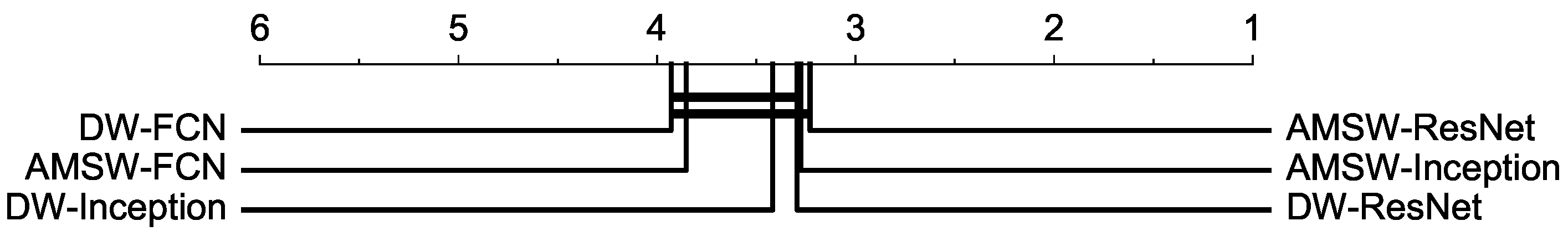
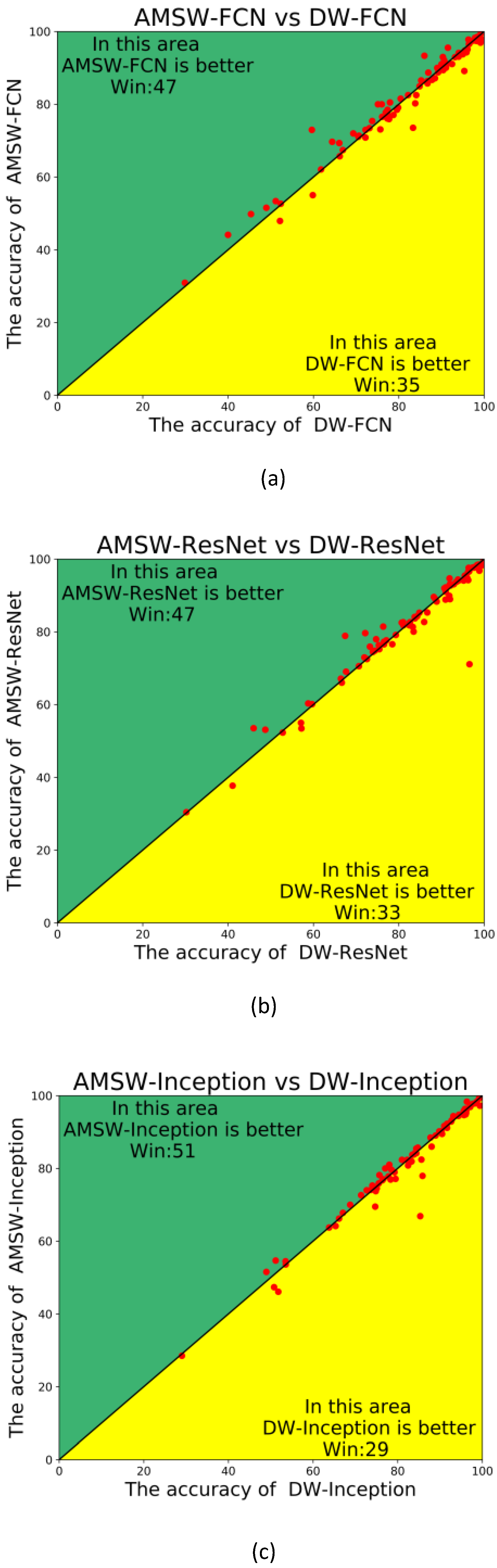
4.2. Experimental Results

In this section, the performance of the AMSW-NN on the UCR archive is reported. The accuracy rates and evaluation metrics of the AMSW-NN and compared method are shown in Table 2. DW-FCN, DW-ResNet, and DW-Inception are the abbreviations of db4 decomposition with FCN, ResNet, and Inception, respectively. To mitigate the influence of the random initialization, the evaluation is performed five times on each dataset and the average is reported to compare different methods. From Table 2, AMSW-Inception achieves the highest performance on 25 datasets and the lowest AVG-GR. AMSW-ResNet achieves the lowest AVG-AR and the second best MPCE which is just a little difference between the ResNet. Figure 6 shows the critical difference comparison of DW-FCN, DW-ResNet, DW-Inception, FCN used for the C-Network in AMSW-NN(AMSW-FCN), ResNet used for the C-Network in AMSW-NN(AMSW-ResNet), and Inception used for the C-Network in AMSW-NN(AMSW-Inception) on the UCR archive. AMSW-ResNet obtains the smallest rank compared to the other methods. Moreover, a pairwise comparison is presented in Figure 7. Compared with the DW-FCN, AMSW-FCN is better on 47 datasets and worse on 35 datasets. AMSW-ResNet is better on 47 datasets and worse on 33 datasets than DW-ResNet. AMSW-Inception is much better than DW-Inception which wins on 51 datasets and loses on 29 datasets. It proves that no matter what C-Network is selected, FD-Network obtains a better frequency decomposition than db4 decomposition.
Furthermore, it could be observed that no model could achieve the best performance on all datasets from the results listed in Table 2. However, an empirical guidance could be summarized. AMSW-Inception adopts the Inception architecture to discover the patterns in the different scales. Hence, AMSW-Inception obtains the highest accuracy on the datasets such as “CricketX” and “UWaveGestureLibraryX” which have the large intra-class difference because a single-scale convolution is insufficient to extract the discriminative pattern on these datasets. In contrast, AMSW-FCN and AMSW-ResNet are more suitable for the datasets such as “Beef” and “Meat”which have the small intra-class difference.

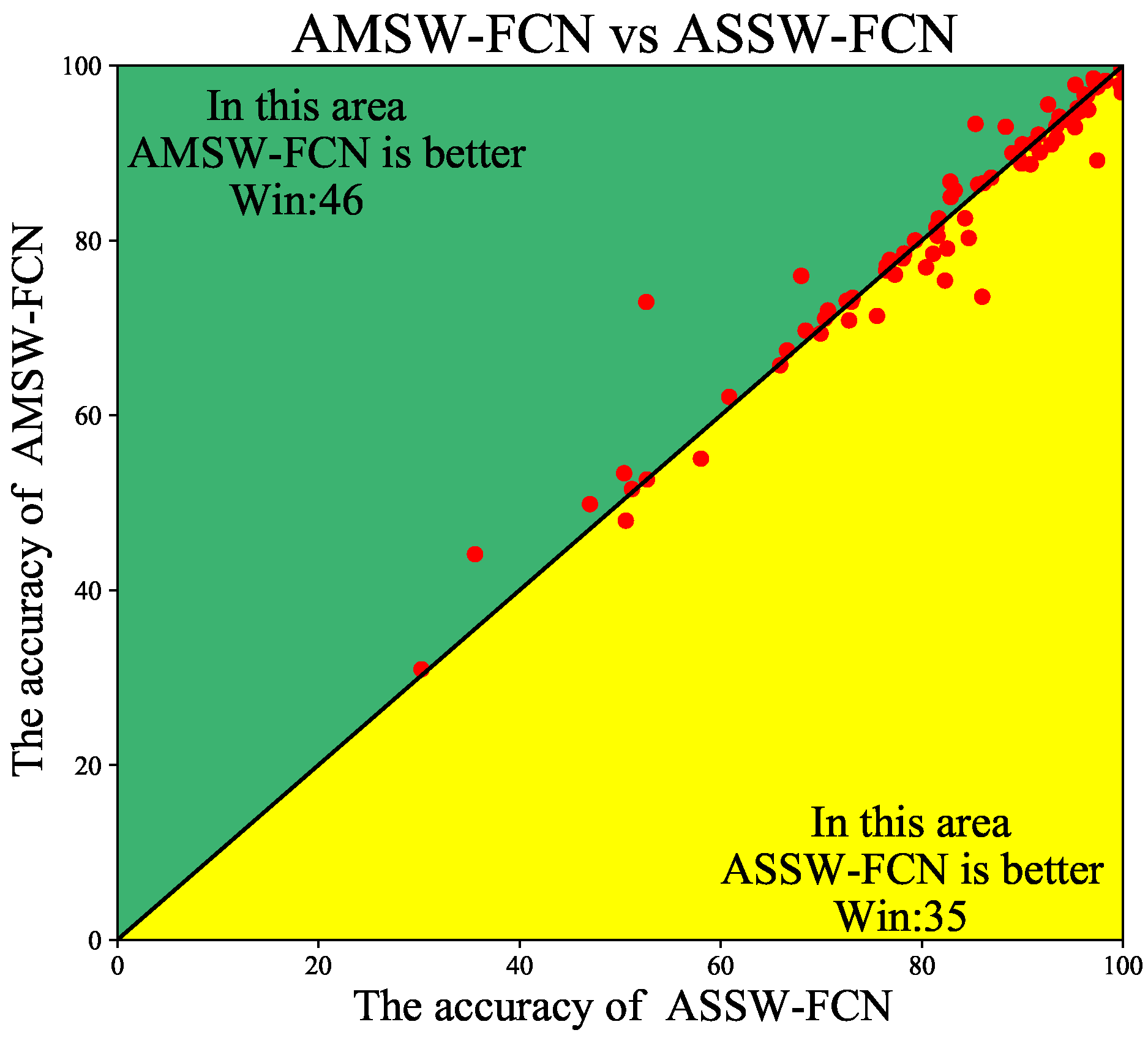
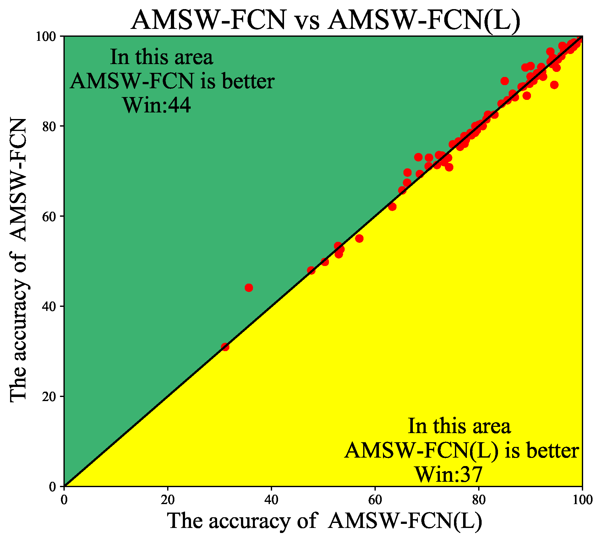
4.3. Ablation Studies

In this section, the effectiveness of the multi-scale structure and hyperparameters of loss function are analyzed. To validate the superiority of the multi-scale updater and predictor for AMSW-NN, a single-scale version of AMSW-FCN called ASSW-FCN is designed. Compared to the AMSW-FCN, ASSW-FCN only applies the 1 3 convolution kernel size to update and predict. The pairwise comparison between AMSW-FCN and ASSW-FCN is shown in Figure 8. Compared to the ASSW-FCN, AMSW-FCN achieves a better performance on the UCR archive which proves the effectiveness of the multi-scale structure.
The loss function for training the AMSW-NN contains the detail loss and mean loss as presented in Equation (8). In Section 4.1, λ 2 is set to 0 which means the high frequency is not suppressed. In this section, λ 2 is set to 0.01 as [16] to suppress the detailed coefficients. AMSW-FCN with this loss function called AMSW-FCN(L) is trained on the UCR archive again. The pairwise comparison between AMSW-FCN and AMSW-FCN(L) is shown in Figure 9.
As shown in Figure 9, the performance of AMSW-FCN is slightly better than AMSW-FCN(L). The reasonable explanation is that AMSW-FCN suppresses the high frequency and AMSW-FCN(L) does not. If the high frequency is noise rather than detail, it is expected that AMSW-FCN is better than AMSW-FCN(L), and vice versa. For instance, AMSW-FCN achieves the higher accuracy on the “CricketX”, “CricketY” and “CricketZ”. Figure 10 presents some training samples from the “CricketX”, “CricketY” and “CricketZ”. It indicates that high frequency noise exists.

4.4. Complexity Analysis

AMSW-NN is composed of the FD-Network and C-Network. Compared with the DW-NN, the extra computational complexity is from the FD-Network. It is proportional to the number of the convolution kernel of the updater and predictor. Moreover, it is also proportional to the ratio r for the selector. Compared with the C-Network, the parameter learnt in the FD-Network is relatively small because the DWConv is used. The number of the learnable parameters for FD-Network and different classification networks is shown in Table 3.

5. Conclusions

In this paper, an adaptive multi-scale wavelet neural network called AMSW-NN for Time Series Classification is proposed. Compared with the frequency decomposition by the predefined wavelet basis, AMSW-NN adopts the multi-scale and depthwise convolution with the squeeze-and-excitation module to build the learnable updater, predictor and selector to adaptively separate the low frequency component and high frequency component from the time series which has a better generalization performance. Extensive experiments on the UCR archive show that the AMSW-NN indeed achieves a better performance than the classical wavelet decomposition combined with the neural network. In future work, we will attempt to extend the AMSW-NN to more complex applications. First, we want to modify the AMSW-NN to classify multivariate time series. Furthermore, second, we hope to find an adaptive strategy to better split the time series before the update.

Author Contributions

Methodology, K.O.; supervision, Y.H. and S.Z.; writing—original draft, K.O.; writing—review and editing, Y.H. and Y.Z. All authors have read and agreed to the published version of the manuscript.

Funding

This work was funded by the National Natural Science Foundation of China under Grant No.61903373.

Institutional Review Board Statement

Not applicable.

Informed Consent Statement

Not applicable.

Data Availability Statement

The data used in this study is from the UCR archive which can be found here: http://www.timeseriesclassification.com/, accessed on 16 June 2021.

Conflicts of Interest

The authors declare no conflict of interest.

References

  1. Liu, C.L.; Hsaio, W.H.; Tu, Y.C. Time series classification with multivariate convolutional neural network. IEEE Trans. Ind. Electron. 2018, 66, 4788–4797. [Google Scholar] [CrossRef]
  2. Ordóñez, F.J.; Roggen, D. Deep convolutional and lstm recurrent neural networks for multimodal wearable activity recognition. Sensors 2016, 16, 115. [Google Scholar] [CrossRef] [PubMed] [Green Version]
  3. Übeyli, E.D. Wavelet/mixture of experts network structure for EEG signals classification. Expert Syst. Appl. 2008, 34, 1954–1962. [Google Scholar] [CrossRef]
  4. Al-Jowder, O.; Kemsley, E.; Wilson, R.H. Detection of adulteration in cooked meat products by mid-infrared spectroscopy. J. Agric. Food Chem. 2002, 50, 1325–1329. [Google Scholar] [CrossRef] [PubMed]
  5. Dau, H.A.; Bagnall, A.; Kamgar, K.; Yeh, C.C.M.; Zhu, Y.; Gharghabi, S.; Ratanamahatana, C.A.; Keogh, E. The UCR time series archive. IEEE/CAA J. Autom. Sin. 2019, 6, 1293–1305. [Google Scholar] [CrossRef]
  6. Wang, J.; Wang, Z.; Li, J.; Wu, J. Multilevel wavelet decomposition network for interpretable time series analysis. In Proceedings of the 24th ACM SIGKDD International Conference on Knowledge Discovery & Data Mining, London, UK, 19–23 August 2018; pp. 2437–2446. [Google Scholar]
  7. Ye, L.; Keogh, E. Time series shapelets: A new primitive for data mining. In Proceedings of the 15th ACM SIGKDD International Conference on Knowledge Discovery and Data Mining, Paris, France, 28 June–12 July 2009; pp. 947–956. [Google Scholar]
  8. Lines, J.; Bagnall, A. Time series classification with ensembles of elastic distance measures. Data Min. Knowl. Discov. 2015, 29, 565–592. [Google Scholar] [CrossRef]
  9. Schäfer, P. The BOSS is concerned with time series classification in the presence of noise. Data Min. Knowl. Discov. 2015, 29, 1505–1530. [Google Scholar] [CrossRef]
  10. Schäfer, P.; Leser, U. Fast and accurate time series classification with weasel. In Proceedings of the 2017 ACM on Conference on Information and Knowledge Management, Singapore, 6–10 November 2017; pp. 637–646. [Google Scholar]
  11. Wang, Z.; Yan, W.; Oates, T. Time series classification from scratch with deep neural networks: A strong baseline. In Proceedings of the 2017 International Joint Conference on Neural Networks (IJCNN), Anchorage, AK, USA, 14–19 May 2017; pp. 1578–1585. [Google Scholar]
  12. Fawaz, H.I.; Lucas, B.; Forestier, G.; Pelletier, C.; Schmidt, D.F.; Weber, J.; Webb, G.I.; Idoumghar, L.; Muller, P.A.; Petitjean, F. Inceptiontime: Finding alexnet for time series classification. Data Min. Knowl. Discov. 2020, 34, 1936–1962. [Google Scholar] [CrossRef]
  13. Li, D.; Bissyandé, T.F.; Klein, J.; Traon, Y.L. Time series classification with discrete wavelet transformed data. Int. J. Softw. Eng. Knowl. Eng. 2016, 26, 1361–1377. [Google Scholar] [CrossRef] [Green Version]
  14. Akansu, A.N.; Haddad, P.A.; Haddad, R.A.; Haddad, P.R. Multiresolution Signal Decomposition: Transforms, Subbands, and Wavelets; Academic Press: Cambridge, MA, USA, 2001. [Google Scholar]
  15. Sweldens, W. The lifting scheme: A construction of second generation wavelets. SIAM J. Math. Anal. 1998, 29, 511–546. [Google Scholar] [CrossRef] [Green Version]
  16. Rodriguez, M.X.B.; Gruson, A.; Polania, L.; Fujieda, S.; Prieto, F.; Takayama, K.; Hachisuka, T. Deep adaptive wavelet network. In Proceedings of the IEEE/CVF Winter Conference on Applications of Computer Vision, Waikola, HI, USA, 5–9 January 2021; pp. 3111–3119. [Google Scholar]
  17. Sweldens, W. Wavelets and the lifting scheme: A 5 minute tour. Zamm-Z. Angew. Math. Mech. 1996, 76, 41–44. [Google Scholar]
  18. Ma, H.; Liu, D.; Xiong, R.; Wu, F. iWave: CNN-Based Wavelet-Like Transform for Image Compression. IEEE Trans. Multimed. 2019, 22, 1667–1679. [Google Scholar] [CrossRef]
  19. Zheng, Y.; Wang, R.; Li, J. Nonlinear wavelets and BP neural networks adaptive lifting scheme. In Proceedings of the 2010 International Conference on Apperceiving Computing and Intelligence Analysis Proceeding, Chengdu, China, 17–19 December 2010; pp. 316–319. [Google Scholar]
  20. Chollet, F. Xception: Deep learning with depthwise separable convolutions. In Proceedings of the IEEE Conference on Computer Vision and Pattern Recognition, Honolulu, HI, USA, 21–26 July 2017; pp. 1251–1258. [Google Scholar]
  21. Hu, J.; Shen, L.; Sun, G. Squeeze-and-excitation networks. In Proceedings of the IEEE Conference on Computer Vision and Pattern Recognition, Salt Lake City, UT, USA, 18–23 June 2018; pp. 7132–7141. [Google Scholar]
  22. Demšar, J. Statistical comparisons of classifiers over multiple data sets. J. Mach. Learn. Res. 2006, 7, 1–30. [Google Scholar]
Figure 1. The flowchart of the lifting scheme.
Information 12 00252 g001
Figure 2. The flowchart of the AMSW-NN.
Information 12 00252 g002
Figure 3. The structure of the updater. Padding in the updater denotes the reflection padding.
Information 12 00252 g003
Figure 4. The structure of the predictor. Padding in the predictor denotes the reflection padding.
Information 12 00252 g004
Figure 5. The structure of the selector.
Information 12 00252 g005
Figure 6. Critical difference diagram showing statisitical difference comparison of DW-FCN, DW-ResNet, DW-Inception, AMSW-FCN, AMSW-ResNet, and AMSW-Inception on the UCR archive.
Information 12 00252 g006
Figure 7. The results of the pairwise comparison. (a) shows the accuracy of AMSW-FCN against DW-FCN, (b) shows the accuracy of AMSW-ResNet against DW-ResNet, (c) shows the accuracy of AMSW-Inception against DW-Inception.
Information 12 00252 g007
Figure 8. The pairwise comparison between AMSW-FCN and ASSW-FCN.
Information 12 00252 g008
Figure 9. The pairwise comparison between AMSW-FCN and AMSW-FCN(L).
Information 12 00252 g009
Figure 10. The training samples from the “CricketX”, “CricketY” and “CricketZ”. The samples from the same class are listed in the same row. High frequency noise could be observed in the red circle.
Information 12 00252 g010
Table 1. Parameter settings for FD-Network and training.
ParameterValue
Kernel size5, 3, 1
FD channel32
Ratio8
Training epoch1500/2000
Learning rate0.001
λ 1 0.01
λ 2 0
Table 2. Accuracy rates and evaluation metrics of the DW-FCN (DWF), DW-ResNet (DWR), DW-Inception (DWI), AMSW-FCN (AMSWF), AMSW-ResNet (AMSWR), and AMSW-Inception (AMSWI) on the UCR archive. The accuracy rate listed in this Table for each dataset is the average of five evaluations on the testing set. For each evaluation, the model corresponding to the minimum training loss is used to predict the label and calculate the accuracy on the testing set. The accuracy rates keep three decimal places for clariy. The highest value (bold) in each dataset is actually based on the original results.
DatasetDWFAMSWFDWRAMSWRDWIAMSWI
Adiac0.8490.8500.8380.8370.7650.770
ArrowHead0.8670.8640.8480.8530.8340.838
Beef0.7600.8000.7470.7800.7130.727
BeetleFly0.8900.9000.9100.9100.7800.810
BirdChicken0.9000.9100.9200.8900.8800.860
Car0.9030.9300.9070.9200.9100.917
CBF0.9820.9740.9890.9680.9960.997
ChlorineConcentration0.7960.7850.8350.8010.8560.824
CinCECGTorso0.8520.8660.8370.8410.8440.855
Coffee1.0001.0001.0001.0001.0001.000
Computers0.7740.7850.7640.7680.7480.738
CricketX0.7740.7690.8110.8180.8380.838
CricketY0.7730.7790.8100.8270.8410.843
CricketZ0.7980.7910.8430.8430.8450.855
DiatomSizeReduction0.9070.9170.9390.9410.9310.944
DistalPhalanxOutlineAgeGroup0.7060.7140.7250.7250.7470.695
DistalPhalanxOutlineCorrect0.7730.7610.7850.7660.7780.778
DistalPhalanxTW0.6600.6940.6760.6910.6530.642
Earthquakes0.7570.7310.7440.7480.7370.741
ECG2000.9040.8940.8820.8960.8980.902
ECG50000.9400.9410.9340.9370.9440.944
ECGFiveDays0.9960.9781.0001.0000.9990.999
ElectricDevices0.6620.6570.6660.6600.6610.662
FaceAll0.8780.8670.8250.8180.8240.808
FaceFour0.9320.9300.9550.9550.9270.932
FacesUCR0.9540.9480.9620.9640.9560.956
FiftyWords0.7050.7110.7650.7660.8310.818
Fish0.9810.9760.9870.9850.9860.983
FordA0.9400.9310.9610.9480.9570.958
FordB0.8220.8250.8260.8260.8480.857
GunPoint0.9961.0001.0000.9990.9920.992
Ham0.7220.7090.7540.7520.6700.678
HandOutlines0.8690.8870.9290.9310.9590.964
Haptics0.5230.5270.5710.5500.5350.545
Herring0.6440.6970.5880.6030.6880.700
InlineSkate0.4000.4410.4110.3770.5180.461
InsectWingbeatSound0.4530.4980.5970.6020.6380.638
ItalyPowerDemand0.9590.9490.9600.9440.9600.948
LargeKitchenAppliances0.9100.9010.9090.8890.8900.891
Lightning20.7380.7540.7210.7970.7700.800
Lightning70.8380.8030.8330.8140.8330.819
Mallat0.9640.9650.9650.9660.9590.959
Meat0.8600.9330.9770.9770.9570.947
MedicalImages0.7610.7660.7650.7730.7830.769
MiddlePhalanxOutlineAgeGroup0.4900.5160.4600.5350.4900.516
MiddlePhalanxOutlineCorrect0.7510.8000.7640.8140.7920.790
MiddlePhalanxTW0.5120.5340.4870.5310.5120.547
MoteStrain0.9060.9210.9100.9220.8770.885
NonInvasiveFetalECGThorax10.9610.9510.9520.9410.9620.958
NonInvasiveFetalECGThorax20.9580.9430.9570.9500.9580.958
OliveOil0.6930.7200.8670.8530.7270.740
OSULeaf0.9790.9830.9640.9760.9260.929
PhalangesOutlinesCorrect0.8040.8150.8070.8250.8100.824
Phoneme0.2990.3090.3020.3040.2900.285
Plane1.0001.0001.0001.0001.0001.000
ProximalPhalanxOutlineAgeGroup0.8410.8250.8600.8270.8440.842
ProximalPhalanxOutlineCorrect0.8920.8880.9180.8990.9030.902
ProximalPhalanxTW0.7870.7710.7710.7770.7550.759
RefrigerationDevices0.5220.4790.5280.5230.5080.474
ScreenType0.5980.5500.5720.5340.5350.536
ShapeletSim0.8330.7360.9660.7110.8530.669
ShapesAll0.9120.9100.9200.9310.9160.923
SmallKitchenAppliances0.7770.7590.7320.7590.7570.782
SonyAIBORobotSurface10.9530.8920.9630.9420.8590.780
SonyAIBORobotSurface20.9500.9380.9190.9470.9050.895
StarLightCurves0.9750.9750.9730.9770.9780.978
Strawberry0.9820.9820.9840.9840.9820.979
SwedishLeaf0.9650.9670.9580.9520.9620.952
Symbols0.9830.9850.9790.9790.9710.969
SyntheticControl0.9910.9690.9930.9820.9940.973
ToeSegmentation10.9630.9780.9390.9440.9560.959
ToeSegmentation20.9250.9110.9220.9280.9450.948
Trace1.0001.0001.0001.0001.0001.000
TwoLeadECG0.9920.9950.9990.9980.9630.983
TwoPatterns0.9150.9561.0001.0001.0001.000
UWaveGestureLibraryAll0.8670.8570.8850.8910.9630.964
UWaveGestureLibraryX0.7690.7780.7930.7910.8220.824
UWaveGestureLibraryY0.6690.6740.7070.7060.7640.767
UWaveGestureLibraryZ0.7310.7340.7390.7450.7660.771
Wafer0.9980.9980.9990.9980.9970.997
Wine0.5960.7300.6740.7890.7850.796
WordSynonyms0.6180.6210.6640.6710.7400.753
Worms0.7790.8050.7530.7640.7950.771
WormsTwoClass0.7220.7300.7190.7300.7510.745
Yoga0.8850.8720.8890.8830.9170.912
Number of win131623161625
AVG-AR3.8243.7293.1533.0823.2713.141
AVG-GR3.2973.1382.6122.6582.7652.536
MPCE0.0470.0460.0440.0440.0450.046
Table 3. The number of the learnable parameters for AMSW-NN.
ComponentParameter Amount
FD-Network3564
FCN271,154
ResNet526,964
Inception426,642
Publisher’s Note: MDPI stays neutral with regard to jurisdictional claims in published maps and institutional affiliations.

